Abstract
The Global Navigation Satellite System Interferometric Reflectometry (GNSS-IR) has demonstrated significant potential for soil moisture content (SMC) monitoring due to its high spatiotemporal resolution. However, GNSS-IR inversion experiments are notably influenced by vegetation and meteorological factors. To address these challenges, this study proposes a multi-factor SMC inversion method. Six GNSS stations from the Plate Boundary Observatory (PBO) were selected as study sites. A low-order polynomial was applied to separate the reflected signals, extracting parameters such as phase, frequency, amplitude, and effective reflector height. Auxiliary variables, including the Normalized Microwave Reflection Index (NMRI), cumulative rainfall, and daily average evaporation, were used to further improve inversion accuracy. A multi-factor SMC inversion dataset was constructed, and three machine learning models were selected to develop the SMC prediction model: Support Vector Regression (SVR), suitable for small and medium-sized regression tasks; Convolutional Neural Networks (CNN), with robust feature extraction capabilities; and NRBO-XGBoost, which supports automatic optimization. The multi-factor SMC inversion method achieved remarkable results. For instance, at the P038 station, the model attained an R2 of 0.98, with an RMSE of 0.0074 and an MAE of 0.0038. Experimental results indicate that the multi-factor inversion model significantly outperformed the traditional univariate model, whose R2 (RMSE, MAE) was only 0.88 (0.0179, 0.0136). Further analysis revealed that NRBO-XGBoost surpassed the other models, with its average R2 outperforming SVR by 0.11 and CNN by 0.03. Additionally, the analysis of different surface types showed that the method achieved higher accuracy in grassland and open shrubland areas, with all models reaching R2 values above 0.9. Therefore, the accuracy of the multi-factor SMC inversion model was validated, supporting the practical application of GNSS-IR technology in SMC inversion.
1. Introduction
Soil moisture content (SMC) is an important component of the water cycle, and high spatiotemporal resolution SMC monitoring is crucial for agricultural production, ecological conservation, and meteorological research [1,2,3,4]. Currently, SMC monitoring primarily relies on field observations, satellite remote sensing, and data assimilation [5,6,7]. Field measurement methods, such as the oven-drying method, Time Domain Reflectometry [8], and Frequency Domain Reflectometry [9], can provide high-precision data. However, due to spatiotemporal and geographical constraints, it is difficult to achieve large-scale, long-term monitoring [10]. Satellite remote sensing technologies, including active/passive microwave remote sensing [11,12], optical remote sensing [13], and multi-source remote sensing [14], offer significant advantages for large-scale SMC monitoring. However, they struggle to meet accuracy requirements in small-scale studies, such as in the construction of small watershed hydrological models, precision agriculture, and environmental monitoring. Although model simulations and data assimilation can improve prediction accuracy, they are limited by the accuracy of the input data [15]. GNSS-IR has been widely used to invert surface environmental parameters owing to its advantages, including low cost, high spatiotemporal resolution, and strong cloud penetration capabilities [16,17,18].
Numerous researchers have made significant advancements in GNSS-IR-based SMC inversion in recent years [19]. Larson et al. introduced a linear model for SMC inversion by separating the phase of GPS L2 band reflected signals [20]. Pierdicca validated the feasibility of GNSS-IR-based SMC inversion by developing a theoretical model, with simulation results showing trends consistent with experimental data [21]. Chew et al. carried out a comprehensive analysis on the relationship between SMC and phase, amplitude, and frequency, finding that phase has the highest correlation with SMC [22]. Tabibi inverted SMC using the L5 band, and the inversion results were more consistent with those of the L2 band [23]. Researchers have proposed various improvement methods to enhance the accuracy of SMC inversion. Han proposed a semi-empirical signal-to-noise ratio (SNR) model, which further improved the inversion accuracy [24]. Liang improved the issue of sudden jumps in single-satellite inversion by using a sliding window-based selection mechanism [25]. Jin obtained better inversion results by integrating dual-frequency phase observations using the entropy method [26]. Additionally, the introduction of the amplitude attenuation factor (AAF) significantly improved the accuracy of SMC inversion [27]. Meanwhile, Zhu’s experiment demonstrated that better results can be obtained in SMC inversion with satellite elevation angles ranging from 5° to 30° and arc lengths exceeding 20° [28].
Currently, most GNSS research is conducted under bare-soil conditions, but in practical applications, it is inevitably affected by vegetation effects. Lv proposed using multivariate adaptive regression splines (MARS) to mitigate the impact of vegetation during SMC inversion, and the model achieved promising results [29]. Using empirical mode decomposition significantly enhances the precision of SMC inversion [30]. In addition, the integration of triple-frequency signals can also enhance inversion accuracy [31]. The NMRI derived from multipath data can effectively minimize the influence of vegetation water content [32,33]. However, traditional linear models struggle to account for the interactive effects of multiple surface factors, whereas machine learning algorithms construct input-output mappings through training data, effectively capturing nonlinear and latent relationships. Pan et al. successfully inverted vegetation water content by integrating GNSS-IR and MODIS data [34]. Ding inverted SMC using a backpropagation neural network, Gaussian process regression, and random forest models, with the random forest achieving the highest accuracy [35]. Zhang utilized an integrated machine learning approach with satellite-based GNSS-R and multisource remote sensing data to invert vegetation water content [36]. Li significantly improved the correlation between feature parameters and SMC using the improved HVCE fusion method [37]. Huang employed the machine learning model SSA-ELM to invert SMC, achieving greater model accuracy compared to the BP neural network [38].
In the aforementioned studies, the inversion of SMC typically relied on a single SNR feature parameter, leading to insufficient model robustness and a tendency toward overfitting. While existing methods focus on reducing vegetation interference, they fail to adequately address the potential impact of climate, surface characteristics, and other environmental factors on inversion results. Some studies directly input real-time rainfall data into models, overlooking the delayed cumulative effects of precipitation. Although Xian et al. eliminated temporal interference by developing a cumulative precipitation correction strategy, they did not consider other influencing factors [39]. Therefore, to achieve more accurate SMC inversion, it is essential to consider multiple environmental factors from various sources and mitigate their interference with inversion results.
In this study, plots with different vegetation coverage types were studied. By extracting GPS satellite observation data, including phase, frequency, amplitude, NMRI, and Heff, and incorporating environmental factors such as cumulative precipitation and evaporation, a multi-factor inversion dataset was constructed. Subsequently, SVR, CNN, and NRBO-XGBoost models were employed to develop the SMC inversion model. The research objectives include: (1) comparing and analyzing the correlation between NMRI and vegetation water content; (2) evaluating the performance of traditional single-factor SMC inversion models versus multi-factor SMC inversion models; (3) assessing the effectiveness of the multi-factor SMC inversion model under different vegetation cover conditions; and (4) analyzing the performance of SVR, CNN, and NRBO-XGBoost in multi-factor SMC inversion.
2. Materials and Methods
2.1. Methodology
The GNSS satellite signal reflects off environmental surfaces such as the ground, buildings, and vegetation during the propagation process, forming a reflection signal (Ar). The direct (Ad) and reflected (Ar) signals combine at the GNSS antenna junction to form a relatively stable interference signal (Figure 1) [20]. The ground-based GNSS receiver captures the interference signal, which is recorded as the SNR.
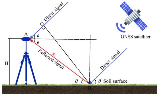
Figure 1.
GNSS-IR SMC inversion schematic diagram. The blue lines represent direct signals, while the red line indicates reflected signal.
The reflection characteristics of the object’s surface determine the interference phenomenon. The phase and frequency changes of the reflected signal are strongly linked to the physical properties of the surface, including its dielectric constant and roughness. Therefore, by analyzing the characteristics of the interference signal, the properties of the surface can be deduced. The mathematical model for the SNR recorded by the receiver is given by [20,40]:
In the equation, Ad and Ar represent the amplitudes of the direct and reflected signals, respectively, φ is the delay phase, in view of the numerical difference between the multipath straight and reflection components, Ad ≥ Ar. In addition, with the variation in the GNSS satellite’s elevation angle, changes to Ad, Ar and φ, lead to fluctuations in the SNR, with the overall trend of the SNR following a parabolic curve. By removing the amplitude components from the direct signal and a few multipath reflections, the remaining reflection components can be approximately represented using a cosine function model [35]:
In the equation, SNRr represents the residual sequence at low elevation angles containing reflection information, Ar represents the reflected signal’s amplitude, H is the antenna height, θ represents the satellite elevation angle, λ represents the wavelength, and φ denotes the delay phase. Suppose , , then Equation (2) can be expressed as [33]:
By performing LSP spectral analysis on the reflected signal, the frequency f is obtained. Subsequently, Ar and φ can be obtained through fitting. Studies have shown that the frequency, amplitude, and phase of the satellite reflected signal exhibit a strong correlation with the SMC, which can be utilized for its inversion [20,41].
2.2. Sites and Data
2.2.1. Study Area
This study utilizes data from six Plate Boundary Observatory (PBO) stations across the U.S.: P038, P389, P309, P472, P742, and Bkap (https://data.unavco.org/archive/gnss/rinex/, accessed on 14 April 2024). The selected stations are located in the western United States (Figure 2), covering a range of climate zones, including semi-arid (P038, New Mexico), temperate continental (P389, Oregon), Mediterranean (P309, P472, P742, California), and desert (Bkap, Mojave Desert). During the observation period, the total accumulated rainfall at P038 reached 200 mm, with a single-day peak of 39.1 mm, while the maximum single-event rainfall at P472 did not exceed 5 mm (Figure 3). The vegetation types at each site are shown in Table 1. The receivers used in the experiment are capable of receiving dual-frequency GPS L1/L2 data with a sampling interval of 15 s. Based on the first Fresnel zone model, a signal reflection area was constructed (Figure 4) to quantify the impact of surface reflections on multipath effects.

Figure 2.
Study area overview map.
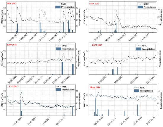
Figure 3.
SMC and rainfall variation trends. The line chart represents measured SMC, while the bar chart represents rainfall.

Table 1.
Site location and receiver related parameters.
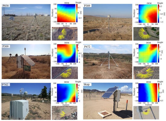
Figure 4.
Digital Elevation Model and surrounding environment of P038, P389, P309, P472, P742, and Bkap.
SMC and rainfall data are obtained from the International Soil Moisture Network, which is widely used in SMC inversion studies due to its high quality and representativeness. Evaporation data are calculated using the Hargreaves method, with relevant data also sourced from this network. The NDVI is obtained from Sentinel-2 imagery through the Google Earth Engine platform. Operated by the European Space Agency, Sentinel-2 provides a 10-m resolution, making it ideal for vegetation dynamics monitoring (Table 2).
Table 2.
Data sources.
2.2.2. Data Processing Workflow
This study processes GNSS data using the MATLAB R2022b platform, with the following technical workflow (Figure 5): (1) The observation files and broadcast ephemeris are processed using GIRAS 2021, an open-source software package. After quality control is applied to remove anomalous data, the frequency, amplitude, and phase of the reflected signal are estimated based on the satellite’s elevation angle, azimuth angle, and SNR parameters. The NMRI and Heff are then obtained from multipath observations and Lomb–Scargle spectral analysis, respectively. (2) An entropy-based fusion method is used to integrate multi-satellite observation data, and the correlation between the fused NMRI and NDVI is verified. (3) Pearson correlation analysis is performed between the feature parameters of multi-satellite reflected signals (frequency, amplitude, phase, NMRI, and Heff), key climate factors (average temperature, daily rainfall, cumulative rainfall, and evaporation), and SMC. The optimal variables are selected to construct a multi-factor dataset. (4) The dataset is separated into training and testing subsets, and the SVR, CNN, and NRBO-XGBoost inversion models are developed and evaluated for accuracy.
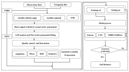
Figure 5.
Flowchart for multi-factor soil moisture content inversion.
2.3. GNSS-IR Soil Moisture Inversion Dataset
2.3.1. Extraction of Reflection Signal Feature Parameters
The trajectory of the satellite reflection point is determined by the elevation angle, azimuth angle, and antenna height, which together describe the satellite’s position relative to the receiver [42]. Therefore, the azimuth angle can be reasonably selected according to the reflection point trajectory to maintain consistency with the surrounding environment (Figure 6).
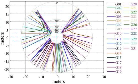
Figure 6.
P038 (DOY: 2017-120) satellite elevation angle at 5~30° reflection point trajectory.
The SNR of low-elevation satellites is significantly affected by multipath effects, exhibiting periodic oscillations. As the elevation angle increases, antenna gain improves, leading to a more stable SNR [22,43]. Figure 7a illustrates the oscillatory characteristics of the SNR at lower satellite elevation angles, while Figure 7b presents the detailed results of SNR sequence detrending. The blue line denotes the original SNR; the red line denotes the fitted direct signal; the black line indicates the reflected signal; the red rectangular box represents the oscillation characteristics of SNR when the satellite elevation angle is between 5° and 30°. The reflected signal contains the required key parameters such as phase, frequency, amplitude, and Heff. In this experiment, suitable azimuth and elevation angles (Table 3) were selected based on the vegetation coverage at each site (Figure 3).
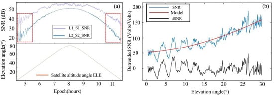
Figure 7.
(a) P038 (DOY:145 PRN: G10) SNR data for GPS satellite. The red rectangular box represents the oscillation characteristics of SNR when the satellite elevation angle is between 5° and 30°. (b) Figure (a) on the left shows the SNR data within the red rectangle, including separated reflected signals. The blue line represents the original SNR data, the black line represents the reflected signal data, and the red line represents the curve of the low-order polynomial model.
Table 3.
Satellite azimuth, elevation angle, and reflection height.
2.3.2. Normalized Microwave Reflection Index
NDVI is widely applied for retrieving VWC [44]. In a specific region, as NDVI increases, the reflection of microwave signals from the soil surface gradually weakens [32]. Therefore, NDVI can effectively reflect the extent to which vegetation affects the signal. Under different vegetation cover conditions, the NMRI, calculated from GNSS pseudorange multipath errors, fluctuates with changes in vegetation growth. The trend of NMRI variations closely aligns with that of NDVI, indicating a strong correlation between the two (Figure 8) [45]. The pseudorange multipath error of the L1 carrier (MP1) is as follows:
where, P1 represents the pseudorange observation on the L1 carrier, f represents the frequency of the band, , , and φ represents the phase of the carrier.
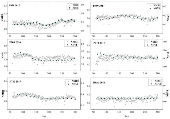
Figure 8.
Scatter plot trend between NDVI and NMRI. Gray dots represent NMRI, while dark green dots represent NDVI.
According to the epoch-changing MP1, the daily RMS of MP1 for each satellite is calculated. Subsequently, the weighted sum of the daily observations of each satellite is used to calculate the RMS of the daily MP1. NMRI is expressed as:
In the equation, RMSMP1 represents the RMS value of MP1 for a single day; max(RMSMP1) is the average value of RMSMP1, derived from the upper 5% of RMSMP1 values arranged in descending order.
2.4. Construction of the SMC Inversion Model and Evaluation of Model Accuracy
This study employs machine learning techniques to construct an SMC prediction model. It is assumed that there exists a nonlinear relationship between the SMC and multiple feature variables (x1, x2, …, xn), and the model can be expressed as follows:
In the equation, the prediction of SVR is obtained through a weighted summation calculated by kernel functions and Lagrange multipliers. Neural network predictions are derived from a series of multi-layer nonlinear mappings of weight matrices and bias terms. XGBoost predictions are obtained by combining the outputs of several decision trees, with each tree’s output corresponding to the prediction for input features x1, x2, …, xn.
2.4.1. Support Vector Regression
Support Vector Regression is built upon Support Vector Machines, designed to effectively address nonlinear regression problems by mapping data into a high-dimensional space [46,47]. Assuming the training samples (xi, yi), where i = 1, …, N, the SVR regression model is as follows:
Subject to the following constraints:
In Equation (7), ‖w‖2 represents the sum of the squares of the weight vector, which indicates the complexity of the model. and are the slack variables used to handle samples with errors greater than ε. C is the regularization parameter, used to balance the model’s complexity and training error, while ϵ is the error tolerance, controlling the model’s tolerance for errors.
For Equation (7), The original problem’s optimal solution is usually obtained by solving the Lagrange dual problem of the above model:
where K (xi + xj) is called a kernel function, satisfying the Mercer condition and The radial basis function (RBF) is a universal type of kernel.
Here, represents the kernel width coefficient, and . In this study, the regularization parameter C is set to 4.0, the error tolerance ε is 0.01, and γ is 0.8.
2.4.2. Convolutional Neural Network
Convolutional Neural Networks, common in fields like imaging and natural language processing, are characterized by local connections and weight sharing [48,49,50]. The core idea is to extract features through convolutional layers, progressively learning from the data at each layer. These features are then integrated for regression analysis. During CNN training, the weights are typically updated using the backpropagation algorithm. The convolutional layer is defined as:
In the equation, represents the input to the j convolutional kernel of the I layer, and is also the output of the I − 1 layer. denotes the activation function, and Mj denotes the set of input mapping layers. represents the convolution kernel, is called the bias term.
The fully connected layer is expressed as follows:
where XI+1(j) represents the value of the j output neuron in the I + 1 layer, and is the weight matrix of the j convolutional kernel in the i layer. In this study, the convolutional kernel size is set to 3 × 1. To extract higher-level features, the first layer consists of 16 neurons, and the second layer contains 32 neurons. The starting learning rate is 0.01, the activation function uses ReLU, and SGDM is used as the optimization strategy.
2.4.3. Newton–Raphson-Based Optimization XGBoost
- (1)
- Newton–Raphson-Based Optimizer
The NRBO generates an initial random population within the candidate solution boundaries to begin the search for the best solution [51]. Based on Np populations, each consisting of fuzzy decision variables, the following holds:
In this expression, represents the j dimension of the n population’s position, and rand is a value randomly chosen from the range (0, 1). dim represents the problem dimension, lb indicates the variable’s lower limit, and ub represents its upper limit. The population matrix encompassing all dimensions is given by the following equation:
NRSR is the core mechanism of NRBO, which accelerates the convergence of individuals toward the optimal solution by utilizing the gradient and Hessian matrix through the Newton–Raphson method. To avoid getting trapped in local optima, NRBO introduces a mutation mechanism that uses the Newton–Raphson method with a Taylor series expansion, updating the solution’s position using the first and second derivatives. The RSR control vector further enhances the precision of regional exploration, and the second derivative is expressed as:
By subtracting or adding Equations (14) and (15), the formulas for and are given below:
The updated version is as follows:
To minimize computation time, the formula is modified to use the position xn instead of the fitness value , thus the NRSR becomes:
In the equation: the function randn generates random numbers that follow a normal distribution with a mean of 0 and a variance of 1, XW represents the least favorable position, and Xb represents the optimal position. Consider the modification of the formula by NRSR, which is rewritten as follows:
To reduce the likelihood of being stuck in a local optimum, NRBO introduces a trap avoidance operator (TAO). The TAO identifies possible trap areas by analyzing the distribution of the current data set. When an individual is detected in a trap area, the TAO applies a random mutation operation to help the individual escape, thereby increasing the likelihood of the algorithm finding the global optimum.
- (2)
- XGBoost
XGBoost (Extreme Gradient Boosting) is an extension and optimization of the Boost idea. It adopts the framework of the Gradient Boosting Decision Tree (GBDT) and has been significantly improved in terms of computational efficiency and model performance [52]. During training, XGBoost uses the predictions of the previous tree as new features, applying gradient boosting to fit the residuals. The final prediction is the weighted average of the outputs from all trees. The algorithm model is as follows:
In the equation, fp(xi) represents the prediction generated by CART for the I input sample during the P iteration. For the optimization objective Obj, XGBoost defines the loss function as follows:
where n denotes the sample quantity; refers to the training phase; is the dependent variable in the I sample set, and denotes its mean value.
- (3)
- NRBO-XGBoost
The NRBO-XGBoost model combines the strengths of Bayesian optimization and XGBoost, employing non-stationary random Bayesian optimization (NRBO) to dynamically fine-tune the hyperparameters of XGBoost, as shown in Figure 9. This method efficiently searches for the optimal hyperparameter configuration in high-dimensional space, thereby improving model accuracy. By leveraging second-order derivative information, NRBO-XGBoost accelerates convergence and fine-tunes the hyperparameters with precision, effectively preventing both overfitting and underfitting while reducing computational costs. It is not only adept at handling complex, high-dimensional datasets but also effectively circumvents local minima during the global optimization process [53]. NRBO-XGBoost is mathematically represented as:
where represents the model’s predicted output, X is the input feature matrix, and X denotes the optimal set of hyperparameters obtained through NRBO optimization. is the optimal set of hyperparameters derived from NRBO optimization. The objective of the optimization is to adjust the hyperparameters of XGBoost using robust Bayesian optimization, which can be described as:
where L(X, θ) represents the loss function of XGBoost; E[L(X, θ)] is the expected outcome of the objective function; R(θ) is regularization term, which controls the complexity of the model; and λ is the regularization hyperparameter. In this study, NRBO was optimized with 6 individuals, and the iteration count was set to 20. The TAO is 0.6 to prevent falling into a local optimum. To achieve a better balance between sufficient training and stable evaluation, 70% of the data are allocated for training, while 30% are reserved for testing.
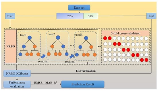
Figure 9.
Flowchart of the NRBO-XGBoost model.
2.4.4. 5-Fold Cross-Validation
In traditional machine learning model evaluations, test errors often exhibit randomness, leading to unstable results [54]. In this research, a 5-fold cross-validation approach was applied by randomly shuffling the samples and evenly dividing them into 5 subsets. In each iteration, 4 of the 5 subsets were allocated for training, while the remaining 1 was designated for model testing and evaluation. After 5 iterations, the average prediction error was calculated as the final evaluation metric. This method makes full use of the samples, so that each sample can participate in different combinations of training and testing, effectively avoiding overfitting or underfitting.
2.4.5. Model Accuracy Evaluation
In this study, the coefficient of determination (R2), mean absolute error (MAE), and root mean square error (RMSE) served as metrics to assess the model’s accuracy. R2 represents the level of fit between the predicted and actual values. MAE represents the prediction error, with a smaller MAE indicating better model performance. RMSE measures the degree of data dispersion, with a smaller value suggesting closer agreement between predictions and observations [55]. The formula is as follows:
In these equations, n represents the sample size; represents the observed value of the i sample; is the predicted value of the sample; and represents the mean of all observed values.
3. Results and Analysis
3.1. Factor Selection
To enhance computational efficiency and minimize data redundancy, this study applied Pearson correlation analysis to explore the associations linking the characteristic parameters of the reflected signal (frequency, amplitude, phase, NMRI, and Heff), key climate factors (average temperature, daily rainfall, cumulative precipitation, and evaporation), and SMC. This analysis aimed to identify the primary factors influencing the accuracy of SMC inversion. Figure 10 presents the correlation analysis results for the P038, P389, P309, P472, P742, and Bkap sites, displayed sequentially by row and column. The bubble diameter (the larger the diameter, the stronger the correlation) and the chromatic gradient (cold tones are negatively correlated; warm tones are positively correlated, and the darker the color, the stronger the correlation) are used to quantify the correlation. Significance levels are indicated using plus (*) markers.
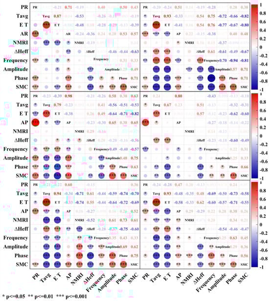
Figure 10.
Pearson correlation coefficients between each factor and SMC at different sites. Cool color represents a negative correlation, while warm color represents a positive correlation.
Among the characteristic parameters of the reflected signal, both phase and amplitude exhibit a strong positive correlation with the SMC at each site, while Heff shows a significant negative correlation with SMC [39]. NMRI shows a weak correlation with SMC, mainly because of its strong correlation with VMC [45,56]. The correlation between evaporation and daily average temperature with SMC is relatively similar, with evaporation at the P472 site playing a more dominant role. Both daily rainfall and cumulative rainfall show a positive correlation with SMC, with cumulative rainfall being more significant across the sites.
3.2. Soil Moisture Inversion Results
3.2.1. SMC Inversion Results Based on ∆φ, ∆Heff, and Amplitude
SMC inversion based on ∆φ, ∆Heff, and amplitude shows that, due to the combined effects of system errors and environmental factors, the relationship between each individual feature and SMC is not strictly linear (Figure 11). Among these, ∆φ shows the highest correlation with SMC [57]. However, the inversion results still exhibit significant discrepancies, particularly during and after rainfall events. Next, ∆Heff, which represents changes in the signal penetration depth, shows varying correlations with SMC at different depths. The correlation between amplitude and SMC is the lowest, resulting in the poorest inversion performance. The modeling and validation phase revealed that single-parameter inversion has limited capability to track the dynamic changes in SMC, with significant error fluctuations. Therefore, relying solely on a single feature for SMC inversion often fails to achieve sufficient accuracy.
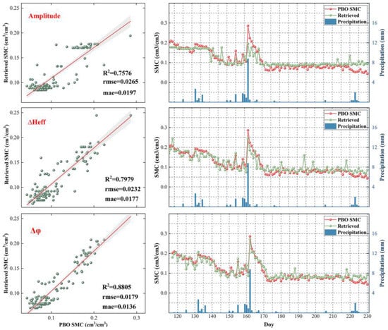
Figure 11.
Single-factor SMC inversion results for station P389. The left graph shows the linear fit of observed and predicted values for amplitude, ∆Heff, and ∆φ. In this graph, the green dots represent individual soil samples, the red line is the regression line, and the gray shadow indicates the 95% confidence interval. The right graph compares the observed values (red circles) with the predicted values (green circles).
3.2.2. SMC Inversion Optimization Based on Multi-Factor Dataset
A multi-factor dataset, selected based on Pearson correlation analysis, served as the foundation for constructing the SMC inversion model. To further evaluate model performance under different variable combinations, three variable combination schemes were designed using the P389 station as an example: Scheme 1: Evaporation, daily rainfall, amplitude, Heff, delayed phase, and frequency; Scheme 2: Average temperature, cumulative rainfall, amplitude, Heff, delayed phase, and frequency; and Scheme 3: Evaporation, cumulative rainfall, amplitude, Heff, delayed phase, and frequency. Figure 12 shows that Scheme 3 achieved the best performance, with R2 = 0.98, RMSE = 0.0056, and MAE = 0.0025. Compared to Scheme 1, R2 improved by 0.91%, while MAE and RMSE decreased by 0.0006 and 0.0019, respectively, demonstrating that cumulative rainfall is more effective than daily rainfall in reflecting changes in SMC over a period following rainfall. Compared to Scheme 2, R2 increased by 1.4%, and MAE and RMSE decreased by 62% and 39%, respectively, indicating that evaporation is a more direct indicator of the impact of climate change on SMC than average temperature. Compared to the single-parameter model, the multi-factor model improved R2 by 11.36%, and reduced MAE and RMSE by 0.0111 and 0.0123, respectively. These results confirm that the multi-factor SMC inversion method can enhance the stability of the model (Figure 11 and Figure 12).
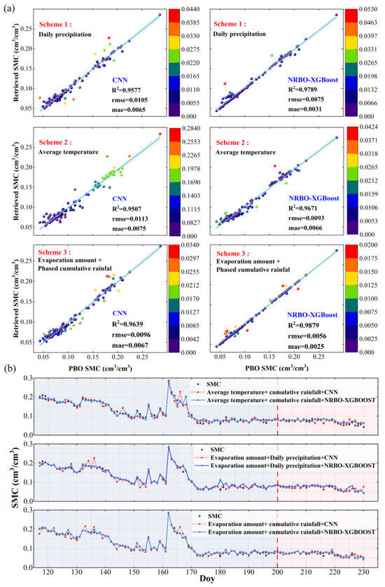
Figure 12.
Multi-factor SMC inversion results for station P389. (a) Linear fit of observed and predicted values for three schemes, with colored dots indicating the degree of deviation from the observed SMC, where redder colors represent a greater deviation. The shaded area represents the 95% confidence interval. (b) Comparison between the observed and predicted values.
3.2.3. SMC Inversion Results Using Multiple Features Under Different Vegetation Cover Types
To further validate the general applicability of the multi-factor SMC inversion model, SMC inversion experiments were conducted at six sites with different vegetation cover types. Figure 13 illustrates the model’s predicted values and the corresponding SMC reference values. The predicted values show strong temporal synchronization with the observed data at all sites, particularly demonstrating high accuracy in monitoring soil moisture responses after precipitation events. To further assess the model’s predictive performance, the residual values for the selected sites were calculated, and the residual plots are presented in Figure 14.
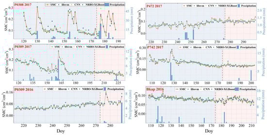
Figure 13.
Comparison of predicted values from each model with the observed SMC values (gray for the training set, pink for the validation set). Red represents the observed SMC values, blue represents the Libsvm predicted values, yellow represents the CNN predicted values, and green represents the NRBO-XGBoost predicted values. The bar chart shows rainfall.
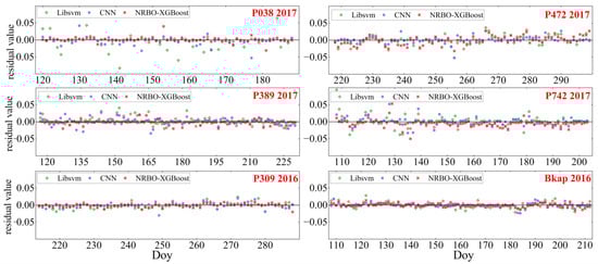
Figure 14.
Residual plot of the model’s predicted values versus the reference SMC values. The rhombus, square, and asterisk are the residuals of Libsvm, CNN, and NRBO-XGBoost models, respectively.
Among the six SMC inversion sites, the grassland (P038) and open shrubland (P389) sites exhibited higher inversion accuracy, whereas the inversion accuracy for the shrub–grassland (P309) and cropland (P742) areas were somewhat lower. The lowest inversion accuracy was observed at the forest–shrub grassland (P472) and bare-soil site (Bkap) [58]. Additionally, the NRBO-XGBoost and CNN models produced smaller soil moisture prediction residuals than the SVR model. Statistical results are provided in Table 4 for a clearer insight into model performance.
Table 4.
Inversion accuracy of each site.
4. Discussion
4.1. The Impact of Different Vegetation Cover on SMC Retrieval Accuracy and Mechanisms
The correlation analysis indicated a reduction in the amplitude and SMC correlation coefficient at the and P472 sites, with values around 0.3. Data analysis showed that the SMC at both sites fluctuated around 0.1 cm3/cm3, consistent with the correlation pattern between surface amplitude and SMC in heterogeneous soils proposed by Jin (where the correlation weakens when SMC < 0.1 cm3/cm3) [22]. However, despite the SMC at the P309 site also being below this threshold, a significant positive correlation of up to 0.7 is observed (Figure 15). A comparison of vegetation parameters reveals that the site’s NDVI > 0.4 aligns with the vegetation canopy effect on GNSS-R signal amplitude attenuation proposed by Li [56], confirming that surface vegetation is the main factor driving the variability in the relationship between amplitude and SMC.
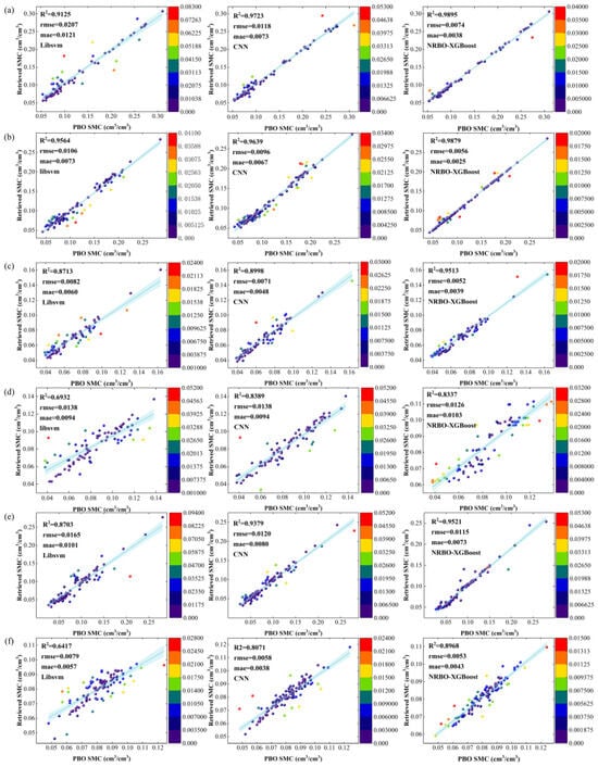
Figure 15.
Linear fitting plots of measured versus predicted SMC values at six sites using the three models. Color indicates the degree of deviation between measured and predicted values. Note: (a) grassland (b) open shrubland (c) savannas (d) woody savannas (e) cultivated land (f) barren land.
The multi-factor model significantly enhanced the accuracy of SMC inversion (Figure 11, Figure 12 and Figure 15). However, despite the favorable GNSS-IR observation conditions at the Bkap station (bare land)—such as no occlusions and an open field of view—the inversion accuracy remained relatively low, with R2 = 0.89 (Figure 15f). This phenomenon can be attributed to the high sensitivity of GNSS signals to soil dielectric constants (positively correlated with moisture and negatively correlated with temperature [59]). As the station is located in a desert climate zone with sparse vegetation and a surface roughness prone to wind erosion, the reflected signal remains unstable over time [60]. The P472 (woody savannas) station experiences significant interference in reflection signals due to the uneven distribution of the vegetation canopy and low incidence angles (5–25°) [61]. Experiments show that the multi-factor SMC inversion model performs better for low-growing and sparse vegetation, while complex vegetation and bare land (near desert areas) are more susceptible to interference from climatic and natural conditions.
4.2. Impact of Model Selection on SMC Inversion Results
SVR achieves optimal regression by mapping data to a higher-dimensional space. The CNN completes the regression through feature extraction and dimensionality reduction, followed by the output of the feature map through the fully connected layer [45,55]. The NRBO-XGBoost model utilizes second-order derivatives (Hessian matrix) for numerical optimization, enabling automatic hyperparameter selection and tuning [45]. A comparison of the MAE for the three models at six stations (Figure 16) shows that NRBO-XGBoost exhibits the lowest and most stable error distribution. Li compared the performance of RF and XGBoost in SMC inversion on the Qinghai-Tibet Plateau (R2 = 0.83 and 0.85, respectively), further confirming the stability of the XGBoost model [62]. CNN performs next in line, with Xian using CNN for SMC inversion, achieving an R2 greater than 0.95, which is similar to the results obtained for the P038 and P389 stations [39]. On the other hand, SVR exhibits a significant deviation in error. Zhang used the SVR, BPNN, and MARS models for SMC inversion at the P041 station, with SVR showing the poorest performance [29]. It is evident that the NRBO-XGBoost model is more effective at capturing the complex interactions between environmental factors and SMC.
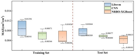
Figure 16.
MAE box plots based on three models in the training set and test set of six sites.
4.3. Research Constraints and Future Directions
Due to the long monitoring period of the GNSS-IR technology, factors such as vegetation cover type and climate change can affect data quality. To overcome these challenges, this study developed a multi-factor SMC inversion model, which exhibited strong robustness and reliability under various environmental conditions, offering a valuable reference for future SMC inversion research. However, this research overlooked the influence of soil type and surface roughness on inversion accuracy. Future work will involve more in-depth investigations to improve the model’s stability.
The SMC monitoring range of a single GNSS station is limited to approximately 1000 square meters around the site. While it provides valuable local data, achieving large-scale, high-precision SMC monitoring remains challenging. In contrast, InSAR technology offers significant advantages in spatial resolution, enabling large-area observations. However, its temporal resolution is constrained by the revisit cycle, making it challenging to capture rapid soil moisture dynamics. Based on this, future research could integrate GNSS’s fine temporal resolution with InSAR’s extensive spatial coverage to generate SMC datasets with enhanced spatiotemporal resolution.
5. Conclusions
As an essential indicator of the water cycle, high spatiotemporal resolution SMC monitoring has important applications in precision agriculture and environmental protection. Given the limitations of GNSS-IR-based SMC inversion in data utilization and across different scenarios, and considering the effects of vegetation and meteorological factors, a multi-factor fusion model for SMC inversion was proposed. By integrating vegetation error correction, cumulative rainfall, average evaporation rate, and multi-GNSS multi-satellite data, a comprehensive multi-factor database was established. Three distinct machine learning algorithms were developed for SMC inversion: SVR, CNN, and NRBO-XGBoost. The experimental analysis led to the following conclusions:
Compared with traditional models, the multi-factor inversion model demonstrated significant performance improvements, with R2 increasing by 8.2–24.1%, RMSE decreasing by 75–84.7%, and MAE reducing by 86.1–91.1%. At the same time, the model performed well across different sites, enhancing its overall applicability.
- (1)
- Comprehensive analysis of different land cover types revealed that SMC inversion demonstrated significantly higher accuracy in grassland and open shrubland areas compared to other vegetation types.
- (2)
- Based on MP1, the NMRI exhibited a significant correlation with NDVI, which supports correction of distortions in the reflected signal’s amplitude and phase induced by VMC. However, errors increase when using the delayed phase to invert SMC after rainfall, highlighting the need to consider the influence of rainfall on the delayed phase.
- (3)
- The GNSS-IR technology was used to estimate SMC across different land types, and the performance of three models—SVR, CNN, and NRBO-XGBoost—was compared. The results showed that the NRBO-XGBoost model demonstrated higher stability.
The multi-factor SMC inversion model proposed in this study demonstrated robust performance and reliability under various environmental conditions, providing a valuable reference for future SMC inversion research. However, this study did not account for the effects of soil type and surface roughness on inversion results. Future research will aim to explore how soil type and surface roughness affect inversion accuracy, with the goal of developing a more robust and stable inversion model.
Author Contributions
Conceptualization, J.Y. and X.Y.; methodology, X.Y.; validation, G.L., W.M., and Q.L.; formal analysis, Y.Y.; data curation, J.L.; writing—original draft preparation, Y.Y.; writing—review and editing, M.S. and Y.Y.; visualization, M.S. All authors have read and agreed to the published version of the manuscript.
Funding
This work was supported by the following grants: the major science and technology project of Gansu Province (24ZD13NA019), the Central Guide Local Science and Technology Development Special Funds (24ZYQA023), the National Natural Science Foundation of China (42461060; 42307564), the Gansu Province Provincial-Level Key R&D Special Project for Ecological Civilization Construction (24YFFA059; 24YFFA056), and the Gansu Province Department of Education Industry Support Program Project (2025CYZC-042; 2022CYZC-41).
Data Availability Statement
The GNSS station data were provided by the United States Plate Boundary Observatory (PBO) monitoring program (https://data.unavco.org/archive/gnss/rinex/, accessed on 14 April 2024). The SMC reference data and rainfall data were obtained from the International Soil Moisture Network (https://ismn.earth/en/dataviewer/, accessed on 14 April 2024).
Acknowledgments
The authors sincerely appreciate the constructive comments provided by the anonymous reviewers and the members of the editorial team. Additionally, they would like to thank the Plate Boundary Observatory (PBO) in the United States for providing GNSS data, and the International Soil Moisture Network for offering rainfall and SMC data, both of which were crucial for supporting this research.
Conflicts of Interest
The authors declare no conflicts of interest.
Abbreviation List
| Abbreviation | Full Form |
| AR | Accumulated Rainfall |
| AAF | Amplitude Attenuation Factor |
| CNN | Convolutional Neural Networks |
| DEM | Digital Elevation Model |
| GNSS | Global Navigation Satellite System |
| GNSS-IR | Global Navigation Satellite System Interferometric Reflection |
| GPS | Global Positioning System |
| NDVI | Normalized Difference Vegetation Index |
| NMRI | Normalized Microwave Reflection Index |
| NRBO | Newton–Raphson-Based Optimize |
| NRSR | Newton–Raphson Search Rule |
| PR | Precipitation |
| SMC | Soil Moisture Content |
| SNR | Signal-to-Noise Ratio |
| SVR | Support Vector Regression |
| Tavg | Average Temperature |
| VWC | Vegetation Moisture Content |
| XGBoost | Extreme Gradient Boosting |
| GEE | Google Earth Engine |
| ESA | European Space Agency |
| ET | Evapotranspiration |
Symbol Nomenclature
| Symbol | Description |
| Ad | direct signal |
| Ar | reflected signal |
| bias term | |
| CART | classification and regression tree |
| dim | problem dimension |
| E[L(X,θ)] | expected value of the objective function, accounting for noise and uncertainty |
| f | frequencies |
| H | antenna height |
| Heff | effective reflective height |
| K (xi + xj) | kernel function |
| L(X,θ) | loss function of XGBoost |
| lb | lower bounds |
| M j | input mapping layers |
| MP1 | pseudorange multipath error of the L1 carrier |
| MAE | mean absolute error |
| P1 | pseudorange observation on the L1 carrier |
| R2 | coefficient of determination |
| R(θ) | regularization term |
| rand | random number between 0 and 1 |
| randn | normally distributed random number with mean 0 and variance 1 |
| RBF | radial basis function |
| RMSE | root mean squared error |
| SNRr | residual sequence of low elevation angle containing reflection information |
| TAO | trap avoidance operator |
| ub | upper bounds |
| weight matrix of the j convolutional kernel in the i layer | |
| ‖w‖2 | sum of the squares of the weight vector |
| input to the j convolutional kernel of the I layer, also the output of the I − 1 layer | |
| convolution kernel | |
| XI+1(j) | value of the j output neuron in the I + 1 layer |
| position of the j dimension in the population | |
| optimal set of hyperparameters derived from NRBO optimization | |
| θ | satellite elevation angle |
| λ | wavelength |
| ξ | slack variable |
| ϵ | error tolerance |
| φ | delay phase |
References
- Farrell, M.; Leizica, E.; Gili, A.; Noellemeyer, E. Identification of management zones with different potential moisture availability for sustainable intensification of dryland agriculture. Precis. Agric. 2023, 24, 1116–1131. [Google Scholar] [CrossRef]
- Zhu, M.K.; Kong, F.L.; Li, Y.; Li, M.M.; Zhang, J.L.; Xi, M. Effects of moisture and salinity on soil dissolved organic matter and ecological risk of coastal wetland. Environ. Res. 2020, 187, 109659. [Google Scholar] [CrossRef]
- Hauser, M.; Orth, R.; Seneviratne, S.I. Investigating soil moisture—climate interactions with prescribed soil moisture experiments: An assessment with the Community Earth System Model (version 1.2). Geosci. Model Dev. 2017, 10, 1665–1677. [Google Scholar] [CrossRef]
- Gupta, S.K.; Singh, S.K.; Kanga, S.; Kumar, P.; Meraj, G.; Sahariah, D.; Debnath, J.; Chand, K.; Sajan, B.; Singh, S. Unearthing India’s soil moisture anomalies: Impact on agriculture and water resource strategies. Theor. Appl. Climatol. 2024, 155, 7575–7590. [Google Scholar] [CrossRef]
- Piccini, C.; Metzger, K.; Debaene, G.; Stenberg, B.; Götzinger, S.; Borůvka, L.; Sandén, T.; Bragazza, L.; Liebisch, F. In-field soil spectroscopy in Vis–NIR range for fast and reliable soil analysis: A review. Eur. J. Soil Sci. 2024, 75, e13481. [Google Scholar] [CrossRef]
- Muzylev, E.L. Utilization of Remote Sensing Data in the Simulation of the Water and Heat Regime of Land Areas: A Review of Publications. Water Resour. 2023, 50, 709–731. [Google Scholar] [CrossRef]
- Kandala, R.; Franssen, H.H.; Chaudhuri, A.; Sekhar, M. The value of soil temperature data versus soil moisture data for state, parameter, and flux estimation in unsaturated flow model. Vadose Zone J. 2024, 23, e20298. [Google Scholar] [CrossRef]
- Yan, G.X.; Bore, T.; Schlaeger, S.; Scheuermann, A.; Li, L. Dynamic effects in soil water retention curves: An experimental exploration by full-scale soil column tests using spatial time-domain reflectometry and tensiometers. Acta Geotech. 2024, 19, 7517–7543. [Google Scholar] [CrossRef]
- Bore, T.; Yan, G.; Mishra, P.N.; Brierre, T.; Placencia-Gómez, E.; Revil, A.; Wagner, N. A flow through coaxial cell to investigate high frequency broadband complex permittivity: Design, calibration and validation. Measurement 2024, 237, 115198. [Google Scholar] [CrossRef]
- Abdulraheem, M.I.; Chen, H.; Li, L.; Moshood, A.Y.; Zhang, W.; Xiong, Y.; Zhang, Y.; Taiwo, L.B.; Farooque, A.A.; Hu, J. Recent Advances in Dielectric Properties-Based Soil Water Content Measurements. Remote Sens. 2024, 16, 1328. [Google Scholar] [CrossRef]
- Akash, M.; Kumar, P.M.; Bhaskar, P.; Deepthi, P.R.; Sukhdev, A. Review of estimation of soil moisture using active microwave remote sensing technique. Remote Sens. Appl. Soc. Environ. 2024, 33, 101118. [Google Scholar] [CrossRef]
- Cheng, T.; Hong, S.; Huang, B.; Qiu, J.; Zhao, B.; Tan, C. Passive Microwave Remote Sensing Soil Moisture Data in Agricultural Drought Monitoring: Application in Northeastern China. Water 2021, 13, 2777. [Google Scholar] [CrossRef]
- Li, M.; Yan, Y. Comparative Analysis of Machine-Learning Models for Soil Moisture Estimation Using High-Resolution Remote-Sensing Data. Land 2024, 13, 1331. [Google Scholar] [CrossRef]
- Li, S.; Zhu, P.; Song, N.; Li, C.; Wang, J. Regional Soil Moisture Estimation Leveraging Multi-Source Data Fusion and Automated Machine Learning. Remote Sens. 2025, 17, 837. [Google Scholar] [CrossRef]
- Lu, H.; Tian, J. Integrating Machine Learning with Data Assimilation for High Resolution Soil Moisture Estimation. In Proceedings of the IGARSS 2024—2024 IEEE International Geoscience and Remote Sensing Symposium, Athens, Greece, 7–12 July 2024; pp. 5179–5182. [Google Scholar] [CrossRef]
- Wang, X.L.; Song, M.F.; He, X.F.; Zhang, T.T. Enhancing sea level inversion accuracy with a novel phase-based error correction method and multi-GNSS combination approach. GPS Solut. 2025, 29, 34. [Google Scholar] [CrossRef]
- Ding, R.; Zheng, N.; Stienne, G.; He, J.; Zhang, H.; Liu, X. A High Spatiotemporal Resolution Snow Depth Inversion Solution with Multi-GNSS-IR in Complex Terrain. J. Sel. Top. Appl. Earth Obs. Remote Sens. 2024, 17, 14874–14893. [Google Scholar] [CrossRef]
- Purnell, D.; Dabboor, M.; Matte, P.; Peters, D.; Anctil, F.; Ghobrial, T. Observations of River Ice Breakup Using GNSS-IR, SAR and Machine Learning. IEEE Trans. Geosci. Remote Sens. 2024, 62, 5800613. [Google Scholar] [CrossRef]
- Yang, C.; Mao, K.; Guo, Z.; Shi, J.; Bateni, S.M.; Yuan, Z. Review of GNSS-R Technology for Soil Moisture Inversion. Remote Sens. 2024, 16, 1193. [Google Scholar] [CrossRef]
- Larson, K.M.; Small, E.E.; Gutmann, E.; Bilich, A.; Axelrad, P.; Braun, J. Using GPS multipath to measure soil moisture fluctuations: Initial results. GPS Solut. 2008, 12, 173–177. [Google Scholar] [CrossRef]
- Pierdicca, N.; Guerriero, L.; Giusto, R.; Brogioni, M.; Egido, A. SAVERS: A Simulator of GNSS Reflections from Bare and Vegetated Soils. IEEE Trans. Geosci. Remote Sens. 2014, 52, 6542–6554. [Google Scholar] [CrossRef]
- Chew, C.C.; Small, E.E.; Larson, K.M.; Zavorotny, V.U. Effects of Near-Surface Soil Moisture on GPS SNR Data: Development of a Retrieval Algorithm for Soil Moisture. IEEE Trans. Geosci. Remote Sens. 2013, 52, 537–543. [Google Scholar] [CrossRef]
- Tabibi, S.; Nievinski, F.G.; Dam, T.V.; João, F.G. Assessment of modernized GPS L5 SNR for ground-based multipath reflectometry applications. Adv. Space Res. 2015, 55, 1104–1116. [Google Scholar] [CrossRef]
- Han, M.; Zhu, Y.; Yang, D.; Hong, X.; Song, S. A Semi-Empirical SNR Model for Soil Moisture Retrieval Using GNSS SNR Data. Remote Sens. 2018, 10, 280. [Google Scholar] [CrossRef]
- Liang, Y.; Ren, C.; Huang, Y. Research on multi-satellites fusion inversion model of soil moisture based on sliding window. In Proceedings of the China Satellite Navigation Conference (CSNC) 2018, Harbin, China, 23–25 May 2018; Sun, J., Yang, C., Guo, S., Eds.; Springer: Singapore, 2018; Volume I, pp. 85–95. [Google Scholar] [CrossRef]
- Jiang, L.L.; Yang, L.; Han, M.; Hong, X.B.; Sun, B.; Liang, Y. Soil moisture inversion method based on GNSS-IR dual frequency data fusion. J. Beijing Univ. Aeronaut. Astronaut. 2019, 45, 1248–1255. [Google Scholar] [CrossRef]
- Nie, S.; Wang, Y.; Tu, J.; Li, P.; Xu, J.; Li, N.; Wang, M.; Huang, D.; Song, J. Retrieval of Soil Moisture Content Based on Multisatellite Dual-Frequency Combination Multipath Errors. Remote Sens. 2022, 14, 3193. [Google Scholar] [CrossRef]
- Zhu, Y.; Shen, F.; Sui, M.; Cao, X. Effects of Parameter Selections on Soil Moisture Retrieval Using GNSS-IR. IEEE Access 2020, 8, 211784–211793. [Google Scholar] [CrossRef]
- Lv, J.; Zhang, R.; Tu, J.; Liao, M.; Pang, J.; Yu, B.; Li, K.; Xiang, W.; Fu, Y.; Liu, G. A GNSS-IR Method for Retrieving Soil Moisture Content from Integrated Multi-Satellite Data That Accounts for the Impact of Vegetation Moisture Content. Remote Sens. 2021, 13, 2442. [Google Scholar] [CrossRef]
- Ding, Q.; Liang, Y.; Liang, X.; Ren, C.; Yan, H.; Liu, Y.; Zhang, Y.; Lu, X.; Lai, J.; Hu, X. Soil Moisture Retrieval Using GNSS-IR Based on Empirical Modal Decomposition and Cross-Correlation Satellite Selection. Remote Sens. 2023, 15, 3218. [Google Scholar] [CrossRef]
- Zhang, X.; Nie, S.; Zhang, C.; Zhang, J.; Cai, H. Soil moisture estimation based on triple-frequency multipath error. Int. J. Remote Sens. 2021, 42, 5953–5968. [Google Scholar] [CrossRef]
- Wei, H.; Yang, X.; Pan, Y.; Shen, F. GNSS-IR Soil Moisture Inversion Derived from Multi-GNSS and Multi-Frequency Data Accounting for Vegetation Effects. Remote Sens. 2023, 15, 5381. [Google Scholar] [CrossRef]
- Ma, J.J.; Liang, Y.J.; Cheng, B.; Hu, X.M.; Ren, C.; Yang, M.M.; Huang, Y.B.; Liang, C.W.; Guo, X. A synchronous retrieval method of vegetation water content and soil moisture based on GNSS-IR and multi-source data fusion. J. Spat. Sci. 2025, 70, 161–181. [Google Scholar] [CrossRef]
- Pan, Y.L.; Ren, C.; Liang, Y.J.; Zhang, Z.G.; Shi, Y.J. Inversion of surface vegetation water content based on GNSS-IR and MODIS data fusion. Satell. Navig. 2020, 1, 21. [Google Scholar] [CrossRef]
- Ding, R.; Zheng, N.; Zhang, H.; Zhang, H.; Lang, F.; Ban, W. A Study of GNSS-IR Soil Moisture Inversion Algorithms Integrating Robust Estimation with Machine Learning. Sustainability 2023, 15, 6919. [Google Scholar] [CrossRef]
- Zhang, Y.; Bu, J.; Zuo, X.; Yu, K.; Wang, Q.; Huang, W. Vegetation Water Content Retrieval from Spaceborne GNSS-R and Multi-Source Remote Sensing Data Using Ensemble Machine Learning Methods. Remote Sens. 2024, 16, 2793. [Google Scholar] [CrossRef]
- Li, Y.J.; Zhu, M.Y.; Luo, L.Y.; Wang, S.; Chen, C.; Zhang, Z.T.; Yao, Y.F.; Hu, X.T. GNSS-IR dual-frequency data fusion for soil moisture inversion based on Helmert variance component estimation. J. Hydrol. 2024, 631, 130752. [Google Scholar] [CrossRef]
- Huang, C.W.; Liu, L.L.; Lin, M.J.; Huang, Q.W.; Bi, H.H. A GNSS-IR soil moisture inversion method based on the SSA assisted ELM. In Proceedings of the SPIE, International Conference on Remote Sensing and Digital Earth (RSDE 2024), Chengdu, China, 2 January 2025; Volume 13514, pp. 62–67. [Google Scholar] [CrossRef]
- Xian, H.Y.; Shen, F.; Guan, Z.P.; Zhou, F.; Cao, X.Y.; Ge, Y.L. A GNSS-IR soil moisture retrieval method via multi-layer perceptron with consideration of precipitation and environmental factors. GPS Solut. 2024, 28, 122. [Google Scholar] [CrossRef]
- Bilich, A.; Larson, K.M.; Axelrad, P. Modeling GPS phase multipath with SNR: Case study from the Salar de Uyuni, Boliva. J. Geophys. Res. Solid Earth 2008, 113, 0148–0227. [Google Scholar] [CrossRef]
- Chew, C.; Small, E.E.; Larson, K.M. An algorithm for soil moisture estimation using GPS-interferometric reflectometry for bare and vegetated soil. GPS Solut. 2016, 20, 525–537. [Google Scholar] [CrossRef]
- Roussel, N.; Frappart, F.; Ramillien, G.; Darrozes, J.; Desjardins, C.; Gegout, P.; Pérosanz, F.; Biancale, R. Simulations of direct and reflected wave trajectories for ground-based GNSS-R experiments. Geosci. Model Dev. 2014, 7, 2261–2279. [Google Scholar] [CrossRef]
- Roussel, N.; Frappart, F.; Ramillien, G.; Darrozes, J.; Baup, F.; Lestarquit, L. Detection of soil moisture variations using GPS and GLONASS SNR data for elevation angles ranging from 2° to 70°. IEEE J. Sel. Top. Appl. Earth Obs. Remote Sens. 2016, 9, 4781–4794. [Google Scholar] [CrossRef]
- Kim, S.B.; Huang, H.; Liao, T.H.; Colliander, A. Estimating Vegetation Water Content and Soil Surface Roughness Using Physical Models of L-Band Radar Scattering for Soil Moisture Retrieval. Remote Sens. 2018, 10, 556. [Google Scholar] [CrossRef]
- Larson, K.M.; Small, E.E. Normalized Microwave Reflection Index: A Vegetation Measurement Derived from GPS Networks. IEEE J. Sel. Top. Appl. Earth Obs. Remote Sens. 2014, 7, 1501–1511. [Google Scholar] [CrossRef]
- Li, Z.; Liu, F.; Yang, W.; Peng, S.; Zhou, J. A Survey of Convolutional Neural Networks: Analysis, Applications, and Prospects. IEEE Trans. Neural Netw. Learn. Syst. 2022, 33, 6999–7019. [Google Scholar] [CrossRef] [PubMed]
- Cheng, K.; Lu, Z. Active learning Bayesian support vector regression model for global approximation. Inf. Sci. 2021, 544, 549–563. [Google Scholar] [CrossRef]
- Taye, M.M. Theoretical Understanding of Convolutional Neural Network: Concepts, Architectures, Applications, Future Directions. Computation 2023, 11, 52. [Google Scholar] [CrossRef]
- Cong, S.; Zhou, Y. A review of convolutional neural network architectures and their optimizations. Artif. Intell. Rev. 2023, 56, 1905–1969. [Google Scholar] [CrossRef]
- Gopalani, P.; Mukherjee, A. Global convergence of SGD on two layer neural nets, Information and Inference. J. IMA 2025, 14, iaae035. [Google Scholar] [CrossRef]
- Sowmya, R.; Premkumar, M.; Jangir, P. Newton-Raphson-based optimizer: A new population-based metaheuristic algorithm for continuous optimization problems. Eng. Appl. Artif. Intell. 2024, 128, 107532. [Google Scholar] [CrossRef]
- Dong, J.W.; Chen, Y.M.; Yao, B.Y.; Zhang, X.; Zeng, N.F. A neural network boosting regression model based on XGBoost. Appl. Soft Comput. 2022, 125, 109067. [Google Scholar] [CrossRef]
- Li, Y.; Liu, B.; Chai, X.; Guo, F.; Li, Y.; Fu, D. Research on Shallow Water Depth Remote Sensing Based on the Improvement of the Newton–Raphson Optimizer. Water 2025, 17, 552. [Google Scholar] [CrossRef]
- Jung, Y. Multiple predicting K-fold cross-validation for model selection. J. Nonparametric Stat. 2017, 30, 197–215. [Google Scholar] [CrossRef]
- Chicco, D.; Warrens, M.J.; Jurman, G. The coefficient of determination R-squared is more informative than SMAPE, MAE, MAPE, MSE and RMSE in regression analysis evaluation. PeerJ Comput. Sci. 2021, 7, e623. [Google Scholar] [CrossRef] [PubMed]
- Li, J.; Yang, D.K.; Wang, F.; Hong, X.B.; Yang, L. A two-antenna GNSS approach to determine soil moisture content and vegetation growth status. GPS Solut. 2024, 28, 75. [Google Scholar] [CrossRef]
- Jing, L.L.; Wang, N.Z.; Gao, F.; Xu, T.H.; Kong, Y.H.; Wang, L.; Yang, L. A soil moisture retrieval algorithm on bare surface using GNSS-IR technique. Measurement 2025, 249, 117095. [Google Scholar] [CrossRef]
- Li, J.; Yang, D.; Wang, F.; Hong, X. Statistical Analysis of Land-Based GNSS-IR/R Over Bare and Vegetation Surfaces. IEEE Trans. Geosci. Remote Sens. 2024, 62, 75. [Google Scholar] [CrossRef]
- Li, Y.; Xu, T.; Yang, S.; Yu, K.; Chang, X.; Jin, T. A Forward Model and Inversion Algorithm for Near-Surface Soil Moisture Estimation with GNSS Refraction Pattern Technique. IEEE Trans. Geosci. Remote Sens. 2024, 62, 14301119. [Google Scholar] [CrossRef]
- Asgari1, D.; Rahmani, M.; Asgari, J.; Asgarimehr, M.; Wickert, J. Investigation of the Global Influence of Surface Roughness on Space-borne GNSS-R Observations. J. Geophys. Res. Biogeosci. 2025, 130, e2024JG008243. [Google Scholar] [CrossRef]
- Calvet, J.C.; Wigneron, J.P.; Walker, J.; Karbou, F.; Chanzy, A.; Albergel, C. Sensitivity of Passive Microwave Observations to Soil Moisture and Vegetation Water Content: L-Band to W-Band. IEEE Trans. Geosci. Remote Sens. 2011, 49, 1190–1199. [Google Scholar] [CrossRef]
- He, L.; Cheng, Y.; Li, Y.; Li, F.; Fan, K.; Li, Y. An Improved Method for Soil Moisture Monitoring with Ensemble Learning Methods Over the Tibetan Plateau. IEEE J. Sel. Top. Appl. Earth Obs. Remote Sens. 2021, 14, 2833–2844. [Google Scholar] [CrossRef]
Disclaimer/Publisher’s Note: The statements, opinions and data contained in all publications are solely those of the individual author(s) and contributor(s) and not of MDPI and/or the editor(s). MDPI and/or the editor(s) disclaim responsibility for any injury to people or property resulting from any ideas, methods, instructions or products referred to in the content. |
© 2025 by the authors. Licensee MDPI, Basel, Switzerland. This article is an open access article distributed under the terms and conditions of the Creative Commons Attribution (CC BY) license (https://creativecommons.org/licenses/by/4.0/).