Optimization of the Canopy Three-Dimensional Reconstruction Method for Intercropped Soybeans and Early Yield Prediction

 , and
, and
Abstract
1. Introduction
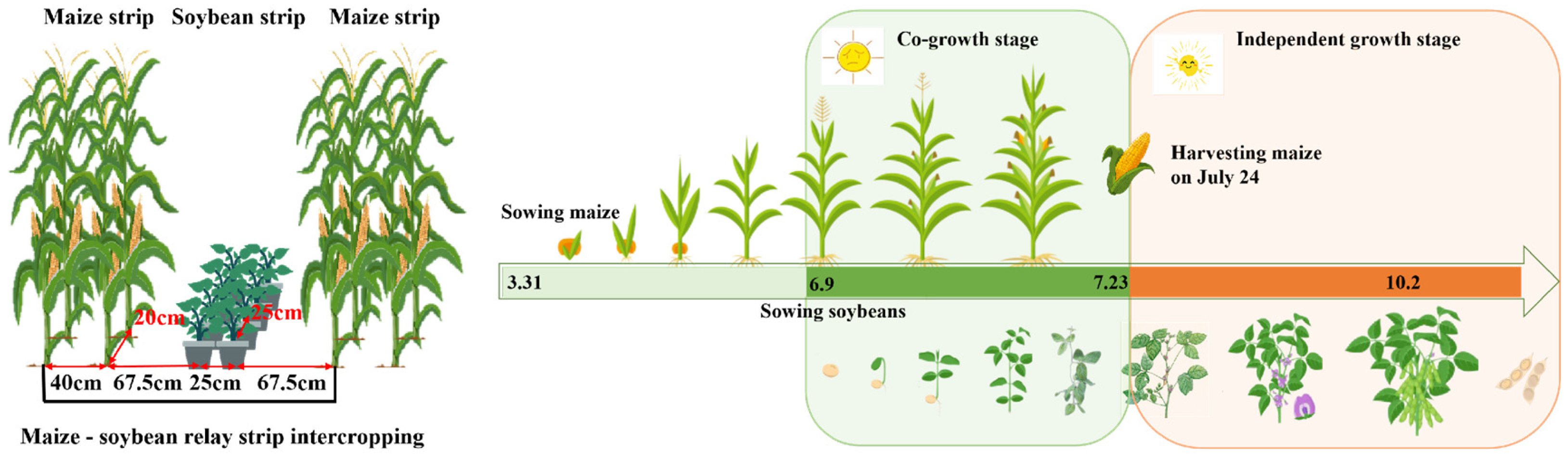
2. Experimental Site and Experimental Design
2.1. High-Throughput Phenotyping Acquisition
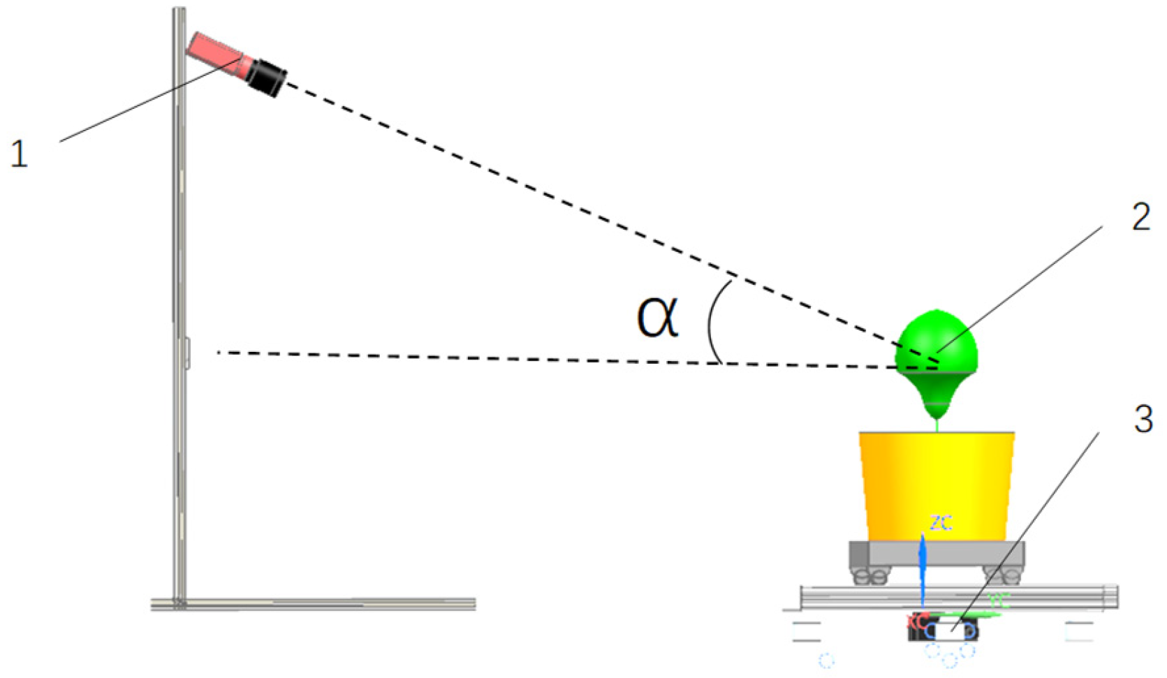
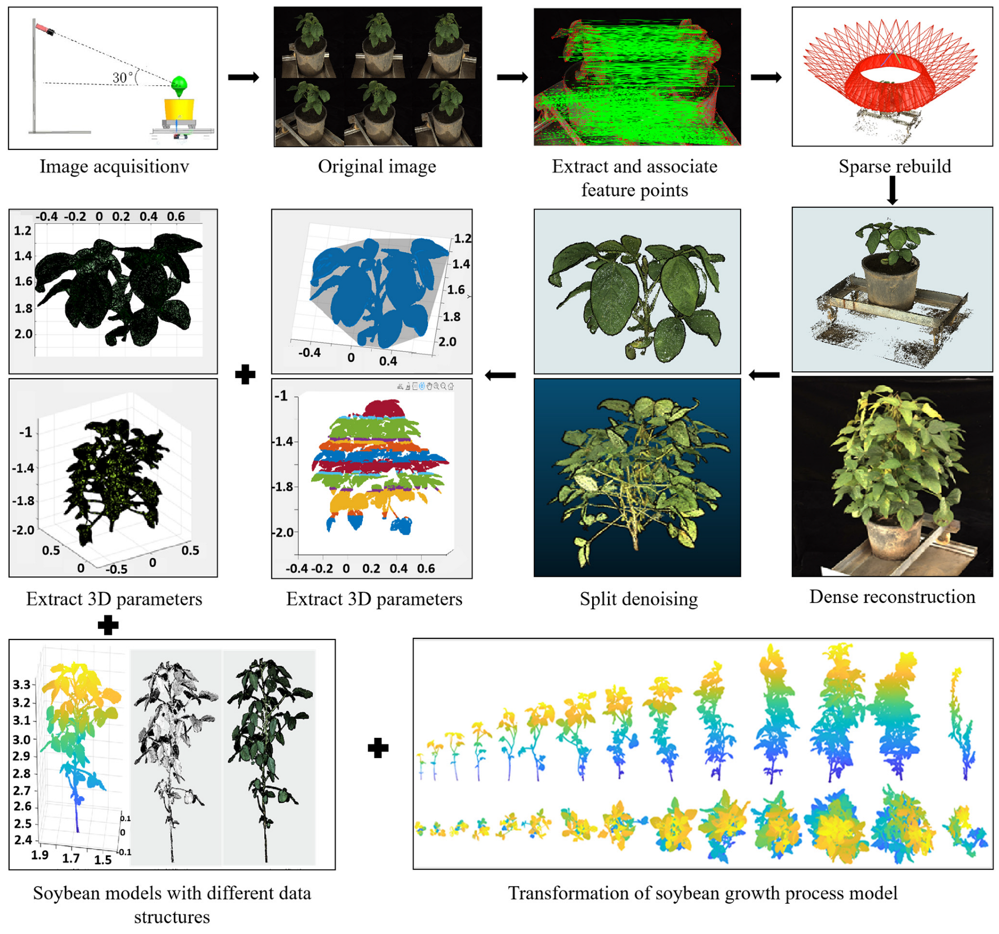
2.1.1. Raw Image Acquisition
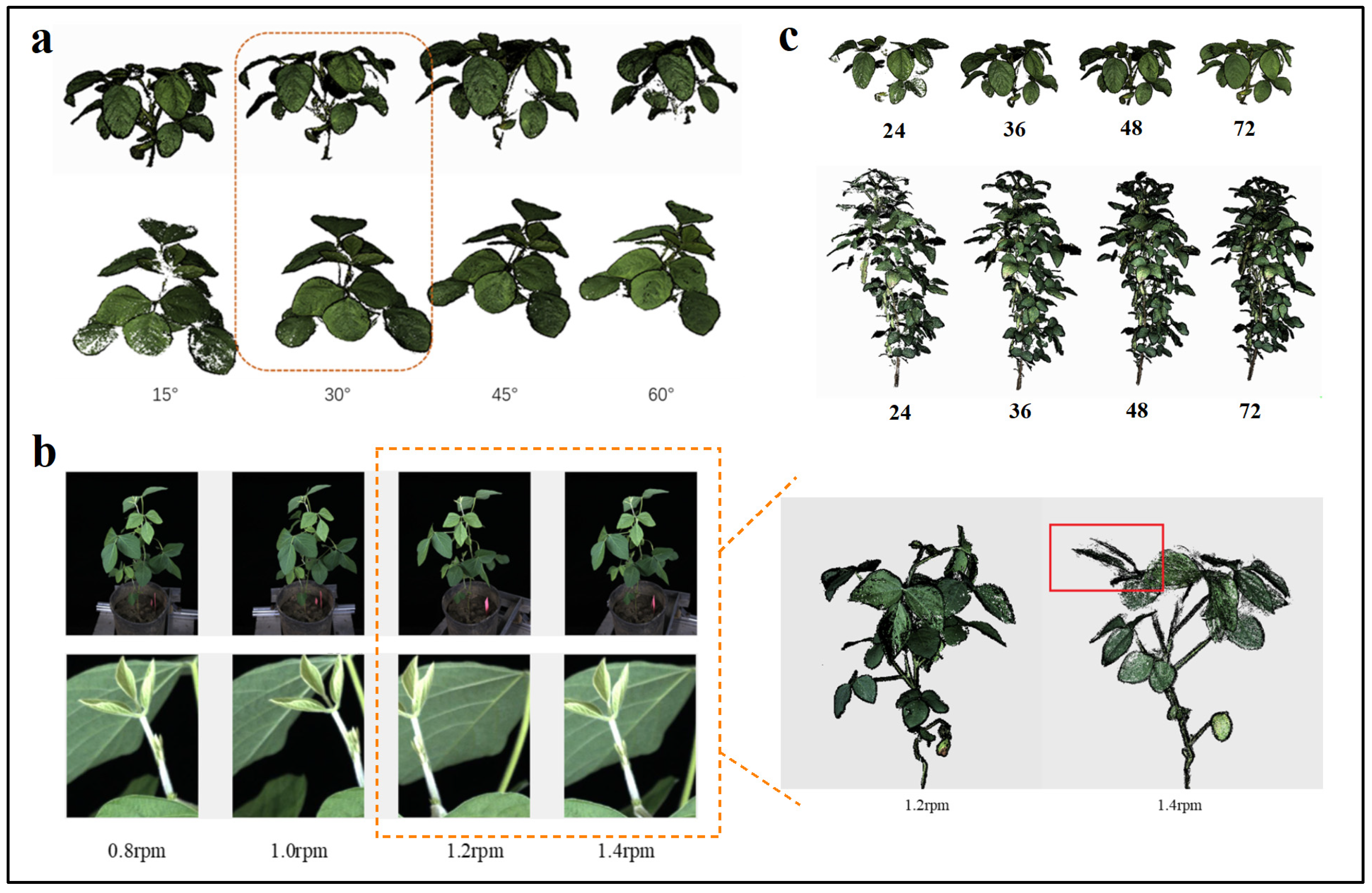
Soybean Plant Image Acquisition Angles
Soybean Plant Rotation Speed
Image Acquisition Quantity
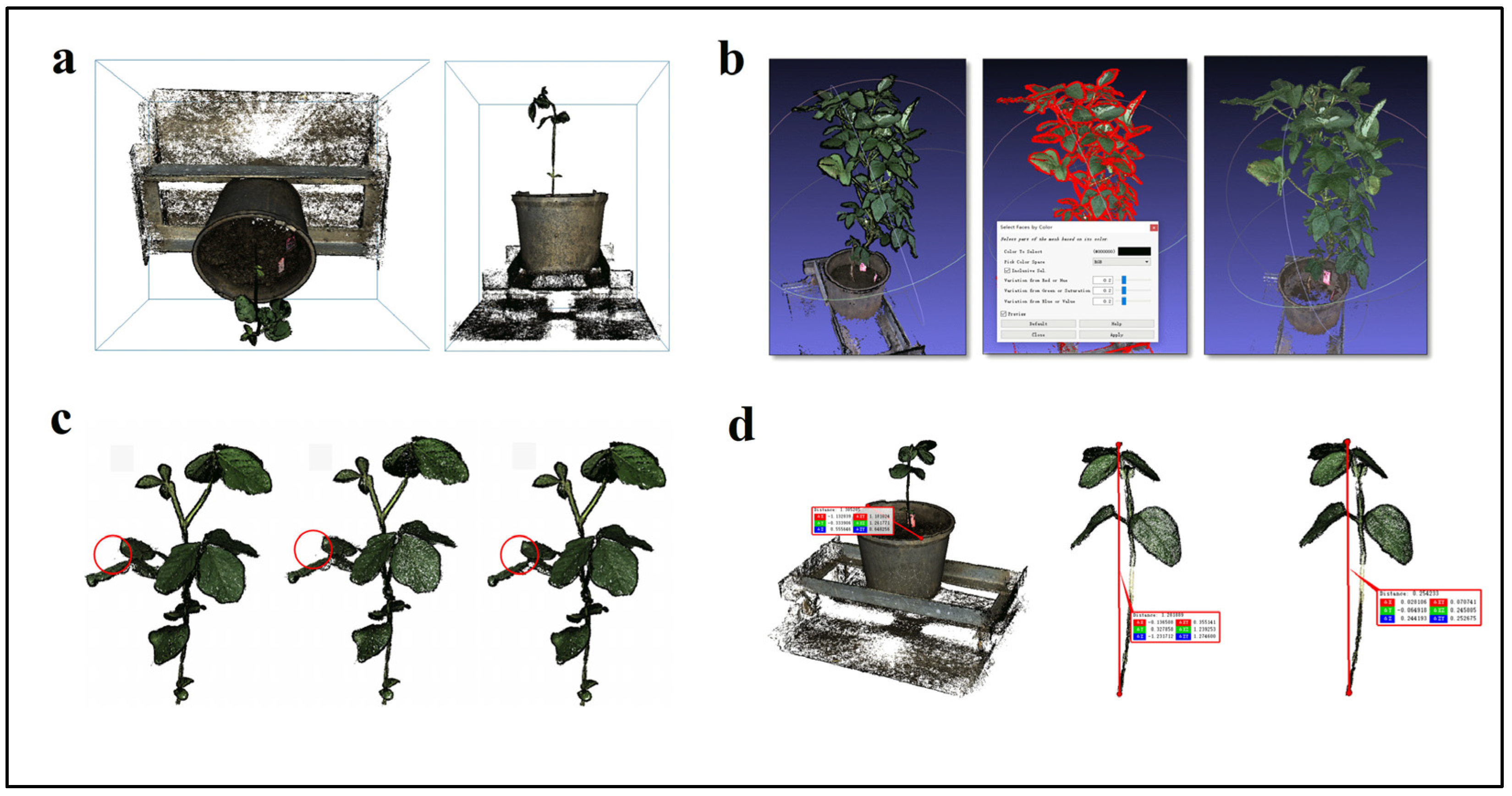
2.1.2. Point Cloud Preprocessing
Spatial Angle Transformation
Point Cloud Segmentation
Point Cloud Denoising
Point Cloud Scaling
2.1.3. Extraction of Image Parameters
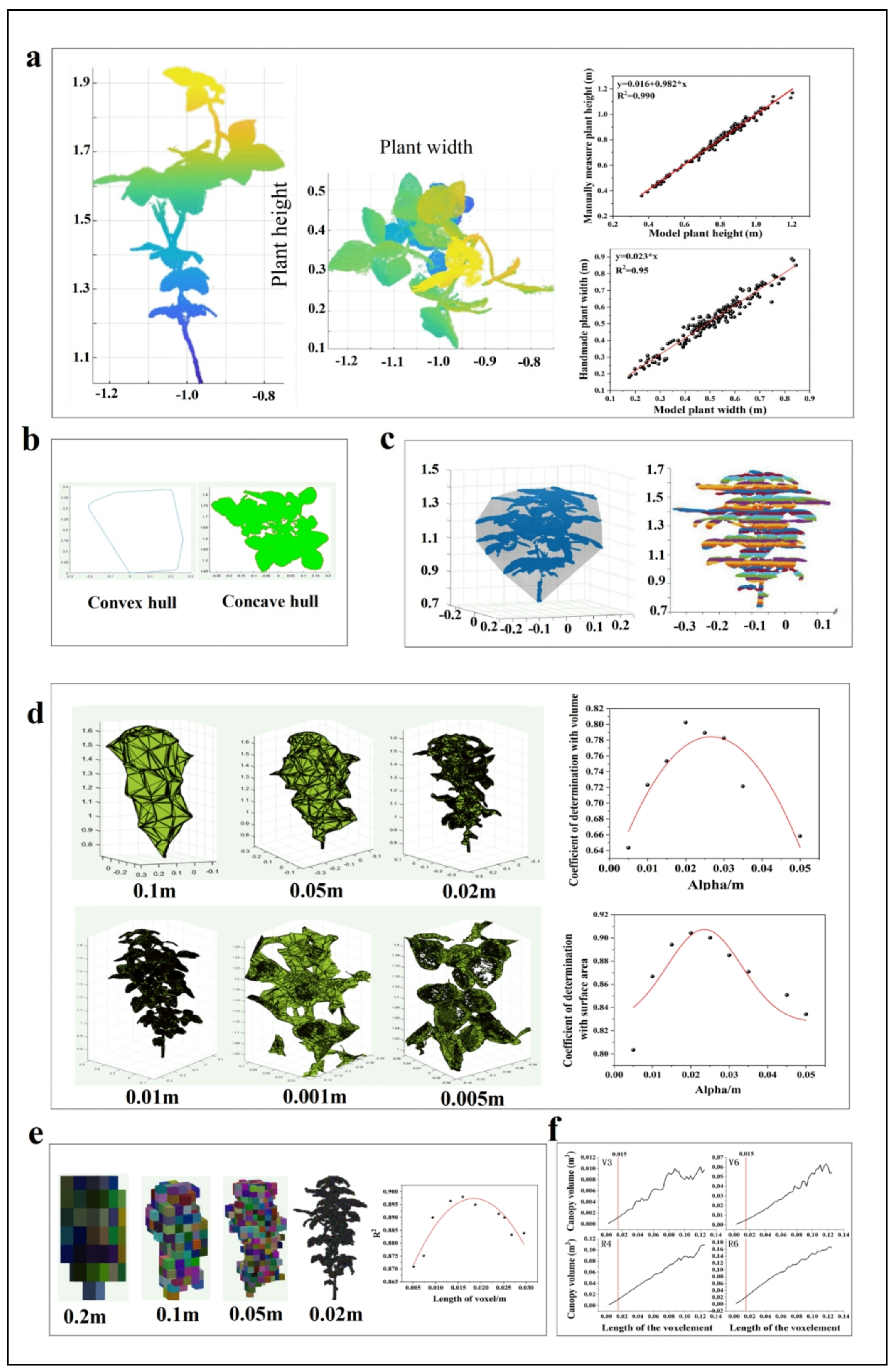
One-Dimensional Parameters
Two-Dimensional Parameters
Three-Dimensional Parameters
2.1.4. High-Throughput Phenotyping Information Acquisition Time
2.2. Traditional Phenotyping
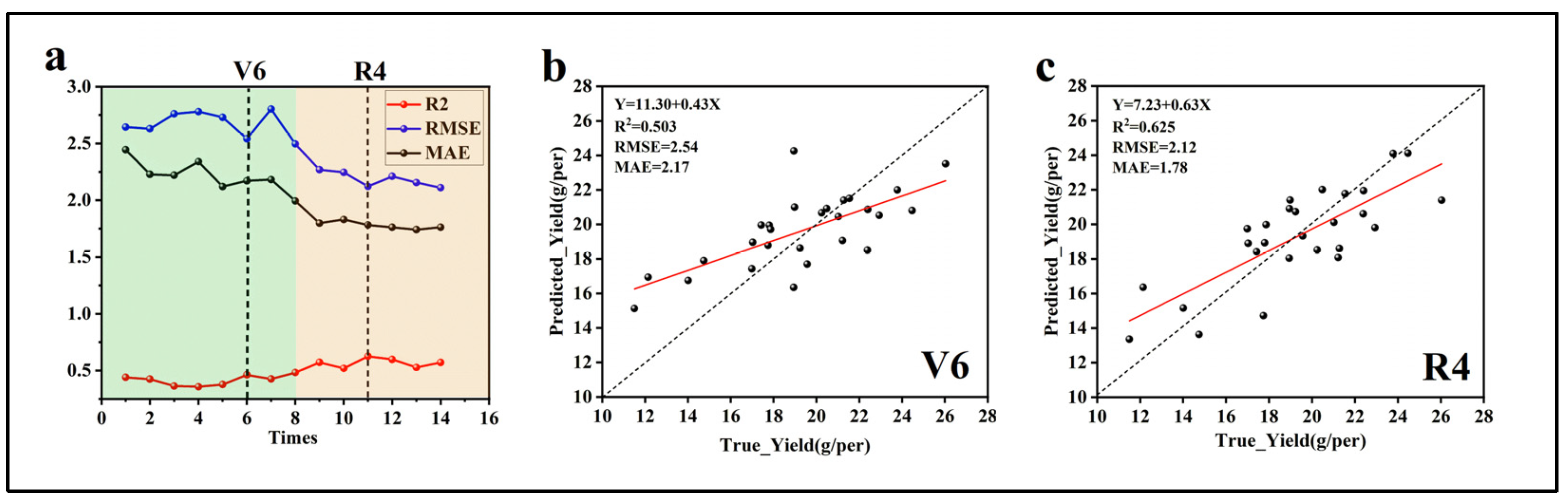
2.3. Establishment and Evaluation of the Prediction Model
2.4. Data Analysis Software
3. Experimental Results
3.1. Three-Dimensional Reconstruction Image Acquisition Parameters
3.1.1. Imaging Angle
3.1.2. Plant Rotation Speed
3.1.3. Number of Images Required for 3D Reconstruction
3.2. Point Cloud Preprocessing Results
3.2.1. Spatial Angle Transformation
3.2.2. Point Cloud Segmentation
3.2.3. Point Cloud Denoising
3.2.4. Point Cloud Scaling
3.3. Parameter Extraction
3.3.1. One-Dimensional Parameters
3.3.2. Two-Dimensional Parameters
3.3.3. Three-Dimensional Parameters
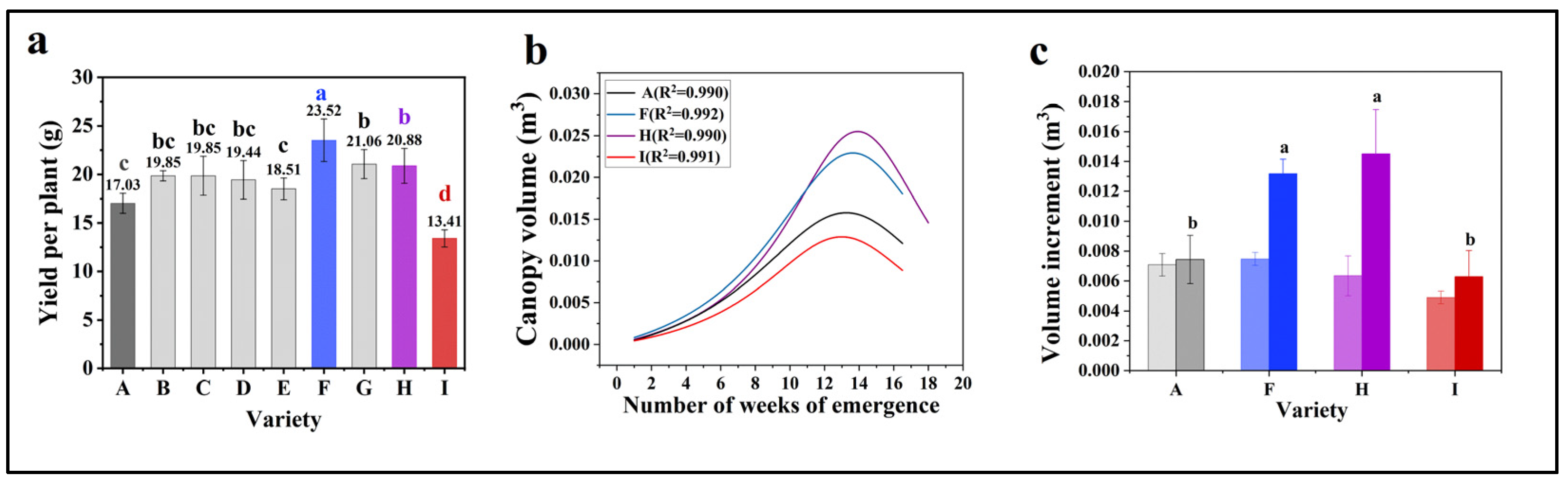
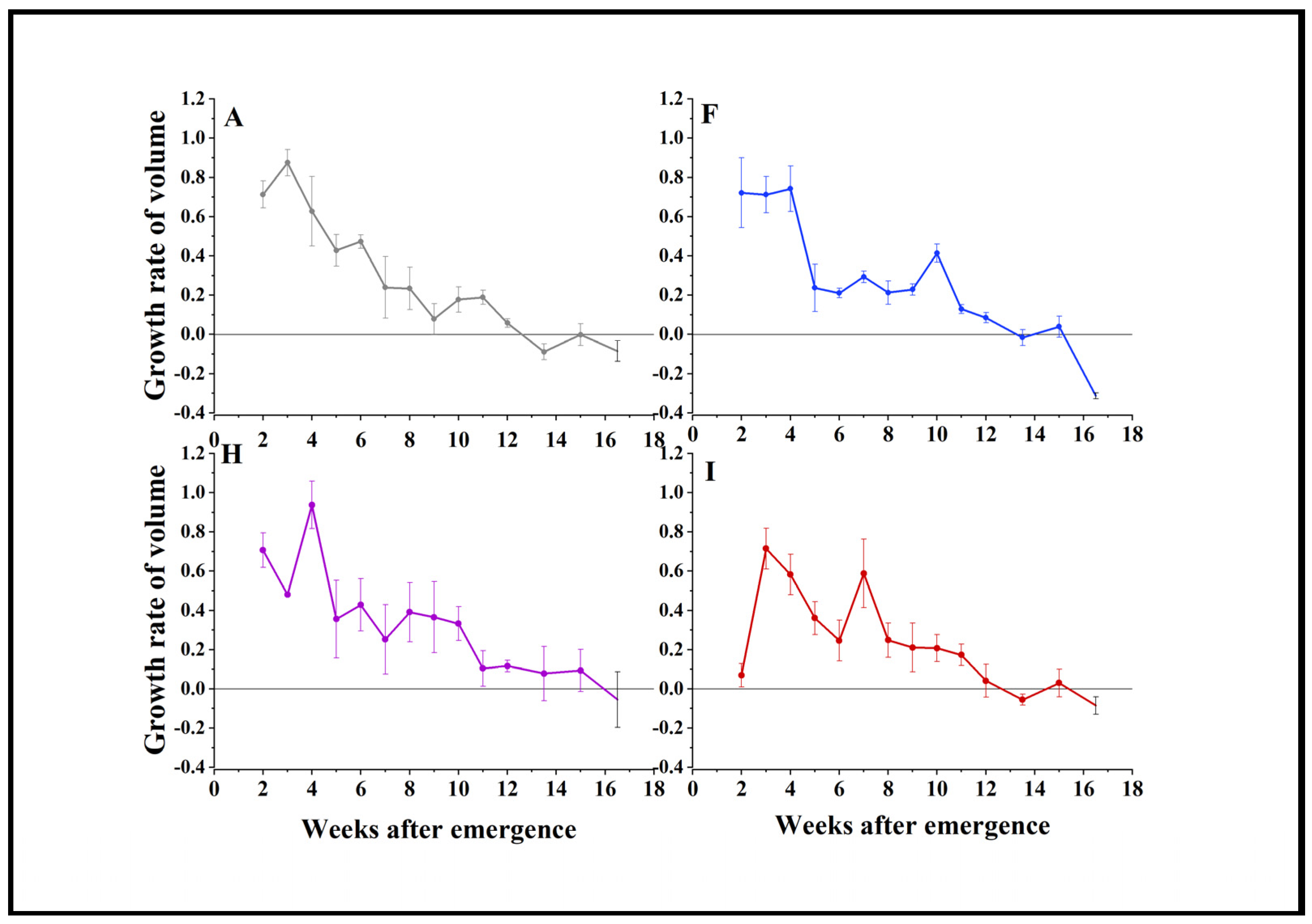
3.4. Soybean Yield Prediction
4. Discussion
5. Conclusions
Author Contributions
Funding
Data Availability Statement
Conflicts of Interest
References
- Skidmore, M.E.; Sims, K.M.; Gibbs, H.K. Agricultural intensification and childhood cancer in Brazil. Proc. Natl. Acad. Sci. USA 2023, 120, e2306003120. [Google Scholar] [CrossRef] [PubMed]
- Li, X.-F.; Wang, Z.-G.; Bao, X.-G.; Sun, J.-H.; Yang, S.-C.; Wang, P.; Wang, C.-B.; Wu, J.-P.; Liu, X.-R.; Tian, X.-L. Long-term increased grain yield and soil fertility from intercropping. Nat. Sustain. 2021, 4, 943–950. [Google Scholar] [CrossRef]
- Tsay, J.; Fukai, S.; Wilson, G. Effects of relative sowing time of soybean on growth and yield of cassava in cassava/soybean intercropping. Field Crops Res. 1988, 19, 227–239. [Google Scholar]
- Mbah, E.U.; Ogidi, E. Effect of soybean plant populations on yield and productivity of cassava and soybean grown in a cassava-based intercropping system. Trop. Subtrop. Agroecosyst. 2012, 15, 241–248. [Google Scholar]
- Buehring, N.; Reginelli, D.; Blaine, M. Long term wheat and soybean response to an intercropping system. In Proceedings of the Southern Conservation Tillage Conference, Raleigh, NC, USA, 16–17 July 1990; Citeseer: Princeton, NJ, USA, 1990; pp. 65–68. [Google Scholar]
- Li, L.; Sun, J.; Zhang, F.; Li, X.; Yang, S.; Rengel, Z. Wheat/maize or wheat/soybean strip intercropping: I. Yield advantage and interspecific interactions on nutrients. Field Crops Res. 2001, 71, 123–137. [Google Scholar]
- Li, L.; Sun, J.; Zhang, F.; Li, X.; Rengel, Z.; Yang, S. Wheat/maize or wheat/soybean strip intercropping: II. Recovery or compensation of maize and soybean after wheat harvesting. Field Crops Res. 2001, 71, 173–181. [Google Scholar]
- Chen, P.; Song, C.; Liu X-m Zhou, L.; Yang, H.; Zhang, X.; Zhou, Y.; Du, Q.; Pang, T.; Fu, Z.-D. Yield advantage and nitrogen fate in an additive maize-soybean relay intercropping system. Sci. Total Environ. 2019, 657, 987–999. [Google Scholar] [CrossRef]
- Wang, X.; Feng, Y.; Yu, L.; Shu, Y.; Tan, F.; Gou, Y.; Luo, S.; Yang, W.; Li, Z.; Wang, J. Sugarcane/soybean intercropping with reduced nitrogen input improves crop productivity and reduces carbon footprint in China. Sci. Total Environ. 2020, 719, 137517. [Google Scholar]
- Ghosh, P.; Tripathi, A.; Bandyopadhyay, K.; Manna, M. Assessment of nutrient competition and nutrient requirement in soybean/sorghum intercropping system. Eur. J. Agron. 2009, 31, 43–50. [Google Scholar]
- Egbe, O. Effects of plant density of intercropped soybean with tall sorghum on competitive ability of soybean and economic yield at Otobi, Benue State, Nigeria. J. Cereals Oilseeds 2010, 1, 1–10. [Google Scholar]
- Saudy, H.; El-Metwally, I. Weed management under different patterns of sunflower-soybean intercropping. J. Cent. Eur. Agric. 2009, 10, 41–51. [Google Scholar]
- Qin, C.; Li Y-h Li, D.; Zhang, X.; Kong, L.; Zhou, Y.; Lyu, X.; Ji, R.; Wei, X.; Cheng, Q. PH13 improves soybean shade traits and enhances yield for high-density planting at high latitudes. Nat. Commun. 2023, 14, 6813. [Google Scholar] [CrossRef] [PubMed]
- Zhu, Z.; Kleinn, C.; Nölke, N. Towards tree green crown volume: A methodological approach using terrestrial laser scanning. Remote Sens. 2020, 12, 1841. [Google Scholar] [CrossRef]
- Wang, J.; Zhang, Y.; Gu, R. Research status and prospects on plant canopy structure measurement using visual sensors based on three-dimensional reconstruction. Agriculture 2020, 10, 462. [Google Scholar] [CrossRef]
- Fahlgren, N.; Gehan, M.A.; Baxter, I. Lights, camera, action: High-throughput plant phenotyping is ready for a close-up. Curr. Opin. Plant Biol. 2015, 24, 93–99. [Google Scholar] [CrossRef]
- Liu, G.; Si, Y.; Feng, J. Research Progress on 3D Reconstruction Methods for Agricultural and Forestry Crops. Trans. Chin. Soc. Agric. Mach. 2014, 45, 38–46. [Google Scholar]
- Kaminuma, E.; Heida, N.; Tsumoto, Y.; Yamamoto, N.; Goto, N.; Okamoto, N.; Konagaya, A.; Matsui, M.; Toyoda, T. Automatic quantification of morphological traits via three-dimensional measurement of Arabidopsis. Plant J. 2004, 38, 358–365. [Google Scholar] [CrossRef]
- Alenya, G.; Dellen, B.; Foix, S.; Torras, C. Robotized plant probing: Leaf segmentation utilizing time-of-flight data. IEEE Robot. Autom. Mag. 2013, 20, 50–59. [Google Scholar] [CrossRef]
- Ivanov, N.; Boissard, P.; Chapron, M.; Andrieu, B. Computer stereo plotting for 3-D reconstruction of a maize canopy. Agric. For. Meteorol. 1995, 75, 85–102. [Google Scholar] [CrossRef]
- Biskup, B.; Scharr, H.; Schurr, U.; Rascher, U. A stereo imaging system for measuring structural parameters of plant canopies. Plant Cell Environ. 2007, 30, 1299–1308. [Google Scholar] [CrossRef]
- Wang, J.; Zhong, Y.; Dai, Y.; Birchfield, S.; Zhang, K.; Smolyanskiy, N.; Li, H. Deep two-view structure-from-motion revisited. In Proceedings of the IEEE/CVF conference on Computer Vision and Pattern Recognition, Nashville, TN, USA, 20–25 June 2021; pp. 8953–8962. [Google Scholar]
- Wu, D.; Yu, L.; Ye, J.; Zhai, R.; Duan, L.; Liu, L.; Wu, N.; Geng, Z.; Fu, J.; Huang, C. Panicle-3D: A low-cost 3D-modeling method for rice panicles based on deep learning, shape from silhouette, and supervoxel clustering. Crop J. 2022, 10, 1386–1398. [Google Scholar] [CrossRef]
- Thapa, S.; Zhu, F.; Walia, H.; Yu, H.; Ge, Y. A novel LiDAR-based instrument for high-throughput, 3D measurement of morphological traits in maize and sorghum. Sensors 2018, 18, 1187. [Google Scholar] [CrossRef] [PubMed]
- Li, M.; Shamshiri, R.R.; Schirrmann, M.; Weltzien, C. Impact of camera viewing angle for estimating leaf parameters of wheat plants from 3D point clouds. Agriculture 2021, 11, 563. [Google Scholar] [CrossRef]
- Li, Y.; Liu, J.; Zhang, B.; Wang, Y.; Yao, J.; Zhang, X.; Fan, B.; Li, X.; Hai, Y.; Fan, X. Three-dimensional reconstruction and phenotype measurement of maize seedlings based on multi-view image sequences. Front. Plant Sci. 2022, 13, 974339. [Google Scholar] [CrossRef]
- Maimaitijiang, M.; Sagan, V.; Sidike, P.; Hartling, S.; Esposito, F.; Fritschi, F.B. Soybean yield prediction from UAV using multimodal data fusion and deep learning. Remote Sens. Environ. 2020, 237, 111599. [Google Scholar] [CrossRef]
- Vatter, T.; Gracia-Romero, A.; Kefauver, S.C.; Nieto-Taladriz, M.T.; Aparicio, N.; Araus, J.L. Preharvest phenotypic prediction of grain quality and yield of durum wheat using multispectral imaging. Plant J. 2022, 109, 1507–1518. [Google Scholar] [CrossRef]
- Fei, S.; Hassan, M.A.; Xiao, Y.; Su, X.; Chen, Z.; Cheng, Q.; Duan, F.; Chen, R.; Ma, Y. UAV-based multi-sensor data fusion and machine learning algorithm for yield prediction in wheat. Precis. Agric. 2023, 24, 187–212. [Google Scholar] [CrossRef]
- Shen, Y.; Mercatoris, B.; Cao, Z.; Kwan, P.; Guo, L.; Yao, H.; Cheng, Q. Improving wheat yield prediction accuracy using LSTM-RF framework based on UAV thermal infrared and multispectral imagery. Agriculture 2022, 12, 892. [Google Scholar] [CrossRef]
- Nevavuori, P.; Narra, N.; Linna, P.; Lipping, T. Crop yield prediction using multitemporal UAV data and spatio-temporal deep learning models. Remote Sens. 2020, 12, 4000. [Google Scholar] [CrossRef]
- Revenga, J.C.; Trepekli, K.; Oehmcke, S.; Jensen, R.; Li, L.; Igel, C.; Gieseke, F.C.; Friborg, T. Above-ground biomass prediction for croplands at a sub-meter resolution using UAV–LiDAR and machine learning methods. Remote Sens. 2022, 14, 3912. [Google Scholar] [CrossRef]
- Wen, W.; Wu, S.; Lu, X.; Liu, X.; Gu, S.; Guo, X. Accurate and semantic 3D reconstruction of maize leaves. Comput. Electron. Agric. 2024, 217, 108566. [Google Scholar] [CrossRef]
- Rungyaem, K.; Sukvichai, K.; Phatrapornnant, T.; Kaewpunya, A.; Hasegawa, S. Comparison of 3D Rice Organs Point Cloud Classification Techniques. In Proceedings of the 2021 25th International Computer Science and Engineering Conference (ICSEC), Chiang Rai, Thailand, 18–20 November 2021; IEEE: New York, NY, USA, 2021; pp. 196–199. [Google Scholar]
- Gu, W.; Wen, W.; Wu, S.; Zheng, C.; Lu, X.; Chang, W.; Xiao, P.; Guo, X. 3D Reconstruction of Wheat Plants by Integrating Point Cloud Data and Virtual Design Optimization. Agriculture 2024, 14, 391. [Google Scholar] [CrossRef]
- Patel, A.K.; Park, E.-S.; Lee, H.; Priya, G.L.; Kim, H.; Joshi, R.; Arief, M.A.A.; Kim, M.S.; Baek, I.; Cho, B.-K. Deep Learning-Based Plant Organ Segmentation and Phenotyping of Sorghum Plants Using LiDAR Point Cloud. IEEE J. Sel. Top. Appl. Earth Obs. Remote Sens. 2023, 16, 8492–8507. [Google Scholar]
- Sun, Y.; Miao, L.; Zhao, Z.; Pan, T.; Wang, X.; Guo, Y.; Xin, D.; Chen, Q.; Zhu, R. An efficient and automated image preprocessing using semantic segmentation for improving the 3D reconstruction of soybean plants at the vegetative stage. Agronomy 2023, 13, 2388. [Google Scholar] [CrossRef]
- Zhu, R.; Sun, K.; Yan, Z.; Yan, X.; Yu, J.; Shi, J.; Hu, Z.; Jiang, H.; Xin, D.; Zhang, Z. Analysing the phenotype development of soybean plants using low-cost 3D reconstruction. Sci. Rep. 2020, 10, 7055. [Google Scholar]
- Fang, W.; Feng, H.; Yang, W.; Liu, Q. Rapid 3D Reconstruction Method for Wheat Plant Type Research in Phenotypic Detection. China Agric. Sci. Technol. Bulletin. 2016, 18, 95–101. [Google Scholar] [CrossRef]
- Ling, S.; Li, J.; Ding, L.; Wang, N. Multi-View Jujube Tree Trunks Stereo Reconstruction Based on UAV Remote Sensing Imaging Acquisition System. Appl. Sci. 2024, 14, 1364. [Google Scholar] [CrossRef]
- Jiang, Y.; Li, C.; Paterson, A.H.; Sun, S.; Xu, R.; Robertson, J. Quantitative analysis of cotton canopy size in field conditions using a consumer-grade RGB-D camera. Front. Plant Sci. 2018, 8, 2233. [Google Scholar]
- Andújar, D.; Escolà, A.; Rosell-Polo, J.R.; Ribeiro, A.; San Martín, C.; Fernández-Quintanilla, C.; Dorado, J. Using depth cameras for biomass estimation—A multi-angle approach. In Precision Agriculture’15; Wageningen Academic: Wageningen, The Netherlands, 2015; pp. 97–102. [Google Scholar]
- Liu, W.-G.; Jiang, T.; Zhou, X.-R.; Yang, W.-Y. Characteristics of expansins in soybean (Glycine max) internodes and responses to shade stress. Asian J. Crop Sci. 2011, 3, 26–34. [Google Scholar] [CrossRef]
- Javadnejad, F.; Slocum, R.K.; Gillins, D.T.; Olsen, M.J.; Parrish, C.E. Dense point cloud quality factor as proxy for accuracy assessment of image-based 3D reconstruction. J. Surv. Eng. 2021, 147, 04020021. [Google Scholar] [CrossRef]
- Ma, X.; Zhu, K.; Guan, H.; Feng, J.; Yu, S.; Liu, G. Calculation method for phenotypic traits based on the 3D reconstruction of maize canopies. Sensors 2019, 19, 1201. [Google Scholar] [CrossRef] [PubMed]
- Zhu, C.; Miao, T.; Xu, T.; Yang, T.; Li, N. Stem-leaf segmentation and phenotypic trait extraction of maize shoots from three-dimensional point cloud. arXiv 2020, arXiv:200903108. [Google Scholar]
- Ma, X.; Zhu, K.; Guan, H.; Feng, J.; Yu, S.; Liu, G. High-throughput phenotyping analysis of potted soybean plants using colorized depth images based on a proximal platform. Remote Sens. 2019, 11, 1085. [Google Scholar] [CrossRef]
- Wang, F.; Ma, X.; Liu, M.; Wei, B. Three-dimensional reconstruction of soybean canopy based on multivision technology for calculation of phenotypic traits. Agronomy 2022, 12, 692. [Google Scholar] [CrossRef]
- Xu, W.; Feng Zh Su, Z.; Xu, H.; Jiao Yo Deng, O. An Automatic Extraction Algorithm for Individual Tree Canopy Projection Area and Canopy Volume Based on 3D Laser Point Cloud Data. Spectrosc. Spectr. Anal. 2014, 34, 465–471. [Google Scholar]
- Li Xi Tang, L.; Huang, H.; Chen Ch He, J. A Method for Estimating Individual Tree 3D Green Volume Based on Point Cloud Data. Remote Sens. Technol. Appl. 2022, 37, 1119–1127. [Google Scholar]
- Li, Q.; Gao, X.; Fei, X.; Zhang, H.; Wang, J.; Cui, Y.; Li, B. Constructing Tree Canopy 3D Models Using the Alpha-shape Algorithm. Surv. Mapp. Bulletin. 2018, 91–95. [Google Scholar] [CrossRef]
- Lee, B.; Di Girolamo, L.; Zhao, G.; Zhan, Y. Three-Dimensional Cloud Volume Reconstruction from the Multi-angle Imaging SpectroRadiometer. Remote Sens. 2018, 10, 1858. [Google Scholar] [CrossRef]

| Rotation Speed (rpm) | IOU | PA | Recall |
|---|---|---|---|
| 0.8 | 0.97 | 0.98 | 0.97 |
| 1.0 | 0.97 | 0.98 | 0.97 |
| 1.2 | 0.97 | 0.97 | 0.97 |
| 1.4 | 0.95 | 0.95 | 0.95 |
| Dimensions | Methods | Image Indexes |
|---|---|---|
| One-dimensional | - | Plant height, plant length, plant width, centroid height, minimum bounding box length, minimum bounding box width, minimum bounding box height, centroid height ratio. |
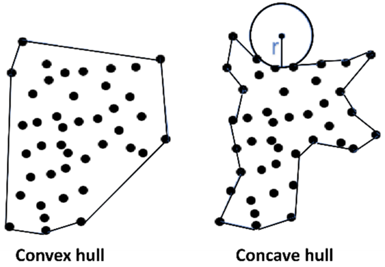
| Two-dimensional | Convex hull | Top projection convex hull area, side projection convex hull area. |
| Concave hull | Top projection concave hull area, side projection concave hull area. | |
| Three-dimensional | Convex hull | Convex hull volume, convex hull surface area, layered convex hull surface area, layered convex hull volume. |
| Voxel | Voxel volume, voxel surface area, voxel surface area ratio (top/bottom), minimum bounding box volume, minimum bounding box surface area. | |
| α-shape | α-shape volume, α-shape surface area, canopy upper-to-lower volume ratio. |
Disclaimer/Publisher’s Note: The statements, opinions and data contained in all publications are solely those of the individual author(s) and contributor(s) and not of MDPI and/or the editor(s). MDPI and/or the editor(s) disclaim responsibility for any injury to people or property resulting from any ideas, methods, instructions or products referred to in the content. |
© 2025 by the authors. Licensee MDPI, Basel, Switzerland. This article is an open access article distributed under the terms and conditions of the Creative Commons Attribution (CC BY) license (https://creativecommons.org/licenses/by/4.0/).
Share and Cite
Li, X.; Chen, M.; He, S.; Xu, X.; Shao, P.; Su, Y.; He, L.; Qiao, J.; Xu, M.; Zhao, Y.; et al. Optimization of the Canopy Three-Dimensional Reconstruction Method for Intercropped Soybeans and Early Yield Prediction. Agriculture 2025, 15, 729. https://doi.org/10.3390/agriculture15070729
Li X, Chen M, He S, Xu X, Shao P, Su Y, He L, Qiao J, Xu M, Zhao Y, et al. Optimization of the Canopy Three-Dimensional Reconstruction Method for Intercropped Soybeans and Early Yield Prediction. Agriculture. 2025; 15(7):729. https://doi.org/10.3390/agriculture15070729
Chicago/Turabian StyleLi, Xiuni, Menggen Chen, Shuyuan He, Xiangyao Xu, Panxia Shao, Yahan Su, Lingxiao He, Jia Qiao, Mei Xu, Yao Zhao, and et al. 2025. "Optimization of the Canopy Three-Dimensional Reconstruction Method for Intercropped Soybeans and Early Yield Prediction" Agriculture 15, no. 7: 729. https://doi.org/10.3390/agriculture15070729
APA StyleLi, X., Chen, M., He, S., Xu, X., Shao, P., Su, Y., He, L., Qiao, J., Xu, M., Zhao, Y., Yang, W., Maes, W. H., & Liu, W. (2025). Optimization of the Canopy Three-Dimensional Reconstruction Method for Intercropped Soybeans and Early Yield Prediction. Agriculture, 15(7), 729. https://doi.org/10.3390/agriculture15070729