1. Introduction
Drought poses an enormous threat to crop production. Altered precipitation patterns are expected to increase the frequency and severity of drought in coming years [
1]. Soybean is the most widely grown legume crop on Earth, and water availability is a major determinant of its yield [
2]. Improving soybean’s drought resilience is important for global food security [
3]. Leaf wilting is a visually obvious symptom of drought stress in soybeans, resulting from reduced turgor pressure as leaf water loss via evapotranspiration exceeds water resupply into the leaf. Despite multiple methodologies for quantifying drought stress with instrumentation, visual scoring of leaf wilt remains the dominant method for plant breeders and agronomists due to the speed with which it can be conducted. Soybean researchers often use visual scores of leaf wilting to assess a particular genotype’s potential drought tolerance and select the best lines to advance towards a new variety. The method has significant disadvantages as well, including significant variations between observers and the inability of human observers to evaluate all plots or genotypes at the same moment in time [
4,
5,
6]. These scores are also slow and labor-intensive to collect, normally assigned by walking through the crop fields and manually inspecting the level of wilting on the leaves, and assigning a value along a predetermined scale to indicate the degree of stress [
7,
8]. In the field of precision agriculture, machine learning (ML) and DL techniques have been widely used to automate many tedious and repetitive tasks on the field [
9,
10]. Low-cost imaging systems equipped with cloud access or local compute capabilities can be used to evaluate drought stress under real-world field conditions [
11].
In our study, we have explored a DL technique called multiple instance learning (MIL) [
12,
13,
14] to classify leaf wilting in soybean plants. MIL is a supervised learning technique that is used to find key instances among a collection of instances, also termed as a bag. Other than modeling ambiguity in datasets, it also provides a way to leverage weak labels on images, where a single label is provided for the entire bag instead of individual instances [
15,
16]. The MIL approach treats the input dataset as a collection of bags, each bag consisting of a collection of instances in the form of patches. A bag is assigned a positive label if it contains at least one instance belonging to the relevant class. If no such instances appear, the bag is labeled negative. Apart from predicting a bag/classification label, such a model is also able to highlight regions of interest (ROIs) in the image that were responsible for triggering a particular label. Dietrich et al. [
13] first introduced the term MIL in an attempt to solve the drug activation problem. They used MIL to find specific molecular conformations among all observed low-energy shapes that contributed towards making a drug active. Maron and Ratan [
14] used MIL in image classification of natural scenes. An image was considered a bag and each bag had subimages termed as instances. In the field of agriculture, MIL has been used for automatic wheat disease diagnosis [
17], pest classification in citrus plants [
18], and automatic counting of cotton flower from aerial imagery [
19], among others. MIL also finds use in a wide variety of applications, from object tracking [
20,
21] to medical data analysis [
22,
23,
24,
25]. Ilse, Tomzack, and Welling [
26] formulated the MIL problem as a Bernoulli distribution of the bag label. They provide a three-step procedure for modeling the bag probability to classify medical images into cancerous and non-cancerous categories. Additionally, they introduce the attention mechanism to their model to find key instances that highlight malignant cells in the images.
Our study focuses on the detection of drought stress in soybean plants by analyzing leaf wilt from images of the crop. This image-based wilt detection has the potential to be a valuable tool for characterizing the drought tolerance in different soybean varieties, a crucial factor given the strong impact of water availability on crop yield. We have implemented a deep MIL multi-class classification model for this task. The following are some of the key contributions made in our study:
We introduce a labeled dataset of soybean field images with each image assigned a value between 0 and 1 by expert annotators.
We introduce a deep MIL multi-class classification model by converting the MIL approach, generally well suited for binary classification, to handle multiple classes.
Along with providing classification scores, we explore the use of our model to provide interpretability by generating heat maps that highlight ROIs in the images with the intent to allow researchers to pinpoint relevant areas of drought stress in the field.
We demonstrate that our MIL model achieves classification accuracy on par with state-of-the-art classification models like DenseNet 121 [
27] and ViT [
28]. This model is also able to achieve high one-off accuracy, an important performance metric for our dataset as we will see later. Unlike larger models like ViT, the smaller architecture of our MIL model also ensures faster prediction time which is essential for real world deployment on IoT/edge devices.
Lastly, we are able to show the benefit of utilizing our deep learning model over expert human scorers, and that relying solely on expert decisions is often not the most accurate, efficient, effective, and reproducible approach.
The rest of the paper is organized as follows. In
Section 2, we introduce our dataset of soybean field images, each assigned with a wilt label by expert annotators. In
Section 3, we provide details on our MIL model along with it is mathematical formulation and compare model architecture and training parameters with our baseline models. We also provide our experimental details in this section. In
Section 4, we report on classification performance of both our binary and multi-class MIL models and compare with the baseline models of DenseNet 121 and ViT. We also include results of our study of human variability in annotations and effect of varying patch size and patch overlap ratio on the different performance metrics such as accuracy, one-off accuracy, root mean square error (RMSE), and mean absolute error (MAE).
2. Dataset
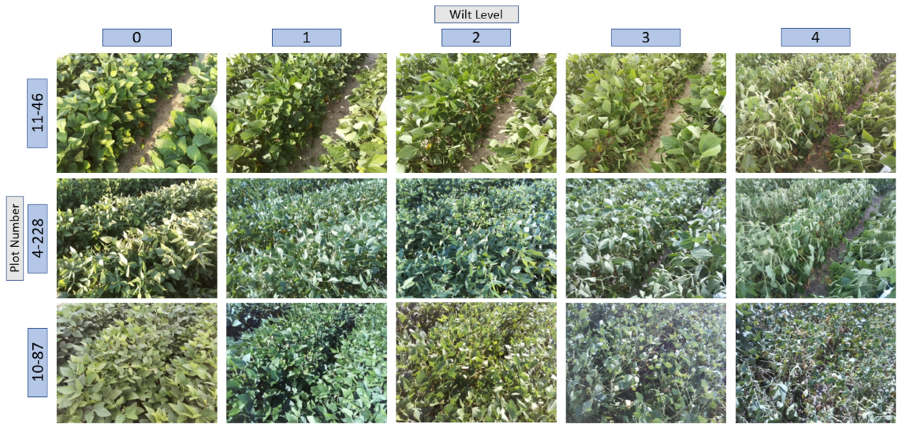
The dataset produced in collaboration with the Crop and Soil Science Department of North Carolina State University and the United States Department of Agricultural Research Service (USDA-ARS) comprises 1788 images. Images were taken in 16 plots within a field at Sandhills Research Station in Jackson Springs, NC, USA. Cameras were mounted 1.52 m above the soybean canopy at an angle of 45 degrees and were programmed to capture an image of the plot every 15 min from sunrise to sunset over a period of 8 weeks in August and September of 2020. Half of the plots were irrigated throughout this period, and half of the plots were rain-fed only from 8 August through 15 September. The images represent soybean plants having different levels of wilting, each image being assigned a value between 0 and 5 by expert annotators, where 0 represents leaves with no wilting, 1 represents leaflets folding inward at secondary pulvinus with no turgor loss in leaflets or petioles, 2 represents slight leaflet or petiole turgor loss in upper canopy, 3 represents moderate turgor loss in upper canopy, 4 represents severe turgor loss throughout upper canopy and some turgor loss in lower canopy, and 5 represents severe turgor loss throughout canopy. For ease of analysis and due to the presence of fewer images in class 5, 4 and 5 were combined into a single class 4.
Figure 1 shows some sample images from this dataset.
Table 1 shows the distribution of different classes and plot numbers in the dataset. Most plot numbers exhibited an unequal distribution of instances, with some plots missing instances in certain classes. The plot with the most balanced class distribution was 11–46, which was selected as a holdout test set for our experiments.
3. Materials and Methods
This section describes the models used for our prediction task and the computational experiments that were performed. Even though the inference task could be set up as a classification problem, we consider it more appropriate to pose it as a regression task since the ordering of the class labels does matter. That is, given a true class label of 0, it is worse to label something as 3 than it is to label it as 1. This motivates our use of metrics such as standard accuracy and one-off accuracy (i.e., predicted labels are considered correct if they are within 1 value of the true label).
3.1. Baseline Model
Different methods were explored in our attempt to create a baseline for the classification. Deep learning methods outperformed methods that used handcrafted features with traditional machine learning. As one of our baselines we included the popular image classification model, DenseNet121 [
27]. It is a type of deep convolutional neural network that belongs to the DenseNet family of models. Each layer is connected to every other layer in a feed-forward manner. This means that the output of each layer is fed into all subsequent layers. DenseNet-121 requires fewer parameters compared to traditional networks like VGG or ResNet, as its dense connectivity promotes feature reuse. This leads to better performance, faster convergence, and reduced risk of vanishing gradients. As our second baseline we chose a ViT, the current state of the art in image classification tasks, which is also equipped with a self-attention mechanism [
28]. A ViT is a transformer like architecture that handles vision processing tasks. It divides an input image into smaller patches (e.g., 16 × 16 or 32 × 32 pixels) and treats each patch as a “token”. Each patch is then flattened into a vector and passed through the transformer layers, where the self-attention mechanism learns relationships between patches, regardless of their spatial locations. Positional embeddings are added to the input vectors, providing information about each patch’s position in the image. Vision Transformers use the same transformer encoder architecture as in NLP, with multiple layers of self-attention and feed-forward networks to capture global context and long-range dependencies. When trained on large datasets like ImageNet [
29] or JFT-300M [
30], ViTs can outperform CNNs, achieving state-of-the-art performance in various vision tasks. A comparison of the model architectures and performance is presented in
Section 3.3.
3.2. Multiple Instance Learning (MIL) Model
Drawing inspiration from [
26], we modified their binary classification model to a multi-class classification approach. Our MIL model is able to classify images taken from soybean fields into five different wilting levels as well as find ROIs in the images in the form of heat maps. Previously reported work on the same dataset achieved a classification accuracy of 88% using DenseNet 121 [
11]. In order to mimic real world scenarios, we have used holdout sets to test our model on data entirely unseen during training. We show that, apart from achieving comparable accuracy to DenseNet 121 on the holdout set, our MIL model can also introduce interpretability and help researchers identify relevant areas of drought stress in the images.
In their work, Ilse, Tomczak, and Welling [
26] formulate the bag probability as a Bernoulli distribution, meaning their model can only classify images into two categories. The MIL approach in general is well suited for 0/1, yes or no solutions, where the problem is looking for a presence or absence of a category, for example if malignant cells are present or absent in an image and where such instances of malignancy occur. One way of making such a model suitable for multi-class classification is to convert it to a regression problem instead of classification. To implement such a model, we removed the concept of a positive and a negative bag and instead considered bags belonging to five separate classes corresponding to the five levels of wilting.
Ilse, Tomczak, and Welling proposed a bag of instances as input to their model. Proceeding along the same line, we represent an image X as a bag of instances given by , where is a collection of K patches all having the same dimensions. It is assumed that individual patch labels exists but are unknown or inaccessible during training. Instead, we assign a label Y to the entire bag/image, with These assigned labels are discrete in nature, similar to labels in classification problems. However, we assume that these labels are derived from a continuous range in order to formulate our regression-based model.
Following the general three-step strategy in [
26] for classifying a bag of instances in a binary classification problem, we modify it to a multi-class problem as follows:
A transformation function converts each input instance to a low dimensional embedding , where M is the dimension of the embedding and is a neural network made up of a combination of convolutional and fully connected layers with parameters .
A symmetric permutation invariant function
is applied to the transformed instances
to generate an aggregated score/bag representation
z. This step is called MIL pooling. Three types of popular pooling methods were explored:
and
with
and
.
A function transforms the aggregated instance scores z to generate a bag score . is a neural network with parameters .
The training is performed by minimizing the mean square error (MSE) loss between the generated bag scores and the corresponding ground truth values. That is,
The authors in [
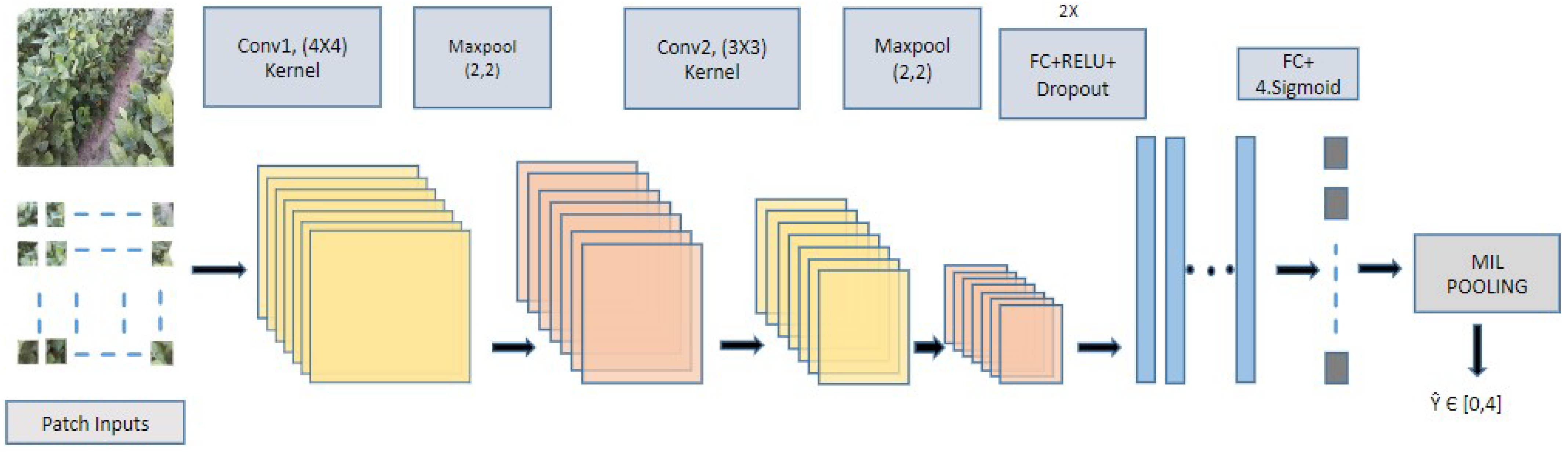
26] made use of the attention pooling to propose a novel Deep-Attention-based MIL. However, in our experiments, the more standard mean and max pooling outperformed their attention-based counterparts. This may be due to the small amount of data available for training. Our experiments make use of an instance-based MIL for which
is a neural network that returns a scalar value in the range
, we use either mean or max pooling, and
is set to be the identify function. The model architecture of our instance-based MIL is shown in
Figure 2.
An advantage of using a multiple instance learning model over direct regression models is its ability to generate attention maps. The instance score
that each patch receives is a measure of its contribution in the classification of the entire image. The attention maps are generated by multiplying the patches with their corresponding scores and stitching them back together to generate the whole image,
. The resulting attention maps
I thus highlight regions in the image that belong to a particular class and segments out all other areas. Example attention maps are shown in
Section 4.1 for our binary classification approach. For our multi-class classification approach, we have included heat maps instead of attention maps. The heat maps were generated by extracting the attention scores from the model, performing bilinear interpolation on them, and then overlaying the resulting heat maps on the original images. These heat maps can be used to study areas in the image that the model considers important in contributing to the predicted wilting level.
3.3. Implementation Details
In
Table 2, we show a comparison of our MIL multi-class classification model against the baseline models DenseNet 121 and a ViT. Here,
K stands for number of patches generated per image having dimensions
. Our images are of size
. Patch size for the ViT and the MIL model are
and
, respectively. In our experiments,
p was fixed at 16, which is consistent with the patch size selected in prior studies with ViTs, while we have varied patch size
for the MIL model to study its effect on classification performance.
We perform hyperparameter tuning to obtain optimal values for all our models. Training was performed over 100 epochs and data augmentation was performed on the train set using transformations like rotate, horizontal flip, sheer, zoom, and brightness adjustment. This was primarily performed to handle a small dataset and the presence of class imbalance in the dataset. For our MIL model, we used an ADAM optimizer [
32], learning rate (LR)
,
,
, and weight decay
. Following the protocol in [
26], we select a batch size = 1 corresponding to 1 bag and 10-fold cross validation for training. The DenseNet 121 was pre-trained on ImageNet 1k and finetuned on our dataset. Images were downsized to
, which is the size of the input for the pre-trained model used. Stochastic gradient descent (SGD) with Nesterov momentum [
33] was used for training with an exponential decay LR scheduler with LR and weight decay
, LR decay steps = 50,000, momentum
, and batch size
. Similarly for the ViT, pre-training was done on ImageNet 21k and then finetuned on our dataset. An ADAM optimizer with LR
was used with batch size of 32. All experiments were run on an Ubuntu workstation with an NVIDIA GeForce GTX 1080 Ti GPU.
Before being fed to the model, images were divided into patches of the same dimensions. Since the patches (and not the whole image) are fed to the model as input, the size and the number of patches in each bag is expected to affect performance of the model. Thus, a batch had one image in the form of K patches. The value of K varied based on the patch size and overlap ratio. We considered patch sizes equal to , , , , , and ; and overlap ratios of 0, 0.25, and 0.4. These values were varied to study their impact on performance.
Images belonging to plot number 11–46 were set aside as our test dataset. We have used confusion matrices and different metrics, namely accuracy, one-off accuracy, precision, F1 score, RMSE, and MAE to quantify the performance of our models. The one-off accuracy is an important metric in our analysis, as it demonstrated the difficulty of classifying the dataset into each individual class separately but showed that most incorrect classifications by the model occurred between adjacent classes. When reporting performance, we executed multiple runs of our experiments and reported the means and variances for all our metrics.
4. Results
We first explored the binary classification approach proposed in [
26] in
Section 4.1. Since this approach is suitable only for binary classification, we formulated our problem accordingly. One class or a combination of two classes were selected to represent a positive or a negative bag. Test results were reported on two MIL models and DenseNet121. Multi-class performance is reported in
Section 4.2. We further analyzed the effect of patch size and overlap ratio on the MIL approach in
Section 4.3.
Keeping in mind the complexity present in our dataset, we also wanted to quantify the amount of human variability present in labeling the images. This analysis gave us an insight into the difficulty in consistently determining a correct wilting level even for expert annotators. Images belonging to the holdout test set 11–46 were selected and sent to the experts for re-annotation with their IDs changed. Confusion matrices were computed by considering the original set of annotations as ground truth and the new set as predictions. We compared the results of the re-annotation to the performance of our MIL model in
Section 4.4.
4.1. MIL Binary Classification
Table 3 shows the results of binary classification with images from a subset of classes representing positive instances and images from other classes denoting the negative instances. The accuracy obtained is an indicator of the difficulty in classifying the different bag combinations. Accuracy was highest with class 4 as positive and class 0 as negative bags or vice versa. The accuracy showed a considerable decrease when adjacent classes were treated as positive and negative bags or even when a combination of classes were considered as a single bag. As expected, this showed that images belonging to adjacent wilting levels were more difficult to classify. The instance-based MIL with mean pooling outperformed the max pooling model, the attention-based MIL pooling model [
26], and showed results comparable to the baseline.
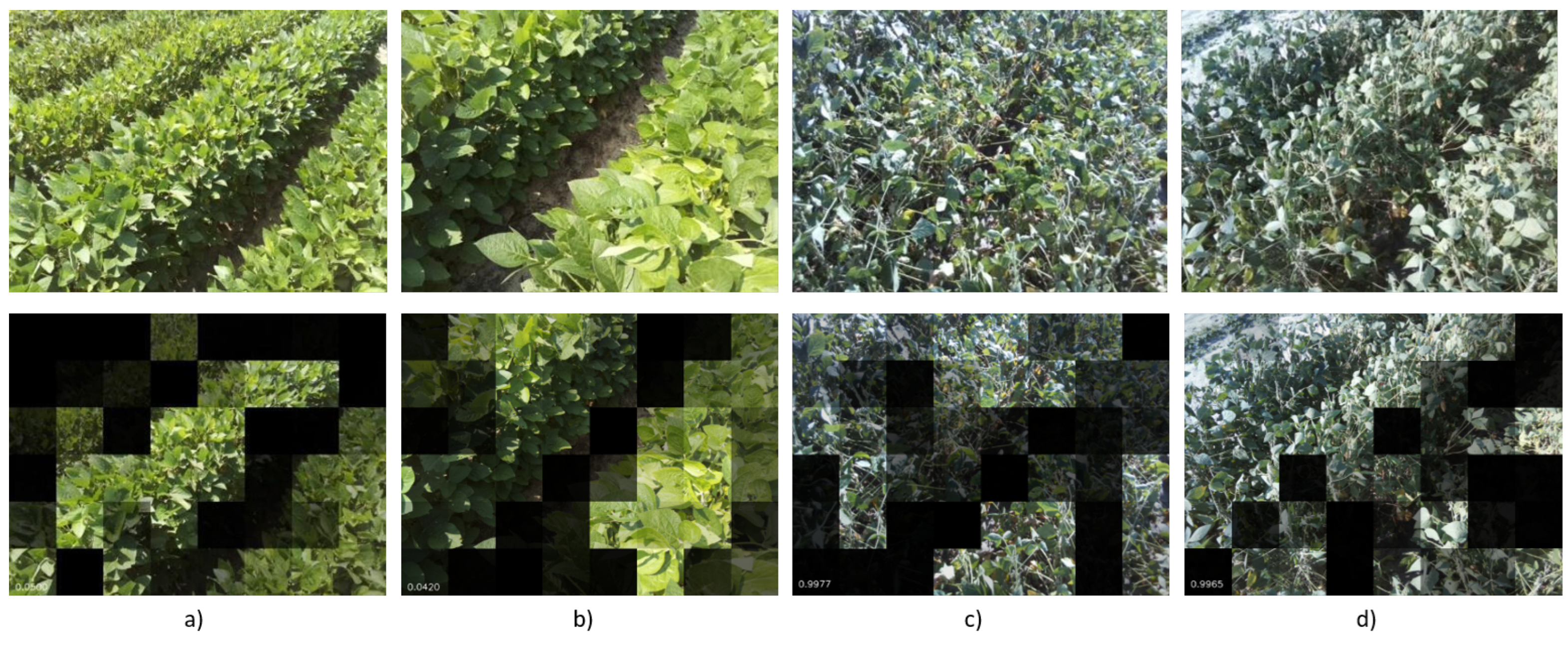
Some examples of attention maps of the soybean images generated by the model are shown in
Figure 3. The attention maps indicate the ROIs in the image that were responsible for the classification by the model. Regions in the image that contribute to a particular class get highlighted while those that did not make any contributions get a low impact score by the model, and hence, get blacked out. The attention maps are a good way of interpreting the decisions made by the model. They also segment out any areas in the field that are not relevant for the classification, including regions that do not contain any soybean plant (e.g., patches or columns of field appearing in between the plantations). The model also places less importance on patches that appear out of perspective in the images; for example, a leaf may appear too small or too large inside a patch.
4.2. MIL Multi-Class Classification
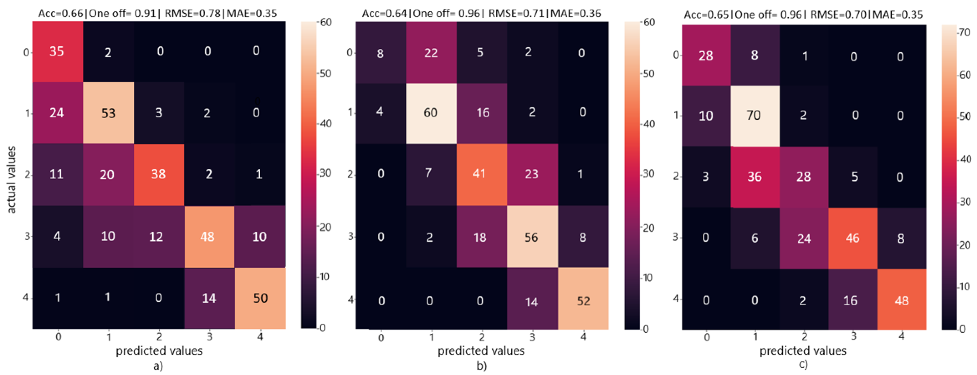
Confusion matrices (
Figure 4) were generated to study the performance of our MIL model on multi-class classification and compare them to the baseline models of DenseNet and ViT.
Table 4 shows a detailed result on different performance metrics for each of the three models. For our MIL model, performances reported correspond to a patch size of 80 × 120. We report on accuracy, one-off accuracy, precision, and F1 score per class as well as with all classes combined. We also report on combined RMSE, MAE, and speed of predictions made by each model. DenseNet outperformed the other two models in terms of overall accuracy by a small margin. Overall accuracy of all three models was limited due to the complexity of the dataset, particularly the similarity between adjacent classes. However, both our MIL model as well as the ViT outperformed the DenseNet in one-off accuracy, which is an important metric in our analysis. All three models performed significantly better in one-off accuracy compared to classification accuracy. This gave us an insight into the difficulty in classifying adjacent wilting rates but the relative ease in classifying wilting levels separated by more than one class. In terms of classification performance per class, it is interesting to note the significant difference in results for each model. Our MIL model outperforms the DenseNet in four out of five classes, and the ViT in three out of five classes. However, because of it is significant low classification accuracy for class 0, it achieves the lowest overall classification accuracy out of the three models. A considerable difference in architecture of the three models could lead to differences in learnt features. This coupled with the complexity present in the dataset could explain the wide class wise variability in classification performance. Our MIL model, despite having a smaller architecture than the baselines, was second fastest in prediction accuracy speed. The DenseNet 121 had the smallest number of trainable parameters because of it is small input size (224 × 224) and no input patches used for training. As a result, it achieved the highest prediction speed (0.56 s per image). Our MIL model, which was trained on patches of images of size 80 × 120 and a patch overlap of 0.25 (42 patches per image), achieved a slightly slower prediction speed of 0.61 s. The ViT model, which had the most architectural complexity and patches of size 16 × 16, had the slowest prediction speed.
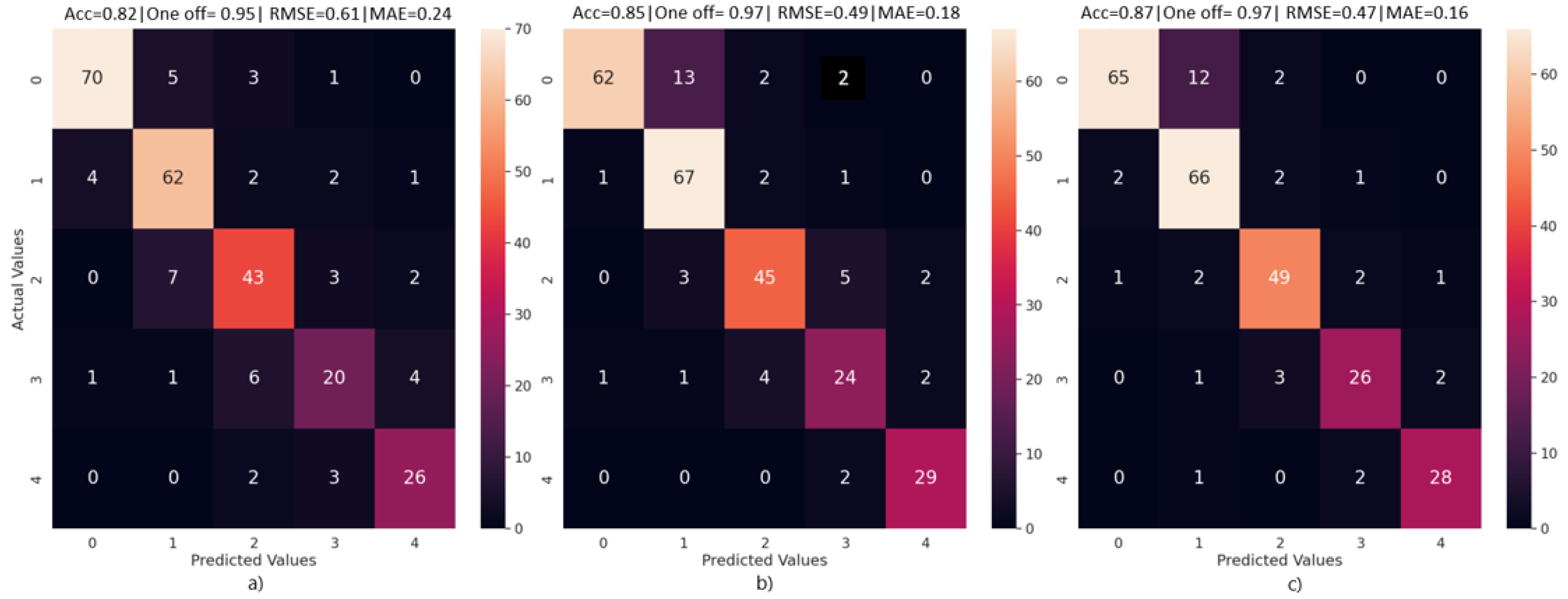
Figure 5 and
Table 5 show results of multi-class classification when a subset of images is randomly selected as the test set. In total, 15% of the dataset is randomly selected from each class and set aside as the test set. This resulted in 79, 71, 55, 32, and 31 instances of class 0, 1, 2, 3, and 4, respectively, in the test set. The train set was then subjected to data augmentation, as discussed in
Section 3. Comparing the results from the two multi-class classification experiments, we see that all three models for the randomly selected test subset case perform significantly better than the models which had holdout test images set aside during training. In
Table 5, it is observed that a combined accuracy of 0.85, 0.82, and 0.87 is obtained for the three models, whereas for the holdout test set scenario, these values are 0.64, 0.66, and 0.65, respectively, as seen in
Table 4. This is because the holdout method minimizes model bias. By having a select set of images from a specific plot set aside during model training, it ensures that during test time, the model produces realistic and not overly optimistic results on a new sample set, which was unseen during training.
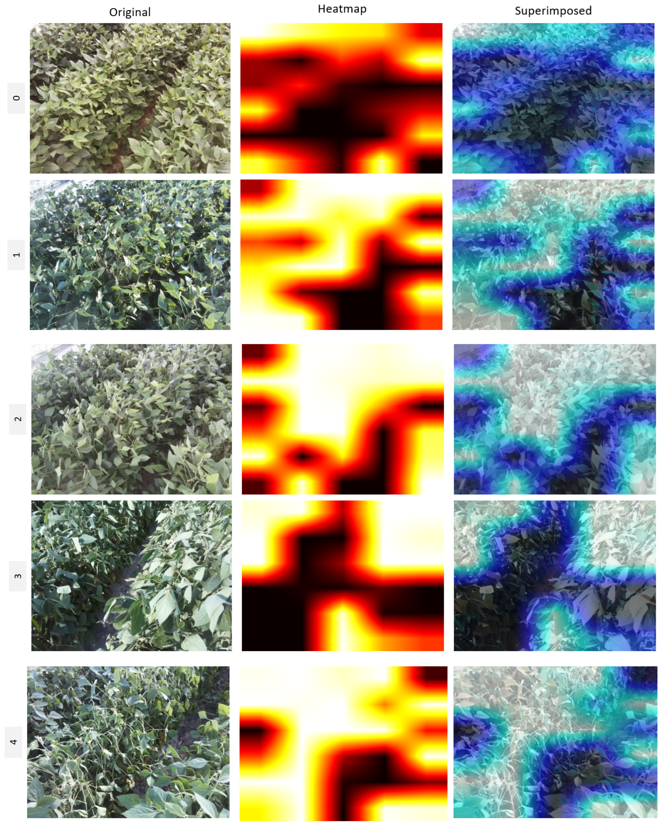
Figure 6 illustrates heat maps generated using the attention scores received by the patches in our MIL multi-class classification model for the holdout test set. These heat maps were created by extracting attention scores from the model, applying bilinear interpolation to the attention scores, and then overlaying the heat maps onto the original images. Like the attention maps shown in
Section 4.1, these heat maps highlight which areas of the image influenced the classification and which did not. It is evident that gaps between leaf columns and regions where leaves appear disproportionate receive less attention, as indicated by the blue regions on the superimposed images.
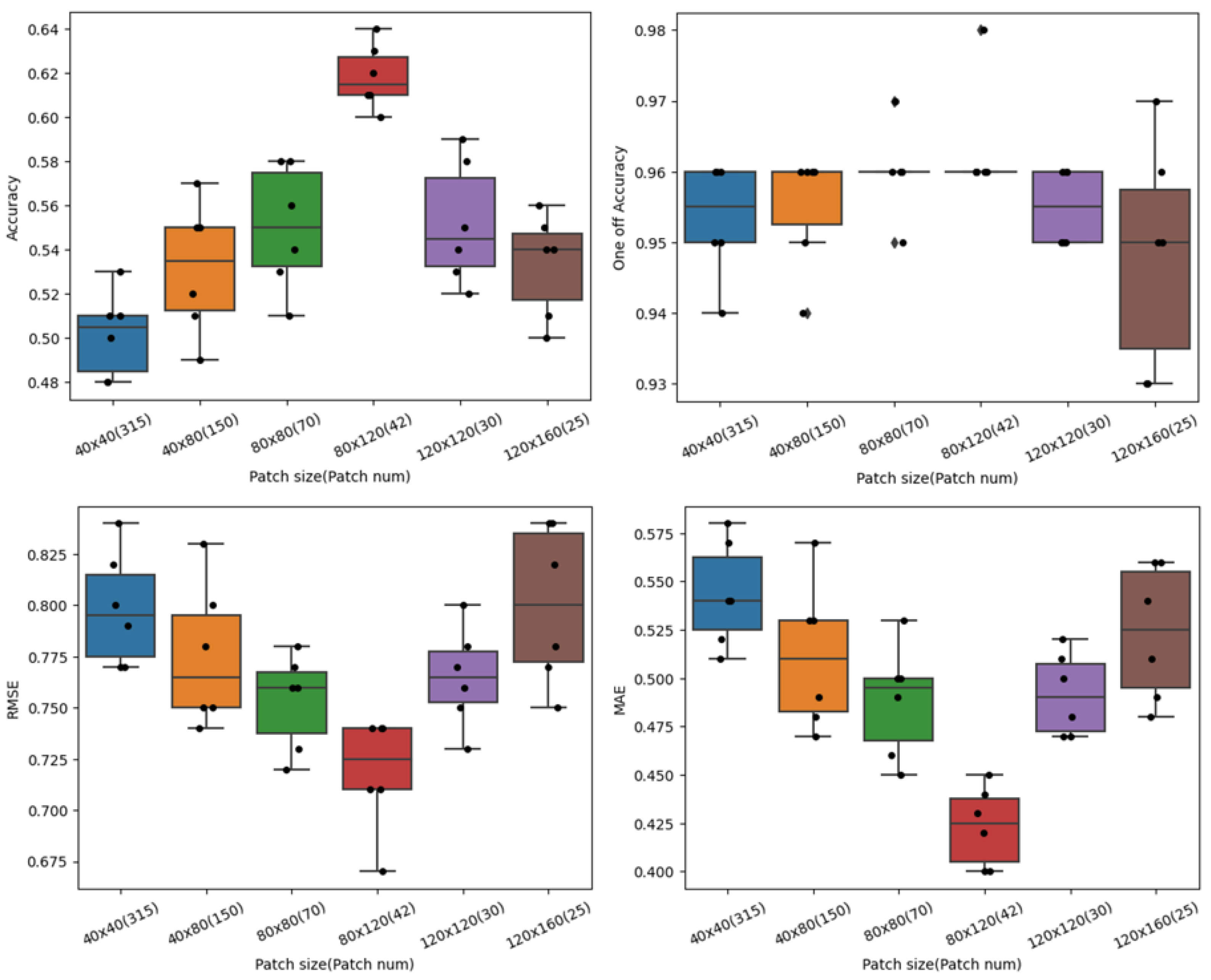
4.3. Patch Size vs. Patch Overlap Ratio
We also wanted to study how the number of patches present in a bag affected performance of the model. The number of patches an image is divided into and fed as input to the model depend on the patch size (
) and the overlap between the patches. Our experiments included an overlap of 0, 0.25, and 0.4 and patch sizes of 40 × 40, 40 × 80, 80 × 80, 80 × 120, 120 × 120, and 120 × 160. The results are shown in
Table 6. An overlap of 0.25 gave the best results for the majority of the patch sizes considered.
Figure 7 shows performance plots of the MIL model for varying patch sizes and an overlap of 25%. The plots show how the four different performance metrics of the model change with patch size. Multiple re-runs of the experiments were performed to report on a mean, and their standard deviation are shown in the plots. From the experiments, it was observed that there was considerable variance in performance when patch size was changed. The best results were obtained with a patch size of 80 × 120 and 42 patches in a bag. For all the other sizes, there was a significant decrease in performance as well as more variations in between experiment reruns.
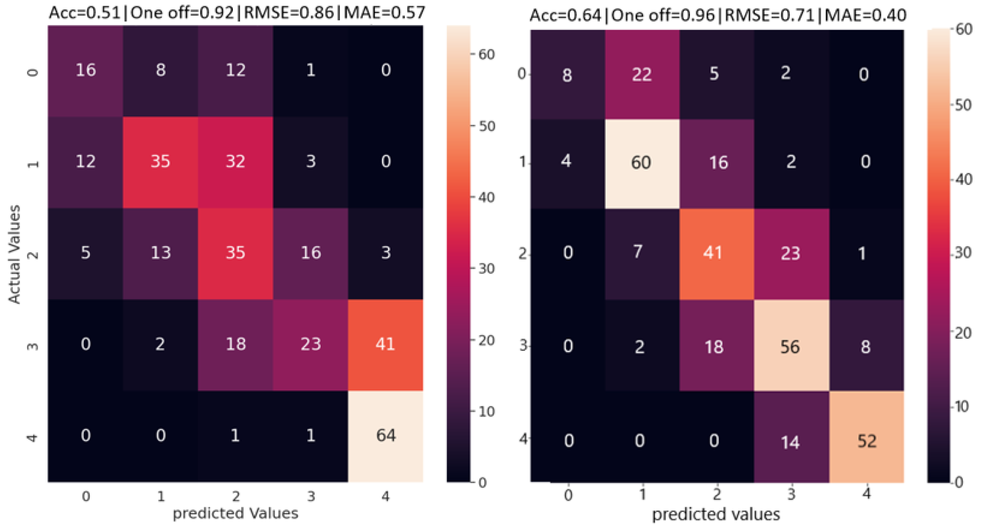
4.4. Human Variability in Annotations
Classification accuracy of deep learning models is entirely dependent on ground truth annotations provided by experts. For tasks like rating wilt levels of leaves, an absolute and precise wilt level is often difficult to determine. Thus, we wanted to quantify the extent of human variability in annotations and compare classification performance between humans and machines. In this experiment, the entire set of annotated images used for training our model was provided to the expert annotator as a reference. The task involved re-annotating the holdout test set, which consisted of 341 images. The test set was shuffled by assigning random IDs to the images. However, to create a realistic annotation scenario, the random ID was kept consistent with the date and the temporal and spatial ordering of the images were preserved. Consequently, all images taken on the same day were assigned the same random ID, with the time of day appended to it. The expert scorer was tasked with placing each image from the test set into the appropriate label folder (0–4), and a timer was used to record the time taken to annotate the entire holdout set. The re-annotated set was then compared to the original, with the latter serving as the ground truth. The re-annotated set was compared to the original set with the latter being set as the ground truth.
Figure 8 shows a comparison between performance of our MIL model and the expert scorer. We observed that the machine outperformed the human scorer not only in all classification metrics but also in scoring time per image. The machine took an average of 0.61 s to score each image, compared to 11 s on average for the human scorer. This demonstrates the advantages of applying machine learning to complex datasets, where expert decisions are often prone to error and variability. When provided with images and ground truth annotations, a machine can consistently predict the correct labels with greater accuracy and in less time than a human. Consequently, using a trained machine to assess wilt levels, rather than relying on human scorers, would significantly improve labeling consistency and efficiency.
4.5. Discussion
One of the major limitations of our work is the absence of a large-scale dataset, with our input dataset containing only 1788 annotated images. A limited sample size can pose challenges during model training, such as overfitting, and can be negatively impacted by the presence of outliers. There is also a possibility that the data may not be representative of, and hence, may not accurately reflect, the larger population it is part of. Another limitation in our dataset is class imbalance, with class 0 containing 524 instances, while class 4 has only 206 instances. This imbalance could lead to models being biased toward the majority class and performing poorly on the minority class. To address these challenges, we performed data augmentation on the training set and employed k-fold cross-validation during training (as discussed in
Section 3.3). We also used a holdout set for testing to obtain a less biased and more realistic estimate of model performance (as shown in
Section 4.2).
As part of our future work, we plan to scale up data collection to improve the classification accuracy of wilt levels. We also intend to explore unsupervised learning methods on larger datasets to eliminate any human bias during the labeling process. Lastly, we acknowledge that some variability is expected in complex datasets used in supervised machine learning, especially those involving human annotators. However, establishing a set of human annotations as the ground truth can help us train supervised models to perform more consistent and accurate annotations on new images, which is a major motivation behind our study. Furthermore, with the help of AI-assisted labeling techniques, these trained models can generate ground truth annotations, leading to more reliable labels on any new datasets collected.
5. Conclusions
Multiple instance learning can be used in the field of precision agriculture to leverage weak annotations and find key instances in the dataset. In this paper, we proposed a MIL multi-class classification model to classify leaf wilting rates in soybean plants. Our dataset only had image level annotations, but we were able to highlight key instances in images that triggered a specific bag label. We also showed that the simpler binary classification model of MIL can be changed to a multi-class model by formulating the problem as a regression task. We achieved limited accuracy on our holdout test set due to our dataset being comparatively small and having significant correlation between adjacent classes. However, our model was able to outperform DenseNet121 in most metrics, and provided comparable if performance to the state-of-the-art Vision Transformer. A comparison with human annotators showed that our model was more consistent and accurate in predicting the correct wilt level. In addition to this, our model was also able to provide interpretability in the form of heat maps. Such an approach can be useful to many researchers in the field, in tasks such as automatic weed detection, disease detection, or presence of drought stress.


 ,
, 
