Article

Investigation of Peanut Leaf Spot Detection Using Superpixel Unmixing Technology for Hyperspectral UAV Images

1
College of Computer Science and Technology, Inner Mongolia Minzu University, Tongliao 028000, China
2
College of Information and Electrical Engineering, Shenyang Agricultural University, Shenyang 110866, China
*
Author to whom correspondence should be addressed.
Agriculture 2025, 15(6), 597; https://doi.org/10.3390/agriculture15060597
Submission received: 10 February 2025 / Revised: 7 March 2025 / Accepted: 10 March 2025 / Published: 11 March 2025

Abstract

:
Leaf spot disease significantly impacts peanut growth. Timely, effective, and accurate monitoring of leaf spot severity is crucial for high-yield and high-quality peanut production. Hyperspectral technology from unmanned aerial vehicles (UAVs) is widely employed for disease detection in agricultural fields, but the low spatial resolution of imagery affects accuracy. In this study, peanuts with varying levels of leaf spot disease were detected using hyperspectral images from UAVs. Spectral features of crops and backgrounds were extracted using simple linear iterative clustering (SLIC), the homogeneity index, and k-means clustering. Abundance estimation was conducted using fully constrained least squares based on a distance strategy (D-FCLS), and crop regions were extracted through threshold segmentation. Disease severity was determined based on the average spectral reflectance of crop regions, utilizing classifiers such as XGBoost, the MLP, and the GA-SVM. Results indicate that crop spectra extracted using the superpixel-based unmixing method effectively captured spectral variability, leading to more accurate disease detection. By optimizing threshold values, a better balance between completeness and the internal variability of crop regions was achieved, allowing for the precise extraction of crop regions. Compared to other unmixing methods and manual visual interpretation techniques, the proposed method achieved excellent results, with an overall accuracy of 89.08% and a Kappa coefficient of 85.42% for the GA-SVM classifier. This method provides an objective, efficient, and accurate solution for detecting peanut leaf spot disease, offering technical support for field management with promising practical applications.

1. Introduction

The peanut (Arachis hypogaea) belongs to the legume family, and its seeds are rich in nutrients, including proteins, unsaturated fatty acids, vitamins, and minerals, making it an important crop worldwide and a significant food source [1]. Peanuts are primarily grown in tropical and subtropical regions, with the United States, China, India, Nigeria, and Senegal being the main growing countries [2]. When peanuts are infected with leaf spot disease caused by Cercosporidium personatum, the fungus colonizes the leaves and forms dark-colored spots. As the disease progresses, these spots expand continuously, causing the affected leaf tissues to wither and die. Chlorophyll in the infected areas degrades, which directly affects the plant’s ability to capture and utilize light, resulting in a reduction in peanut yield. In severe cases, the yield loss can reach up to 40% [3]. Consequently, timely, effective, and accurate monitoring of leaf spot severity is crucial for field management.
Traditional disease detection methods, such as visual evaluation, pathogen isolation, and serological tests, are subjective, time-consuming, costly, and destructive, presenting challenges for large-scale disease monitoring [4,5]. In recent years, remote sensing technology utilizing unmanned aerial vehicles (UAVs) has emerged as a promising approach for crop pest and disease monitoring due to its efficiency, cost-effectiveness, and non-invasiveness [6,7,8]. Existing studies have shown that peanut leaf spot disease can cause changes in the leaf spectrum. Specifically, the green peak (around 550 nm) associated with chlorophyll absorption weakens as the disease severity increases, while the red valley (around 670 nm) intensifies. In the near-infrared (NIR) region (around 700–1300 nm), healthy leaves usually have high reflectance. However, in infected leaves, the damaged cell structure reduces the scattering of near-infrared light, leading to a decrease in reflectance [1,9]. Disease detection at the leaf scale has high accuracy but is not conducive to large-scale disease monitoring.
Equipped with hyperspectral cameras, UAVs can achieve high spatial and temporal resolution, allowing efficient and accurate monitoring of crop health and disease distribution in the field [10,11,12,13]. Several studies have successfully detected diseases such as wheat blast, false black rice sigatoka, and wheat yellow rust using spectral, vegetation index, and texture features in hyperspectral images (His) combined with machine learning algorithms [14,15,16]. These studies have demonstrated that hyperspectral remote sensing technology provides abundant spectral and image information for crop disease detection, enabling accurate disease identification. However, existing methods often overlook the effects of background and mixed pixels on the extraction of spectral features, affecting the accuracy of disease detection.
The primary method for extracting regions of interest (ROIs) from His is manual visual interpretation [17,18,19,20]. This approach involves researchers classifying image elements based on their a priori knowledge, combined with considerations such as the size, shape, color, texture, and other features of the target region. For example, some researchers have utilized the object-based segmentation algorithm in ENVI 5.3 software to differentiate the tree canopy from the background and shadows, manually delineating the canopy region [21]. Others have acquired both hyperspectral and RGB images, mapped the canopy region in His based on the RGB image, and used the average reflectance of the vegetation region as the spectral feature of the canopy [22]. While the manual method can effectively distinguish significant heterogeneous regions, it struggles to accurately categorize transition regions and suffers from high subjectivity and low efficiency. To enhance the automation of target region extraction, researchers have employed image processing techniques for automatic extraction [23]. For instance, some researchers have identified tree canopy regions using NDVIs and morphological filtering, correcting omitted and incorrectly delineated pine regions with a watershed algorithm [24]. Others have utilized a concentric disk segmentation method for canopy segmentation and extracted reflectance spectra at the sub-plot scale [25]. Although these image segmentation methods have improved automation to some extent, segmentation accuracy is often limited because the rich spectral information embedded in His is neglected.
The spectral unmixing technique, originating from remote sensing, is a crucial method for extracting spectral information [26]. This technique effectively separates different components in His at the sub-pixel level, providing their corresponding spectral features and abundance distribution [27]. In recent years, researchers have applied the unmixing technique to extract plant information from His. For instance, the non-negative matrix factorization (NMF) method has been used to extract pure vegetation spectra from mixed tree canopy spectra, improving the extraction of key band information such as green peaks, red valleys, and red edges [28]. Unmixing methods, such as the pixel purity index (PPI) and orthogonal subspace projection, have successfully separated rice and background spectra, laying the foundation for subsequent information extraction [29]. Some studies have used vertex component analysis (VCA) to extract pure spectra from spectral images and compare the performance of different unmixing algorithms, such as least squares and K-hyper [30]. These studies have demonstrated the potential of spectral unmixing techniques for crop remote sensing using UAVs. However, existing methods often use a single endmember to represent a substance, which limits the reflection of spatial heterogeneity in crop disease symptoms and spectral feature variability.
In general, superpixel spectral unmixing is an advanced development of the traditional spectral unmixing technique. It first divides the hyperspectral image into multiple superpixels through superpixel segmentation algorithms. These superpixels are composed of adjacent pixels with similar spectral and spatial characteristics, which can reduce the complexity of data processing and better capture the local structure of the image. Then, spectral unmixing is carried out on these superpixels to obtain more accurate endmembers and abundance information. Using this method can address the issue of reflecting the spatial heterogeneity of crop disease symptoms and the variability of spectral features. Therefore, this study proposes a novel method based on superpixel spectral unmixing to accurately extract spectral features of crop regions from His for peanut plants infected with varying severities of leaf spot disease in the field. First, crops and background spectra are extracted from the images through superpixel segmentation, endmember extraction, and clustering. Second, abundance maps of the crops and background are obtained using abundance estimation, and these maps are converted into classification maps through threshold segmentation. Finally, a classification model for the average spectral features of crop regions and disease severity levels is established using multiple machine learning methods to achieve the accurate detection of peanut leaf spot disease. Compared to traditional manual visual interpretation, this method is more objective, precise, and efficient in extracting crop regions, thereby improving detection accuracy. This study aims to provide technical support for the application of hyperspectral remote sensing by UAVs in precision agriculture.

2. Materials and Methods

2.1. Study Area and Experimental Details

The experimental site for this study was located at the Haicheng Campus Test Base of Shenyang Agricultural University in Gengzhuang Town, Haicheng City, Anshan City, Liaoning Province, China (40°58′42.6′′ N to 40°58′43.68′′ N, 122°43′24.96′′ E to 122°43′29.28′′ E, 13 m above sea level). Climate-wise, the region experiences a temperate continental monsoon climate. The average annual temperature hovers around 9 °C. The annual precipitation is approximately 700–800 mm, with the majority falling in summer. The frost-free period lasts around 170 days. The high-temperature and rainy summers in this climate zone not only provide suitable conditions for peanut growth but also create a favorable environment for the occurrence and spread of peanut leaf spot disease. In terms of soil, it is loam with a pH value ranging from 6.5 to 7.5. This type of soil has excellent air-permeability and water-holding capacity and is rich in nutrients, which is highly beneficial for the growth of peanut plants. This study focused on the peanut variety “Four-Grain Red”, commonly grown in the area and susceptible to leaf spot disease. Peanuts were planted on 20 May 2021, with a row spacing of 45 cm and a plant spacing of 35 cm, covering approximately 1200 m2. Prior to planting, 81 kg of N-P2O5-K2O fertilizer per hectare was applied, and local agronomic practices were followed to control weeds, pests, and diseases. From the end of July, sustained temperatures exceeding 30 °C, coupled with increased rainfall, led to the appearance of the first symptoms of leaf spot disease in the field. By mid-August, symptoms of leaf spot had appeared with varying degrees of severity as the disease spread. As part of this study, hyperspectral and RGB images of the field were collected from August 15 to 23, and a field survey of the disease was conducted.

2.2. Data Acquisition

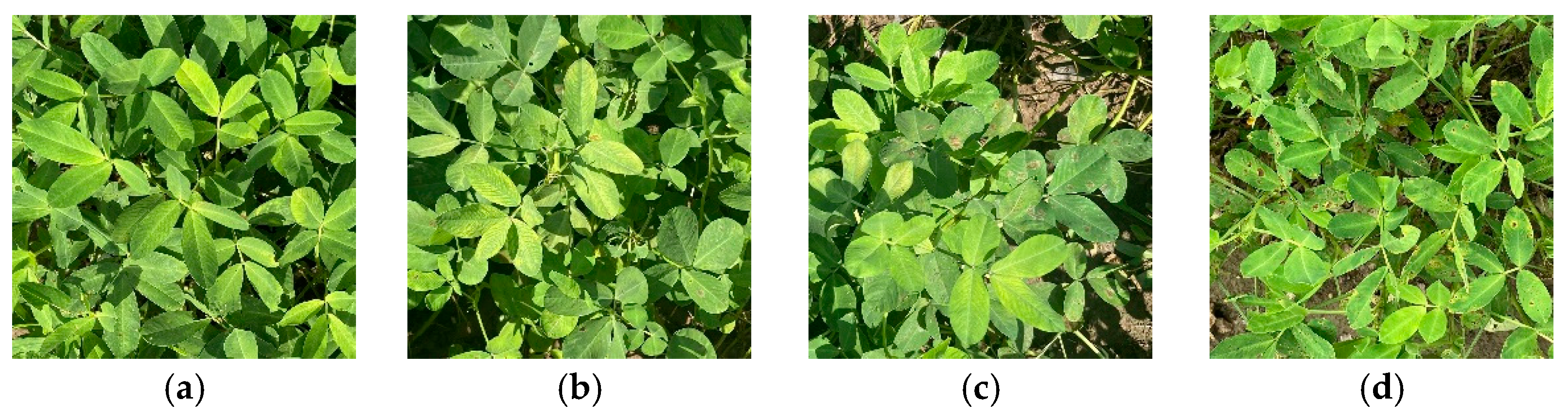
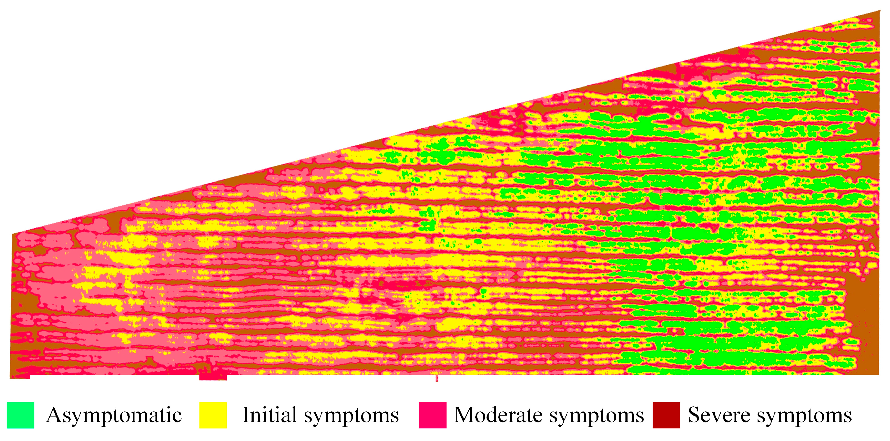
2.2.1. Disease Levels

Studies in the literature [31,32] have delved deep into the classification of the severity of crop diseases. They have categorized the diseases according to the proportion of the leaf lesion area to the total leaf area. Therefore, drawing on the findings of these studies, this research categorizes crop diseases into four levels, asymptomatic (0%), initial symptoms (0–10%), moderate symptoms (11–25%), and severe symptoms (26–50%), and leaf images at different disease levels are shown in Figure 1.
This study defined the canopy disease class using the Disease Index (DI), calculated using Equation (1) [33].
D I = 0 × n 0 + 0.1 × n 1 + 0.25 × n 2 + 0.5 × n 3 n 0 + n 1 + n 2 + n 3
where n 0 , n 1   n 2 , and n 3 denote the number of asymptomatic leaves, the number of leaves with initial symptoms, the number of leaves with moderate symptoms, and the number of leaves with severe symptoms, respectively, and their unit is “number of leaves”. Based on the DI values calculated using the above equation, the criteria for classifying the canopy disease classes are presented in Table 1, and canopy images at different disease levels are shown in Figure 2.

2.2.2. Hyperspectral Image Acquisition

An M600 PRO UAV platform with six rotors (SZ DJI Technology Co., Ltd., Shenzhen, China), equipped with a GaiaSky-mini hyperspectral imaging system (Sichuan Shuangli-hepu Science and Technology Co., Ltd., Chengde, China), was used for this study. The imaging system operated in an effective wavelength range of 400–1000 nm, consisting of 176 bands and a spectral resolution of 3.5 nm. The UAV operated at an altitude of 100 m, achieving a ground resolution of approximately 5 cm. Hyperspectral data acquisition was performed between 12:00 and 12:30 to minimize measurement errors in the His caused by variations in the sun’s elevation angle.
A hyperspectral imager was used to acquire standard white plates with reflectance greater than 99% and to obtain instrumental background noise spectral data for reflectance calibration. The reflectance of each pixel in the hyperspectral image was calculated using Equation (2):
ρ = L L d a r k L w h i t e L d a r k × ρ w h i t e
where L is the measured radiance of the pixel, L d a r k is the dark-current radiance, L w h i t e is the radiance of the white reference, and ρ w h i t e is the known reflectance of the white plate. Secondly, for lens correction, the process was completed using the internal parameters of the GaiaSky-mini hyperspectral imaging system, which compensated for the potential radial and tangential distortions of the lens. Finally, for atmospheric correction, 1.5 m × 1.5 m diffuse reflectance plates with a reflectance of 60% were set up in each hyperspectral acquisition area for reflectance data calibration.
Finally, for atmospheric correction, in each hyperspectral acquisition area, 1.5 m × 1.5 m diffuse reflectance plates with a reflectance of 60% were set up. The radiance L p a n e l of these plates was measured. We assume a linear relationship between the surface reflectance ρ and the measured radiance L of the form ρ = a × L + b . By selecting at least two non-collinear diffuse reflectance plates, we can substitute their measured radiance L p a n e l and known reflectance (60% in this case) into the equation ρ = a × L + b to solve for the coefficients a and b . Then, for each pixel in the hyperspectral image, the atmospherically corrected reflectance ρ is calculated using Equation (3).
ρ = a × L p a n e l + b
The acquired His were preprocessed in SpectralVIEW 2.9.2 software(Headwall Photonics, Fitchburg, MA, USA). Besides lens correction, reflectance correction, and atmospheric correction, the software automatically carried out a curve-smoothing operation on the spectral data, resulting in the smooth spectral signatures presented in our study.

2.2.3. Disease Marker Area Acquisition

Experts conducted disease assessments in the test field one hour before the UAV recorded the His. Crops with varying levels of disease were marked using different colored markers (blue, yellow, pink, and red). To prevent interference with the crop area’s spectrum, the markers were placed 30 cm from the north side of the crop area. The limited resolution of His leads to distortions in identifying marker colors in false-color images. Therefore, high-resolution RGB images were simultaneously captured in this study. The marker area was localized and extracted from the His using RGB images, as shown in Figure 3. A total of 586 regions were labeled in the images, including 148 asymptomatic samples, 157 with initial symptoms, 138 with moderate symptoms, and 143 with severe symptoms.

2.3. Crop Spectral Feature Extraction Method Based on Unmixing Technique

2.3.1. Superpixel Segmentation

His contain vast amounts of data and are computationally intensive to process directly. Superpixel segmentation techniques can significantly reduce computational effort by grouping neighboring pixels with similar features into homogeneous regions, thus increasing computational efficiency. Common superpixel algorithms include entropy rate-based segmentation (ERS) [34], simple linear iterative clustering (SLIC) [35], and quadtree (QT) [36]. The SLIC algorithm offers high computational speed, good precision, and strong boundary recall. It achieves this by performing local k-means clustering in a high-dimensional space to group spatially neighboring and spectrally similar pixels into superpixels. Moreover, it is easily applicable to multiple spectral bands [37]. Therefore, in this study, superpixel segmentation of His was performed using the SLIC algorithm. The number of segments was determined using an objective, entropy-based evaluation method [26].

2.3.2. Endmember Extraction

Endmember extraction aims to identify pixels with independent, pure spectral features from an image, providing the basis for subsequent spectral unmixing. In this study, the homogeneity index was used for endmember extraction. A smaller homogeneity index indicates higher pixel purity, making it more likely to be selected as an endmember [38]. Euclidean distance (ED) and spectral angular distance (SAD) were used as similarity metrics to calculate the homogeneity index of each pixel and its neighbors. The pixel with the smallest homogeneity index in each region was identified as the region’s endmember, as shown in Equation (4). To ensure efficient calculations while considering both spatial and spectral information, the neighborhood radius was set to 8 in this study. Moreover, the effectiveness of using the homogeneity index for endmember extraction has been demonstrated in relevant studies. For instance, in reference [38], this method was adopted and validated. Similarly, reference [29] also employed this approach to prove its efficacy. Using the homogeneity index for endmember extraction not only extracted pure spectral features but also preserved spatial location information for the subsequent optimization of abundance estimation.
h o m o g e n e i t y   i n d e x x = max i = 1 L x i y i 2 2 + cos 1 x T y x · y         y x m
where x is the spectral feature of pixel x , y is the spectral feature of an adjacent pixel to x , x i and y i are the values of the ith wavelength of x and y , respectively, and x m is the neighborhood of x .

2.3.3. Endmember Clustering

Since the His collected by the drone covered the entire peanut acreage in the field, this study assumed that the image contained only two types of ground. Therefore, the extracted endmembers were classified into two classes, plant endmembers and background endmembers, using the k-means clustering algorithm (k = 2). Using endmember classes helps preserve the spectral variability of crops and background, avoiding information loss that can occur when selecting a single endmember [39].

2.3.4. Abundance Estimation

Fully constrained least squares (FCLS) is a commonly used method for abundance estimation in unmixing problems. It estimates the abundance of each pixel by minimizing the difference between the reconstructed and original spectra, subject to the constraint that the sum of the abundances equals 1 and is non-negative [40]. However, traditional FCLS treats all endmembers equally, ignoring the varying contributions of each endmember to the target pixel. To address this, an improved FCLS algorithm, distance-based FCLS (D-FCLS), has been proposed in the literature. D-FCLS calculates the distance between the target pixel and each endmember, selects a subset of endmembers with the smallest distances, and re-estimates abundance based on this subset, as shown in Equation (5) [26]. This approach minimizes the influence of anomalous endmembers, which are far from the target pixel, on abundance estimation.
s j ^ = arg min s j > 0 ,   s j T 1 = 1 y j A j s j 2 2 A j A
Here, y j represents the spectral feature of pixel j , A is the matrix containing all endmembers, and s j is the abundance vector of pixel j . The constraint   s j > 0 represents abundance non-negativity constraint (ANC), and the constraint   s j T 1 = 1 represents abundance sum-to-one constraint (ASC). A j is a subset of A, where the endmembers of A j adhere to the distance strategy. The abundance of crops and background for each pixel was obtained using D-FCLS. The resulting abundance map was transformed into a classification map by applying a threshold value. Additionally, a 3 × 3 median filter was applied to remove any small, discrete noise that may have been present in the classification result. Finally, the average spectral reflectance of the crop area, extracted from the classification map, was used as the spectral feature of the crop.

2.4. Classification Methods

2.4.1. Extreme Gradient Boosting

Extreme gradient boosting (XGBoost), a gradient boosting decision tree method, automatically learns higher-order feature combinations and has a high tolerance for missing values and outliers. These properties make it suitable for processing high-dimensional and heterogeneous remote sensing data [41]. In this study, boosting calculations were performed using the gbtree method. Linear regression was used as the objective function, with classification error as the evaluation metric. A learning rate of 0.05 was set, and the optimal number of decision trees was determined through cross-validation. The optimization process involved fitting a new decision tree to the residuals of the previous model in each iteration, and we balanced model complexity and performance by adjusting the learning rate and tree number via cross-validation.

2.4.2. Multi-Layer Perceptron

The multi-layer perceptron (MLP) is a commonly used artificial neural network model with input, hidden, and output layers. It effectively captures complex non-linear decision boundaries and is widely used in pattern recognition and other fields [42]. In this study, a feed-forward MLP network with 20 hidden layers was constructed. The network employed the ReLU activation function and the Adam optimization algorithm with a learning rate of 0.01 and a batch size of 32. It ran for a maximum of 1000 iterations. The optimal network model was obtained through back-propagation, where the Adam algorithm adjusted the weights based on the gradients of the error.

2.4.3. Support Vector Machine Based on Genetic Algorithm

The Support Vector Machine (SVM) has excellent generalization ability and performs well on classification problems with small sample sizes, but it is sensitive to hyperparameter selection, such as the kernel function and penalty parameters [43]. In this study, a genetic algorithm (GA) was used to optimize the SVM parameters. The GA had a population size of 20, a maximum of 200 iterations, a search range for the penalty parameter C and the kernel function parameter γ of [0, 100], and a crossover probability of 0.9. The SVM used the Radial Basis Function (RBF) kernel. The GA started with an initial population, evaluated fitness on a validation set, selected the best candidates, and applied genetic operators. This process repeated until the optimal C and γ were found, and then the SVM network was trained with these optimal parameters.

2.5. Evaluation Indicators

In this study, two evaluation metrics, overall accuracy (OA) and the Kappa coefficient (Kappa), were used to comprehensively and objectively assess the classification performance of the proposed method [32]. OA represents the proportion of samples that are correctly classified, and its calculation is shown in Equation (6).
O A = T P + T N T P + F N + F P + T N
where T P , T N , F P , and F N denote the number of true positive cases, true negative cases, false positive cases, and false negative cases, respectively. A higher OA value indicates the higher classification accuracy of the model. However, OA alone cannot represent the distribution of samples in each category. When there is an imbalance in the data distribution, OA evaluation tends to be biased. To address this issue, the study adopted Kappa as an additional evaluation metric. Kappa corrects for the chance accuracy caused by random factors and can more objectively reflect the degree of consistency between the classification results and the true labels, as shown in Equation (7).
K a p p a = P o P e 1 P e
where P o is the observed accuracy and P e is the expected accuracy. Kappa ranges from −1 to 1; the closer the value is to 1, the greater the consistency between the classification results and the true labels is, whereas a value of 0 indicates that the classification accuracy is no better than random chance.

2.6. Flow of Disease Detection Method Based on Superpixel Unmixing Technique

This study employed a superpixel-based unmixing technique for detecting peanut leaf spot disease, as shown in Figure 4. First, a field disease survey labeled crops with varying disease severity, and hyperspectral UAV and high-resolution RGB images were collected. The original His were then preprocessed and combined with high-resolution RGB images to extract labeled regions. Superpixel segmentation was performed on the His to group similar neighboring pixels into homogeneous regions, reducing the processing load. Endmember extraction was performed on the superpixels, with pixels with the smallest homogeneity index identified as endmembers. The endmembers were classified into crop and background classes using a clustering algorithm. Abundance estimation was then carried out using D-FCLS to generate the abundance map. The resulting abundance map was converted into a classification map by applying a threshold. Finally, the average spectra of crop regions and labeled disease levels were used to construct the detection model for peanut leaf spot disease. The model’s performance was assessed using overall OA and Kappa.

3. Results and Analysis

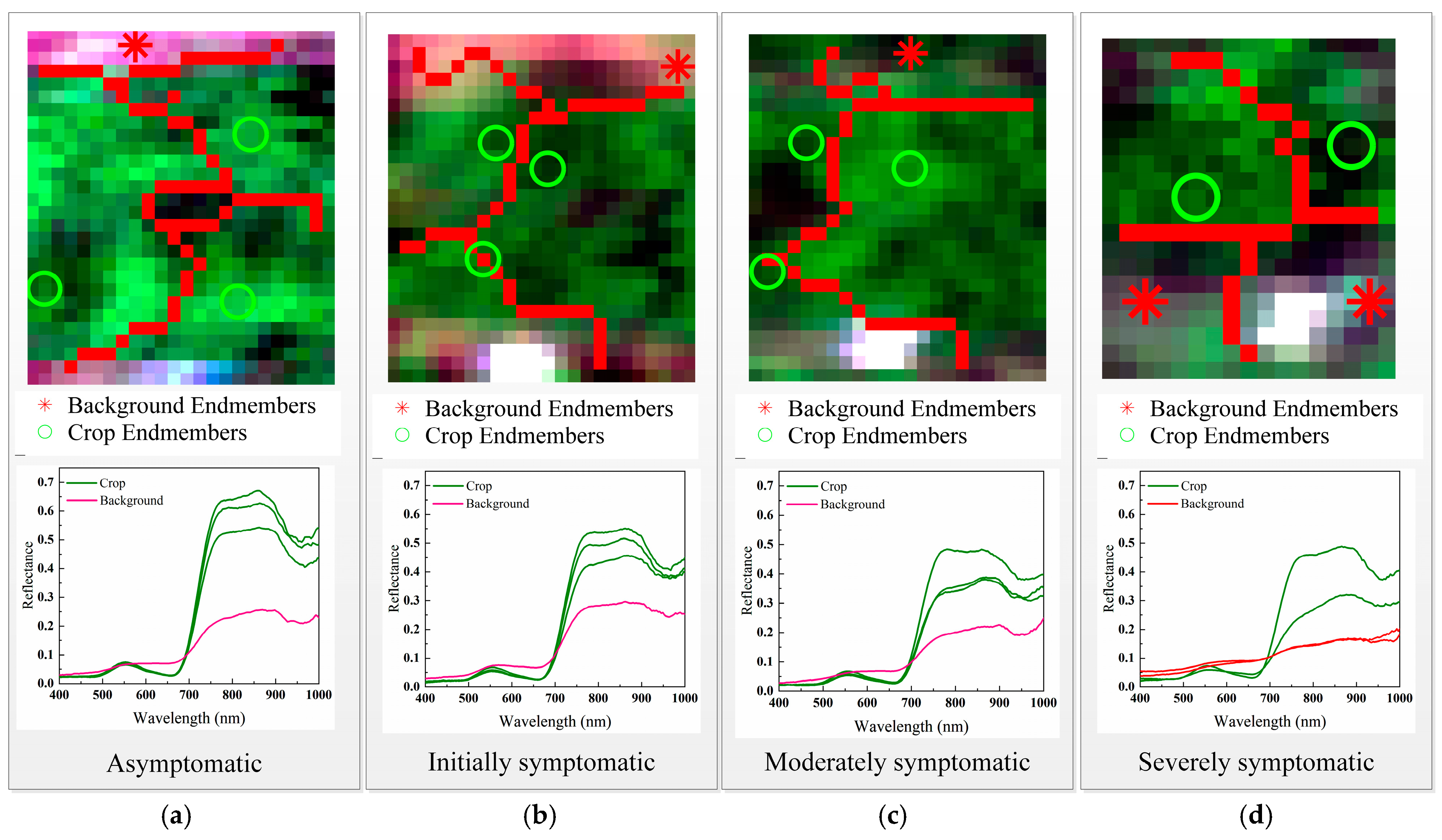
3.1. Spectral Feature Extraction Results

To evaluate the performance of the proposed disease detection method based on the superpixel unmixing technique, marked regions representing different disease severities were selected from hyperspectral images (His) for testing. Before the UAV captured the His, experts conducted disease assessments in the test field. Crops with varying disease levels were marked with specific-colored markers: blue for asymptomatic crops, yellow for those in the early stage of the disease, pink for moderately affected crops, and red for severely affected ones. However, due to the limited resolution and distortion during the conversion of His to pseudo-color images, and the 14.6-fold magnification for better sub-region extraction, the original colors of the markers cannot be accurately presented in the false-color images shown in Figure 5.
Figure 5 presents false-color images of regions with different disease classes extracted from the original His. The marked regions are circled with red frames. To address the issue of color distortion of the markers and obtain accurate disease information, high-resolution RGB images were simultaneously collected for calibration. The specific methods for acquiring and calibrating the disease-marked areas are detailed in Section 2.2.3.
The images underwent processing using superpixel segmentation, endmember extraction, and endmember clustering, as shown in Figure 6. In Figure 6, the circle represents crop endmembers, the asterisk represents background endmembers, and the red line represents the results of superpixel segmentation. The superpixel segmentation algorithm (SLIC) effectively grouped similar pixels into homogeneous small regions, producing regions that were more uniform in shape, size, and distribution. Extracting an endmember from a superpixel effectively avoided extracting mixed pixels. The extracted spectral features revealed differences in spectral characteristics across different locations of the same crop. The variability in crop spectra could be effectively represented using the endmember class.
It can be observed from Figure 6 that some endmembers are located at the edges of superpixels. This might be because the endmember extraction algorithm we used is designed to identify the pixel with the minimum homogeneity index within each pixel group. In the superpixels where these edge-located endmembers are found, the other pixels are often in a transition area between different materials (such as the crop-background transition area). These pixels are severely mixed, resulting in a significantly larger homogeneity index for them. As a result, the pixel with a relatively lower homogeneity index, even if it is at the edge of the superpixel, is selected as the endmember.

3.2. Comparison of Pure and Mixed Spectral Features

In this study, a meticulous two-step process was employed for endmember extraction and average spectrum calculation. First, for each of the 586 labeled regions, which were categorized into 148 asymptomatic samples, 157 samples with initial symptoms, 138 samples with moderate symptoms, and 143 samples with severe symptoms, crop endmembers were extracted from each individual image. The number of crop endmembers per image ranged from two to three. For each image, the crop endmembers were averaged, and the resulting average spectral curve was designated as the endmember for the corresponding category of that image. Subsequently, all sub-region samples within the same category were aggregated, and their average was calculated to obtain the final average spectrum for each disease severity level. These average spectra are presented in the dashed part of Figure 7, effectively distilling the characteristic spectral features of each disease level. To analyze the effect of mixed spectra on crop spectral features, mixed spectra with different crop-to-background ratios (0.2, 0.4, 0.6, and 0.8 for the crop) were tested, as shown by the solid lines in Figure 7.
From a biological perspective, these spectral features can be closely related to the physiological changes in peanut plants caused by leaf spot disease. In the 600–700 nm (green and red) range, pure spectra of crops at different disease levels show minor differences but are significantly distinct from the mixed spectra, which exhibit higher reflectance than the pure crop spectra. According to [44], the decrease in green-band reflectance might be due to chlorophyll decomposition as the disease damages the chloroplasts. Meanwhile, the changes in red-band reflectance are likely associated with the variations in carotenoid and lutein pigments affected by the disease-disrupted physiological processes.
In the near-infrared band (700–1000 nm), the mixed spectra exhibit curves similar to those of the pure crop spectra, potentially causing interference. When the crop ratio is lower than 0.2, the mixed spectrum curve deviates significantly from the pure crop spectrum. The decrease in near-infrared reflectance, as mentioned in [45,46], is mainly due to changes in leaf structure and water content caused by the disease. The disease can damage leaf tissue and disrupt the water-transport system. Also, factors like leaf shape, transpiration rate, canopy morphology, and plant density, which are influenced by the disease, further affect the near-infrared reflectance.
Therefore, the 600–700 nm range is the best band for distinguishing pure crop spectra from mixed spectra. In the 700–1000 nm range, the difference between the two spectra significantly increases as the crop composition ratio decreases.

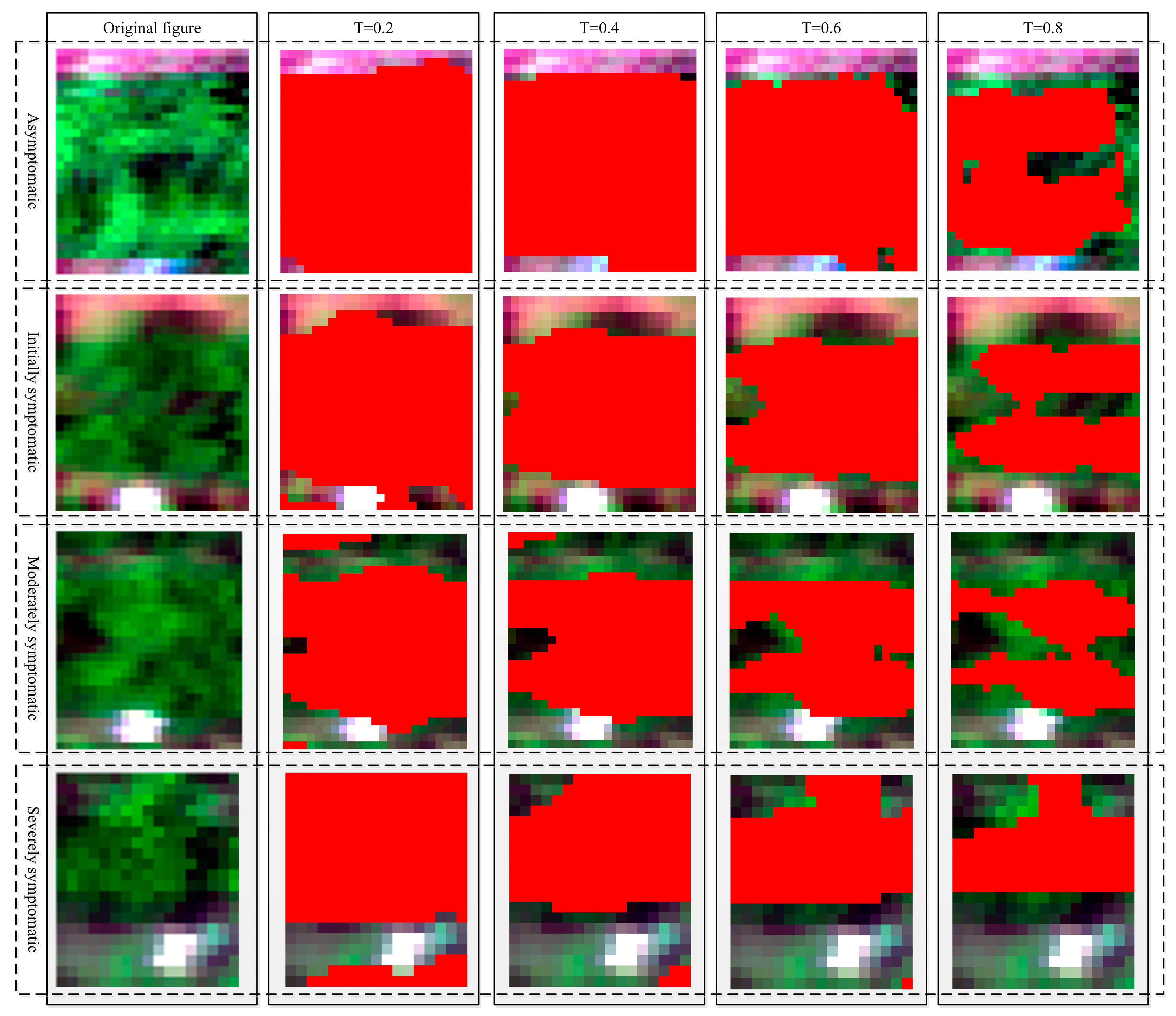
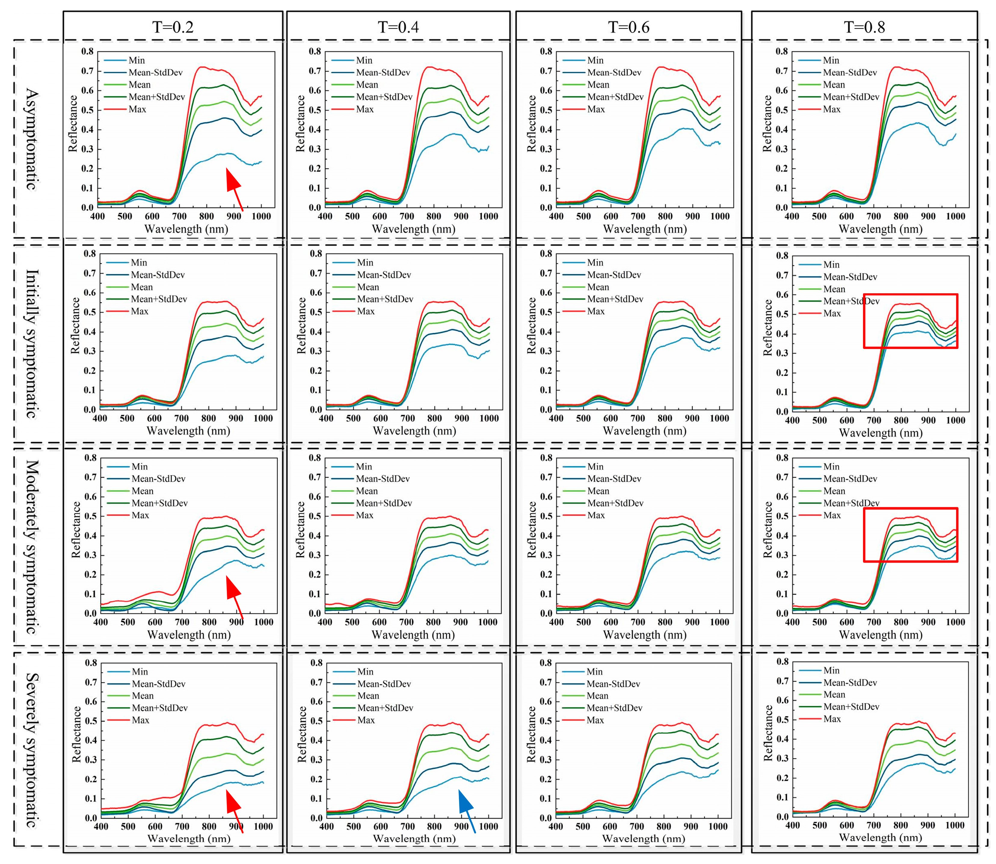
3.3. Crop Region Extraction Results

In this study, D-FCLS was used to estimate the abundance of the labeled areas. The abundance maps were then converted into classification maps of crops and background by setting different segmentation thresholds (T = 0.2, 0.4, 0.6, and 0.8). Crop areas were classified when the crop abundance exceeded T, while background areas were classified otherwise. Figure 8 illustrates crop coverage for different thresholds. The results indicate that as the threshold T increases, the extracted crop area decreases. When T is low (T = 0.2), excessive crop area is extracted, potentially including parts of the background. When T is high (T = 0.8), the extracted crop area is overly concentrated in the center, neglecting the edge area.
The maximum (Max), minimum (Min), mean (Mean), and standard deviation (StdDev) of the spectral features of the crop area were employed to evaluate the consistency of the crop area spectra for different thresholds (T), as illustrated in Figure 9. In the figure, different rows represent different disease severity levels (from top to bottom: asymptomatic, initial symptoms, moderate symptoms, and severe symptoms), and different columns represent different thresholds (from left to right: 0.2, 0.4, 0.6, and 0.8).
The Max values across different T are comparable, as are the Mean and Mean ± StdDev values. This indicates that the spectra of most crop pixels extracted by all methods are similar. At T = 0.2, the Min reflectance of asymptomatic, moderately symptomatic, and severely symptomatic crops exhibit low values and distortion in the near-infrared (NIR) band (as indicated by the red arrows in the chart). At T = 0.4, the Min reflectance of severely symptomatic crops shows significant differences and distortion in the red band (as pointed out by the blue arrows in the chart). These phenomena may be attributed to the fact that an excessively small threshold led to the excessive mixing of the background with the crops.
As shown by the curves in the chart, the StdDev decreases as the T value increases. This decline suggests a reduction in the spectral variability within the region. Given the earlier conclusion that there are significant differences between pure and mixed spectra in the red and near-infrared bands, mixed pixels are present in the regions with moderate and severe symptoms at T = 0.2 and 0.4. At T = 0.8; there are no mixed pixels, but the spectral set is overly concentrated (as shown within the red box in the figure).
T = 0.6 was the optimal threshold because it could more effectively extract the complete crop area, avoid excessive interference from mixed pixels, and maintain a moderate level of internal spectral variability. Furthermore, an examination of Figure 9 reveals that overlapping regions exist between the maximum and minimum values of spectral curves across different disease severity levels. Nevertheless, when taking into account the Mean ± StdDev values, distinct differentiations among the various disease levels become apparent. The majority of the curves do not overlap, suggesting that notwithstanding the partial overlap within the min–max range, the data retain an adequate discriminatory capacity for classification applications. This characteristic validates the utilization of the spectral data and thresholds presented in Figure 9 for the assessment of crop disease severity.

3.4. Crop Disease Detection Results

Using the aforementioned method, the average spectral reflectance of the crop was extracted from the labeled area. XGBoost, the MLP, and the GA-SVM were employed to assess the effect of different T on disease detection, with the results shown in Figure 10. Accuracy generally increased with the increase in T. This is because a larger T value reduced the influence of background pixels, making the crop’s spectral features more prominent for the classification models. However, when T = 0.8, the accuracy decreased. An overly large T may have excluded some valid crop pixels, leading to the loss of crucial spectral information for disease detection.
All models achieved higher accuracy at T = 0.6. At this threshold, they could effectively extract a relatively complete crop area, avoiding excessive interference from background pixels and retaining sufficient spectral information. This enabled the classification models to perform more accurate disease classification. In conclusion, after evaluating different threshold values of T both qualitatively and quantitatively, this study determined that T = 0.6 was the optimal segmentation threshold.

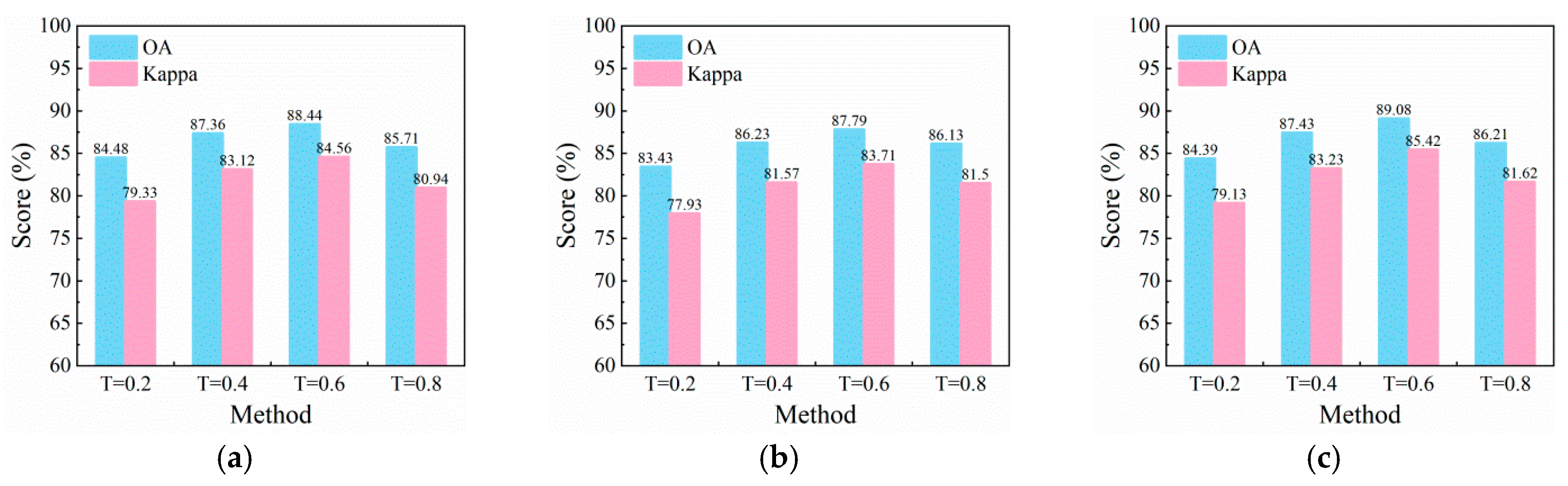
3.5. Comparison with Other Unmixing Methods

3.5.1. Comparison with Other Superpixel Methods

Superpixel segmentation is a crucial step in the extraction process of vegetation regions, as it significantly impacts the accuracy of subsequent disease detection. Therefore, this study employed three superpixel segmentation algorithms—ERS [34], SLIC [35], and QT [36]—to extract crop spectra from the labeled regions. Classification models, including XGBoost, the MLP, and the GA-SVM, were then used to assess the disease detection performance of these segmentation methods. The results are shown in Table 2. The results indicate that, among the three classification models tested, the SLIC algorithm achieved the highest disease detection accuracy. Specifically, when using the GA-SVM model, OA and Kappa reached 89.08% and 85.42%, respectively, indicating optimal detection performance.

3.5.2. Comparison with Other Abundance Estimation Methods

The D-FCLS method was compared with SPU [47], MESMA [48], FCLS [40], MD-FCLS [26], Mean-FCLS [49], D-SPU [26], and D-MESMA [26] based on disease detection accuracy and computational efficiency (average runtime per pixel). The results are shown in Table 3. Although MESMA achieved the highest OA and Kappa, its computational efficiency was significantly lower than that of other methods, making it less suitable for practical applications. In contrast, D-FCLS achieved a detection accuracy comparable to that of MESMA across all three classifiers, with an average runtime of 0.00081 s/pixel, significantly lower than MESMA’s (0.0053 s/pixel). Thus, the D-FCLS method outperformed other abundance estimation methods in both detection accuracy and efficiency.

3.6. Comparison Results with Traditional Region-of-Interest Extraction Methods

This study compared disease detection accuracy using ellipse, rectangle, and polygon extractors in ENVI 5.6 software (Harris Geospatial, Boulder, CO, USA) with the superpixel unmixing technique proposed in this paper [50]. The results are shown in Table 4. The results show that the crop region extraction method based on the superpixel unmixing technique achieved the highest disease detection accuracy with all three classifiers. In contrast, the elliptical extractor method had the lowest detection accuracy, with OA and Kappa around 78%. The detection accuracies of the rectangular and polygonal extractors were higher but still lower than that of the proposed method. Thus, the disease detection method based on superpixel unmixing proposed in this study is superior to manual visual interpretation.

4. Discussion

This study employed a superpixel-based unmixing method to delineate crop regions in His and extract their spectral features for detecting peanut leaf spot disease severity. The non-uniform distribution of peanut leaf spot disease within the same plant, along with the inability of local disease conditions to represent overall disease severity, prompted the use of this method. Analysis of endmember extraction results revealed spectral differences across various locations within the crop area, consistent with actual disease occurrences. To accurately assess disease occurrences in crops, this study employed spectral unmixing to delineate the entire crop region, using the average spectral reflectance as its spectral feature. The studies [51,52] found differences in leaf spectra at different positions of crops. This conclusion aligns with that of the present study. This study also investigated the impact of mixed pixel spectra on the spectral features of vegetation at various disease levels. The findings indicate that mixed spectra of crops and soil resembled crop disease spectra and could interfere with crop spectra, affecting disease detection accuracy. A study on detecting the distribution of salt marsh plant species using UAV hyperspectral imaging found that spectra in species transition zones were variably mixed, leading to reduced detection accuracy [53]. Therefore, the precise separation and extraction of crop regions from His are crucial for accurate disease detection.
To accurately extract the spectral features of the crop area, this study examined the impact of varying segmentation thresholds (T) on the accuracy of crop region extraction, considering the overlap between mixed pixels of crops, background, and disease spectra. The results indicated that a small T could lead to the misclassification of soil and mixed regions as crop areas. Conversely, a large T led to incomplete crop region extraction, complicating the accurate delineation of actual disease occurrences. This study conducted a statistical analysis of crop spectral features at different T levels. The analysis assessed spectral anomalies using Max and Min, overall spectral characteristics using Mean ± StdDev, and spectral distribution consistency using StdDev. The findings suggested that a small T altered the shape of the Min curve, indicating potential interference from background or mixed pixels in the extracted region. Conversely, a large T, leading to a small StdDev value, indicated an overly concentrated extracted area that may have failed to cover all crop areas. Additionally, this study used classifiers such as XGBoost, the MLP, and the GA-SVM to evaluate disease detection performance for different T values. The results showed that the highest detection accuracy for all classifiers occurred at T = 0.6. Based on a comprehensive qualitative and quantitative analysis, this study concluded that T = 0.6 was the optimal segmentation threshold. This threshold ensured a balanced representation of the crop area, preserving both integrity and internal variability, and provided high-quality input features for subsequent disease detection. In the literature [54,55], thresholds of 70% and 50% have been used for category classification. This difference arises from the different research objects.
This study employed the unmixing technique to automatically identify the crop region, minimizing the influence of background and mixed pixels and achieving high detection accuracy. A comparative analysis with commonly used superpixel and abundance estimation methods showed that the method proposed in this study outperformed them in terms of accuracy and operational efficiency. The comparison with commonly used manual extraction methods indicated that the method proposed in this study performed better. These results can be attributed to the limitations of the elliptical extraction method, which is constrained by the shape of the extraction area and can only extract spectral features from the crop’s central region, while the actual disease often occurs on the outer edges. The rectangular extraction method is prone to interference from background information, making it difficult to distinguish the crop from the background. The polygonal extraction method relies on manual selection, which may lead to the subjective choice of pixel points with prominent features, potentially overlooking pixels with less distinct color features in areas severely affected by the disease. Therefore, the method proposed in this study achieves objective, accurate, and efficient crop region extraction, facilitating disease severity detection.
In addition, this study utilized the established classification model to achieve visualization of hyperspectral images, and the results are shown in Figure 11. In this figure, green represents asymptomatic, yellow represents initial symptoms, pink represents moderate symptoms, and red represents severe symptoms. Each pixel in the image was classified into a disease severity level or the background, and a 3 × 3 filter was used to smooth the classification map. As can be seen from Figure 11, the regions of different disease levels are relatively evenly distributed, the regions with the same disease level are continuous, and the regions with similar disease levels are also relatively close in the figure. These situations are more in line with the actual occurrence.

5. Conclusions

This study employed a superpixel-based spectral unmixing approach to detect peanut leaf spot disease. Initially, a field survey was conducted to label crops according to their disease severity levels. Subsequently, an unmanned aerial vehicle (UAV) was utilized to collect hyperspectral images (His) and high-resolution RGB images. After preprocessing the His, they were integrated with the RGB images to extract the labeled regions. Next, superpixel segmentation was carried out to group similar pixels together. Endmember extraction followed, and the endmembers were classified into crop and background categories. The D-FCLS method was applied to estimate the endmember abundances, and a threshold was used to convert the abundance map into a classification map. Crop regions with varying disease severities were extracted, and their average spectral features were calculated. The accuracy of the proposed peanut leaf spot disease detection method was evaluated using various machine learning techniques.
The results indicate that the crop endmembers obtained through superpixel segmentation, endmember extraction, and clustering could comprehensively and accurately represent the spectral characteristics of the crops. Determining the optimal threshold enabled the accurate extraction of crop regions, providing precise features for disease detection.
The proposed method was compared with other unmixing and manual visual interpretation methods using classifiers such as XGBoost, the MLP, and the GA-SVM. When using the GA-SVM classifier, the proposed method achieved an overall accuracy (OA) of 89.08% and a Kappa coefficient of 85.42%.
In comparison with other superpixel segmentation algorithms (ERS, SLIC, and QT), the SLIC algorithm used in our method showed the best performance. For instance, when using the GA-SVM model, ERS had an OA of 88.44% and a Kappa of 84.56% and QT had an OA of 84.48% and a Kappa of 79.33%, while our SLIC-based method outperformed them. When comparing the D-FCLS abundance estimation method with other methods (SPU, MESMA, FCLS, MD-FCLS, Mean-FCLS, D-SPU, and D-MESMA), although MESMA achieved high OA and Kappa values, its computational efficiency was significantly lower (average runtime of 0.0053 s/pixel) compared to our D-FCLS method (0.00081 s/pixel). In comparison with traditional region-of-interest extraction methods (elliptical, rectangular, and polygonal extractors in ENVI 3.5 software), the elliptical extractor method had the lowest detection accuracy (OA and Kappa around 78%), while our proposed method achieved the highest accuracy across all three classifiers.
In conclusion, the method proposed in this study enables the objective, accurate, and efficient detection of peanut leaf spot disease. This approach is advantageous for the non-destructive detection of the disease in large-scale fields and provides technical support for field-scale detection.

Author Contributions

Conceptualization, Q.G.; data curation, S.F.; formal analysis, S.Q.; funding acquisition, W.D.; investigation, Q.G.; methodology, Q.G.; project administration, W.D.; resources, W.D.; software, S.Q.; supervision, W.D.; validation, Q.G.; visualization, S.F.; writing—original draft, Q.G.; writing—review and editing, W.D. All authors have read and agreed to the published version of the manuscript.

Funding

This research was partially funded by the Doctoral Startup Foundation of Inner Mongolia (BSZ006), Basic Research Operating Expenses of Colleges and Universities directly under the Inner Mongolia Autonomous Region-Natural Science Research (GXKY25Z016), and Liaoning Provincial Department of Education Platform Project (JYTPT2024002).

Data Availability Statement

Data are contained within the article.

Conflicts of Interest

The authors declare that they have no conflicts of interest.

References

  1. Guan, Q.; Zhao, D.; Feng, S.; Xu, T.; Wang, H.; Song, K. Hyperspectral Technique for Detection of Peanut Leaf Spot Disease Based on Improved PCA Loading. Agronomy 2023, 13, 1153. [Google Scholar] [CrossRef]
  2. Khera, P.; Pandey, M.K.; Wang, H.; Feng, S.; Qiao, L.; Culbreath, A.K.; Kale, S.; Wang, J.; Holbrook, C.C.; Zhuang, W.; et al. Mapping Quantitative Trait Loci of Resistance to Tomato Spotted Wilt Virus and Leaf Spots in a Recombinant Inbred Line Population of Peanut (Arachis hypogaea L.) from SunOleic 97R and NC94022. PLoS ONE 2016, 11, e0158452. [Google Scholar] [CrossRef] [PubMed]
  3. Bera, S.K.; Rani, K.; Kamdar, J.H.; Pandey, M.K.; Desmae, H.; Holbrook, C.C.; Burow, M.D.; Manivannan, N.; Bhat, R.S.; Jasani, M.D.; et al. Genomic Designing for Biotic Stress Resistant Peanut. In Genomic Designing for Biotic Stress Resistant Oilseed Crops; Kole, C., Ed.; Springer International Publishing: Cham, Switzerland, 2022; pp. 137–214. [Google Scholar]
  4. Graham, J.H.; Leite, R.P. Lack of Control of Citrus Canker by Induced Systemic Resistance Compounds. Plant Dis. 2004, 88, 745–750. [Google Scholar] [CrossRef]
  5. Suk Park, D.; Wook Hyun, J.; Jin Park, Y.; Sun Kim, J.; Wan Kang, H.; Ho Hahn, J.; Joo Go, S. Sensitive and specific detection of Xanthomonas axonopodis pv. citri by PCR using pathovar specific primers based on hrpW gene sequences. Microbiol. Res. 2006, 161, 145–149. [Google Scholar] [CrossRef]
  6. Maes, W.H.; Steppe, K. Perspectives for Remote Sensing with Unmanned Aerial Vehicles in Precision Agriculture. Trends Plant Sci. 2019, 24, 152–164. [Google Scholar] [CrossRef]
  7. Kerkech, M.; Hafiane, A.; Canals, R. Deep leaning approach with colorimetric spaces and vegetation indices for vine diseases detection in UAV images. Comput. Electron. Agric. 2018, 155, 237–243. [Google Scholar] [CrossRef]
  8. Kuswidiyanto, L.W.; Noh, H.-H.; Han, X. Plant Disease Diagnosis Using Deep Learning Based on Aerial Hyperspectral Images: A Review. Remote Sens. 2022, 14, 6031. [Google Scholar] [CrossRef]
  9. Guan, Q.; Song, K.; Feng, S.; Yu, F.; Xu, T. Detection of Peanut Leaf Spot Disease Based on Leaf-, Plant-, and Field-Scale Hyperspectral Reflectance. Remote Sens. 2022, 14, 4988. [Google Scholar] [CrossRef]
  10. Park, S.; Nolan, A.; Ryu, D.; Fuentes, S.; Hernandez, E.; Chung, H.; O’Connell, M. Estimation of crop water stress in a nectarine orchard using high-resolution imagery from unmanned aerial vehicle (UAV). In Proceedings of the 21st International Congress on Modelling and Simulation, Gold Coast, Australia, 29 November–4 December 2015. [Google Scholar]
  11. Bendig, J.; Yu, K.; Aasen, H.; Bolten, A.; Bennertz, S.; Broscheit, J.; Gnyp, M.L.; Bareth, G. Combining UAV-based plant height from crop surface models, visible, and near infrared vegetation indices for biomass monitoring in barley. Int. J. Appl. Earth Obs. Geoinf. 2015, 39, 79–87. [Google Scholar] [CrossRef]
  12. Calderón, R.; Navas-Cortés, J.A.; Zarco-Tejada, P.J. Early Detection and Quantification of Verticillium Wilt in Olive Using Hyperspectral and Thermal Imagery over Large Areas. Remote Sens. 2015, 7, 5584–5610. [Google Scholar] [CrossRef]
  13. Zhang, J.; Huang, Y.; Pu, R.; Gonzalez-Moreno, P.; Yuan, L.; Wu, K.; Huang, W. Monitoring plant diseases and pests through remote sensing technology: A review. Comput. Electron. Agric. 2019, 165, 104943. [Google Scholar] [CrossRef]
  14. Ma, H.; Huang, W.; Dong, Y.; Liu, L.; Guo, A. Using UAV-Based Hyperspectral Imagery to Detect Winter Wheat Fusarium Head Blight. Remote Sens. 2021, 13, 3024. [Google Scholar] [CrossRef]
  15. An, G.; Xing, M.; He, B.; Kang, H.; Shang, J.; Liao, C.; Huang, X.; Zhang, H. Extraction of Areas of Rice False Smut Infection Using UAV Hyperspectral Data. Remote Sens. 2021, 13, 3185. [Google Scholar] [CrossRef]
  16. Guo, A.; Huang, W.; Dong, Y.; Ye, H.; Ma, H.; Liu, B.; Wu, W.; Ren, Y.; Ruan, C.; Geng, Y. Wheat Yellow Rust Detection Using UAV-Based Hyperspectral Technology. Remote Sens. 2021, 13, 123. [Google Scholar] [CrossRef]
  17. Zhang, S.; Li, X.; Ba, Y.; Lyu, X.; Zhang, M.; Li, M. Banana Fusarium Wilt Disease Detection by Supervised and Unsupervised Methods from UAV-Based Multispectral Imagery. Remote Sens. 2022, 14, 1231. [Google Scholar] [CrossRef]
  18. Zhang, H.; Huang, L.; Huang, W.; Dong, Y.; Weng, S.; Zhao, J.; Ma, H.; Liu, L. Detection of wheat Fusarium head blight using UAV-based spectral and image feature fusion. Front. Plant Sci. 2022, 13, 1004427. [Google Scholar] [CrossRef]
  19. Wang, Y.; Xing, M.; Zhang, H.; He, B.; Zhang, Y. Rice False Smut Monitoring Based on Band Selection of UAV Hyperspectral Data. Remote Sens. 2023, 15, 2961. [Google Scholar] [CrossRef]
  20. Zhao, D.; Cao, Y.; Li, J.; Cao, Q.; Li, J.; Guo, F.; Feng, S.; Xu, T. Early Detection of Rice Leaf Blast Disease Using Unmanned Aerial Vehicle Remote Sensing: A Novel Approach Integrating a New Spectral Vegetation Index and Machine Learning. Agronomy 2024, 14, 602. [Google Scholar] [CrossRef]
  21. Yu, R.; Ren, L.; Luo, Y. Early detection of pine wilt disease in Pinus tabuliformis in North China using a field portable spectrometer and UAV-based hyperspectral imagery. For. Ecosyst. 2021, 8, 44. [Google Scholar] [CrossRef]
  22. Zhang, N.; Zhang, X.; Yang, G.; Zhu, C.; Huo, L.; Feng, H. Assessment of defoliation during the Dendrolimus tabulaeformis Tsai et Liu disaster outbreak using UAV-based hyperspectral images. Remote Sens. Environ. 2018, 217, 323–339. [Google Scholar] [CrossRef]
  23. Zhang, N.; Wang, Y.; Zhang, X. Extraction of tree crowns damaged by Dendrolimus tabulaeformis Tsai et Liu via spectral-spatial classification using UAV-based hyperspectral images. Plant Methods 2020, 16, 135. [Google Scholar] [CrossRef] [PubMed]
  24. Zhang, S.; Huang, H.; Huang, Y.; Cheng, D.; Huang, J. A GA and SVM Classification Model for Pine Wilt Disease Detection Using UAV-Based Hyperspectral Imagery. Appl. Sci. 2022, 12, 6676. [Google Scholar] [CrossRef]
  25. Kurihara, J.; Koo, V.-C.; Guey, C.W.; Lee, Y.P.; Abidin, H. Early Detection of Basal Stem Rot Disease in Oil Palm Tree Using Unmanned Aerial Vehicle-Based Hyperspectral Imaging. Remote Sens. 2022, 14, 799. [Google Scholar] [CrossRef]
  26. Guan, Q.; Xu, T.; Feng, S.; Yu, F.; Song, K. Optimal segmentation and improved abundance estimation for superpixel-based Hyperspectral Unmixing. Eur. J. Remote Sens. 2022, 55, 485–506. [Google Scholar] [CrossRef]
  27. Bioucas-Dias, J.M.; Plaza, A.; Dobigeon, N.; Parente, M.; Du, Q.; Gader, P.; Chanussot, J. Hyperspectral Unmixing Overview: Geometrical, Statistical, and Sparse Regression-Based Approaches. IEEE J. Sel. Top. Appl. Earth Obs. Remote Sens. 2012, 5, 354–379. [Google Scholar] [CrossRef]
  28. Lu, J.; Li, W.; Yu, M.; Zhang, X.; Ma, Y.; Su, X.; Yao, X.; Cheng, T.; Zhu, Y.; Cao, W.; et al. Estimation of rice plant potassium accumulation based on non-negative matrix factorization using hyperspectral reflectance. Precis. Agric. 2021, 22, 51–74. [Google Scholar] [CrossRef]
  29. Yu, F.; Bai, J.; Jin, Z.; Zhang, H.; Guo, Z.; Chen, C. Research on Precise Fertilization Method of Rice Tillering Stage Based on UAV Hyperspectral Remote Sensing Prescription Map. Agronomy 2022, 12, 2893. [Google Scholar] [CrossRef]
  30. Pölönen, I.; Saari, H.; Kaivosoja, J.; Honkavaara, E.; Pesonen, L. Hyperspectral imaging based biomass and nitrogen content estimations from light-weight UAV. In Proceedings of the SPIE Remote Sensing 2013, Dresden, Germany, 23–26 September 2013; p. 88870J. [Google Scholar]
  31. Bauriegel, E.; Giebel, A.; Geyer, M.; Schmidt, U.; Herppich, W.B. Early detection of Fusarium infection in wheat using hyper-spectral imaging. Comput. Electron. Agric. 2011, 75, 304–312. [Google Scholar] [CrossRef]
  32. Chen, T.; Yang, W.; Zhang, H.; Zhu, B.; Zeng, R.; Wang, X.; Wang, S.; Wang, L.; Qi, H.; Lan, Y.; et al. Early detection of bacterial wilt in peanut plants through leaf-level hyperspectral and unmanned aerial vehicle data. Comput. Electron. Agric. 2020, 177, 105708. [Google Scholar] [CrossRef]
  33. Huang, W.; Lamb, D.W.; Niu, Z.; Zhang, Y.; Liu, L.; Wang, J. Identification of yellow rust in wheat using in-situ spectral reflectance measurements and airborne hyperspectral imaging. Precis. Agric. 2007, 8, 187–197. [Google Scholar] [CrossRef]
  34. Liu, M.Y.; Tuzel, O.; Ramalingam, S.; Chellappa, R. Entropy rate superpixel segmentation. In Proceedings of the CVPR 2011, Colorado Springs, CO, USA, 20–25 June 2011; pp. 2097–2104. [Google Scholar]
  35. Achanta, R.; Shaji, A.; Smith, K.; Lucchi, A.; Fua, P.; Süsstrunk, S. SLIC Superpixels Compared to State-of-the-Art Superpixel Methods. IEEE Trans. Pattern Anal. Mach. Intell. 2012, 34, 2274–2282. [Google Scholar] [CrossRef] [PubMed]
  36. Miguel, A.G.-J.; Miguel, V.-R. Integrating spatial information in unmixing using the nonnegative matrix factorization. In Proceedings of the SPIE Defense, Security, and Sensing, Baltimore, MD, USA, 5–9 May 2014; p. 908811. [Google Scholar]
  37. Xuewen, Z.; Selene, E.C.; Zhenlin, X.; Nathan, D.C. SLIC superpixels for efficient graph-based dimensionality reduction of hyperspectral imagery. In Proceedings of the SPIE Defense + Security, Baltimore, MD, USA, 20–24 April 2015; p. 947209. [Google Scholar]
  38. Xu, M.; Zhang, L.; Du, B. An Image-Based Endmember Bundle Extraction Algorithm Using Both Spatial and Spectral Information. IEEE J. Sel. Top. Appl. Earth Obs. Remote Sens. 2015, 8, 2607–2617. [Google Scholar] [CrossRef]
  39. Alkhatib, M.Q.; Velez-Reyes, M. Effects of Region Size on Superpixel-Based Unmixing. In Proceedings of the 2019 10th Workshop on Hyperspectral Imaging and Signal Processing: Evolution in Remote Sensing (WHISPERS), Amsterdam, The Netherlands, 24–26 September 2019; pp. 1–5. [Google Scholar]
  40. Heinz, D.C.; Chein, I.C. Fully constrained least squares linear spectral mixture analysis method for material quantification in hyperspectral imagery. IEEE Trans. Geosci. Remote Sens. 2001, 39, 529–545. [Google Scholar] [CrossRef]
  41. Ibrahem Ahmed Osman, A.; Najah Ahmed, A.; Chow, M.F.; Feng Huang, Y.; El-Shafie, A. Extreme gradient boosting (Xgboost) model to predict the groundwater levels in Selangor Malaysia. Ain Shams Eng. J. 2021, 12, 1545–1556. [Google Scholar] [CrossRef]
  42. Abdulridha, J.; Ehsani, R.; De Castro, A. Detection and Differentiation between Laurel Wilt Disease, Phytophthora Disease, and Salinity Damage Using a Hyperspectral Sensing Technique. Agriculture 2016, 6, 56. [Google Scholar] [CrossRef]
  43. Zhu, X.; Li, N.; Pan, Y. Optimization Performance Comparison of Three Different Group Intelligence Algorithms on a SVM for Hyperspectral Imagery Classification. Remote Sens. 2019, 11, 734. [Google Scholar] [CrossRef]
  44. Devadas, R.; Lamb, D.W.; Simpfendorfer, S.; Backhouse, D. Evaluating ten spectral vegetation indices for identifying rust infection in individual wheat leaves. Precis. Agric. 2009, 10, 459–470. [Google Scholar] [CrossRef]
  45. Gitelson, A.A.; Kaufman, Y.J.; Stark, R.; Rundquist, D. Novel algorithms for remote estimation of vegetation fraction. Remote Sens. Environ. 2002, 80, 76–87. [Google Scholar] [CrossRef]
  46. Jacquemoud, S.; Baret, F. PROSPECT: A model of leaf optical properties spectra. Remote Sens. Environ. 1990, 34, 75–91. [Google Scholar] [CrossRef]
  47. Heylen, R.; Burazerovic, D.; Scheunders, P. Fully Constrained Least Squares Spectral Unmixing by Simplex Projection. IEEE Trans. Geosci. Remote Sens. 2011, 49, 4112–4122. [Google Scholar] [CrossRef]
  48. Roberts, D.A.; Gardner, M.; Church, R.; Ustin, S.; Scheer, G.; Green, R.O. Mapping Chaparral in the Santa Monica Mountains Using Multiple Endmember Spectral Mixture Models. Remote Sens. Environ. 1998, 65, 267–279. [Google Scholar] [CrossRef]
  49. Somers, B.; Zortea, M.; Plaza, A.; Asner, G.P. Automated Extraction of Image-Based Endmember Bundles for Improved Spectral Unmixing. IEEE J. Sel. Top. Appl. Earth Obs. Remote Sens. 2012, 5, 396–408. [Google Scholar] [CrossRef]
  50. Nguyen, C.; Sagan, V.; Maimaitiyiming, M.; Maimaitijiang, M.; Bhadra, S.; Kwasniewski, M.T. Early Detection of Plant Viral Disease Using Hyperspectral Imaging and Deep Learning. Sensors 2021, 21, 742. [Google Scholar] [CrossRef] [PubMed]
  51. Duan, B.; Fang, S.; Zhu, R.; Wu, X.; Wang, S.; Gong, Y.; Peng, Y. Remote Estimation of Rice Yield With Unmanned Aerial Vehicle (UAV) Data and Spectral Mixture Analysis. Front. Plant Sci. 2019, 10, 204. [Google Scholar] [CrossRef]
  52. Gong, Y.; Duan, B.; Fang, S.; Zhu, R.; Wu, X.; Ma, Y.; Peng, Y. Remote estimation of rapeseed yield with unmanned aerial vehicle (UAV) imaging and spectral mixture analysis. Plant Methods 2018, 14, 70. [Google Scholar] [CrossRef]
  53. Curcio, A.C.; Barbero, L.; Peralta, G. UAV-Hyperspectral Imaging to Estimate Species Distribution in Salt Marshes: A Case Study in the Cadiz Bay (SW Spain). Remote Sens. 2023, 15, 1419. [Google Scholar] [CrossRef]
  54. Villa, A.; Chanussot, J.; Benediktsson, J.A.; Jutten, C. Spectral Unmixing for the Classification of Hyperspectral Images at a Finer Spatial Resolution. IEEE J. Sel. Top. Signal Process. 2011, 5, 521–533. [Google Scholar] [CrossRef]
  55. Alkhatib, M.Q.; Velez-Reyes, M. Improved Spatial-Spectral Superpixel Hyperspectral Unmixing. Remote Sens. 2019, 11, 2374. [Google Scholar] [CrossRef]
Figure 1. Leaf images at different disease levels. (a) Asymptomatic, (b) initial symptoms, (c) moderate symptoms, and (d) severe symptoms.
Agriculture 15 00597 g001
Figure 2. Canopy images at different disease levels. (a) Asymptomatic, (b) initial symptoms, (c) moderate symptoms, and (d) severe symptoms.
Agriculture 15 00597 g002
Figure 3. Disease area marking and corresponding sub-regions.
Agriculture 15 00597 g003
Figure 4. Detection of peanut leaf spot disease using superpixel unmixing technique.
Agriculture 15 00597 g004
Figure 5. Hyperspectral false—color images of regions with varying disease classes. The marked regions, corresponding to (a) asymptomatic, (b) initial symptoms, (c) moderate symptoms, and (d) severe symptoms, are circled with red frames for easy identification.
Agriculture 15 00597 g005
Figure 6. Results of superpixel segmentation, endmember extraction, and endmember clustering. (a) Asymptomatic, (b) initial symptoms, (c) moderate symptoms, and (d) severe symptoms.
Agriculture 15 00597 g006
Figure 7. Comparison of spectral features for different disease levels with mixed spectra. (a) Asymptomatic crop mixed with background, (b) initial symptoms mixed with background, (c) moderate symptoms mixed with background, and (d) severe symptoms mixed with background.
Agriculture 15 00597 g007
Figure 8. Crop coverage for different thresholds.
Agriculture 15 00597 g008
Figure 9. Crop Spectral Features for Different Segmentation Thresholds. In the figure, arrows mark the areas where the minimum reflectance of crops at certain disease levels shows low values and distortion in specific bands, and red boxes highlight the regions where the spectral set is overly concentrated.
Agriculture 15 00597 g009
Figure 10. Disease detection results for different threshold values of T. (a) XGBoost, (b) MLP, and (c) GA-SVM.
Agriculture 15 00597 g010
Figure 11. Disease distribution maps.
Agriculture 15 00597 g011
Table 1. Criteria for classifying plant diseases and description of symptoms.
LevelSeverity DI Symptom Description
AAsymptomatic0No visible spots
IInitial symptoms0–0.10Few spots on some leaves
MModerate symptoms0.11–0.25More infected leaves and increased spot size
SSevere symptoms0.26–0.50Large number of leaves infected with larger spots
Table 2. Comparison of disease detection results using different segmentation methods.
MethodXGBoostMLPGA-SVM
OA (%)Kappa (%)OA (%)Kappa (%)OA (%)Kappa (%)
QT84.0078.6183.4377.9384.4879.33
ERS86.2381.5786.1381.5088.4484.56
SLIC88.4484.5687.7983.7189.0885.42
Table 3. Comparison of disease detection results using different abundance estimation methods.
MethodXGBoostMLPGA-SVMt (s)
OA (%)Kappa (%)OA (%)Kappa (%)OA (%)Kappa (%)
SPU85.7180.9485.1480.1685.7180.930.0013
MESMA89.6686.1988.5784.7690.1786.880.0053
FCLS87.3683.1286.8682.4788.3784.460.0012
MD-FCLS86.2181.5985.7180.9487.3683.120.00064
Mean-FCLS85.1480.2385.7180.9486.2181.590.00072
D-SPU86.2181.6285.4780.6086.7882.350.00096
D- MESMA89.7186.2688.5784.7689.0885.440.0039
D-FCLS88.4484.5687.7983.7189.0885.420.00081
Table 4. Comparison of disease detection results using different region extraction methods.
MethodXGBoostMLPGA-SVM
OA (%)Kappa (%)OA (%)Kappa (%)OA (%)Kappa (%)
Elliptical78.2970.9877.6570.1577.7170.26
Rectangle82.2976.3282.2976.3782.7676.93
Polygon85.1480.1585.4780.6085.6380.81
This study88.4484.5687.7983.7189.0885.42
Disclaimer/Publisher’s Note: The statements, opinions and data contained in all publications are solely those of the individual author(s) and contributor(s) and not of MDPI and/or the editor(s). MDPI and/or the editor(s) disclaim responsibility for any injury to people or property resulting from any ideas, methods, instructions or products referred to in the content.

