Article

Research on Grassland Classification Method in Water Conservation Areas of the Qinghai–Tibet Plateau Based on Multi-Source Data Fusion

1
Academy of Animal Science and Veterinary, Qinghai University, Xining 810016, China
2
Ecological Civilization Innovation Center, Hainan University, Haikou 570228, China
3
Shanxi Normal University, Xian 710119, China
4
College of Geographic Science and Planning, Nanning Normal University, Nanning 530001, China
5
College of Computer Science and Engineering, Sichuan University of Light Chemical Technology, Yibin 643000, China
6
Hanxia Jindi Science and Technology Research Institute, Chengdu 623099, China
7
South China Academy of Natural Resources Science and Technology, Guangzhou 510642, China
*
Author to whom correspondence should be addressed.
Agriculture 2025, 15(23), 2503; https://doi.org/10.3390/agriculture15232503
Submission received: 1 October 2025 / Revised: 25 November 2025 / Accepted: 26 November 2025 / Published: 1 December 2025

Abstract

The Qinghai–Tibet Plateau is a crucial ecological security barrier in China and Asia. Its grassland ecosystem has high ecological service value. Scientific assessments and classifications of grasslands are crucial for determining the value of grassland resources and implementing refined management. Traditional grassland classification methods have used expert knowledge and linear models, which are subjective and cannot describe complex nonlinear relationships. We conducted a case study in Hongyuan County, Sichuan Province, in the water conservation area of the Qinghai–Tibet Plateau, using multi-source data including Landsat 8 (15 m/30 m), MOD15A2 (500 m), ALOS imagery (12.5 m), and 435 field survey samples, combined with machine learning models such as convolutional neural network (CNN), extreme gradient boosting (XGBoost), light gradient boosting machine (LightGBM), histogram gradient boosting (HistGradientBoosting), and random forest (RF). The objective was to develop a novel grassland classification method that integrates multi-source remote sensing data with machine learning algorithms. Based on the evaluation metrics of SHAP values, mean annual precipitation (MAP, 0.675), >0 °C Accumulated Temperature (AT, 0.591), and aspect (ASPECT, 0.548) were the most critical factors influencing alpine grasslands, revealing a driving mechanism characterized by climate dominance, topographic regulation, soil support, and vegetation response. The XGBoost model demonstrated the best performance (with an accuracy of 0.829, Precision of 0.818, Recall of 0.829, weighted F1-score of 0.820, and an AUC value of 0.870). The pixel-by-pixel absolute difference calculation between the model-predicted and the actual classification results showed that regions with no discrepancy (absolute value = 0) accounted for 75.82%, those with a minor discrepancy (absolute value = 1) accounted for 23.63%, and regions with a major discrepancy (absolute value = 2) accounted for only 0.54%. This study has established a replicable paradigm for the precise management and conservation of alpine grassland resources. Through the synergistic application of deep learning and machine learning, it generated superior baseline data, quantitatively uncovered a grassland differentiation mechanism dominated by hydrothermal factors and fine-tuned by topography in the complex Qinghai–Tibet Plateau, and delivered high-precision spatial distribution maps of grassland classes.

1. Introduction

Grasslands represent a crucial component of global terrestrial ecosystems. They are essential for providing forage, windbreaks, and sand fixation, soil and water conservation, biodiversity protection, and carbon cycling [1,2]. However, due to climate change, species invasion, and inappropriate human activities, by 2021, approximately 49% of grasslands worldwide have experienced degradation, resulting in a loss of ecosystem services and posing challenges to sustainable utilization [3,4]. By 2022, the Qinghai–Tibet Plateau, an area sensitive to climate change and a biodiversity hotspot, accounts for about 6% of the world’s grasslands. The grassland ecosystem services comprise 48.3% of the plateau’s total value [5]. This area is an important ecological security barrier in Asia [6,7]. Therefore, a scientific assessment of grassland quality and a reasonable classification are significant for determining grassland assets and optimizing resource allocation and management [8]. Traditional grassland classification assessments are primarily based on indicators, such as forage palatability, nutritional value, and yield [9,10], which often fails to adequately incorporate key natural elements like climate and topography, thus providing an incomplete representation of grassland natural resource characteristics [11].
In terms of data acquisition, early methods relied on field sampling, which has high accuracy but low efficiency. Although remote sensing technology has enabled regional-scale monitoring, its accuracy is limited by image resolution and atmospheric interference. Multi-source data fusion has become an important development direction recently [12,13]. For instance, Yajun et al. derived normalized difference vegetation index (NDVI) data from fused MODIS and Landsat data [14]. Weitao et al. enhanced cloud area monitoring capabilities by combining multispectral and synthetic aperture radar (SAR) data [15]. Qiao Xueli et al. improved the accuracy of net primary productivity (NPP) estimation using multi-source image fusion, effectively addressing temporal and spatial discontinuity and the non-uniform quality of grassland data [16]. Nevertheless, in grassland classification, effectively integrating multi-source heterogeneous remote sensing data to accurately capture grassland characteristics in complex terrains remains a challenge.
Indicator screening methods include three categories: (1) Comprehensive methods based on expert knowledge, such as combining the analytic hierarchy process (AHP) with frequency analysis or introducing restrictive indicators [17]. (2) Objective statistical methods, including principal component analysis (PCA) and correlation analysis [18]. (3) Machine learning-based screening. For instance, Maximilian et al. employed a Convolutional Neural Network (CNN) to quantify the key parameter of land use intensity (LUI) for grasslands across Germany [19]. Zhang et al. applied extreme gradient boosting (XGBoost) to select vegetation indices, significantly improving model accuracy [20]. However, traditional expert-based and statistical methods either suffer from strong subjectivity or struggle to reveal the complex nonlinear relationships between indicators and grassland classes. Meanwhile, the application of machine learning in indicator screening has primarily focused on biomass estimation, and its utility for constructing a systematic grassland classification framework remains underdeveloped.
Research on evaluation models has shifted from mathematical models to machine learning methods. Early studies, such as those by Bai Zhiming et al., employed a fuzzy evaluation method to deal with ecological uncertainties [21]. The 2022 Technical Specification for Grassland Classification and Grading in China is based on weighted summation. Machine learning methods, including semi-supervised clustering [22], neural networks, as well as support vector machine (SVM) and random forest (RF), have demonstrated strong nonlinear fitting capabilities in grassland classification and degradation identification [23]. However, limited research has explored the direct application of these advanced nonlinear machine learning models within operational official grassland classification systems. Their potential and applicability, particularly in handling complex terrain and multi-source data, have not been adequately validated.
Based on the aforementioned research gaps, this study develops a novel and interpretable grassland classification framework that integrates multi-source data and nonlinear machine learning, using the Water Conservation Area of the Qinghai–Tibet Plateau as a case study. The specific research objectives are as follows:
(1)
Data processing: utilize machine learning methods to fuse multi-source heterogeneous grassland data and accurately characterize grassland information;
(2)
Indicator screening: apply machine learning algorithms such as XGBoost to rigorously select features from high-dimensional datasets and establish a comprehensive and objective set of classification indicators;
(3)
Evaluation model: train and systematically compare the performance of multiple machine learning algorithms in grassland classification, with quantitative validation using metrics including overall accuracy, weighted F1-score, and AUC;
(4)
Result validation: quantitatively compare the final classification results with official grassland classification outcomes to assess consistency and discrepancies, thereby clarifying the potential and applicability of the proposed method for operational use.

2. Materials and Methods

2.1. Research Approach

This study used Hongyuan County, Sichuan Province, in the water conservation area of the Qinghai–Tibet Plateau, as a case study. A classification framework was constructed using remote sensing data fusion and machine learning to develop grassland classification methods for the water conservation area of the Qinghai–Tibet Plateau. A convolutional neural network (CNN) was employed to fuse Landsat panchromatic and multispectral images. Field-measured data and an RF model were utilized to invert grassland cover and forage yield. The feature importance of the initially selected indicators was quantified using XGBoost to identify the dominant factors. Collinearity analysis was applied to eliminate redundant variables. Different classification models, including XGBoost, histogram gradient boosting (HistGradientBoosting), light gradient boosting machine (LightGBM), and RF, were constructed based on the actual grassland classification results of Hongyuan County. The model with the best performance was selected to map the spatial distribution of grassland classes in Hongyuan County. The results were compared with the actual classes (Figure 1).

2.2. Study Area

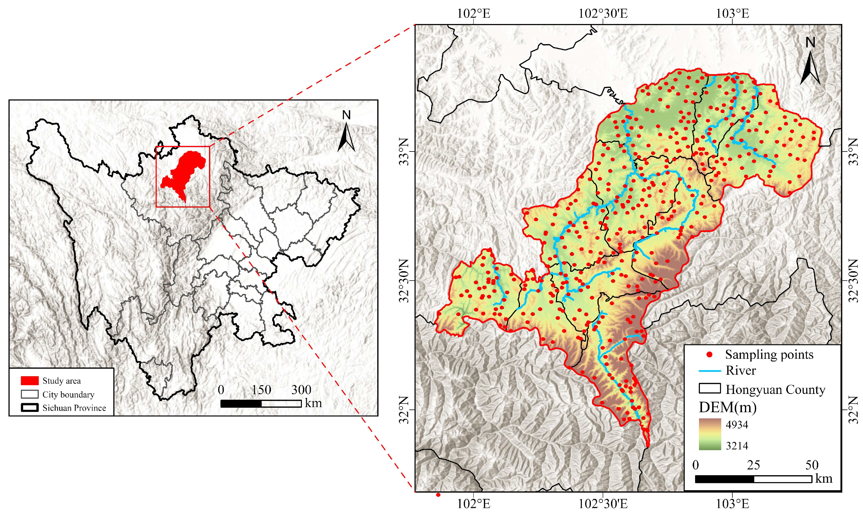
Hongyuan County is situated in the northwest of the Aba Tibetan and Qiang Autonomous Prefectures, Sichuan Province (ranging from 31°50′ to 33°22′ N latitude and 101°51′ to 103°23′ E longitude). It is located on the eastern margin of the Qinghai–Tibet Plateau, the county exhibits a typical hilly plateau landform (Figure 2), with elevations ranging from 3210 m to 4875 m and an average of approximately 3600 m. Slopes across the region are mostly between 8° and 22°. This county is a crucial water source and recharge area for the two major river basins, the Yangtze and Yellow River Basins. The core watershed, Chazhen Liangzi, covers a large part of the county. It is one of China’s key water conservation areas and forms part of the Ruo’ergai Wetland National Nature Reserve. The region has a continental alpine cold-temperate monsoon climate, with an average annual temperature of 1.4 °C, averaging about –10.3 °C in the coldest month (January) and around 10.9 °C in the warmest month (July), and an annual precipitation of about 750 mm, most of which falls from May to October. The combination of cold and humid climatic conditions with large areas of alpine meadows, swamps, and peat wetlands endows the area with large water storage and regulation capabilities. The county has a low population density, with most residents concentrated in towns such as Qiongxi, Sedi, and Waqie. The region is rich in grassland resources, which cover a total area of 504,247 hectares, accounting for 92.4% of the county’s land (according to data from the third national land survey in 2020). Alpine meadows are the dominant type; other types include swampy and shrub meadows.

2.3. Data Sources and Processing

The data encompassed remote sensing imagery data, ground measurements, soil data, and meteorological data. For remote sensing image processing, atmospheric correction, cloud masking, pansharpening, and image registration were uniformly applied. A convolutional neural network (CNN) was used to generate training data by downsampling Landsat 8 panchromatic and multispectral images by a factor of two, and a residual network (ResNet) was used to construct a fusion model, which was then used to generate high-resolution imagery of the study area. The model was trained for 100 iterations using the Adam optimizer with an initial learning rate of 10−4, which was halved every 10,000 iterations. We used 46 scenes to determine the fraction of photosynthetically active radiation (FPAR) throughout the year. Dynamic habitat indices (DHIcum, DHImin, and DHIsea) were calculated. A stratified random sampling method based on grassland type and geographic distribution was adopted to establish 435 sample plots (30 m × 30 m) to obtain ground measurements. A five-point sampling method was used to establish 1 m × 1 m quadrats. After preprocessing the measured data in ArcGIS 10.8, an RF model was applied to invert them in conjunction with the remote sensing imagery. Meteorological data were spatially interpolated using ANUSPLIN software. All datasets were resampled to a uniform 15 m spatial resolution UTM grid based on the WGS84 datum and UTM Zone 48N. Non-grassland areas including water bodies, snow cover, built-up surfaces, and bare land were masked using grassland patch data from China’s Third National Land Survey. Continuous variables (e.g., meteorological and soil data) were resampled using bilinear interpolation to maintain smoothness, while categorical data were processed using the nearest-neighbor method to preserve original values. NoData areas were uniformly assigned a value of −9999 and excluded from subsequent analysis. The data description is listed in Table 1.

2.4. Research Methods

2.4.1. Evaluation Index Screening

This study constructed an initial set of grassland classification indices (Table 2) based on those in the Regulations for Grassland Classification and Grading. These data were supplemented with regional indices of the study area [24,25] and high-frequency indices from the literature [26,27,28,29]. Initially, the XGBoost method was used to identify key indices influencing grassland classes. Subsequently, SHAP values (with 95% confidence intervals derived via Bootstrap resampling) were employed to rank the most influential indicators, followed by a collinearity analysis to eliminate those with redundant evaluation content.
The XGBoost algorithm generates a tree in each iteration and fits the residuals of the predicted values from the previous iteration by learning a new function. Based on the generated trees, new trees are trained, which retain more information from the objective function, improving the model’s training speed [30,31,32]. We used a dataset D = { ( x i , y i ) : i = 1,2 . . . , n , x i R p , y i R } , where n represents the number of samples, and J denotes the number of sample features. There are k ( k = 1,2 , , K ) regression trees, with x i and y i representing the feature vector and the target value at point i, respectively. The model can be expressed as:
ŷ i = k = 1 K f k ( x i ) , f k F
where ŷ i represents the model’s predicted result for the i-th sample, f k denotes the classification function of the k-th weak decision tree, F is the set of all possible decision trees, and f k ( x i ) indicates the score of the i-th sample in the k-th tree.
The objective function of the XGBoost algorithm consists of a loss function and a regularization term. The objective function is minimized using iteration. For example, in the s-th iteration, the expression for the objective function after iteration is as follows:
O J B ( s ) = i = 1 n L y i , y ^ ( s 1 ) + η f s ( x i ) + Ω ( f s )
where O J B ( s ) represents the objective function in the s-th iteration. The first term, L y i , y ^ ( s 1 ) + η f s ( x i ) , is the loss function of the model, where y ^ ( s 1 ) is the predicted result from the (s−1)-th iteration, f s ( x i ) is the newly trained tree model in the s-th iteration, and η is the shrinkage coefficient of the newly generated tree model, with η∈[0, 1]. This coefficient is used to reduce the impact of the newly generated tree on the model to prevent overfitting. The second term, Ω ( f s ) is the regularization term, which is calculated as follows:
Ω ( f ) = γ T + 1 2 λ w 2
where T represents the number of leaves in each decision tree, w denotes the leaf weights, and γ and λ are coefficients. When a new decision tree is generated, XGBoost determines whether to prune a node based on whether the objective function value decreases after node splitting. Grid search cross-validation (GridSearchCV) was employed for hyperparameter optimization to obtain the optimal combination of hyperparameters.

2.4.2. Construction of the Evaluation Model

  • Spatial block cross-validation and Synthetic Minority Over-sampling Technique
Due to potential imbalances in the number of sample points across different grassland classes, machine learning methods may suffer from overfitting or underfitting, failing to reflect the true distribution of grassland classes. This study employed a 5-fold buffer cross-validation (Buffer CV) approach, partitioning the study area into five non-overlapping geographical blocks with a 5 km radius. In each fold, one block was designated as the validation set, and the remaining four constituted the training set. To address class imbalance, the Synthetic Minority Over-sampling Technique (SMOTE) was applied exclusively to the training data while the validation set was strictly withheld from the synthesis process to prevent data leakage [33].
  • Histogram Gradient Boosting
The gradient boosting machine (GBM) constructs a strong model by serially training multiple weak learners (typically decision trees) to correct errors made by the previous one. HistGradientBoosting represents a modern, high-performance implementation of GBM, with its core innovation being the use of histograms to accelerate the construction of decision trees. This approach significantly improves training speed and scalability while maintaining GBM’s high accuracy advantages [34]. The methodological steps are as follows:
  • Initialization:
It begins with the initial predicted values for all samples. For classification problems, the initial model F 0 ( x ) uses the prior probability (in log-odds form) of each sample belonging to every class.
2.
Iterative Tree Construction:
a. Calculate the Negative Gradient (Pseudo-Residuals): For each sample i, compute the negative gradient of the current model F m 1 ( x ) (i.e., the negative gradient of the loss function). This gradient indicates the direction and magnitude of the error in the current prediction. The formula is as follows:
r i m = L ( y i , F ( x i ) ) F ( x i ) F ( x ) = F m 1 ( x )
b. Fit a Weak Learner: Train a new decision tree h m ( x ) , where the target is the pseudo-residuals calculated in the previous step. This tree learns how to correct the errors of the current model.
c. Line Search for the Weight: Determine an optimal step size γ m to scale the contribution of this tree to minimize the loss function. The formula is as follows:
γ m = arg min γ i = 1 n L ( y i , F m 1 ( x i ) + γ h m ( x i ) )
d. Update the Model: Incorporate the new tree into the ensemble model.
F m ( x ) = F m 1 ( x ) + ν γ m h m ( x )
where ν represents the learning rate, which controls the magnitude of the tree’s contribution and prevents overfitting.
3.
Obtain the Final Model:
F m ( x ) = F 0 ( x ) + ν m = 1 M γ m h m ( x )
where F m ( x ) denotes the final strong learner obtained after M iterations; F 0 ( x ) is the initial model; ν is the learning rate, which helps prevent overfitting by scaling down the contribution of the trees; h m ( x ) represents the weak learner (i.e., a decision tree) generated during the m-th iteration; ν m = 1 M γ m is the summation of all trees from the 1st to the M-th round of iterations.
  • Light Gradient Boosting Machine
The LightGBM is an open-source gradient boosting framework developed by Microsoft. Its core objective is to significantly enhance training speed and reduce memory consumption while maintaining high accuracy. Its formulaic approach can be summarized as a classic gradient boosting framework + (gradient-based one-sided sampling (GOSS)) + (exclusive feature bundling (EFB)). It employs GOSS for efficient sampling in the row (sample) dimension and utilizes EFB for intelligent compression in the column (feature) dimension. These two engines work in tandem, providing LightGBM with notable advantages over other gradient boosting algorithms for handling large-scale, high-dimensional data, including extremely fast training speed, minimal memory consumption, and improved accuracy [35].
  • Random Forest
Unlike gradient boosting models, RF is an ensemble learning method focusing on collective decision-making rather than step-by-step correction. It utilizes dual randomness to prevent overfitting, is robust to data noise and missing values, and can deliver reliable results without complex parameter tuning. The core strengths of the RF model for grassland classification are its high robustness, rapid training speed, and high model interpretability.
  • Hyperparameter Optimization and Accuracy Validation
Hyperparameter optimization was performed using RandomizedSearchCV (scikit-learn 1.3) with the following settings: n_iter = 80, cv = 5, n_jobs = −1, and random_state = 42. The parameter search space encompassed learning_rate, max_depth, n_estimators, and max_iter.
Model performance was comprehensively evaluated using six metrics: overall accuracy, precision, recall, weighted F1-score, along with per-class F1-scores and AUC (Area Under the ROC Curve) values.

3. Results

3.1. Image Fusion Results

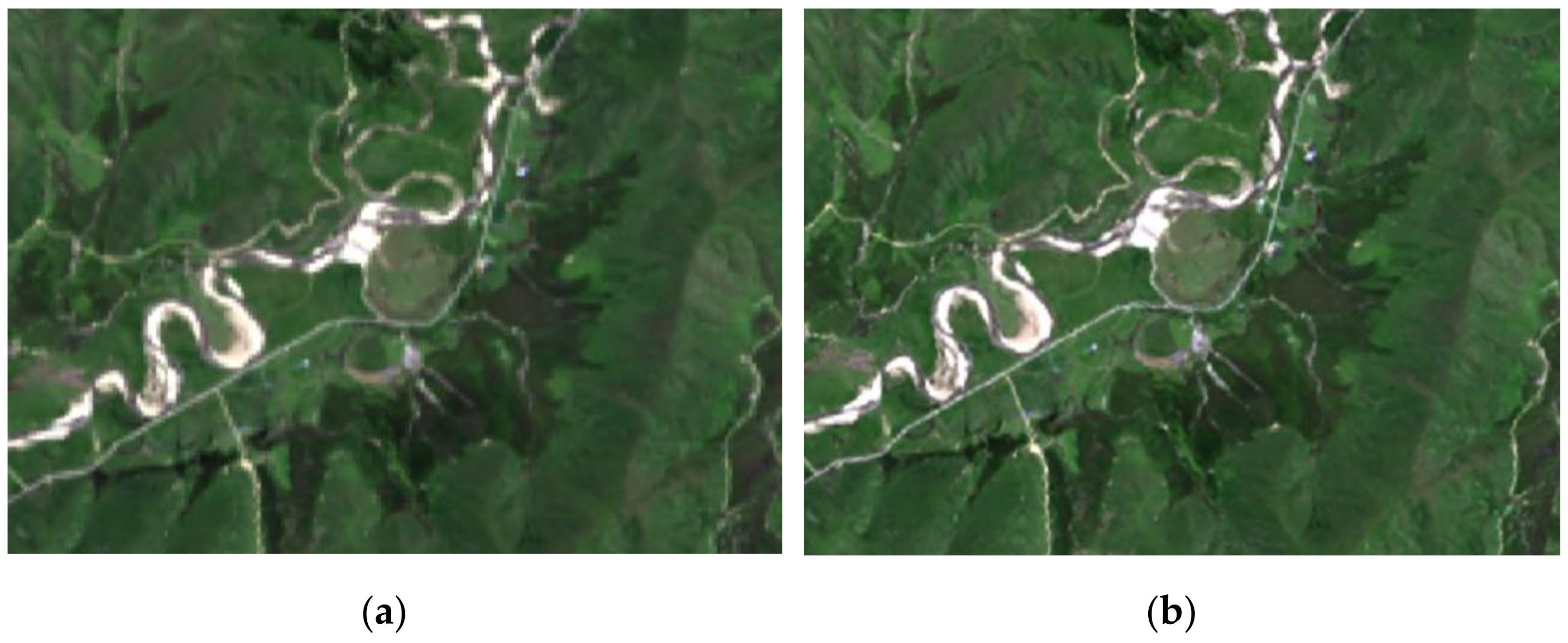
The fused images exhibit significantly better clarity and more details than the original images (Figure 3). A comparison was conducted between the proposed method and the Gram-Schmidt (GS) method. The root mean square error (RMSE) and peak signal-to-noise ratio (PSNR) were selected as evaluation metrics. The results are presented in Table 3.
The RMSE values of the GS algorithm ranged from 0.08 to 0.41, with an average of 0.2026. In contrast, the RMSE values of the proposed method ranged from 0.02 to 0.09 across different benchmarks, with an average of 0.0524, which was 74.13% lower than that of the GS algorithm. The PSNR values of the GS algorithm ranged from 21.52 to 37.09, with an average of 19.86, whereas those of the proposed method ranged from 26.7 to 43.41, with an average of 25.73; this value was 29.57% higher than that of the GS algorithm. These results indicate that the proposed method exhibits lower and more stable error rates across all benchmarks.

3.2. Results of Indicator Screening

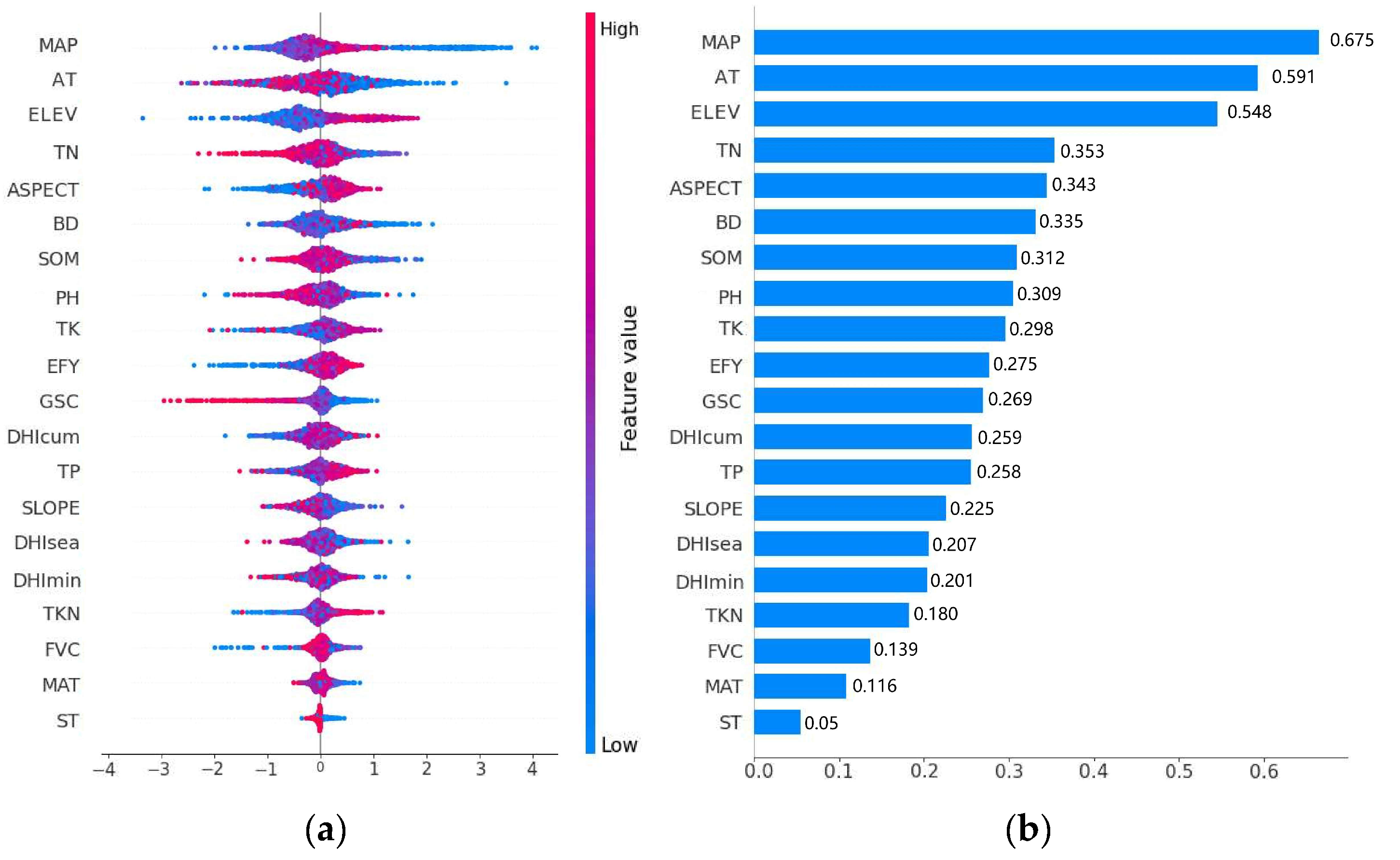
The features were ranked by importance based on their SHAP values is shown in Figure 4. The mean annual precipitation (MAP) ranked first in feature importance, followed by >0 °C Accumulated Temperature (AT) and elevation (ELEV). Elevation affects precipitation and temperature. Therefore, it can be inferred that hydrothermal conditions are the primary factor influencing grassland classes in this region. Soil Texture (ST), mean average temperature (MAT), and fractional vegetation cover (FVC) had low feature importance, suggesting that the impact of ST on grassland classes was minor under the combined influence of hydrothermal factors, microenvironmental modifications, and plant adaptive strategies. Although MAT and AT are temperature indicators, their importance differed significantly, possibly because MAT, a static average, does not reflect the dynamic thermal conditions during the growing season. The low feature importance of FVC may be attributed to the fact that it does not describe the vegetation type (e.g., the ratio of edible forage to toxic weeds), plant height, or vertical biomass distribution, although it represents grassland vegetation cover, limiting its influence on grassland classes.
The top 15 factors ranked by importance were imported into SPSS 4.0 for collinearity analysis. Five exhibited significant collinearity (variance inflation factor (VIF > 5, Table 4): MAP, Soil Organic Matter (SOM), Soil Bulk Density (BD), ELEV and Total Nitrogen (TN). These indicators were sequentially removed starting from the one with the highest VIF value. After eliminating TN and ELEV, the VIF values of MAP and SOM fell below 5, leaving only BD with a VIF greater than 5. After removing BD, the VIF values of the remaining 12 indicators were below 5, indicating no significant collinearity (Table 5). The reason may be that TN, ELEV and BD represent ecological coupling nodes at three levels: nutrient cycling, terrain-driven, and physical integration. Removing them deconstructs the ecological chain of climate, terrain, organic matter, soil structure, and nitrogen so that the remaining factors become independent.
The final indicators, ranked from highest to lowest importance, were MAP, AT, ASPECT, SOM, potential of Hydrogen (PH), Total Potassium (TK), Edible Forage Yield (EFY), surface soil gravel content (GSC), cumulative annual productivity (DHIcum), Total Phosphorus (TP), SLOPE, and seasonal variation in productivity (DHIsea). The first and second rankings of MAP and AT, which are climatic factors, highlight the significant influence of hydrothermal conditions on alpine grassland ecosystems. ASPECT, which ranked third, surpassed some soil indicators, indicating that terrain significantly influences the spatial differentiation of grassland types and quality due to solar radiation. Among the soil factors, the chemical indicators SOM, PH, TK, and TP ranked fourth, fifth, sixth, and tenth, respectively, reflecting the significant constraints of soil fertility and chemical environment on grassland productivity. The physical soil factor GSC ranked eighth, possibly because gravel cover influences grassland growth conditions in the unique freeze–thaw cycle environment of alpine regions by affecting soil insulation and moisture retention, reducing water evaporation, and regulating surface runoff. Among the vegetation-related factors, EFY, DHIcum, and DHIsea ranked seventh, ninth, and twelfth, respectively, demonstrating that vegetation, the output of grasslands, is directly driven and substantially constrained by environmental factors, such as hydrothermal conditions, terrain, and soil.
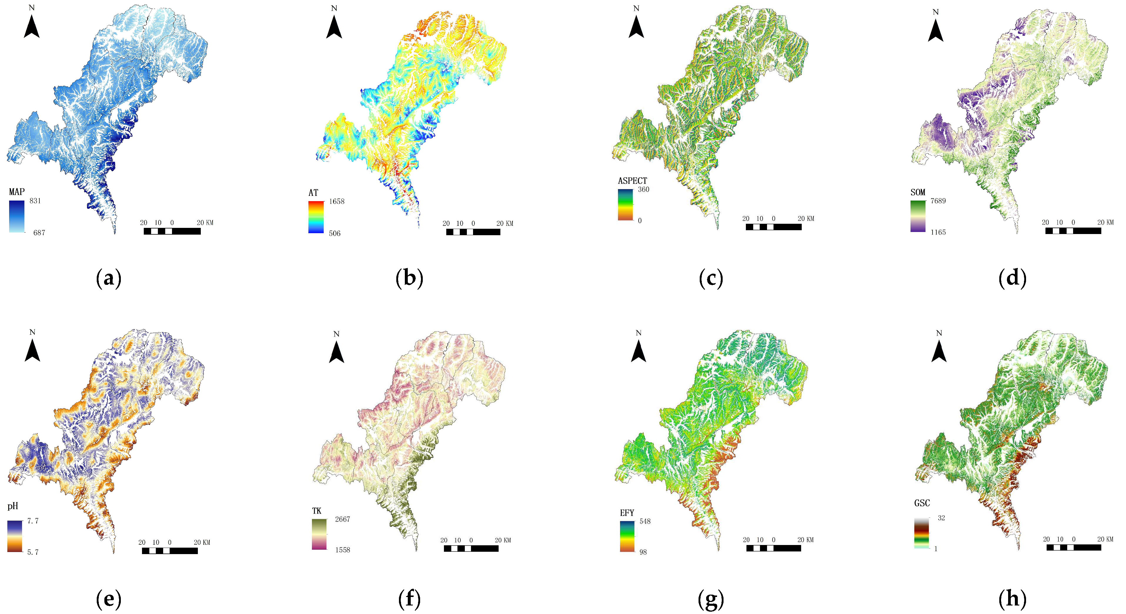
This ranking result reveals that climate factors had the largest influence on alpine grassland classes, followed by terrain, soil, and vegetation factors. Hydrothermal conditions determine the basic pattern, while terrain factors create a secondary differentiation through local habitat reconstruction. Soil properties provide materials and nutrients, and vegetation parameters reflect the functional output of the system. This sequence objectively reflects the factor weights for the grassland classes. Notably, although ELEV was excluded due to high collinearity, its ecological functions are considered by slope, aspect, and hydrothermal factors. However, the importance of slope differed significantly from that of other factors, possibly because slope primarily influences the transport and distribution of surface materials (water, soil, and nutrients) through gravity but does not affect hydrothermal conditions like aspect. Its effects are relatively indirect and complex; thus, some of its functions can be substituted by soil and moisture factors. This result reveals that energy distribution (aspect) has a larger influence than material distribution (slope) on alpine grassland systems. The spatial distribution of the indicators is shown in Figure 5.

3.3. Grassland Class Evaluation

Evaluation models were constructed using XGBoost, HistGradientBoosting, LightGBM, and RF to assess the grassland classification. A total of 5630 sample points were selected for model training, and 2413 sample points were used to validate model accuracy. The optimal models were obtained after training and parameter tuning. The evaluation indicators were the inputs, and the grassland classes were the outputs. The model parameters are listed in Table 6. The accuracy validation results of each model are presented in Table 7. The grassland quality was classified into three levels (Classes 1–3), where Class 1 denotes the highest quality grassland and Class 3 represents the lowest quality.
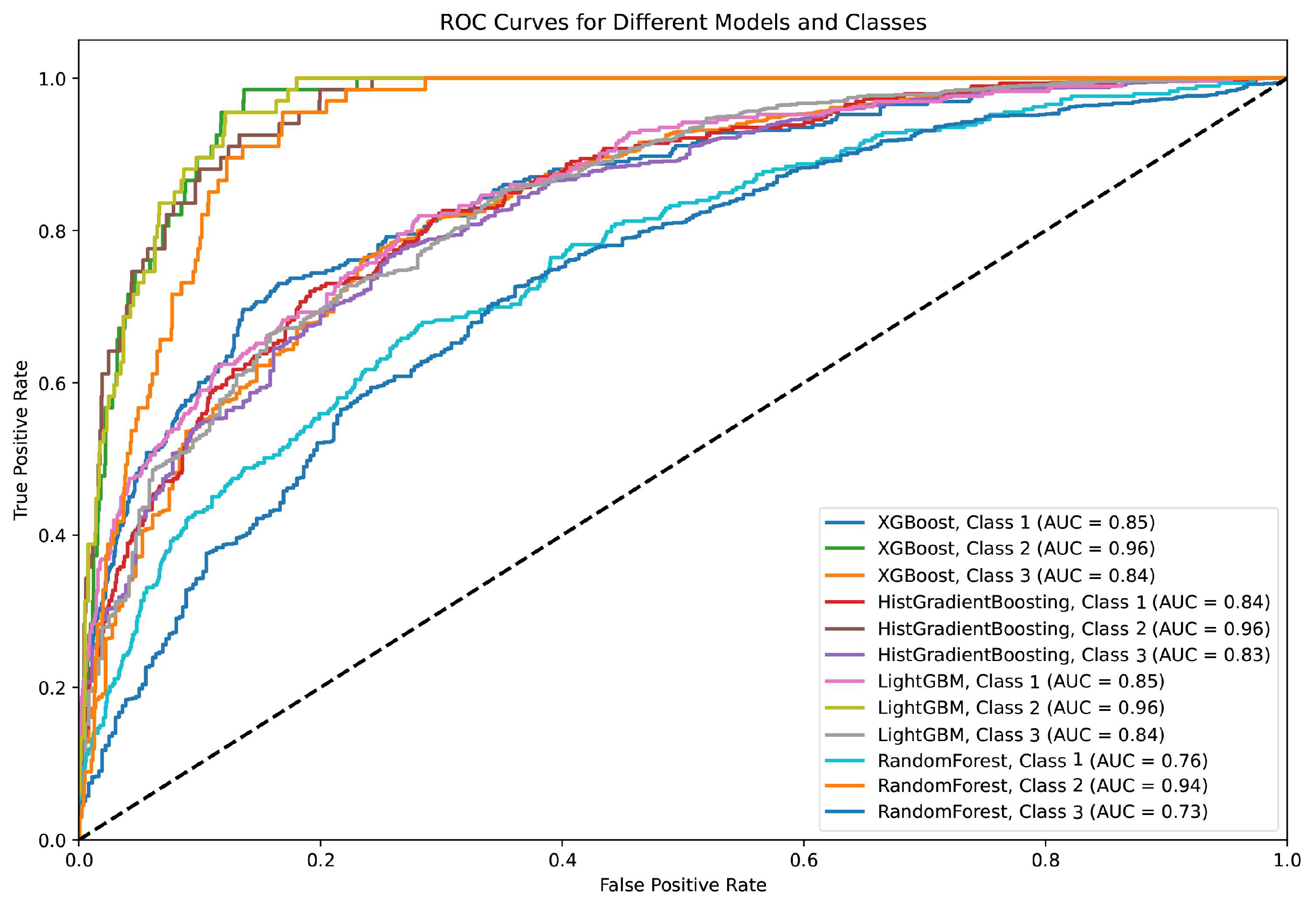
The models shared the same ranking order across Accuracy, Precision, Recall, and weighted F1-Score: XGBoost > LightGBM > HistGradientBoosting > RF. The accuracy rates of XGBoost, LightGBM, and HistGradientBoosting exceeded 0.8, whereas RF had an accuracy rate of 0.64. To further evaluate the prediction accuracy of the models across different grassland classes, we performed a class-wise analysis of F1-scores and AUC. In terms of per-class F1-scores (Table 6), all models exhibited a decrease of over 0.3 in Classes 1 and 3 compared to Class 2, indicating that most misclassifications occurred between Classes 1 and 3. This may be attributed to the imbalanced sample distribution across grassland classes (Class 1: 293 samples; Class 2: 1249 samples; Class 3: 67 samples). The class-wise AUC results showed that HistGradientBoosting, XGBoost, and LightGBM across all grassland classes exceeded 0.8, whereas RF had AUC values less than 0.8 for grassland classes 1 and 3 (Figure 6). Thus, RF exhibited the lowest performance, whereas XGBoost, LightGBM, and HistGradientBoosting showed similar results. The XGBoost model demonstrated the highest accuracy, stability, and predictive capability, making it suitable for classifying grasslands.
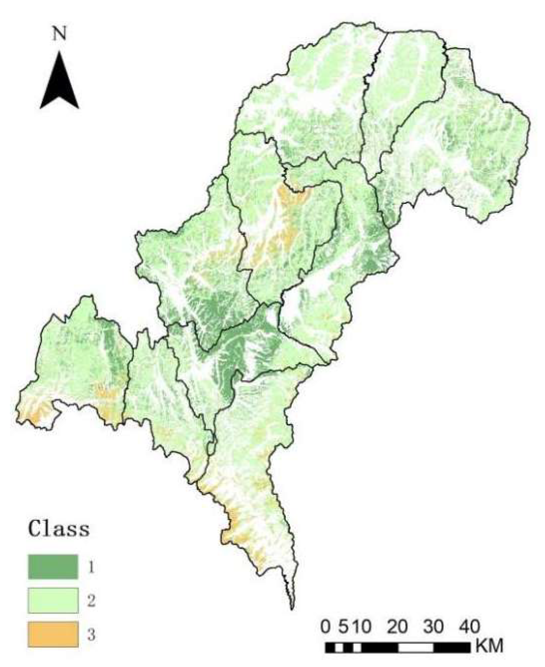
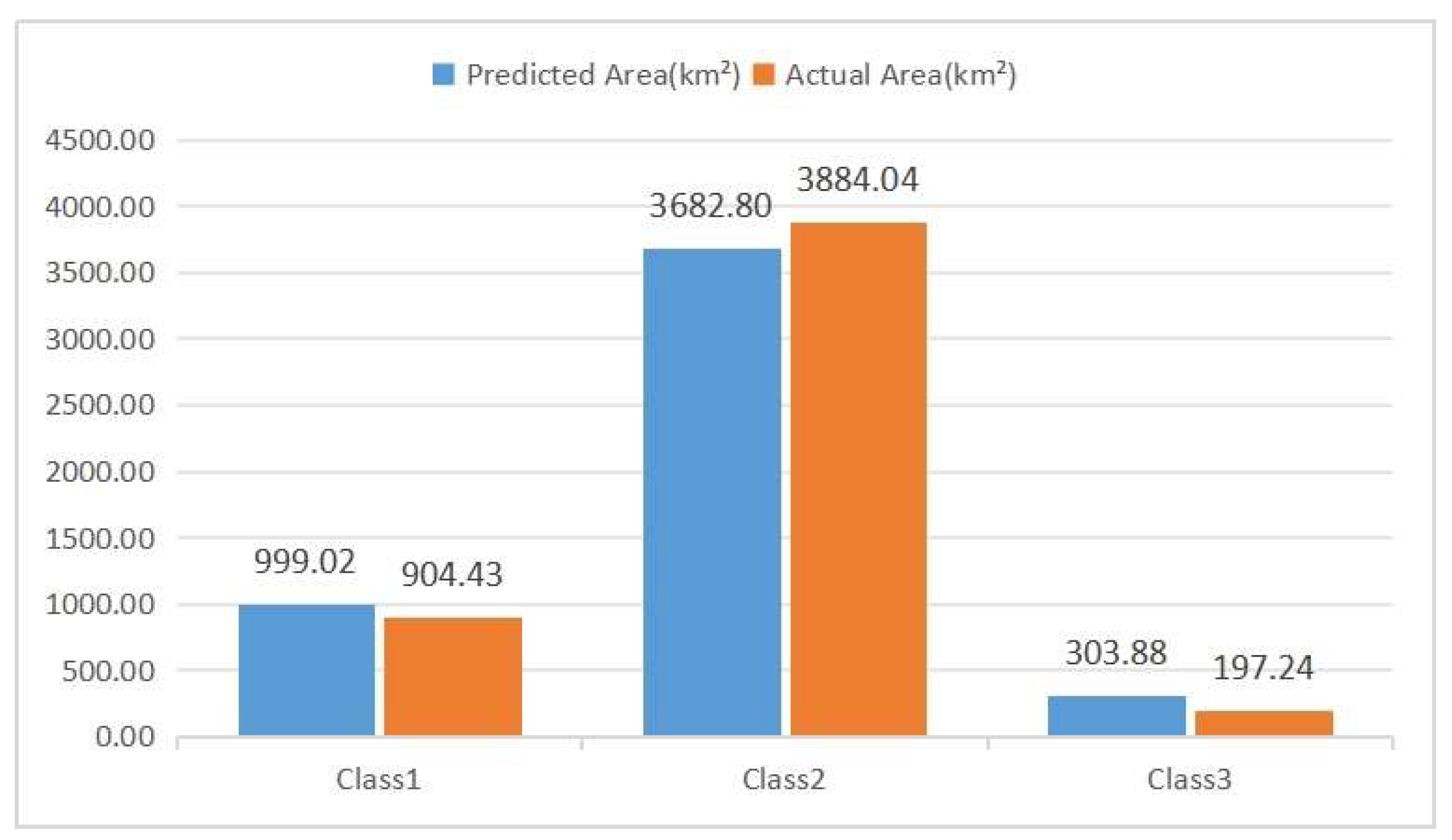
The model predicted three grassland classes in Hongyuan County (Figure 7). Class 1 accounted for 22.04% (95% CI: 20.81–23.28%), covering 999.02 km2 primarily in the southern part of Anqu Town, Longri Town, the eastern part of Chaerma Township, and the central part of Kemu Township. Class 2 comprised 71.67% (95% CI: 70.15–73.19%) of the grasslands, with an area of 3682.80 km2. It was widely distributed across the county, predominantly in Waqie Town, Sedi Town, Maiwa Township, Amu Township, Jiangrong Township, the southern part of Kemu Township, the western part of Chaerma Township, the northern part of Shuajingsi Town, and the northwestern part of Qiongxi Town and Anqu Town. Class 3 accounted for 6.29% (95% CI: 5.67–6.91%), covering 303.88 km2 primarily in the central part of Qiongxi Town, the southern part of Chaerma Township, and the southern part of Shuajingsi Town.
The reasons for these results may be as follows. The southern part of Anqu Town, Longri Town, and the central part of Kemu Township have flat and open terrain, abundant water sources with good drainage, fertile soil primarily consisting of meadow soil, and a relatively mild climate, providing an ideal environment for the growth of high-quality forage grasses, resulting in the best grassland class. In contrast, the southern part of Shuajingsi Town has steep slopes with thin soil layers, low water and fertilizer retention, and high susceptibility to erosion. Additionally, large differences in elevation result in few contiguous high-quality grasslands. The southern part of Chaerma Township is located at high altitudes, where cold temperatures and strong winds result in a very short growing season and a lack of heat, limiting the growth and recovery of forage grasses. Qiongxi Town, the county seat, experiences the most concentrated and frequent human activities. Long-term, high-intensity grazing pressure, infrastructure construction, and daily production and living activities have caused severe trampling, damaging grasslands and resulting in the lowest-quality grassland class. The Class 2 grasslands, which accounted for over 70% of the total area, dominated vast hilly plateau regions, such as Waqie Town, Sedi Town, Maiwa Township, Amu Township, and Jiangrong Township. These are regions with alpine meadow ecosystems in Hongyuan County, characterized by gently rolling terrain at moderate altitudes, alpine climatic conditions, and alpine meadow soils. The relatively moderate or controlled grazing activities in these regions ensure moderate grassland productivity, resulting in the class with the largest proportion.

3.4. Validation of Evaluation Results

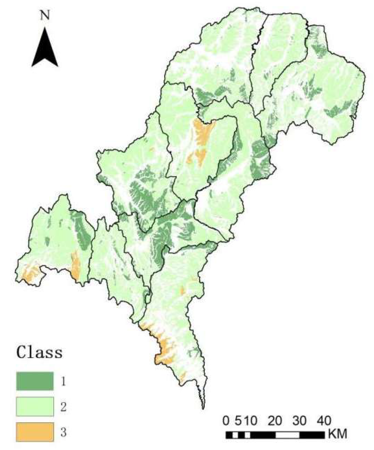
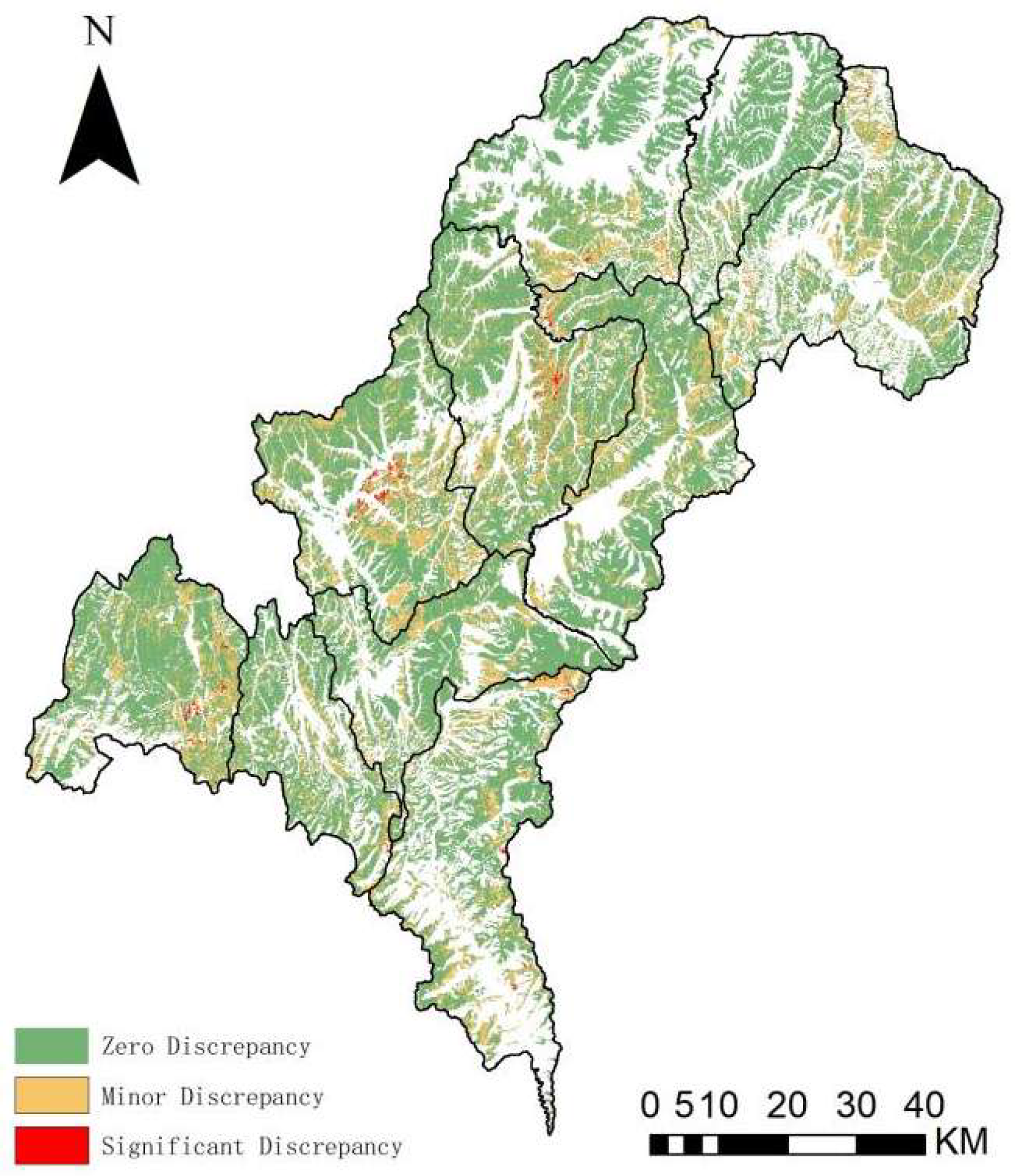
In the actual grassland classes of Hongyuan County in 2022 (Figure 8), Class 1 accounted for 18.14%, covering 904.43 km2 primarily in the central and southern parts of Anqu Town, Longri Town, the eastern part of Chaerma Township, the southern part of Waqie Town, and the central part of Kemu Township, with sporadic distributions in Sedi Town. Class 2 comprised 77.90% of the grasslands, with an area of 3884.04 km2 and was widely distributed across the county, predominantly in Waqie Town, Sedi Town, Maiwa Township, Amu Township, Jiangrong Township, the northern and southern parts of Kemu Township, the northern part of Shuajingsi Town, the western part of Chaerma Township, Qiongxi Town, and the northwestern part of Anqu Town. Class 3 accounted for 3.96%, covering 197.24 km2 primarily in the central part of Qiongxi Town, the southern part of Chaerma Township, and the southern part of Shuajingsi Town (Figure 8). A quantitative comparative evaluation of predicted versus actual grassland classes revealed high agreement for the dominant Class 2 grasslands (Kappa = 0.794), indicating the model accurately captured the spatial configuration of this primary grassland type. Classes 1 (Kappa = 0.502) and 3 (Kappa = 0.436) showed moderate consistency, with discrepancies mainly from boundary effects at class transitions and the class imbalance due to the limited sample size of Class 3 (accounting for only 3.96%). Overall, despite localized variations in non-dominant classes, the model predictions effectively reproduced the overall spatial distribution pattern of actual grassland classes. A comparison of the area proportions of the grassland classes for both classification schemes is shown in Figure 9.
To further investigate the sources of prediction errors, we analyzed discrepancies from both quantitative and spatial distribution perspectives. In terms of quantitative differences, the area proportions of each class predicted by the model (Class 1: 22.04%, Class 2: 71.67%, Class 3: 6.29%) closely matched the actual proportions (Class 1: 18.14%, Class 2: 77.90%, Class 3: 3.96%), indicating minimal quantitative discrepancy between the two sets of results (Figure 9). For spatial distribution differences, we performed a pixel-by-pixel absolute difference calculation between the model-predicted and actual grassland classes, generating a spatial distribution map of classification discrepancies (Figure 10). The results revealed that 75.82% of the total area showed perfect agreement between predicted and actual classes (absolute value = 0), while minor discrepancies were observed in 23.63% of the area. These minor discrepancies were primarily located near the Class 1 and Class 3 grassland areas in Chaerma Township, Anqu Town, Qiongxi Town, Waqie Town, and Sedi Town. This result may be attributed to differences between the model-predicted grid-based transitions and the actual patch-based hard classification, resulting in numerous discrepancies with an absolute value of 1 at the boundaries between Class 1, Class 3 and Class 2 grasslands. Areas with major discrepancies (absolute value = 2) accounted for 0.54% and were mainly concentrated in the central parts of Anqu Town and Qiongxi Town. It was attributed to the fact that these regions, which are county seats or town centers, experienced intense development and utilization or robust protection measures in certain areas, leading to outcomes that were significantly worse or better than predicted. The comparative analysis of the discrepancies demonstrates that the grassland classes were aligned closely with actual conditions in most areas align, indicating that the proposed grassland class evaluation model is reasonable.

4. Discussion

This study utilized multi-source remote sensing data and machine learning methods for grassland classification in the water conservation area of the Qinghai–Tibet Plateau, using Hongyuan County as a case study. Unlike traditional evaluation systems that rely on expert experience and linear weighting, this approach demonstrated significant advantages in terms of data accuracy, objectivity in indicator selection, and model performance. Based on the findings of this study and the literature, the following was observed. This study aligns with recent trends in grassland remote sensing monitoring, with distinct characteristics. In contrast to the studies by Li Xia, Zhang Zihui [20], and others, which focused on biomass estimation, this study applied machine learning to perform comprehensive grassland classification, integrating multidimensional indicators like climate, topography, soil, and vegetation. In contrast to Yihan Ma’s [22] semi-supervised clustering approach, this study systematically compared gradient boosting algorithms and found that XGBoost was superior in classifying alpine grasslands. The indicators were consistent with those selected by Wen Liu [36], Ma Fulin [37], and others in studies on grassland growth attribution on the Qinghai–Tibet Plateau. Their findings confirm that in high-altitude regions, MAP and AT directly determine the length of the growing season and the intensity of water stress, thereby establishing the fundamental pattern of grassland productivity. The dominant role of climate is not isolated but is realized through complex interactions with topography and soil. For instance, aspect creates local microclimates by redistributing solar radiation. South-facing slopes receive more radiation, resulting in higher soil temperatures and stronger evaporation, which can exacerbate physiological drought to some extent; whereas north-facing slopes are cooler and more humid. This topography-mediated hydrothermal differentiation directly influences soil development processes (such as organic matter decomposition rates and pedogenesis) and physical properties (such as texture and soil depth). For example, on moist, shaded slopes, conditions are more conducive to the accumulation of fine particles and organic matter, forming soils with better water and nutrient retention capabilities; on dry, sunny slopes, soils are often thinner and higher in gravel content. Thus, climate shapes the microenvironment through topography and ultimately couples with soil attributes to jointly determine grassland vegetation growth status and the spatial differentiation of grassland classes. XGBoost performed best for classifying alpine grasslands in Hongyuan County (with an accuracy of 0.829), whereas RF had the lowest performance (with an accuracy of 0.644). From the perspective of the alignment between algorithmic characteristics and our data features, Boosting algorithms effectively learn subtle, nonlinear decision boundaries from complex features by sequentially building weak learners and focusing on previously misclassified samples. In this study, the relationship between grassland classes and environmental factors likely exhibits such complex nonlinear patterns. Furthermore, XGBoost’s built-in regularization terms provide better protection against overfitting, resulting in stronger robustness and higher final accuracy. This finding aligns with the results reported by Liu Huiwen [38], confirming the effectiveness of our method in the Qinghai–Tibet Plateau region. However, in other regions, such as in the study on aboveground biomass (AGB) estimation in temperate grasslands in Inner Mongolia [39], where stepwise linear regression outperformed complex machine learning algorithms. These seemingly contradictory results underscore the high dependency of machine learning model performance on environmental conditions, data scale, and prediction targets of the study area. Therefore, it is essential to consider the regional applicability of the model and conduct thorough localized validation and comparison when applying machine learning to grassland resource evaluation.
This study performed a comprehensive quality classification of alpine grasslands in the water conservation area of the Qinghai–Tibet Plateau but did not address biomass, leaf area index, or vegetation type classification. The results indicate the quality characteristics of grasslands as natural resources. This study employed a CNN deep learning method to fuse Landsat panchromatic and multispectral images, generating a 15 m high-resolution temporal dataset (the RMSE was 74.13% lower than for the GS method), providing an effective high-precision solution for regions lacking hyperspectral data. The XGBoost algorithm was used to quantify feature importance while ensuring the relative independence of indicators through collinearity analysis, avoiding the subjectivity of the Delphi method and the assumption of linearity in PCA. The results showed that hydrothermal factors (MAP and AT) and topographic factors (ASPECT) had higher importance than traditionally emphasized soil indicators, revealing that climate factors had the largest influence on alpine grassland classes, followed by terrain, soil, and vegetation factors. A comparison of four machine learning algorithms demonstrated that XGBoost achieved the highest accuracy (0.829), indicating that machine learning algorithms can capture the complex nonlinear relationships between alpine grassland classes and environmental factors, addressing the subjectivity issues inherent in linear weighting methods.
Meanwhile, this study has several limitations that also indicate directions for future research: (1) Temporal scale limitation: The analysis primarily relied on single-year (2022) data, which prevented capturing interannual dynamics of grassland classes, particularly their responses to climate fluctuations and extreme events. (2) Seasonal sampling limitation: Indicator extraction depended entirely on growing-season data, potentially inadequately representing grassland conditions during the non-growing season and thus limiting a comprehensive annual evaluation. (3) Data resampling artifacts: The standardization of original data from diverse sources and spatial resolutions to a common grid might have introduced loss of spatial detail or potential smoothing effects. (4) Lack of external regional validation: The model’s generalization capacity remains untested beyond Hongyuan County, requiring further assessment of its broader applicability. (5) Insufficient analysis of human activities: Due to limited availability of human activity and protected area vector data, we could not conduct quantitative spatial overlay analyses in regions with major discrepancies, somewhat restricting more precise verification of error mechanisms. Future studies should prioritize collecting and integrating multi-source data, such as socio-economic statistics, land use planning, and ecological conservation policies, to develop a more comprehensive analytical framework for accurately quantifying the impacts of human activities on grassland class assessment.

5. Conclusions

This study successfully developed and validated an integrated grassland classification framework that combines multi-source remote sensing data and machine learning. The main conclusions are summarized as follows:
(1)
Regarding data processing, a CNN-based deep learning model was employed to fuse Landsat panchromatic and multispectral images, producing a 15 m high-resolution temporal dataset. Quantitative evaluation demonstrated that the fusion quality achieved a 74.13% reduction in RMSE (to 0.0524) and a 29.57% increase in PSNR compared to the GS fusion method. This approach effectively mitigated the mixed-pixel issue in medium-resolution remote sensing over plateau regions, providing a reliable data foundation for accurate inversion of vegetation parameters such as FVC.
(2)
In terms of indicator screening, this study applied XGBoost combined with collinearity analysis (VIF < 5) to quantitatively identify hydrothermal conditions (MAP and AT) as the dominant drivers of alpine grassland class differentiation. Aspect, functioning as an energy regulator, demonstrated greater importance than most soil and vegetation indicators. This finding enhances our understanding insight into the formation mechanisms of alpine grassland ecosystems.
(3)
A systematic comparison demonstrated that XGBoost achieved optimal classification performance, with an overall accuracy of 0.829. A pixel-by-pixel absolute difference analysis between the predicted and actual grassland classes revealed perfect agreement in 75.82% of the area, minor discrepancies in 23.63%, and major discrepancies in only 0.54%. Grasslands of class 2 were dominant (71.67%), while Class 1 and Class 3 grasslands were mainly distributed in river valleys with favorable hydrothermal conditions and in alpine or urban areas subject to human disturbance or harsh natural conditions, respectively.
(4)
This framework provides an objective and efficient monitoring approach for administrative departments, including strict protection for high-quality grasslands (Class 1), carrying capacity-based grazing for widespread grasslands (Class 2), and precision restoration for degraded grasslands (Class 3), for instance, planting drought-resistant species on south-facing slopes. By closely linking grassland conditions with dominant climatic factors, this method offers a replicable scientific tool for establishing dynamic early-warning systems and adaptive management strategies in response to future climate change.
(5)
Future research efforts should focus on the following directions: applying the framework to multi-year time-series data to dynamically monitor grassland responses to climate change and human activities; integrating SAR data to compensate for optical remote sensing gaps during cloudy and rainy seasons in the plateau; and conducting independent validation and transferability studies in adjacent counties to enhance model generalization.

Author Contributions

Conceptualization, K.Y. and Y.H.; methodology, K.Y. and L.W.; software, R.Z. and T.W.; validation, K.Y. and F.Y.; formal analysis, K.Y.; investigation, K.Y.; resources, T.W.; data curation, F.Y.; writing—original draft preparation, K.Y.; writing—review and editing, K.Y. and R.Z.; visualization, K.Y.; supervision, X.H.; project administration, L.Z.; funding acquisition, Y.H. All authors have read and agreed to the published version of the manuscript.

Funding

Project Name: Remote Sensing Big Data Platform for Land Consolidation and Ecological Restoration in Sichuan Province and Industrial Application Demonstration. Grant Number: 87-Y50G29-9001-22/23.

Institutional Review Board Statement

Not applicable.

Data Availability Statement

The data presented in this study are available in this article.

Conflicts of Interest

The authors declare no conflicts of interest.

References

  1. Xie, G.D.; Zhang, Y.L.; Lu, C.X.; Xie, G.D.; Zhang, Y.L.; Lu, C.X.; Zheng, D.; Cheng, S.K. Service value of natural grassland ecosystems in China. J. Nat. Resour. 2001, 1, 47–53. [Google Scholar]
  2. Liu, H.; Hou, L.; Kang, N.; Nan, Z.; Huang, J. A meta-regression analysis of the economic value of grassland ecosystem services in China. Ecol. Indic. 2022, 138, 108793. [Google Scholar] [CrossRef]
  3. Guan, Z.H.; Liu, G.H.; He, J.S. Research Status and Development Trends of Grassland Protection Technologies: A Literature Analysis. Pratacultural Sci. 2020, 37, 703–717. [Google Scholar]
  4. Bardgett, R.D.; Bullock, J.M.; Lavorel, S.; Manning, P.; Schaffner, U.; Ostle, N.; Chomel, M.; Durigan, G.; Fry, E.L.; Johnson, D.; et al. Combatting global grassland degradation. Nat. Rev. Earth Environ. 2021, 2, 720–735. [Google Scholar] [CrossRef]
  5. Xie, G.D.; Lu, C.X.; Xiao, Y.; Zheng, D. Valuation of alpine grassland ecosystem services on the Tibetan Plateau. J. Mt. Sci. 2003, 21, 50–55. [Google Scholar]
  6. Yao, T.D. Investigation of Water-Ecology-Human Activities Reveals the Imbalance of the Asian Water Tower and Its Potential Risks. Chin. Sci. Bull. 2019, 64, 2761–2762. [Google Scholar]
  7. Fu, B.J.; Ouyang, Z.Y.; Shi, P.; Fan, J.; Wang, X.D.; Zheng, H.; Zhao, W.W.; Wu, F. Current Condition and Protection Strategies of Qinghai-Tibet Plateau Ecological Security Barrier. Bull. Chin. Acad. Sci. 2021, 36, 1298–1306. [Google Scholar]
  8. Wang, Y.; Lv, W.; Xue, K.; Wang, S.; Zhang, L.; Hu, R.; Zeng, H.; Xu, X.; Li, Y.; Jiang, L.; et al. Grassland changes and adaptive management on the Qinghai–Tibetan Plateau. Nat. Rev. Earth Environ. 2022, 3, 668–683. [Google Scholar] [CrossRef]
  9. Adar, S.; Sternberg, M.; Argaman, E.; Henkin, Z.; Dovrat, G.; Zaady, E.; Paz-Kagan, T. Testing a novel pasture quality index using remote sensing tools in semiarid and Mediterranean grasslands. Agric. Ecosyst. Environ. 2023, 357, 108674. [Google Scholar] [CrossRef]
  10. Blaix, C.; Alard, D.; Chabrerie, O.; Diquélou, S.; Dutoit, T.; Fontès, H.; Lemauviel-Lavenant, S.; Loucougaray, G.; Michelot-Antalik, A.; Bonis, A. Plant evenness improves forage mineral content in semi-natural grasslands. Agric. Ecosyst. Environ. 2025, 387, 109622. [Google Scholar] [CrossRef]
  11. Wang, Z.; Zhang, Y.; Yang, Y.; Zhou, W.; Gang, C.; Zhang, Y.; Li, J.; An, R.; Wang, K.; Odeh, I.; et al. Quantitative assess the driving forces on the grassland degradation in the Qinghai–Tibet Plateau, in China. Ecol. Inform. 2016, 33, 32–44. [Google Scholar] [CrossRef]
  12. Wang, S.; Jia, L.; Cai, L.; Wang, Y.; Zhan, T.; Huang, A.; Fan, D. Assessment of Grassland Degradation on the Tibetan Plateau Based on Multi-Source Data. Remote Sens. 2022, 14, 6011. [Google Scholar] [CrossRef]
  13. Wachendorf, M.; Fricke, T.; Möckel, T. Remote sensing as a tool to assess botanical composition, structure, quantity and quality of temperate grasslands. Grass Forage Sci. 2018, 73, 1–14. [Google Scholar] [CrossRef]
  14. Zhou, Y.; Liu, T.; Batelaan, O.; Duan, L.; Wang, Y.; Li, X.; Li, M. Spatiotemporal fusion of multi-source remote sensing data for estimating aboveground biomass of grassland. Ecol. Indic. 2023, 146, 109892. [Google Scholar] [CrossRef]
  15. Wang, W.; Ma, Q.; Huang, J.; Feng, Q.; Zhao, Y.; Guo, H.; Chen, B.; Li, C.; Zhang, Y. Remote Sensing Monitoring of Grasslands Based on Adaptive Feature Fusion with Multi-Source Data. Remote Sens. 2022, 14, 750. [Google Scholar] [CrossRef]
  16. Qiao, X.L.; Zheng, J.H.; Mu, C. Quality Assessment of Grassland Net Primary Productivity Based on Multi-Source Remote Sensing Data. Acta Ecol. Sin. 2020, 40, 1690–1698. [Google Scholar]
  17. Vörös, M.; Somodi, I.; Csákvári, E.; Reis, B.P.; Sáradi, N.; Török, K.; Halassy, M. Towards harmonised monitoring of grassland restoration: A review of ecological indicators used in the temperate region. J. Arid Environ. 2025, 230, 105426. [Google Scholar] [CrossRef]
  18. Hou, Q.; Yu, X. Seasonal variation in carbon flux and the driving mechanisms in the grassland ecosystem in a mountain region of Northwest China. Ecol. Indic. 2025, 179, 114168. [Google Scholar] [CrossRef]
  19. Lange, M.; Feilhauer, H.; Kühn, I.; Doktor, D. Mapping land-use intensity of grasslands in Germany with machine learning and Sentinel-2 time series. Remote Sens. Environ. 2022, 277, 112888. [Google Scholar] [CrossRef]
  20. Zhang, Z. Estimation of grassland biomass using machine learning methods: A case study of grassland in Qilian Mountains. Acta Ecol. Sin. 2022, 42, 8953–8963. [Google Scholar] [CrossRef]
  21. Bai, Z.M.; Zhang, Y.F.; Dong, K.H. Comprehensive Evaluation of Vegetation Utilization in Subalpine Meadows. Acta Agrestia Sin. 2002, 2, 128–133. [Google Scholar]
  22. Ma, Y.; Jiang, J.T.; Zhang, Z.; Li, H.; Jin, Y.; Li, K.; Li, C. Research on multi-classification method of grassland category based on semi-supervised clustering and clustering. In Proceedings of the SPIE—The International Society for Optical Engineering, San Diego, CA, USA, 21–25 August 2022; Volume 12348, pp. 945–953. [Google Scholar]
  23. Jiang, L.; Wen, G.; Lu, J.; Yang, H.; Jin, Y.; Nie, X.; Wang, Z.; Chen, M.; Du, Y.; Wang, Y. Machine learning in soil nutrient dynamics of alpine grasslands. Sci. Total Environ. 2024, 946, 174295. [Google Scholar] [CrossRef] [PubMed]
  24. Dong, S.K.; Wen, L.; Li, Y.Y.; Wang, X.X.; Zhu, L.; Li, X.Y. Soil-Quality Effects of Grassland Degradation and Restoration on the Qinghai-Tibetan Plateau. Soil Sci. Soc. Am. J. 2012, 76, 2256–2264. [Google Scholar]
  25. Gao, X.; Dong, S.; Xu, Y.; Wu, S.; Wu, X.; Zhang, X.; Zhi, Y.; Li, S.; Liu, S.; Li, Y.; et al. Resilience of revegetated grassland for restoring severely degraded alpine meadows is driven by plant and soil quality along recovery time: A case study from the Three-river Headwater Area of Qinghai-Tibetan Plateau. Agric. Ecosyst. Environ. 2019, 279, 169–177. [Google Scholar] [CrossRef]
  26. Zhou, W.; Yang, H.; Huang, L.; Chen, C.; Lin, X.; Hu, Z.; Li, J. Grassland degradation remote sensing monitoring and driving factors quantitative assessment in China from 1982 to 2010. Ecol. Indic. 2017, 83, 303–313. [Google Scholar] [CrossRef]
  27. Askari, M.S.; Holden, N.M. Indices for quantitative evaluation of soil quality under grassland management. Geoderma 2014, 230, 131–142. [Google Scholar] [CrossRef]
  28. Coops, N.C.; Bolton, D.K.; Hobi, M.L.; Radeloff, V.C. Untangling multiple species richness hypothesis globally using remote sensing habitat indices. Ecol. Indic. 2019, 107, 105567. [Google Scholar] [CrossRef]
  29. Soubry, I.; Doan, T.; Chu, T.; Guo, X. A Systematic Review on the Integration of Remote Sensing and GIS to Forest and Grassland Ecosystem Health Attributes, Indicators, and Measures. Remote Sens. 2021, 13, 3262. [Google Scholar]
  30. Zhou, S.; Liu, Z.; Wang, M.; Gan, W.; Zhao, Z.; Wu, Z. Impacts of building configurations on urban stormwater management at a block scale using XGBoost. Sustain. Cities Soc. 2022, 87, 104235. [Google Scholar] [CrossRef]
  31. Fu, Z.; Yang, X.; Ma, Y.; Sun, Y.; Wang, T. Integrating explainable AI and causal inference to unveil regional air quality drivers in China. J. Environ. Manag. 2025, 390, 126270. [Google Scholar] [CrossRef]
  32. Wang, T.; Fu, Z.; Zhang, S.; Li, Z. Water Erosion Risk Assessment and Predictive Modelling for Cultural Heritage under Climate Change: A Case Study of the Great Wall in the Yellow River Basin, China. J. Clean. Prod. 2025, 510, 145645. [Google Scholar] [CrossRef]
  33. Song, C.; Peng, H.; Xu, L.; Zhao, T.; Guo, Z.; Chen, W. Probabilistic evaluation of cultural soil heritage hazards in China from extremely imbalanced site investigation data using SMOTE-Gaussian process classification. J. Cult. Herit. 2024, 67, 121–133. [Google Scholar] [CrossRef]
  34. Nhat-Duc, H.; Van-Duc, T. Comparison of histogram-based gradient boosting classification machine, random Forest, and deep convolutional neural network for pavement raveling severity classification. Autom. Constr. 2023, 148, 104767. [Google Scholar] [CrossRef]
  35. Ye, Z.; Sheng, Z.; Liu, X.; Ma, Y.; Wang, R.; Ding, S.; Liu, M.; Li, Z.; Wang, Q. Using Machine Learning Algorithms Based on GF-6 and Google Earth Engine to Predict and Map the Spatial Distribution of Soil Organic Matter Content. Sustainability 2021, 13, 14055. [Google Scholar] [CrossRef]
  36. Liu, W.; Mo, X.; Liu, S.; Lin, Z.; Lv, C. Attributing the changes of grass growth, water consumed and water use efficiency over the Tibetan Plateau. J. Hydrol. 2021, 598, 126464. [Google Scholar] [CrossRef]
  37. Ma, F.L.; Liu, X.W.; Duo, Y. Effects of daily variation of hydro-thermal factors on alpine grassland productivity on the Qinghai-Tibet Plateau. Acta Ecol. Sin. 2023, 43, 3719–3728. [Google Scholar]
  38. Liu, H.W.; Liu, H.; Hu, P.; Peng, H.; Wang, S. Multi-factor Impact Analysis of Grassland Phenology Changes on the Qinghai-Xizang Plateau Based on Interpretable Machine Learning. Environ. Sci. 2024, 45, 3375–3388. [Google Scholar]
  39. Wang, G.; Luo, Z.; Huang, Y.; Sun, W.; Wei, Y.; Xiao, L.; Deng, X.; Zhu, J.; Li, T.; Zhang, W. Simulating the spatiotemporal variations in aboveground biomass in Inner Mongolian grasslands under environmental changes. Atmos. Chem. Phys. 2021, 21, 3059–3071. [Google Scholar] [CrossRef]
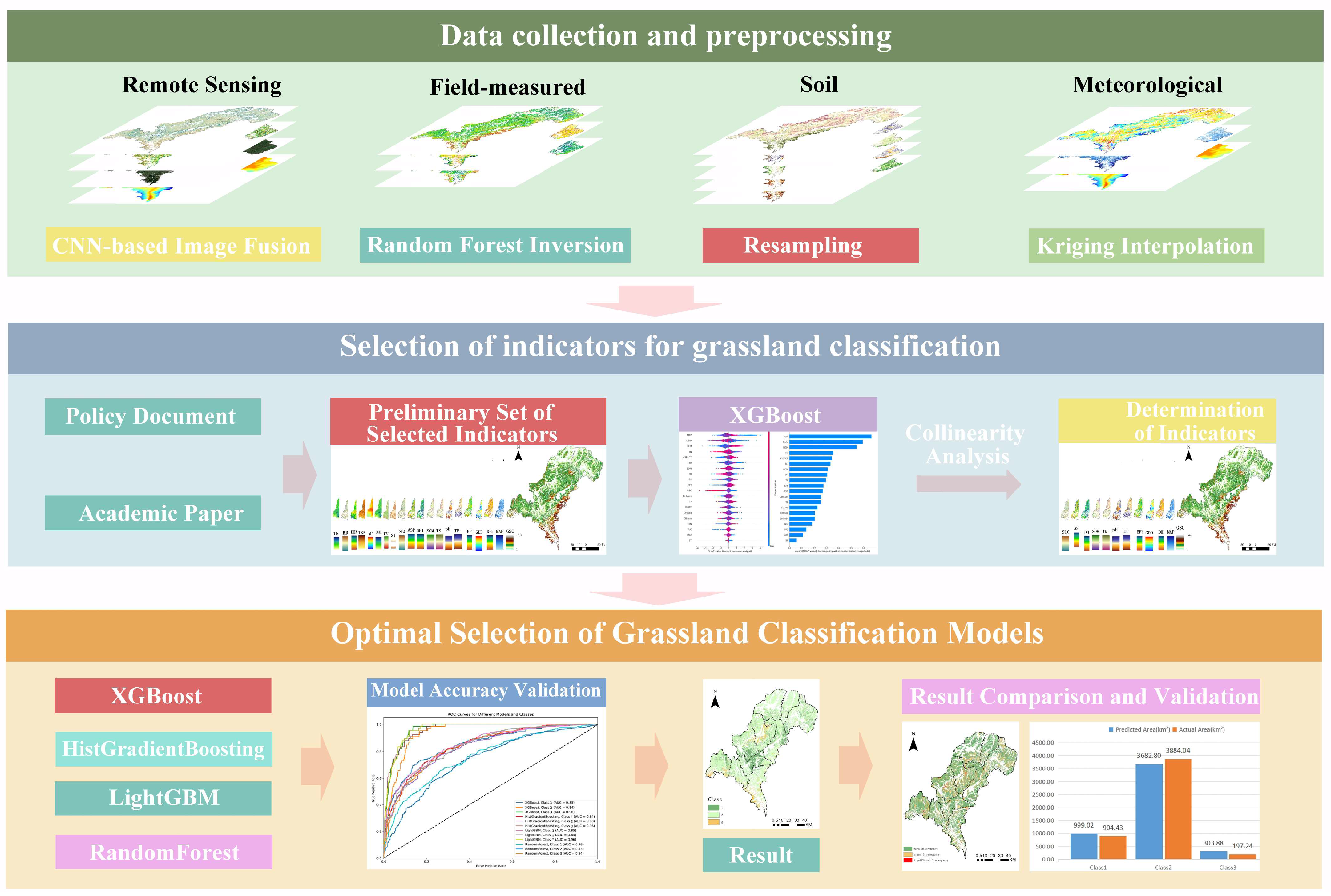
Figure 1. Research approach.
Agriculture 15 02503 g001
Figure 2. Study Area.
Agriculture 15 02503 g002
Figure 3. Comparison of remote sensing images before and after fusion (a) Original Landsat 8 image (30 m); (b) Fused image (15 m).
Agriculture 15 02503 g003
Figure 4. Feature importance of all Indicators (95% CI). (a) SHAP value (impact on model output); (b) Mean (SHAP value).
Agriculture 15 02503 g004
Figure 5. Spatial Distribution Map of the Indicators. (a) MAP; (b) AT; (c) ASPECT; (d) SOM; (e) pH; (f) TK; (g) EFY; (h) GSC; (i) DHIcum; (j) TP; (k) SLOPE; (l) DHIsea.
Agriculture 15 02503 g005aAgriculture 15 02503 g005b
Figure 6. ROC Curves for Different Models and Classes.
Agriculture 15 02503 g006
Figure 7. Model prediction results of grassland classes in Hongyuan county.
Agriculture 15 02503 g007
Figure 8. Actual grassland classes of Hongyuan County in 2022.
Agriculture 15 02503 g008
Figure 9. Area comparison between predicted and actual results.
Agriculture 15 02503 g009
Figure 10. Spatial distribution of the grassland class discrepancies.
Agriculture 15 02503 g010
Table 1. Data source and description.
Primary CategorySubcategory DataContentSensorAcquisition TimeResolutionData Source
Ground-based measured dataVegetation coverPlot coverage values July 2022Quadrat scale
(1 m × 1 m)
Self-collected by the research group
Edible forage yieldDry weight per quadrat (g/m2) July 2022Quadrat scale
(1 m × 1 m)
Self-collected by the research group
Remote sensing image dataLandsat 8Multispectral imagery(B1–7)OLIJuly 202230 mhttp://glovis.usgs.gov/ (accessed on 1 July 2024.)
Panchromatic band July 202215 m
MOD15A2FPAR dataMODIS2022500 mhttps://earthdata.nasa.gov/ (accessed on 1 July 2024.)
ALOS DEMDigital Elevation ModelPALSAR L2006–201112.5 mhttps://search.asf.alaska.edu/ (accessed on 7 Jue 2024.)
Meteorological DataAir TemperatureMean annual temperature, >0 °C accumulated temperature 2002–2022Station scalehttp://www.geodata.cn (accessed on 1 July 2024.)
PrecipitationMean annual precipitation 2002–2022Station scale
Soil DataSoil Chemical PropertiesSoil organic matter,
Soil texture,
Total nitrogen, Total phosphorus, Total potassium, pH
2009–201990 m/1 kmThe High-Resolution National Soil Information Grid of China, a dataset published by the Institute of Soil Science, Chinese Academy of Sciences (ISSAS).
Soil Physical Propertiessurface soil gravel content 2009–20191 km
Table 2. Initial set of grassland classification indices.
FactorsFull Name of IndicatorAbbreviation
ClimateMean Annual TemperatureMAT
Mean Annual PrecipitationMAP
>0 °C Accumulated TemperatureAT
TopographySlopeSLOPE
AspectASPECT
ElevationELEV
SoilSoil ThicknessTKN
Soil Organic MatterSOM
Soil TextureST
surface soil gravel contentGSC
potential of HydrogenpH
Total PotassiumTK
Total NitrogenTN
Total PhosphorusTP
Soil Bulk Density BD
VegetationVegetation CoverageFVC
Edible Forage YieldEFY
cumulative annual productivityDHIcum
annual minimum productivityDHImin
seasonal variation in productivityDHIsea
Table 3. Comparison of the Fusion Quality of CNN and GS Methods.
ModelB1B2B3B4B5B6B7Total
RMSECNN0.020.030.030.040.090.060.050.0524
GS0.080.090.10.120.410.220.180.2026
PSNRCNN27.4326.732.730.1243.4140.6335.9125.73
GS22.1621.5227.6624.737.0935.2230.419.86
Table 4. Results of the collinearity analysis among all indicators.
VariableStandardized Coefficientst-StatisticSigToleranceVIF
MAP−0.231−7.0950.0000.1666.007
AT−0.113−5.6390.0000.4382.281
TK−0.058−2.9150.0040.4432.260
EFY0.0996.4580.0000.7541.327
PH−0.076−3.4200.0010.3552.817
ASPECT0.0584.3030.0000.9791.021
SOM0.0842.5020.0120.1556.443
BD0.0010.0300.9760.1576.382
ELEV0.2627.4520.0000.1427.021
TN−0.203−5.6490.0000.1367.340
DHIcum0.0221.1560.2480.5081.967
DHIsea−0.012−0.7030.4820.5631.776
GSC−0.142−7.6740.0000.5161.938
SLOPE−0.088−5.2250.0000.6191.615
TP0.0543.3080.0010.6661.501
Table 5. Results of the collinearity analysis among retained indicators.
VariableStandardized Coefficientst-StatisticSigToleranceVIF
MAP−0.111−4.14800.2484.025
GDD−0.126−6.4900.4742.108
TK−0.011−0.6160.5380.5811.722
EFY0.0815.3100.7731.293
PH−0.148−7.14200.4182.392
ASPECT0.0634.63300.9831.018
SOM−0.037−1.8060.0710.4342.304
DHIcum0.0070.3650.7150.5161.936
DHIsea00.0090.9930.6041.655
GSC−0.147−7.92900.5221.915
TP0.0211.3020.1930.7211.387
SLOPE−0.056−3.59900.7371.357
Table 6. The model parameters.
Modellearning_ratemax_depthn_estimatorsmax_iter
XGBoost0.36100
HistGradientBoosting0.36 100
LightGBM0.36100
RandomForest 6100
Table 7. The accuracy validation results of each model.
ModelAccuracyPrecisionRecallWeighted F1-ScoreF1-Score Class1 F1-Score Class2F1-Score Class3
XGBoost0.8290.8180.8290.8200.5670.8960.512
HistGradientBoosting0.8120.7990.8120.8030.5240.8850.504
LightGBM0.8260.8140.8260.8180.5680.8940.496
RandomForest0.6440.7630.6450.6790.4650.7460.359
Disclaimer/Publisher’s Note: The statements, opinions and data contained in all publications are solely those of the individual author(s) and contributor(s) and not of MDPI and/or the editor(s). MDPI and/or the editor(s) disclaim responsibility for any injury to people or property resulting from any ideas, methods, instructions or products referred to in the content.