Abstract
Effectively managing agricultural practices is crucial for maximizing yield, reducing investment costs, preserving soil health, ensuring sustainability, and mitigating environmental impact. This study proposes an adaptation of the Grey Wolf Optimizer (GWO) metaheuristic to operate under specific constraints, with the goal of identifying optimal agricultural practices that boost maize crop yields and enhance economic profitability for each farm. To achieve this objective, we employ a probabilistic algorithm that constructs a model based on Clusterwise Linear Regression (CLR) as the primary method for predicting crop yield. This model considers several factors, including climate, soil conditions, and agricultural practices, which can vary depending on the specific location of the crop. We compare the performance of the Grey Wolf Optimizer (GWO) algorithm with other optimization techniques, including Hill Climbing (HC) and Simulated Annealing (SA). This analysis utilizes a dataset of maize crops from the Department of Córdoba in Colombia, where agricultural practices were optimized. The results indicate that the probabilistic algorithm defines a two-group CLR model as the best approach for predicting maize yield, achieving a 5% higher fit compared to other machine learning algorithms. Furthermore, the Grey Wolf Optimizer (GWO) metaheuristic achieved the best optimization performance, recommending agricultural practices that increased farm yield and profitability by 50% relative to the original practices. Overall, these findings demonstrate that the proposed algorithm can recommend optimal practices that are both technically feasible and economically viable for implementation and replication.
1. Introduction
Agriculture in Colombia is a fundamental pillar of the national economy, significantly impacting development and providing daily sustenance for millions of rural families [1]. However, despite its importance, the sector remains vulnerable, particularly in rural areas, due to challenges such as high production costs, limited market access, insufficient technical training, and the adverse effects of climate change (e.g., rainfall variability and droughts) [2]. These challenges, compounded by suboptimal crop management practices, have resulted in persistently low yields in recent years. This issue is particularly evident in maize crops which, despite ranking as the third most in-demand crop in Colombia, continue to exhibit low productivity [3]. Over the past 10 years, the average maize yield for traditional crops was only 1.93 tons per hectare (Tn/Ha) (see Figure 1) [4]. Therefore, transforming agriculture through the adoption of modern technologies and the implementation of efficient and sustainable management practices is essential for enhancing both crop productivity and overall profitability.
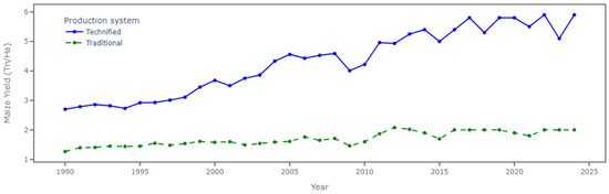
Figure 1.
Maize crop yields for technified and traditional systems from 1990 to 2024.
Traditionally, decision-making in agriculture has relied on recommendations from technicians, empirical knowledge, and practices passed down through generations. This approach often lacks a comprehensive understanding of how climate affects crops and does not consider their nutritional requirements based on the biophysical conditions of the site [5]. This limited knowledge, combined with inadequate agricultural management practices, can lead to inefficient use of essential resources such as fertilizers, pesticides, and labor. Consequently, it can result in reduced yields, significant economic losses, and negative environmental impacts [6].
To address these challenges, it is crucial to implement optimal agricultural practices that guide farmers toward more efficient use of inputs [7], adhering to principles of conservation agriculture that promote sustainability, soil health, and productivity [8]. However, factors such as difficult access to rural areas, high operating costs, and a shortage of specialized personnel significantly hinder the availability of technical assistance. As a result, many farmers lack the necessary support to improve their practices. This situation highlights the need for tools that are accessible and adapted to the local context, enabling informed decision-making that considers both the biophysical conditions of the land and the economic and logistical constraints faced by farmers.
Currently, significant advances in computing have enabled important contributions to agriculture, allowing farmers to make informed decisions on crop management [9]. Data analysis, artificial intelligence, and particularly machine learning has facilitated the development of viable recommendation systems based on historical data, as in [10], where a recommendation system was proposed based on a classifier that recommends the best crop to sow, considering various environmental parameters such as soil data, climate data, humidity, pH level, NPK fertilization, and rainfall. In this study, Random Forest (RF), Decision Tree (DT), K-Nearest Neighbor (K-NN), Gaussian Naive Bayes (GNB), and Logistic Regression (LR) algorithms were analyzed, concluding that the GNB algorithm achieves the highest accuracy (99%) for this problem, or in [11] where the authors explored the use of Convolutional Neural Networks (CNNs) to detect crop diseases in real-time and provide pesticide dosage recommendations, the research focused on images of maize crops affected by rust disease. Several deep learning architectures were evaluated, including ResNet50, VGG19, VGG16, and AlexNet. The results indicated that ResNet50 outperformed the other algorithms on all evaluation metrics, including accuracy, recall, and F1-score, achieving an impressive accuracy rate of 96%. Also, in [12] a graph-based crop recommendation algorithm was developed to identify the most suitable crop for a given season, considering several factors such as nitrogen (N), potassium (K), phosphorus (P), temperature, humidity, soil pH, and rainfall. In this study, two graph models were compared: a Graph Neural Network (GNN) and a Graph Convolutional Network (GCN). The models were evaluated using K-fold cross-validation and the F1-score metric. Finally, it is concluded that GCN better captures the relationships present in the graph. Other works such as [13,14] used statistical techniques and machine learning algorithms (conditional forests, factor analysis, and multi-layer perceptron) to identify practical recommendations that affect the yield of plantain and blackberry crops.
Machine learning algorithms have been widely applied to predict crop yields and to identify patterns and relationships among variables [15,16]. However, few studies have explored their use for optimization purposes aimed at generating practical, constraint-based recommendations to improve crop yield and profitability. In contrast, metaheuristic algorithms have been extensively applied to solve complex optimization problems in fields such as traffic routing [17], financial crisis prediction [18], construction task scheduling, and electrical microgrids [19]. In the field of agriculture, numerous studies have demonstrated the effectiveness of metaheuristic algorithms in improving various aspects of crop production and resource management. For instance, Refs. [20,21] applied metaheuristic techniques to optimize farm machinery routing and resource allocation, resulting in increased crop yields. Similarly, in [22], a root zone water quality model (RZWQM) was calibrated using coordinate descent on irrigated maize data by fitting 56 soil and 3 crop parameters. This study compares three metaheuristics Differential Evolution (DE), Basin Hopping (BH), and Particle Swarm Optimization (PSO) to optimize fertilization and irrigation practices aimed at enhancing crop yields. The results showed that the methods increase yield by 7% and farm profits by 10%. Moreover, in [23,24] a model is proposed to optimize yield and soil fertility as a function of the amount of nitrogen, phosphorus, and potassium (NPK) applied to each crop. For this study, three crops were analyzed: maize, cotton, and wheat. A genetic algorithm (GA) was used to define the optimal practices for each crop, and the results showed that the model can recommend optimization patterns and increase yield.
On the other hand, the Grey Wolf Optimizer (GWO) has been widely used in agriculture due to its ability to solve complex optimization problems, enabling a balance between exploration and exploitation [24]. This algorithm is based on the way wolves hunt in packs. It replicates wolves’ leadership hierarchy and cooperative hunting to optimize solutions by modifying locations and exploring a multidimensional search space. Several studies have implemented this method due to its simplicity, speed, and its ability to address models with multiple constraints and objectives [25]. As in [26], where GWO optimizes the plantation structure in irrigated areas of China, balancing water consumption, profitability, and crop yield or in [27] where the efficient allocation of water resources in irrigation canal systems in northwest China is optimized achieving an resources efficient distribution. Also, in [28], an improved variant of the algorithm called SLEGWO was proposed, aiming to achieve accurate fertilization by optimizing the ratio of nitrogen, phosphorus, and potassium to maximize crop yield.
Previous studies have significantly contributed to the development of recommendation systems that utilize machine learning algorithms and metaheuristics. However, they often fail to consider the real constraints that farmers face, such as budget limitations, selling prices, and maximum application rates of nutrients and pesticides at various crop stages (Planting, emergence, and flowering). This limitation reduces the applicability and accuracy of recommendations for actual crop planting conditions. Therefore, in this study, we propose to adapt the Hill Climbing (HC), Simulated Annealing (SA), and Grey Wolf Optimizer (GWO) metaheuristics to address a single-objective mixed constrained optimization problem. Our goal was to generate personalized recommendations for maize crop management practices using a data-driven approach. The fitness function will be directly related to an empirical model that predicts crop yield, allowing us to maximize profitability (Profit) for the crop. These recommendations will be tailored to practical constraints to ensure their viability, considering essential factors such as the farmer’s budget, selling prices of the product, and specific limitations that may affect crop yield.
The main contributions of this paper are: (1) The adaptation and comparison of three metaheuristic algorithms focused on optimizing agricultural management practices to maximize maize crop profitability, considering the constraints faced by farmers. (2) The comparison of several machine learning techniques to predict maize crop yield according to a substantial number of variables related to soil, climate, and agricultural management practices, among others. (3) The adaptation of a new Clusterwise Linear Regression (CLR) approach to predict maize crop yield, which achieves the best results compared to traditional techniques.
Unlike previous research, this work integrates a probabilistic CLR model with an adapted Grey Wolf Optimizer, explicitly incorporating economic and agronomic constraints. This approach enhances the realism and applicability of the recommendations generated.
The rest of this paper is organized as follows: Section 2 describes the dataset used for the study, the machine learning algorithms implemented to predict crop yield, the fitness function that the metaheuristic algorithms seek to maximize, as well as the representation of vector solution in these algorithms and the adaptation of the metaheuristics to the specific problem. Section 3 analyzes the performance of machine learning (ML) models for predicting maize crop yield and compares the results obtained using metaheuristic algorithms based on HC, SA, and GWO to optimize the agricultural management practices. Finally, Section 4 presents the conclusions and future work that the research group expects to develop in this area.
2. Materials and Methods
For the development of this research, the CRISP-DM process served as a methodological guide to understand the problem domain, explore and prepare the data, build and evaluate models, and select the machine learning model that best predicts maize crop yield [29]. Subsequently, to adapt metaheuristics (HC, SA, and GWO) for optimizing agricultural practices, the iterative research pattern proposed by Pratt was employed [30]. Each artifact used in the study is described below.
2.1. Dataset
This study utilized a dataset collected from maize crops in the Department of Córdoba, Colombia, between 2014 and 2018. FENALCE, in collaboration with CIAT, collected various variables influencing maize crop yield, including climate variables, soil variables, and agricultural management practices [31]. For this study, the dataset presented in [32] was used, in which various data mining techniques were previously applied to preprocess the variables and generate new attributes, thereby improving dataset quality and enhancing predictive performance. The original dataset comprises 799 observations and 114 variables, with each observation representing a single crop event recorded by farmers over a four-year period.
2.2. Machine Learning Algorithms
Before beginning the optimization process, it was necessary to select a suitable machine learning algorithm for predicting maize crop yield. Previous studies have employed various algorithms and techniques depending on the dataset’s structure (structured or unstructured) and the specific variable being predicted [33,34,35]. In this study, the following algorithms were evaluated: Elastic Net Linear Regression (LR), Random Forest (RF), Bagging Regressor (Bootstrap Aggregating), Multi-Layer Perceptron (MLP), and a new method based on Clusterwise Linear Regression (CLR) [36].
The CLR-based approach is a probabilistic method that utilizes the Gaussian Mixture Model (GMM) to create an undetermined number of clusters [37]; subsequently, it creates linear regression models for each cluster using Elastic Net regression to predict the crop yield and applies the Decision Tree (DT) algorithm to classify a new observation (crop) into one of the previously created groups or clusters. Figure 2 shows the flow chart of the designed probabilistic algorithm that builds the CLR model in the following stages:
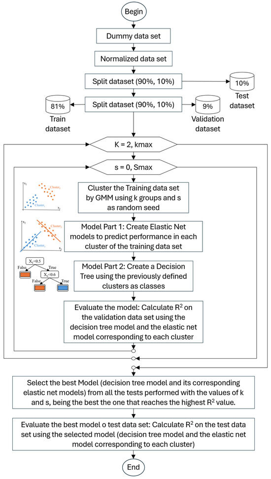
Figure 2.
Flowchart of the algorithm creating the Clusterwise Linear Regression model.
- Preprocessing: This process involves several tasks. First, we dummy-code the variables that require it to create a mineable view, which is a matrix composed solely of numerical data. Next, we perform a normalization process using Min-Max normalization to ensure that differences in the variable ranges do not impact the subsequent clustering analysis. After normalization, we create three datasets: a Training dataset, which contains 81% of the total instances from the input dataset; a Validation dataset, which includes 9% of the instances; and a Test dataset, which accounts for the remaining 10%. These datasets were created as random samples without replacement, ensuring that the original dataset is fully partitioned into the three sets.
- CLR models construction: To perform this process, different numbers of groups and seeds per group must be evaluated, since the clustering process is probabilistic and produces varying result quality depending on the random seed defined for the execution of the algorithms and that the number of groups is not known a priori to the execution of the clustering algorithm. In this case, a specific number of groups (k) is evaluated from two (2) to a maximum number of groups (kmax), which can be defined as a function of the number of observations (n) in the dataset as √(n⁄2), or a specified number established by the user. For the number of seeds, a maximum (Smax) is set, which can be defined a priori, and in the tests was set to 31. Based on these two values (number of groups -k- and random seeds -rs-), two nested cycles are performed that include four essential steps, namely:
- Clustering: With the training dataset, the data are clustered (using only the predictor or independent variables -X- and not the target or dependent variable -y-) using the Gaussian Mixture Models (GMMs) algorithm, considering the k and s values. In the design process of probabilistic algorithms, both K-Means clustering and Spectral Clustering algorithms were evaluated; however, the Gaussian Mixture Model (GMM) demonstrated superior performance, and it was selected.
- Regression (Part 1 of the model): A linear regression model was developed for each group using Elastic Net. Given the high dimensionality of the dataset, Elastic Net was employed to apply both Lasso (L1) and Ridge (L2) penalties. This approach helps eliminate potential collinearity among the independent variables and selects the most relevant features for each group. As a result, the model is less likely to overfit the data and demonstrates better generalization.
- Classification (Part 2 of the model): This stage receives as input a training dataset that includes the predictor or independent variables (X), and the dependent variable (y), which refers to the groups or clusters assigned to each observation from the previous clustering step. After evaluating several classifiers, we selected the Decision Tree due to its excellent performance and ease of interpretation. The output of this step is a classification model, specifically a decision tree, which enables new observations to be classified into one of the predefined groups or clusters.
- Model evaluation: The quality evaluation process is conducted based on the developed model, which includes a decision tree and regression models for each group or cluster. To perform this evaluation, a validation dataset is used, which contains the variables X and their corresponding variable y, representing the crop yield. Each record in this dataset first defines the group or cluster to which it belongs using the decision tree algorithm. Then, the regression model for that group is applied, and the yield is predicted, yielding the y_predicted value. With all the values of y and y_predicted, the coefficient of determination (R2) is calculated. The development model and its R2 value are stored in a list to select the best one.
- Selection of the best CLR model: From the list of generated models with their R2, the one with the best R2 value (highest) is selected. This selected model is then used in the validation or prediction phase when it is moved to a production environment.
- CLR model validation: Based on the model selected as the best (formed by the decision tree and the regression models of each group or cluster), the quality evaluation process is conducted. This stage is similar to “Model evaluation” stage; the only change is the dataset used, which in this case is the validation dataset and not the test dataset. High and similar R2 values in the test and validation datasets confirm an appropriate fit of the obtained model. Other metrics used in the algorithm selection were the mean squared error (MSE) and mean absolute error (MAE). It should be noted that when the model is used for prediction, the input data must first undergo the same preprocessing (dummification and MinMax normalization using the same variable ranges defined during the preprocessing stage).
The CLR model obtained outperformed other state-of-the-art regression algorithms. For this reason, it was selected to predict maize crop yield and to define part of the objective function (fitness function) used for optimizing the agricultural management practices presented below.
2.3. Adaptation of Metaheuristics
For the optimization process, three algorithms widely recognized in the literature due to their simplicity and efficiency in solving complex optimization problems were adapted. First, we adapted the Hill Climbing (HC) algorithm, a single-state heuristic, not a metaheuristic, known for its simplicity and efficiency in optimizing unimodal problems [38]; HC was only included to compare results against metaheuristics. Second, we adapted the Simulated Annealing (SA) algorithm, based on the principle of metal cooling, which maintains a balance between exploration and exploitation by varying a parameter known as temperature, which decreases with time or the number of evaluations of the objective function (EFOs) used in the search and optimization process; this single-state metaheuristic algorithm uses directional changes in the search to avoid being trapped in local optima and optimize separable and non-separable multimodal problems with excellent results [39]. Finally, the Grey Wolf Optimizer (GWO), a population metaheuristic inspired by the hunting behavior of grey wolves, was adapted [24]. This algorithm models the hierarchical pack structure, where alpha, beta, and delta wolves lead the process of searching and optimizing solutions to solve a wide range of optimization problems efficiently. Key parameters for each algorithm, including cooling schedules for SA and population size for GWO, are detailed in Section 2.3.6.
For the optimization process, variables related to crop management were selected from the dataset as the variables to be optimized. Soil variables such as: Observe Moho Rasta (Observe_Moho_Rasta), Soil Percentage with Clayey texture (Porc_A), Soil Percentage with silty texture (Porc_L), among others and climate variables as: Average maximum temperature in vegetative stage (Temp_Max_Avg_Veg), Accumulated precipitation in formation stage (Rain_Accu_For), Accumulated solar energy in maturity stage (Sol_Ener_Accu_Mad), among others are not optimized because they are no in the farmer’s control. Table 1 displays each variable to be optimized, its meaning, and the corresponding range of values.

Table 1.
Details of variables to be optimized related to maize crop management.
The following describes the fitness function and the adaptation of the metaheuristics considering the constraints specific to the problem.
2.3.1. Fitness Function
To evaluate the performance of the metaheuristics and HC, the fitness function is defined as shown in Equation (1), where the objective is to maximize the crop profit, i.e., maximize (G).
where
- G refers to the net profit in pesos associated with a crop event.
- P is the maize crop yield expressed in Kg-Ha. This value is predicted using one of the machine learning algorithms, specifically the CLR algorithm, which obtained the most accurate results.
- SP refers to the selling price of one Kg of white maize, expressed in COP$/Kg.
- CP refers to the production costs associated with each event (crop); a value that corresponds to the sum of the costs associated with the values used in each of the variables to be optimized. That is:. Where are the values of the variables of each of the 22 variables (m = 22) being optimized and is the market cost of the unit of each variable per hectare (COP$/Ha).
- B corresponds to the farmer’s maximum budget allocated for cultivating the crop.
The constraints of this problem are:
- The possible value for each continuous variable (Float) is assigned between the minimum and maximum values allowed for each of the variables. That is: . If a variable exceeds the permitted range, its value is set to the limit value it overflowed.
- For the case of integer variables (binary, ordinal, or nominal), the value is set as an integer value in the range of possible values, including limits. That is: . In the logic of optimization algorithms, it is ensured that a valid value is always assigned.
- Solutions that exceed the farmer’s maximum budget (B) will be discarded, and new solutions will be sought. In other words, the optimization process does not attempt to repair solutions that violate the budget constraint.
- In the optimization process for the three algorithms, the soil and climate variables remain unchanged; only the variables related to agricultural practices are modified.
2.3.2. Solution Vector Representation
Figure 3 illustrates the solution vector, which comprises a combination of categorical and continuous variables. This vector includes all the variables related to soil, climate, and crop management practices. However, only the crop management variables are optimized. As previously mentioned, climate and soil variables remain fixed because they are factors that farmers cannot control or manipulate.
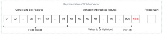
Figure 3.
Solution vector representation for the optimization process of agricultural practices.
The yield variable is an integral part of the solution vector and represents the prediction generated by the machine learning model, specifically the CLR model. This prediction is based on the values of all the independent variables, including soil, climate, and crop management practices, which are included in the solution vector. It is important to note that this solution vector is transformed and formatted to meet the requirements of the machine learning model used to estimate crop yield. This process enables the calculation of estimated yield, which can subsequently be used to evaluate the fitness function (Profit).
After calculating the crop yield, the cost of the crop is determined by assessing the expenses associated with each variable that needs optimization. These costs can be adjusted based on the financial circumstances and demand conditions faced by each farmer. Finally, using the previously recorded maize selling price, the fitness (Profit) linked to the solution is calculated according to Equation (1).
Given that the Grey Wolf Optimizer (GWO) achieved the best results in the experiments, we will first explain this method, followed by Hill Climbing, and then Simulated Annealing.
2.3.3. Grey Wolf Optimizer (GWO) for Mixed Constrained Optimization
The Grey Wolf metaheuristic algorithm is inspired by the social behavior of grey wolf packs and their organization for hunting activity [40,41]. Within the algorithm, three fundamental stages are identified.
Definition of the hierarchy: The fundamental pillar of the search process begins by identifying the three best solutions in the population, which represent the alpha, beta, and delta wolves. The alpha wolf is responsible for making decisions about hunting and leading the pack. The second level of the hierarchy consists of beta wolves, who assist in decision-making and follow the alpha’s orders; finally, the third level is composed of delta wolves who are scouts, hunters, and caretakers. In [40] a mathematical model is exposed to represent the hierarchy of wolves, where one has a population of wolves represented by the set , where each vector, being an individual of the population and the number of dimensions of the optimization problem. In the algorithm, the three best solutions of the population, alpha , beta and delta , are selected according to the objective function to be optimized.
Tracking and hunting prey: This refers to the behavior of wolves encircling the prey, where each wolf in the population adjusts its position based on the reference points set by the alpha, beta, and delta wolves, intending to find an optimal position. This movement is shown in Equation (2).
Completion and evaluation: The search and hunt conclude when a convergence criterion is met. The alpha wolf () represents the best solution to the optimization problem.
Algorithm 1 presents the adaptation of the Grey Wolf Optimizer (GWO) for optimizing maize crop management practices. In line 2, the wolf population is randomly initialized. Each variable is assigned values uniformly within the designated range for continuous variables or uniformly among the available values for discrete or binary variables. In line 3, the fitness function is calculated using the values from the solution vector, along with the predetermined costs, the maize selling price, and a machine learning model that predicts maize yield. Line 4 ranks the wolf population based on fitness, placing the most fit individuals at the beginning.
Subsequently, between lines 6 and 17, an iterative process is conducted to search for the best solution to this problem. Lines 6 to 8 define the agents (alpha, beta, and delta wolves) that guide the search during each iteration, along with their respective fitness levels. Lines 9 to 11 define the control parameters (a, A1, A2, A3, C1, C2 and C3) that govern the exploration and exploitation processes of the algorithm, which allow discovering promising areas to converge towards a global optimum; Rnd (0,1) refers to a random real number uniformly generated between 0 and 1. In lines 13 to 15, each agent in the population is traversed to search for a potentially better position, denoted as r (line 13). The quality of this new position, r, is then evaluated (line 14), and if it has superior quality, the current agent is replaced by the position r and its quality. The process of updating each wolf’s position is further elaborated in Algorithm 2. By line 17, the population of wolves is sorted by fitness at each iteration, allowing the agents guiding the search (alpha, beta, and delta wolves) to be redefined. The algorithm finally returns the alpha wolf as the optimal solution, along with its corresponding fitness value.
| Algorithm 1. GWO adaptation to optimize the maize crop management practices | |
| Inputs: | s: Record to be optimized previously dummified and normalized. lvo: List of variables to be optimized with their associated type (continuous or categorical), their possible values, and their associated costs. b: Farmer’s maximum budget. pv: Maize selling price. mlm: Machine learning model that calculates the maize crop yield. plocal: Exploitation probability for categorical variables. popsize: Size of the wolf population. max_iter: Maximum number of iterations, where max_efos = max_iter × popsize. |
| Output: | : Best solution in the population : Quality of best solution |
| |
The main difference in the present algorithm from the traditional GWO algorithm proposed in [42] is presented in line 13, where the position of the agent (wolf) is updated according to the type of variable (continuous or categorical); Algorithm 2 details this process.
In line 2 of Algorithm 2 a copy of the wolf that is to be updated is created. Then, in lines 3 and 4, two separate lists are generated: one for continuous variables and another for categorical variables. Next, in lines 5 to 9, the continuous variables of the wolf are updated using the classic formula of the Grey Wolf Optimizer (GWO) algorithm. In this formula, each new value of a variable is calculated as an average of the three main wolves (alpha, beta, and delta). However, modifications are made to include the current wolf’s value for the same variable, along with the respective A and C values for each wolf, as detailed in lines 6, 7, and 8. It is essential to ensure that any assigned continuous values remain within the defined limits of each variable. If a value exceeds these limits (either the upper or lower threshold), the limit value is assigned in its place.
The handling of the categorical variables is different; this is conducted in lines 10 and 11 where the variables are run through one by one and assigned in r according to a random selection of the values that have the alpha, beta, delta, and current wolves; this selection occurs with a probability denoted as p_local, which is a float value between 0 and 1. When p_local is higher (closer to 1), there is a greater tendency to perform a local search around the values of the alpha, beta, delta, and current wolves, resulting in less exploration of other possible values for the variable. Conversely, if p_local is lower, a random selection is made from all possible values of the variable. Finally, the new solution, denoted as r, is returned to the current wolf, w.
| Algorithm 2. Wolf movement adaptation in GWO for mixed variables | |
| Inputs: | w: Current wolf. : Alpha wolf. : Beta wolf. : Delta wolf. A1, A2, A3: Alpha, beta, and delta wolf exploitation factors. C1, C2, C3: Alpha, beta, and delta wolf exploration factors. plocal: Local exploitation probability for categorical variables. lvo: List of variables to be optimized with their associated type (continuous or categorical), their possible values, and their associated costs. |
| Output: | r: Possible new position of the current wolf w. |
| |
2.3.4. Hill Climbing (HC) for Mixed Constrained Optimization
The adaptation of the Hill Climbing algorithm for this problem is outlined in Algorithm 3. In line 2, a random initialization of a candidate solution (S) is performed based on the input record (s) and the list of variables to be optimized, which includes the ranges and costs associated with each variable. The values of the variables to be optimized are randomly initialized within their respective ranges. Then, in line 3, a machine learning model is called to calculate the yield, which is stored in the yield field of the solution S. Additionally, the production cost is computed, and considering the selling price and the farmer’s budget, the fitness of the solution is calculated and recorded.
Between lines 4 and 9, an iterative process is performed to improve the solutions. In line 5, a solution R is created and generated by applying minor modifications to the current solution S. The changes are described below and refer to the mixed_tweak operator. Subsequently, in line 6 the fitness evaluation of the new solution R is performed and in line 7 the quality of solutions R and S is compared; if the quality of R is better than that of S, solution S is replaced by solution R (line 8) and this new solution S is the one that is optimized in the next cycle. The algorithm runs a maximum number of EFOS and returns the best solution S found in the search process. The main difference between this algorithm and the original HC algorithm [39] lies in how to manage the list of variables (both categorical and continuous) that need to be modified within their respective data ranges, as well as the adjustment of the mixed_tweak operator.
The mixed_tweak operator begins by selecting a specific number of variables, V, to be modified. By default, V is set to 3, which represents 12% of the total variables involved in optimizing crop management practices. For each selected variable, a slight modification or adjustment is applied depending on the variable’s type. If the variable is continuous, a randomly generated value is added, ranging from -bandwidth to +bandwidth, defined for that variable. The new value is then checked to ensure it falls within the valid limits. If it exceeds these limits, it is adjusted to the nearest valid limit. For binary variables, the current value is inverted (0 ↔ 1). For non-binary discrete variables, one of the possible values is randomly assigned, ensuring that it is different from the current value.
| Algorithm 3. Adaptation of the HC algorithm to the optimization problem of maize crop management practices | |
| Inputs: | s: Record to be optimized previously dummified and normalized. lvo: List of variables to be optimized with their associated type (continuous or categorical), their possible values, and their associated costs. bw: Bandwidth vector for each variable. pv: Maize selling price. b: Farmer’s maximum budget. mlm: Machine learning model that calculates crop yield. max_efos: Maximum number of evaluations of the objective function. |
| Output: | S: Best solution found. : Quality of the best solution found. |
| |
2.3.5. Simulated Annealing (SA) for Mixed Constrained Optimization
The adaptation of the Simulated Annealing (SA) algorithm is presented in Algorithm 4. This algorithm is like HC, except for the use of the temperature variable (t), which is initialized in line 4. This variable is used in line 9 to allow the possibility that a solution R with lower quality than the current solution S can be accepted, potentially changing the direction of the optimization toward another point in the search space. Finally, in line 11, the temperature value is decreased, ensuring that as iterations progress, poor solutions have a lower probability of being accepted to replace the current solution S. Additionally, a new variable, called best, along with its corresponding quality or fitness, is introduced. This variable is initialized in line 5 with the first randomly generated solution and then updated in the iterative process in line 13 when a found solution is better than the current best. This variable and its quality are the ones returned by the algorithm because they represent the best solution found in the search process.
| Algorithm 4. Adaptation of the Simulated Annealing algorithm to the optimization problem of maize crop management practices | |
| Input: | s: Record to be optimized previously dummified and normalized. lvo: List of variables to be optimized with their associated type (continuous or categorical), their possible values and their associated costs. bw: Bandwidth vector for each variable. pv Maize selling price. b: Farmer’s maximum budget. mlm: Machine learning model that calculates crop yield. max_efos: Maximum number of evaluations of the objective function. |
| Output: | S: Best solution found. : Quality of the best solution found. |
| |
2.3.6. Configuration Parameters for ML Algorithms and Metaheuristics
In the first part of the research, the objective was to develop a machine learning algorithm to predict maize crop yield. Table 2 lists the algorithm’s parameters used in this process. These values were the ones that, after a process of refinement, obtained the best results.
Table 2.
Hyperparameters for each machine learning algorithm.
In the second part of the research, which focused on optimizing agricultural management practices through the most effective machine learning model and fitness function, we used the best parameters of each metaheuristic algorithm (Hill Climbing, Simulated Annealing, and Grey Wolf Optimization) as presented in Table 3. The search for and selection of the best parameters were conducted using 80 randomly selected records from the original dataset.
Table 3.
Hyperparameters for each metaheuristic.
3. Results and Discussion
This section presents the performance results of the machine learning models, along with the respective density curves for the HC, SA, and GWO metaheuristics, identifying the most effective algorithm for optimizing maize crop management practices. Additionally, it includes examples of optimized crops, highlighting practices that have led to improved yields and increased profits.
3.1. Performance of Maize Crop Yield Prediction Models
To evaluate the performance of the machine learning models, the dataset was split into a training set (90%) and a test set (10%). Figure 4, Figure 5 and Figure 6 illustrate model performance using the coefficient of determination (R2), Mean Absolute Error (MAE), and Root Mean Squared Error (MSE) as evaluation metrics.
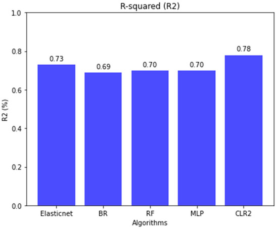
Figure 4.
Performance comparison of ML models using the metric determination coefficient.
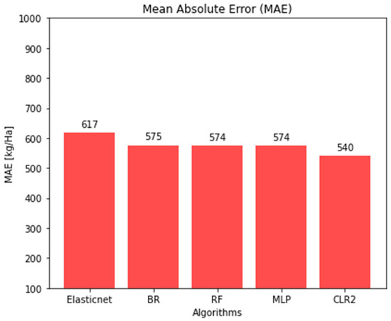
Figure 5.
Performance comparison of ML models using the metric MAE.
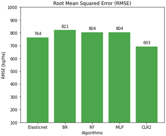
Figure 6.
Performance comparison of ML models using the metric RMSE.
Figure 4 displays the R-squared (R2) values obtained from various machine learning algorithms used to predict maize crop yield. The x-axis shows the algorithms evaluated: Elastic Net (Elasticnet), Bagging Regressor (BR), Random Forest (RF), Multi-Layer Perceptron (MLP), and Clusterwise Linear Regression with two groups (CLR2). The y-axis represents the R2 values, expressed as percentages, which indicate the proportion of variance in the dependent variable explained by each model. Higher R2 values signify better predictive performance. CLR2 achieves an R2 value of 78% for the test data, outperforming the Elastic Net model, which achieves 73%. The other algorithms (BG, RF, and MLP) all reach R2 values of around 70%.
Figure 5 shows the Mean Absolute Error (MAE) for the same set of algorithms. The x-axis lists the models, while the y-axis represents MAE in kilograms per hectare (Kg-Ha), measuring the average magnitude of prediction errors regardless of direction. Lower values indicate greater accuracy. Among the models, CLR2 achieved the lowest MAE (540 Kg-Ha), indicating superior performance. In contrast, Elastic Net showed the highest MAE (617 Kg-Ha), reflecting the poorest performance. The BR, RF, and MLP algorithms produced similar MAE values, all around 575 Kg-Ha.
Finally, Figure 6 shows the Root Mean Squared Error (RMSE) values, which represent the average squared difference between predicted and actual (true values), with larger errors being penalized more heavily. As in the previous figures, the x-axis identifies the models, and the y-axis indicates RMSE in Kg/Ha. CLR2 achieved the lowest RMSE (693 Kg-Ha), confirming its high performance. In contrast, BR recorded the highest RMSE (821 Kg-Ha), while RF and MLP both showed intermediate results (804 Kg-Ha).
When comparing the performance of the CLR2 model against more complex models, such as the Bagging Regressor (BR), Random Forest (RF), and Multi-Layer Perceptron (MLP) models, it was observed that the results obtained by the CLR2 model are close to those obtained by the more complex models. However, due to their complexity, these models are considered “black boxes,” offering little to no interpretability or transparency. Therefore, additional tools, such as SHAP and LIME, are required to interpret model predictions. Conversely, the CLR2 model is easily interpretable because it is primarily composed of a decision tree and two regression models, which are among the most interpretable models in artificial intelligence. The linear model obtained with Elastic Net is simpler and easier to interpret; however, it has an R2 value 5% lower than the CLR2 model.
3.2. Metaheuristics Performance Evaluation
To evaluate the performance of HC, SA, and GWO metaheuristics, 50% of the records of the original dataset, i.e., 398 crop events, were optimized. These 398 records were randomly selected from the original dataset. To assess the quality of results, each algorithm was run 30 times per crop using different random seeds. Ultimately, the average profit (fitness) for each algorithm (HC, SA, and GWO) was determined for each crop. Figure 7 displays the density plots for the three metaheuristics, generated from the optimization of the 398 crop events. It can be clearly observed that the GWO algorithm achieves the highest average profit (μ = 21.07 million) compared to the other algorithms. HC obtained the second-best average profit (μ = 15.40 million), while SA recorded the lowest performance, reaching an average profit (μ = 14.46 million). This figure also reports that the minimum values reported by HC and SA are below 6 M, while the one reported by GWO is above 10 million. Likewise, the highest values reported by HC and SA are just around 22.5 million, while GWO reaches 30 million. Notably, HC tends to follow a normal distribution, though it shows slight peaks or ‘mountains’ that introduce right-skewness, where better results are typically observed. It is also observed that SA has an asymmetric distribution to the right, like that of HC. Although SA has the potential to find better solutions than HC by having a mechanism to escape from local optima, it is observed that it requires more evaluations of the objective function to utilize this capability. GWO, on the other hand, shows better performance than SA and HC, with higher average profit, but they have higher variance with respect to the other algorithms; GWO exhibits greater symmetry; however, it displays a distinct behavior by generating two ridges around the mean. Further investigation is needed to analyze this phenomenon in future work.

Figure 7.
Density curve comparison between HC, SA, and GWO algorithms for 400 crop events.
Finally, to identify whether there is a statistically significant difference between the results obtained for each of the metaheuristics, the Friedman nonparametric statistical test was applied [43]. Table 4 summarizes the results obtained, showing that GWO achieves the best performance (Ranking 1), followed by HC (Ranking 2) and SA (Ranking 3). Considering that the p-value obtained with the Friedman test was it can be concluded that at least one of the algorithms performs differently from the others. Due to the above, we proceeded to perform the Wilcoxon statistical test as a post hoc analysis of the Friedman test. Table 5 shows the results obtained with the Wilcoxon test. The symbol ● means that the method in the row reports better results than the method in the column and the symbol ○ means that the method in the column reports better results than the method in the row. In addition, the results above the diagonal indicate a 90% statistical confidence, while the results below the diagonal indicate a 95% confidence level. It can be concluded that GWO reports better results than SA and HC with 95% confidence, and HC reports better results than SA with 95% confidence. Iman and Davenport, as well as Nemenyi’s post hoc analysis, reported the same conclusions.
Table 4.
Ranking obtained with the Friedman test.
Table 5.
Summary of the Wilcoxon test results.
3.3. Effect of Optimizing Maize Crop Management Practices
To evaluate the impact of optimizing crop management practices using the GWO algorithm, we compared the results obtained from the GWO algorithm with the original, unoptimized records. To determine the yield of the original crops, we ran the CLR model for each crop. We then calculated the profit for each event (baseline) based on the costs and selling price of maize. Figure 8 presents the results from the GWO optimization alongside the baseline data. The use of the optimizer resulted in an average profit increase in COP$9.7 million compared to the baseline. This increase is attributed to the direct relationship between profit and yield; improvements in crop management practices led to significantly higher yields at lower costs, enhancing profitability.
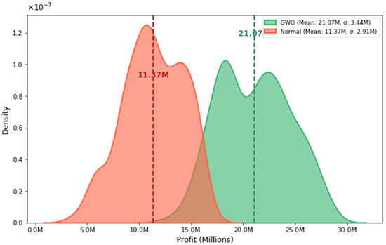
Figure 8.
Comparison between the current profit (Normal) obtained without performing optimization of agricultural variables vs. the profit after performing crop optimization using GWO.
Finally, Table 6 presents three examples of optimized individual cropping scenarios. It compares current management practices with optimized practices, as well as the yield and profit obtained in both scenarios. In these examples, yield improvements range from 42 to 118% and profit from 36 to 96%.
Table 6.
Details of the management practices being optimized and the expected results in yield and profit for four cropping events. * Indicates optimized practices.
3.4. Deployment in a Web Application
As part of this research, a web application was developed using the Django framework in Python version 3.11, which integrates the core modules for crop prediction and recommendation. The objective of this application is to provide farmers with accessible and user-friendly tools that support data-driven decision-making in agricultural management. The two most relevant functionalities of the application are described below.
Figure 9 shows the graphical interface of the prediction module, which internally applies the CLR2 algorithm to estimate maize yield for each registered crop. In its current version, the application requires the registration of 114 input variables per crop, related to climate, soil characteristics, and agricultural management practices. In future versions, the number of climate-related variables will be reduced, as these can be automatically retrieved from the georeferenced location of the crop using climate AI services.
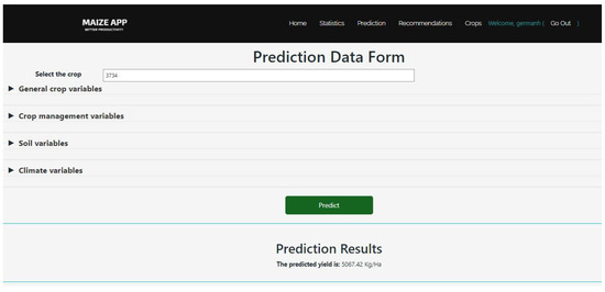
Figure 9.
Graphical user interface for maize yield prediction module in the Maize App web application.
Figure 10 presents the graphical interface of the recommendation system, which incorporates the GWO algorithm. This algorithm takes as input the crop data, the maize market price, the farmer’s budget, and the unit costs of each management variable. Based on these inputs, it generates estimates of expected yield, profit, and implementation costs for the recommended agricultural practices.
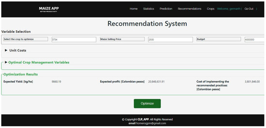
Figure 10.
Graphical user interface for recommendation system module in the Maize App web application.
The results are provided as clear and actionable recommendations, complemented by interactive dashboards. These dashboards present key performance indicators (KPIs) through descriptive analytics, thereby enhancing the system’s usability and reinforcing its capacity to support data-driven decision-making in agricultural management.
The proposed models were developed in Python and executed efficiently on HP personal computers (HP Inc., Palo Alto, CA, USA) with an Intel Core i5 processor, CPU with 4 cores, 16 GB RAM, and a 128 GB SSD. Notably, the CLR2 model can be stored and executed locally on smartphones with suitable response times. The GWO can also be adapted for local execution on smartphones; however, its runtime depends largely on the device’s processing capacity and the number of objective function evaluations configured for its execution.
3.5. Limitations
- In CLR, the execution time or complexity of the training process is determined by the number of random number seeds (s) and the number of groups to be evaluated (k). A larger number of seeds and groups will take longer time for the algorithm to find the optimal data distribution.
- The CLR approach proposed is based on linear regression models which are sensitive to outliers, so it is crucial to handle them properly during the data preprocessing stage to ensure the CLR model’s performance is not compromised.
- CLR, like any machine learning model, requires a thorough data cleaning and transformation process, aimed at creating a solid mineable view that can effectively inform algorithms.
- The dataset employed to train the machine learning models was collected in the Department of Cordoba, Colombia, and comprises 114 variables related to climate, soil, characteristics and agricultural management practices. The resulting model is specific to this region and cannot be directly generalized to other areas due to the spatial and temporal variability to which maize crops are exposed. Consequently, the findings may not be transferable to regions with different climatic or socioeconomic conditions, underscoring the need for validation using locally collected datasets.
- The current implementation of Hill Climbing, Simulated Annealing, and Grey Wolf Optimizer algorithms involves exploring only the feasible solution space. This means that any solution generated which does not comply with constraints is automatically discarded.
4. Conclusions and Future Work
4.1. Conclusions
The probabilistic Clusterwise Linear Regression algorithm with two groups (CLR2) provided more accurate maize crop yield predictions compared to several machine learning models, including Elastic Net linear regression, Bagging Regressor (BR), Random Forest (RF), and Multi-layer Perceptron (MLP). With CLR2, we obtained an R2 value 5% higher than the other compared algorithms, which guarantees a better fit to the data. All models used environmental, soil, and agricultural management features as predictor variables. This approach helps identify the most influential and relevant factors affecting agricultural decision-making.
The optimization algorithms successfully achieved their objective of recommending effective crop management practices by maintaining appropriate levels for each variable, thereby helping to prevent soil and environmental contamination. This approach not only reduced costs but also increased production and farm profitability.
This study presents an adaptation of the GWO algorithm for optimizing agricultural management practices under constraints, achieving satisfactory results that are both feasible and accessible to farmers, thereby facilitating real-world application. The proposed framework demonstrates potential for broader adoption; however, validation in other regions is required.
By applying the GWO algorithm to optimize agricultural management practices, a 50% improvement in crop yield and profitability was achieved compared to the baseline, demonstrating the effectiveness and theoretical relevance of the proposed approaches.
4.2. Future Works
Future work will focus on implementing additional population-based metaheuristics, such as genetic algorithms (GAs), particle swarm optimization (PSO), ant colony optimization (ACO) and Cuckoo Search (CS), to evaluate the performance of these techniques in addressing this specific problem and to compare their efficiency and accuracy with the currently implemented methods.
Currently, the adaptation of the HC, SA, and GWO algorithms is achieved by constantly evolving in the feasible solutions space. Therefore, when a solution that does not meet the constraints is created (randomly or by operators such as tweak), the solution is discarded. In this sense, and to avoid spending evaluations of the objective function, future work is expected to investigate two proposals: first, the implementation of a solution repair scheme, and second, allowing the algorithm to evolve in both feasible and infeasible space.
As future work, the recommendations for agricultural practices will be validated through field trials under real growing conditions, thereby reinforcing the applicability and reliability of the results obtained.
The development of a mobile application is planned to replace the existing web application, offering farmers a more intuitive, user-friendly, and accessible tool. In addition, the integration of geolocation (GPS) modules and climate AI services will enable the automatic retrieval of climate variables for each crop by simply entering the latitude and longitude coordinates.
Furthermore, the collection of data on climate, soil, and management practices of maize crops from different regions of the country will be expanded to enrich the dataset. With this enhanced dataset, the model will be retrained to better capture and represent regional variability and to achieve national-level generalization.
Author Contributions
Conceptualization, G.-H.M.-F. and C.-A.C.-L.; Methodology, G.-H.M.-F. and C.-A.C.-L.; Software, G.-H.M.-F. and C.-A.C.-L.; Supervision, C.-A.C.-L. and O.-F.B.-L.; Validation, G.-H.M.-F. and C.-A.C.-L.; Writing—original draft, G.-H.M.-F.; Writing—review and editing, G.-H.M.-F., C.-A.C.-L. and O.-F.B.-L. All authors have read and agreed to the published version of the manuscript.
Funding
The Universidad del Cauca (Colombia) partially supported the work in this paper.
Data Availability Statement
The dataset used in this study is available on request from the corresponding author based on a previous authorization of FENALCE.
Acknowledgments
The authors thank the University of Cauca for partially supporting the present research and the International Center for Tropical Agriculture (CIAT) and the Federación Nacional de Cultivadores de Cereales, Leguminosas y Soya (FENALCE) for making available the dataset.
Conflicts of Interest
The authors declare no conflicts of interest.
References
- Sánchez, R.A.H. The Crucial Role of Agriculture in the Colombian Economy: Challenges and Opportunities. Rev. Fac. Nac. Agron. Medellín 2024, 77, 10795–10796. [Google Scholar] [CrossRef]
- Betancourt, J.A.; Florez-Yepes, G.Y.; Garcés-Gómez, Y.A. Agricultural Productivity and Multidimensional Poverty Reduction in Colombia: An Analysis of Coffee, Plantain, and Corn Crops. Earth 2024, 5, 623–639. [Google Scholar] [CrossRef]
- Olarte, J.; Arbeláez, M.A.; Prada-Ladino, C.; Córdoba, J.D.; Pérez, J.F.; Rojas, M.P.; Mueses, J.; Erazo, J.J.; Barragan, J.D.; Molina, S.; et al. Análisis de Producto: Maíz. Bogota. 2023. Available online: https://www.bolsamercantil.com.co/sites/default/files/2023-12/Analisis_de_producto_Maiz_2023.pdf (accessed on 28 March 2025).
- Fenalce. Estadísticas—Federación Nacional de Cultivadores de Cereales y Leguminosas. Histórico de Área Producción y Rendimiento Cereales, Leguminosas y Soya. Available online: https://fenalce.co/estadisticas/ (accessed on 6 June 2024).
- Boyd, E. Bridging Scales and Knowledge Systems: Concepts and Applications in Ecosystem Assessment; Island Press: Washington, DC, USA, 2006; Available online: https://islandpress.org/books/bridging-scales-and-knowledge-systems (accessed on 1 June 2025).
- Young, M.D.; Ros, G.H.; de Vries, W. Impacts of agronomic measures on crop, soil, and environmental indicators: A review and synthesis of meta-analysis. Agric. Ecosyst. Environ. 2021, 319, 107551. [Google Scholar] [CrossRef]
- de Janvry, A.; Sadoulet, E.; Suri, T. Field Experiments in Developing Country Agriculture. In Handbook of Economic Field Experiments; Elsevier: Amsterdam, The Netherlands, 2017; Volume 2, pp. 427–466. [Google Scholar] [CrossRef]
- Bolan, N.; Srivastava, P.; Rao, C.S.; Satyanaraya, P.V.; Anderson, G.C.; Bolan, S.; Nortjé, G.P.; Kronenberg, R.; Bardhan, S.; Abbott, L.K.; et al. Distribution, characteristics and management of calcareous soils. Adv. Agron. 2023, 182, 81–130. [Google Scholar] [CrossRef]
- Sharma, A.; Jain, A.; Gupta, P.; Chowdary, V. Machine Learning Applications for Precision Agriculture: A Comprehensive Review. IEEE Access 2021, 9, 4843–4873. [Google Scholar] [CrossRef]
- Kiran, P.S.; Abhinaya, G.; Sruti, S.; Padhy, N. A Machine Learning-Enabled System for Crop Recommendation. Eng. Proc. 2024, 67, 51. [Google Scholar] [CrossRef]
- Megersa, Z.M.; Adege, A.B.; Rashid, F. Real-Time Common Rust Maize Leaf Disease Severity Identification and Pesticide Dose Recommendation Using Deep Neural Network. Knowledge 2024, 4, 615–634. [Google Scholar] [CrossRef]
- Barvin, P.A.; Sampradeepraj, T. Crop Recommendation Systems Based on Soil and Environmental Factors Using Graph Convolution Neural Network: A Systematic Literature Review. Eng. Proc. 2023, 58, 97. [Google Scholar] [CrossRef]
- Jiménez, D.; Cock, J.; Satizábal, H.F.; Pérez-Uribe, A.; Jarvis, A.; Van Damme, P. Analysis of Andean blackberry (Rubus glaucus) production models obtained by means of artificial neural networks exploiting information collected by small-scale growers in Colombia and publicly available meteorological data. Comput. Electron. Agric. 2009, 69, 198–208. [Google Scholar] [CrossRef]
- Jiménez, D.; Dorado, H.; Cock, J.; Prager, S.D.; Delerce, S.; Grillon, A.; Andrade Bejarano, M.; Benavides, H.; Jarvis, A. From Observation to Information: Data-Driven Understanding of on Farm Yield Variation. PLoS ONE 2016, 11, e0150015. [Google Scholar] [CrossRef]
- van Klompenburg, T.; Kassahun, A.; Catal, C. Crop yield prediction using machine learning: A systematic literature review. Comput. Electron. Agric. 2020, 177, 105709. [Google Scholar] [CrossRef]
- Bantchina, B.B.; Qaswar, M.; Arslan, S.; Ulusoy, Y.; Gündoğdu, K.S.; Tekin, Y.; Mouazen, A.M. Corn yield prediction in site-specific management zones using proximal soil sensing, remote sensing, and machine learning approach. Comput. Electron. Agric. 2024, 225, 109329. [Google Scholar] [CrossRef]
- Zuhanda, M.K.; Hartono; Hasibuan, S.A.R.S.; Napitupulu, Y.Y. An exact and metaheuristic optimization framework for solving Vehicle Routing Problems with Shipment Consolidation using population-based and Swarm Intelligence. Decis. Anal. J. 2024, 13, 100517. [Google Scholar] [CrossRef]
- Elhoseny, M.; Metawa, N.; El-hasnony, I.M. A new metaheuristic optimization model for financial crisis prediction: Towards sustainable development. Sustain. Comput. Inform. Syst. 2022, 35, 100778. [Google Scholar] [CrossRef]
- Akter, A.; Zafir, E.I.; Dana, N.H.; Joysoyal, R.; Sarker, S.K.; Li, L.; Muyeen, S.M.; Das, S.K.; Kamwa, I. A review on microgrid optimization with meta-heuristic techniques: Scopes, trends and recommendation. Energy Strategy Rev. 2024, 51, 101298. [Google Scholar] [CrossRef]
- Filip, M.; Zoubek, T.; Bumbalek, R.; Cerny, P.; Batista, C.E.; Olsan, P.; Bartos, P.; Kriz, P.; Xiao, M.; Dolan, A.; et al. Advanced Computational Methods for Agriculture Machinery Movement Optimization with Applications in Sugarcane Production. Agriculture 2020, 10, 434. [Google Scholar] [CrossRef]
- Gao, J.; Zeng, W.; Ren, Z.; Ao, C.; Lei, G.; Gaiser, T.; Srivastava, A.K. A Fertilization Decision Model for Maize, Rice, and Soybean Based on Machine Learning and Swarm Intelligent Search Algorithms. Agronomy 2023, 13, 1400. [Google Scholar] [CrossRef]
- Bhar, A.; Kumar, R.; Qi, Z.; Malone, R. Coordinate descent based agricultural model calibration and optimized input management. Comput. Electron. Agric. 2020, 172, 105353. [Google Scholar] [CrossRef]
- Ahmed, U.; Lin, J.C.W.; Srivastava, G.; Djenouri, Y. A nutrient recommendation system for soil fertilization based on evolutionary computation. Comput. Electron. Agric. 2021, 189, 106407. [Google Scholar] [CrossRef]
- Mirjalili, S.; Mirjalili, S.M.; Lewis, A. Grey Wolf Optimizer. Adv. Eng. Softw. 2014, 69, 46–61. [Google Scholar] [CrossRef]
- Jiang, J.; Zhao, Z.; Li, W.; Li, K. An Enhanced Grey Wolf Optimizer with Elite Inheritance and Balance Search Mechanisms. arXiv 2024, arXiv:2404.06524. [Google Scholar] [CrossRef]
- Multi-Objective, P. Multi-Objective Planting Structure Optimisation in an Irrigation Area Using a Grey Wolf Optimisation Algorithm. Water 2024, 16, 2297. [Google Scholar] [CrossRef]
- Zheng, Q.; Yue, C.; Zhang, S.; Yao, C.; Zhang, Q. Optimal Allocation of Water Resources in Canal Systems Based on the Improved Grey Wolf Algorithm. Sustainability 2024, 16, 3635. [Google Scholar] [CrossRef]
- Chen, C.; Wang, X.; Chen, H.; Wu, C.; Mafarja, M.; Turabieh, H. Towards Precision Fertilization: Multi-Strategy Grey Wolf Optimizer Based Model Evaluation and Yield Estimation. Electronics 2021, 10, 2183. [Google Scholar] [CrossRef]
- Schröer, C.; Kruse, F.; Gómez, J.M. A Systematic Literature Review on Applying CRISP-DM Process Model. Procedia Comput. Sci. 2021, 181, 526–534. [Google Scholar] [CrossRef]
- Pratt, K.S.; Bright, H.R. Design Patterns for Research Methods: Iterative Field Research. In AAAI Spring Symposium on Experimental Design for Real-World Systems; Texas A&M University: College Station, TX, USA, 2009; pp. 1–7. Available online: www.aaai.org (accessed on 18 February 2023).
- Jimenez, D.; Delerce, S.J.; Dorado, H.A.; Cock, J.; Muñoz, L.A.; Agamez, A.; Jarvis, A. Cropping Events of Maize in Cordoba Colombia; CIAT—International Center for Tropical Agriculture Dataverse: Cali, Colombia, 2019. [Google Scholar] [CrossRef]
- Morán-Figueroa, G.H.; Muñoz-Pérez, D.F.; Rivera-Ibarra, J.L.; Cobos-Lozada, C.A. Model for Predicting Maize Crop Yield on Small Farms Using Clusterwise Linear Regression and GRASP. Mathematics 2024, 12, 3356. [Google Scholar] [CrossRef]
- Khan, S.N.; Li, D.; Maimaitijiang, M. A Geographically Weighted Random Forest Approach to Predict Corn Yield in the US Corn Belt. Remote Sens. 2022, 14, 2843. [Google Scholar] [CrossRef]
- Sarkar, S.; Leyton, J.M.O.; Noa-Yarasca, E.; Adhikari, K.; Hajda, C.B.; Smith, D.R. Integrating Remote Sensing and Soil Features for Enhanced Machine Learning-Based Corn Yield Prediction in the Southern US. Sensors 2025, 25, 543. [Google Scholar] [CrossRef]
- Mia, M.S.; Tanabe, R.; Habibi, L.N.; Hashimoto, N.; Homma, K.; Maki, M.; Matsui, T.; Tanaka, T.S. Multimodal Deep Learning for Rice Yield Prediction Using UAV-Based Multispectral Imagery and Weather Data. Remote Sens. 2023, 15, 2511. [Google Scholar] [CrossRef]
- Kuang, Y.C.; Ooi, M. Performance Characterization of Clusterwise Linear Regression Algorithms. Wiley Interdiscip. Rev. Comput. Stat. 2024, 16, e70004. [Google Scholar] [CrossRef]
- Chander, S.; Vijaya, P. Unsupervised learning methods for data clustering. Artif. Intell. Data Min. Theor. Appl. 2021, 3, 41–64. [Google Scholar] [CrossRef]
- Kala, R. An introduction to evolutionary computation. In Autonomous Mobile Robots; Academic Press: Cambridge, MA, USA, 2024; pp. 715–759. [Google Scholar] [CrossRef]
- Luke, S. Essentials of Metaheuristics A Set of Undergraduate Lecture Notes by Second Edition. 2016. Available online: http://rogeralsing.com/2008/12/07/genetic-programming-evolution-of-mona-lisa/ (accessed on 14 February 2025).
- Das, D.; Sadiq, A.S.; Mirjalili, S. Grey Wolf Optimizer: Foundations and Mathematical Models. In Optimization Algorithms in Machine Learning. Engineering Optimization: Methods and Applications; Springer: Singapore, 2025; pp. 59–66. [Google Scholar] [CrossRef]
- Wang, J.S.; Li, S.X. An Improved Grey Wolf Optimizer Based on Differential Evolution and Elimination Mechanism. Sci. Rep. 2019, 9, 7181. [Google Scholar] [CrossRef] [PubMed]
- Benítez, R.A.; Delgado, J.R. Implementación del algoritmo meta-heurístico Gray Wolf Optimization para la optimización de funciones objetivo estándar. Ser. Científica De La Univ. De Las Cienc. Informáticas 2020, 13, 174–194. Available online: https://dialnet.unirioja.es/servlet/articulo?codigo=8590385&info=resumen&idioma=ENG (accessed on 25 February 2025).
- Pereira, D.G.; Afonso, A.; Medeiros, F.M. Overview of Friedmans Test and Post-hoc Analysis. Commun. Stat.-Simul. Comput. 2015, 44, 2636–2653. [Google Scholar] [CrossRef]
Disclaimer/Publisher’s Note: The statements, opinions and data contained in all publications are solely those of the individual author(s) and contributor(s) and not of MDPI and/or the editor(s). MDPI and/or the editor(s) disclaim responsibility for any injury to people or property resulting from any ideas, methods, instructions or products referred to in the content. |
© 2025 by the authors. Licensee MDPI, Basel, Switzerland. This article is an open access article distributed under the terms and conditions of the Creative Commons Attribution (CC BY) license (https://creativecommons.org/licenses/by/4.0/).