Article

Route Planning for Unmanned Maize Detasseling Vehicle Based on a Dual-Route and Dual-Mode Adaptive Ant Colony Optimization

College of Engineering, Northeast Agricultural University, Harbin 150030, China
*
Author to whom correspondence should be addressed.
Agriculture 2025, 15(19), 2062; https://doi.org/10.3390/agriculture15192062
Submission received: 19 August 2025 / Revised: 26 September 2025 / Accepted: 28 September 2025 / Published: 30 September 2025
(This article belongs to the Section Artificial Intelligence and Digital Agriculture)

Abstract

Maize is crucial for food, feed, and industrial materials. The seed purity directly affects yield and quality. Advancements in automation have led to the lightweight unmanned maize detasseling vehicle (UDV). To boost UDV’s efficiency, this paper proposes a dual-route and dual-mode adaptive ant colony optimization (DRDM-AACO) for the detasseling route planning in maize seed production fields with hybrid spatial constraints. A mathematical model is established based on a proposed projection method for male flower nodes. To improve the performance of the ACO, four innovative mechanisms are proposed: a dual-route preference based on the dynamic selection strategy to ensure the integrity of the route topology; a dynamic candidate set with the variable neighborhood search strategy to balance exploration and exploitation; a non-uniform initial pheromone allocation based on the principle of intra-row priority and inter-row inhibition, and direction-constrained adaptive dual-mode pheromone regulation through local penalty and global evaporation strategies to reduce intra-row turnback routes. Comparative experiments showed DRDM-AACO reduced the route by 6.2% compared to ACO variants, verifying its effectiveness. Finally, experiments with various sizes and actual farmland compared DRDM-AACO to other various algorithms. The route was shortened by 32%, confirming its practicality and superiority.

1. Introduction

Maize is one of the important food crops with its characteristics of high production and easy cultivation, which have become an important source of food, fodder, and industrial raw material. The purity of maize seed is an important indicator to evaluate the quality of the maize seed. In the ways of improving the purity of maize seed, the most important part is maize detasseling. China’s maize seed production field area is about 2.3 million hectares, so the detasseling operation is very important [1,2]. Usually, in maize fields, the father parent and the mother parent of the maize are usually planted in a certain ratio, usually 1:3 to 6, in order to achieve higher yields [3,4]. The male flowers of the mother parent need to be detasseled, while the male flowers of the father parent do not need to be detasseled. At present, the detasseling operation of maize in China is dominated by manual labor, which has high labor intensity, high cost, and low efficiency. The operation conditions of manual labor are harsh and easily affected by weather changes. Mechanical equipment has high operation efficiency and is less affected by natural conditions, so it has been given more and more attention in maize seed production.
However, the existing maize detasseling equipment is not suitable for the detasseling operation requirements in maize seed production fields. This is mainly due to the non-uniform distribution of male flowers in maize seed production fields and the agronomic requirement for timely detasseling. Due to the non-uniform distribution of sunlight, water, and fertilizer across the field, the time of male flower in maize plants varies across different areas [5,6]. In seed production fields, to prevent pollen from the father parent from compromising seed purity, the detasseling operation must be carried out promptly once the male flowers of the father parent begin to emerge. For such small-scale, frequent, and precise detasseling tasks, if the existing maize detasseling equipment is still used for full coverage operations, it will lead to unnecessary increases in operation costs and time, as well as excessive soil compaction.
With the continuous improvement of the automation and intelligence levels of agricultural machinery, some lightweight and small unmanned maize detasseling equipment (referred to as UDV), which are more suitable for the requirements of detasseling operations in maize seed production fields, have gradually emerged. Maize detasseling robots developed by institutions such as China Agricultural University and Jiuyu Technology Company are capable of accurately identifying and removing maize male flowers [7]. Furthermore, a variety of related technologies have been introduced, offering technical support to enhance the efficiency of detasseling operations. For example, the intelligent detasseling detection system developed establishes a detection platform based on advanced image recognition technology [8,9,10]. This system not only substantially reduces the cost and workload associated with manual detection but also provides critical data for the planning of detasseling operation routes. UDV is currently in its early stage of development. The level of automation and intelligence under unmanned driving conditions remains a significant constraint on the improvement of its operational efficiency. Therefore, investigating a route planning method tailored for UDV has become an urgent priority.
Since the 1960s, for solving the problems of route planning, researchers have done lots of work to advance the approaches and applications [11,12]. The route planning problems belong to the category of optimization, and optimization for all disciplines is essential and relevant. With the development of artificial intelligence, more and more intelligent algorithms are widely used in the field of route planning, mainly including Maze Algorithm, Network Algorithm, Genetic Algorithm (GA), Ant Colony Optimization (ACO), Particle Swarm Optimization (PSO), etc. Ritam Sarkar et al. proposed a domain knowledge-based genetic algorithm for mobile robot path planning having single and multiple targets, and set up four operators [13]. X. Liu et al. proposed a multi-mechanism collaborative improved grey wolf optimization algorithm (NAS-GWO) for agricultural UAV trajectory planning. It introduces an evolutionary boundary constraint processing mechanism to enhance search accuracy, uses Gaussian mutation and spiral functions to avoid local optima, and applies an improved Sigmoid function for balance [14]. Y. Volkan Pehlivanoglu et al. proposed an enhanced genetic algorithm for path planning of autonomous UAVs in target coverage problems, which can map out a reasonable path [15]. Guo Hui et al. proposed an optimal search path planning for unmanned surface vehicles based on an improved genetic algorithm [16]. Mohamed Amine Yakoubi et al. proposed a path planning of cleaner robots for coverage region using Genetic Algorithms [17]. Chaymaa Lamini et al. proposed a Genetic Algorithm based on autonomous mobile robot path planning, improving the shortcoming of premature convergence [18]. Baoye Song et al. proposed an improved PSO algorithm for smooth path planning of mobile robots using a continuous high-degree Bezier curve. In this paper, the advantages of the new strategy are also confirmed by simulation experiments for the smooth path planning of mobile robots [19]. Xinghai Guo et al. proposed a global path planning and multi-objective path control for unmanned surface vehicles based on modified particle swarm optimization (PSO) algorithm, it can plan a reasonable path [20]. Fatin H. Ajeil et al. proposed a multi-objective path planning of an autonomous mobile robot using a hybrid PSO-MFB optimization algorithm [21]. Yang Liu et al. proposed collision-free 4D path planning for multiple UAVs based on spatial refined voting mechanism and PSO approach [22]. Girija et al. proposed a fast Hybrid PSO-APF Algorithm for Path Planning in Obstacle Rich Environment [23]. Rui Oliveira et al. proposed Optimization-Based On-Road Path Planning for Articulated Vehicles, which can evaluate and analyze in simulations on a set of complicated and practically relevant on-road planning scenes [24]. P.K. Das et al. proposed a multi-robot path planning using an improved particle swarm optimization algorithm through novel evolutionary operators; it can navigate the robots in the shortest path and use minimum energy, and avoid deadlock situations [25]. Michael Borish et al. proposed a GPU-based approach for path planning optimization through travel length reduction. This representation was then utilized by the GPU to solve the Traveling Salesman Problem (TSP) [26].
Compared with other algorithms, ACO has several advantages, including high parallelism, self-organization, good robustness, strong positive feedback capability of pheromones, ease of combination with different algorithms, and so on. According to the inherited characteristics of natural ant colonies, the ACO algorithm is more suitable for solving the path planning problem. Current research demonstrates the good performance of ACO, particularly in various industrial applications. To address the limitations of the traditional Ant Colony Optimization (ACO) algorithm in solving mobile robot path planning problems, such as slow convergence speed, inefficiency, and easily falling into local optimal values, Wu et al. proposed a modified adaptive ant colony optimization algorithm (MAACO). By designing a novel heuristic mechanism with orientation information, an improved heuristic function, a state transition probability rule, and an unevenly distributed initial pheromone, this algorithm substantially enhances both convergence speed and search efficiency [27]. Cui et al. proposed a multi-strategy adaptable ACO (MsAACO), which integrates four novel mechanisms: direction recognition for node selection, an adaptive heuristic function for reducing path length and turns, deterministic state transition rules for accelerating convergence, and non-uniform pheromone initialization for exploring favorable regions. MsAACO has more advantages in generating smoother optimal paths with shorter lengths and fewer turns [28]. An improved dynamic adaptive ACO (IDAACO) was proposed by Liu et al. IDAACO includes four new mechanisms, namely heuristic strategies with directional information, adaptive pseudorandom transfer strategy, improved local pheromone updating mechanisms, and improved global pheromone updating mechanisms, which experimentally confirm IDAACO’s advantages in utility and high efficiency [29]. An improved adaptive ant colony optimization (IAACO) was proposed by Miao et al. In IAACO, first of all, in order to speed up the real-time and security of robot path planning, they introduce angle guidance factor and obstacle exclusion factor in ACO transmission probability, solve the traditional ant colony optimization (ACO) in indoor mobile robot path planning, slow convergence of nonoptimal paths, and ACO local optimal solution characteristics [30]. Wang et al. proposed mobile robot path planning based on parameter-optimized ant colony algorithm, the simulation results demonstrate that the improved algorithm achieves significantly shorter optimal path length compared to the basic ant colony algorithm, with reduced fluctuations and significantly enhanced stability [31]. Zhang et al. propose an improved adaptive Ant Colony algorithm (IAACO). This algorithm incorporates risk, energy consumption, and route length into multi-objective constraints, optimizes the heuristic function and pheromone update mechanism, and introduces an adaptive volatility coefficient to balance convergence and global search ability [32].
The detasseling route planning problem in maize seed production fields is analogous to the Traveling Salesman Problem (TSP), requiring routes to traverse all male flowers within the shortest operational distance. At present, there is a lot of literature on TSP. Fa Wei Ge et al. proposed a Path planning of UAV for oilfield inspections in a three-dimensional dynamic environment with moving obstacles based on an improved pigeon-inspired optimization algorithm. This method can solve the problem of node traversal path planning in the three-dimensional environment [33]. Shubhra Sankar Ray et al. proposed some Genetic operators for combinatorial optimization in TSP and microarray gene ordering. These result in faster convergence of the Genetic Algorithm in finding the optimal order of genes in microarray and cities in TSP [34]. Veronika Lesch et al. proposed incorporating the main relevant real-world constraints and requirements. They proposed a two-stage strategy and a Timeline algorithm for time windows and pause times, and applied a Genetic Algorithm (GA) and Ant Colony Optimization (ACO). Experimental results show that the path planning method can obtain a reasonable route [35]. Anubha Agrawal et al. proposed an evolutionary algorithm hybridized with local search and intelligent seeding for solving multi-objective Euclidean TSP, the problems having objectives up to four and several cities up to 10,000 are solved [36]. Aiming at the main challenges of high geometric complexity search space and local solution traps in the travel agent UAV Cooperative Problem (TSP-D), Yılmaz et al. propose an evolutionary algorithm based on fitness distance balance (FDB-EA), adopting guided selection methods based on greed, randomness, and FDB scores. These methods are mixed at different rates to form strategies with diverse search capabilities, and the mixed strategies are associated with different search stages to achieve dynamic behaviors, thereby maintaining a sustainable balance between development and exploration [37].
In agricultural applications, the TSP holds significant importance. Liang et al. proposed an Improved Whale Optimized Ant Colony Optimization for the multi-node traversal problem of electric tractors. By incorporating a reverse learning strategy, a nonlinear convergence factor, and an adaptive inertia weight factor, this algorithm effectively enhances both global and local convergence capabilities, thereby improving the operational efficiency and endurance of electric tractors [38]. Cerdeira-Pena et al. investigated a variant of the TSP with additional constraints, employing Tabu Search and Simulated Annealing to optimize the operational paths of multiple harvesters [39]. Cariou et al. addressed path planning for mobile robots in pasture maintenance by clustering path information data using approximation algorithms, converting it into a TSP, and solving it with evolutionary algorithms [40]. The mentioned studies proposed corresponding solutions for heterogeneous TSP arising from multi-node traversal in different agricultural environments. However, unlike the multi-node traversal problem in maize detasseling operations, nodes in these scenarios are not constrained within crop rows and exhibit significant spatial variation in their distribution.
It can be seen from the above literature that no researcher has studied the detasseling route planning problem at present. The current research method of TSP is not applicable to the model in this paper, because the model contains constraints for UDV to drive on maize seed production fields. Because the route planning problem in maize seed production fields is significantly different from the traditional TSP. The route planning problem for maize detasseling operations, from the perspective of traversing plants between different crop rows, presents a two-dimensional discrete distribution characteristic. However, from the perspective of visiting plants within a crop row, it has a one-dimensional linear feature, which makes this problem have hybrid spatial constraints. Meanwhile, the topological structure of this problem differs from the traditional TSP in that the nodes are not connected by a single route.
Because the route planning problem in maize seed production fields is significantly different from the traditional TSP. The route planning problem for maize detasseling operations, from the perspective of traversing plants between different crop rows, presents a two-dimensional discrete distribution characteristic. However, from the perspective of visiting plants within a crop row, it has a one-dimensional linear feature, which makes this problem have hybrid spatial constraints. Meanwhile, the topological structure of this problem differs from the traditional TSP in that the nodes are not connected by a single route. Several viable connection methods exist between any two male flower nodes, resulting in an exponential increase in the complexity of the solution space.
This paper proposes a multi-mechanism coupled DRDM-AACO (Dual-Route and Dual-Mode Adaptive Ant Colony Optimization) to solve the detasseling route planning problem for UDV, considering hybrid spatial constraints from a heterogeneous TSP variant. This variant involves both one-dimensional and two-dimensional hybrid Spatial-Constrained features, as well as complex topological structures.
The main contributions are as follows:
Establish a mathematical model to optimize the detasseling operation routes in maize seed production fields. The model proposes a method to establish the projection nodes of the male flower nodes on different aisles to adapt to the characteristics of the UDV double-row operation width in the text. Meanwhile, a multi-dimensional distance matrix was constructed from the projection nodes and used as input for DRDM-AACO. The model outputs the detasseling sequence and the approach to the male flower node, with the objective of minimizing detasseling route length.
Based on the traditional ACO, four improvement mechanisms were proposed. The dual-route preference mechanism enhances the global optimization capability through a dynamic selection strategy of the main and auxiliary routes. The dynamic candidate set mechanism adopts variable neighborhood search to achieve a balance between exploration and exploitation. The non-uniform initial pheromone allocation mechanism follows the principle of intra-row priority and inter-row inhibition, effectively guiding the generation of routes. The direction-constrained adaptive dual-mode pheromone regulation mechanism avoids generating intra-row turnback routes through local punishment and global evaporation strategies.
A multi-step simulation experiment was designed. Through comparative experiments with ACO and its variants, the effectiveness of various mechanisms of DRDM-AACO was verified. A simulation experiment of actual field operation was conducted to confirm its practicality and superiority in fields of different sizes and boundary shapes.
The rest of this paper is organized as follows: Section 2 describes the mathematical model, including the field establishment model and the route establishment model. Section 3 presents the four mechanisms proposed in DRDM-AACO in detail. Section 4 presents the effectiveness analysis of various mechanisms and the analysis of experiments from actual field simulations. Section 5 summarizes the paper and outlines future research directions.

2. Materials and Methods

In the maize seed production field, male flowers are regionally distributed. Considering the non-uniform distribution characteristics of the male flowers and the fact that UDV travels strictly along crop rows, an analysis of its detasseling route and the establishment of a mathematical model are required. This study sets the UDV working width to double rows, which is consistent with actual operations where workers remove male flowers between two adjacent rows.

2.1. Establishment of Field Environment Model

The detasseling route planning method for the UDV is to plan a reasonable route to connect the male flower nodes to complete the detasseling operation efficiently. First, the position coordinates of the male flowers should be taken as input. In addition, when the UDV conducts the detasseling operation in the maize seed production field, considering that the UDV cannot destroy crops, it must drive along the crop row in the farmland, as shown in Figure 1. The endpoint coordinates of each crop row must be taken as input. In summary, the input of the mathematical model includes the position coordinates of the male flowers and the endpoint coordinates of crop rows. The information can be obtained by the image capture technology of the UAV. The position coordinates of the male flowers are shown as follows:
F = f n
in which the set F denotes the coordinate set of all male flower nodes. The bivector fn denotes the position coordinates of the n-th male flower; fn= ( x f n , y f n )T; n = 1,2……N, N denotes the number of male flowers.
The endpoint coordinates of the crop rows are shown as follows:
G 1 = a k , b k
in which the set G1 represents the set of coordinates of all the endpoints of the crop rows. The bivector ak denotes the position coordinates of one of the endpoints of the k-th crop row, ak= ( x a k , y a k )T; The bivector bk denotes the position coordinates of the other endpoint of the k-th crop row, bk= ( x b k , y b k )T; k = 1, 2 …… K, K denotes the number of crop rows.
As shown in Figure 2, the endpoints on the left side of the k-th crop row are named Ak, and the endpoints on the other side of the k-th crop row are named Bk. The names of crop row endpoints cannot be changed in subsequent calculations. The number of each crop row must be in sequence; the skip number is not allowed.
It can be seen from the above input information that the detasseling route planning problem of the UDV is similar to the TSP. The detasseling operation route and order of the male flowers should be recorded in the final output results. However, the main difference between TSP and the detasseling route planning problem in this paper is that the straight connection between two male flowers cannot be used in the detasseling operation route, because the UDV can only drive along the crop rows. According to the actual situation of the UDV in this paper, its detasseling operation route can be represented by the movement track of the midpoint of the UDV as shown in Figure 2. It can also be seen from Figure 2 that the detasseling operation route of the UDV coincides with the aisle between the crop rows. The aisle is parallel to the crop row, and its two endpoint coordinates can be calculated by the endpoint coordinates of the crop rows. The position coordinates of aisles are shown as follows:
G 2 = s k , w k
in which the set G2 denotes the coordinate set of all the endpoints of the aisle. sk denotes the position coordinates of one of the endpoints of the k-th aisle; sk= ( x s k , y s k )T; wk denotes the position coordinates of the other endpoint of the k-th aisle, wk= ( x w k , y s k )T.
The calculation method of sk and wk is shown as follows:
s k = a k + a k + 1 2
w k = b k + b k + 1 2
in which the max value of k is K − 1.
As shown in Figure 2, the endpoint on the left side of the k-th aisle is named Sk, and the endpoint on the other side of the k-th aisle is named Wk. In subsequent calculations, the name of the aisle endpoint cannot be changed.

2.2. Establishment of Route Model

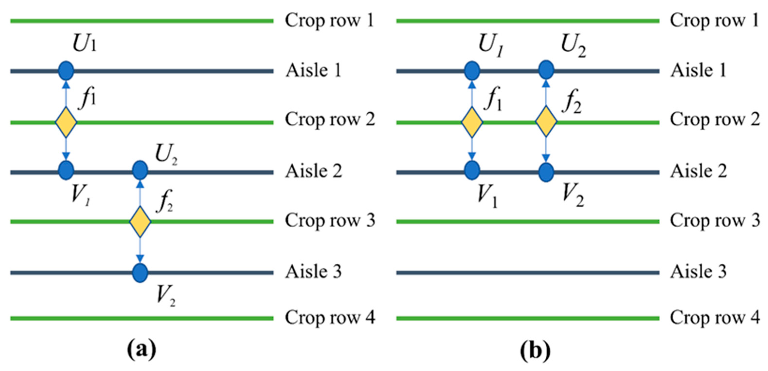
In the detasseling operation, the UDV can remove each male flower from the aisle on both sides of the crop row where the male flower is located. There are two positions where a male flower can be removed. These correspond to the projection nodes located on either side of each male flower, as shown in Figure 3. Before calculation, this study needs to obtain the projection node coordinates of the aisle on both sides of each male flower. One projection node is set as Un, and the other projection node is set as Vn. In subsequent calculations, the names of projection nodes cannot be changed. Compared with the traditional TSP, the difference in this paper is that there are eight different routes between two male flowers.
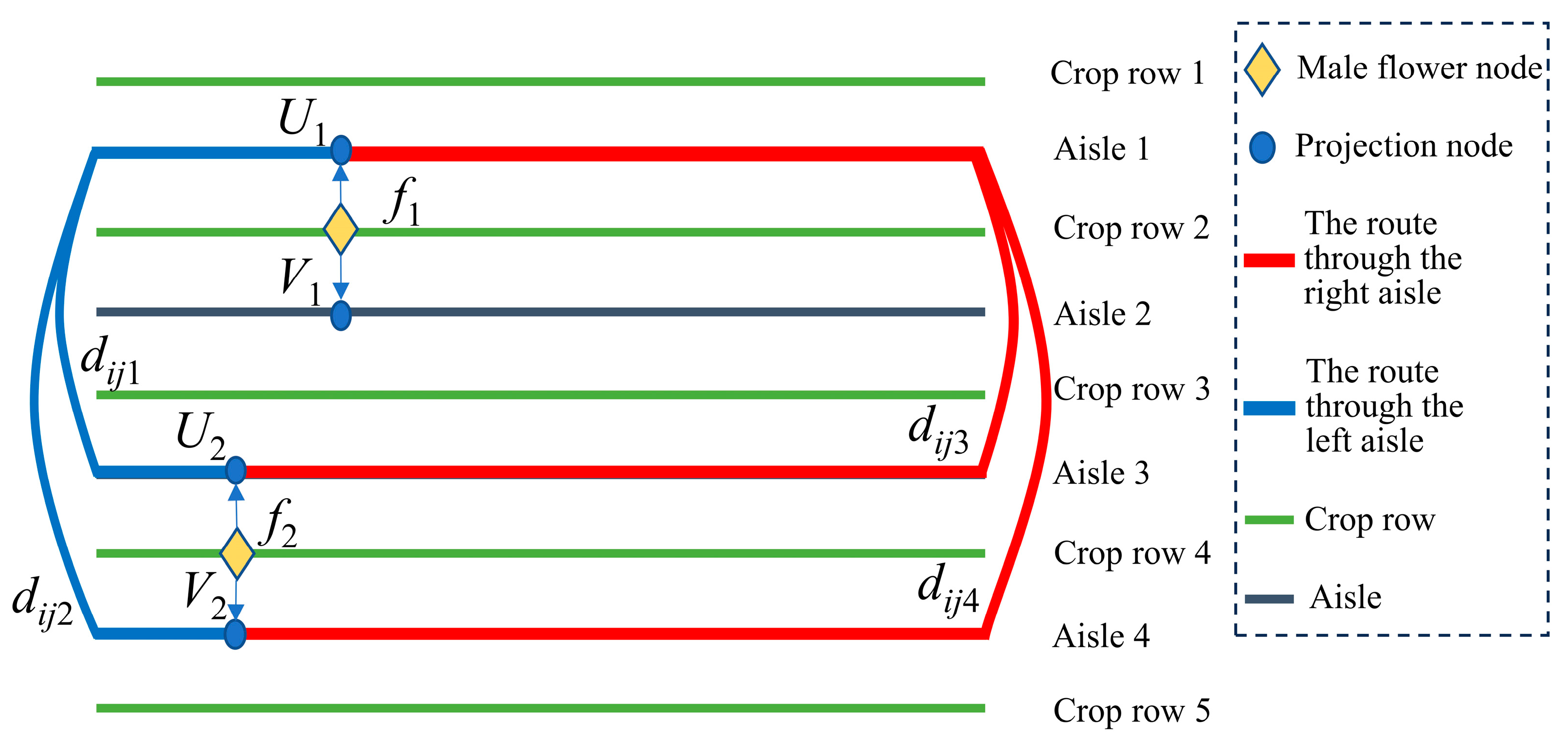
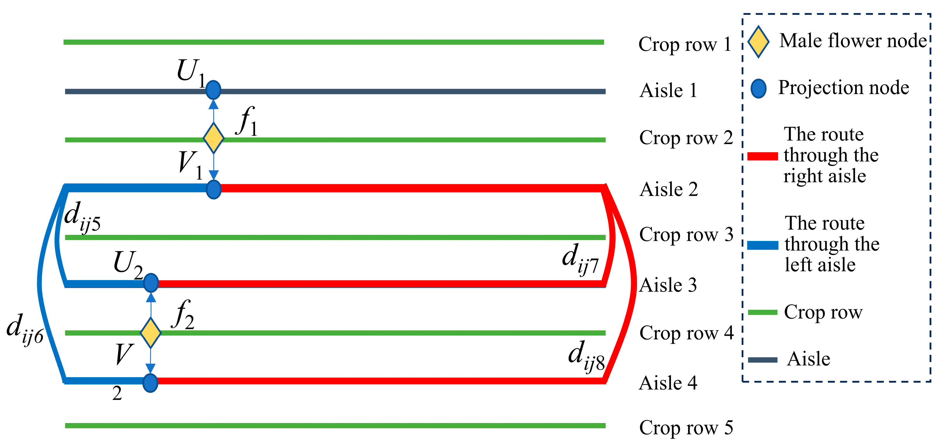
During the route selection process from fi to fj, given that the position of UDV reaching fi has already been determined through the preceding selection process, four potential routes exist from fi to fj. Two of these routes lead to the projection nodes Uj and Vj of fj.
As shown in Figure 3 and Figure 4, if the current position of UDV is at U1 and the next target male flower node is f2, there are four routes between f1 and f2. If the current position of UDV is at V1 and the next target male flower node is f2, then there are still four routes between f1 and f2. The conclusion is that there are eight routes between f1 and f2, which increases the difficulty of the detasseling route planning problem. In Figure 3 and Figure 4, dij1~dij4 are distances of four routes from the projection node U1 to the f2; dij5~dij8 are distances of four routes from the projection node V1 to the f2. In Figure 3 and Figure 4, dij1~dij4 are distances of four routes from the projection node U1 to the f2; dij5~dij8 are distances of four routes from the projection node V1 to the f2.
In addition, two special situations should be considered. The first situation is shown in Figure 5a. The projection node V1 of f1 and the projection node U2 of f2 are located in the same aisle. At this time, there is only one route from V1 to U2, which will make the total number of methods from f1 to f2 become seven. The other situation is shown in Figure 5b, where f1 and f2 are on the same crop row. There are three routes from U1 to f2. Similarly, there are three routes from V1 to f2.
The detasseling sequence and the approach to the male flower should be contained in the output results, which are expressed as follows:
R 1 = r 1 z R 2 = r 2 z
in which R1 denotes the set of sequences for removed male flowers, where each element in the set corresponds to the positional information of a male flower that has been removed. r1z denotes the z-th removed male flower in the sequence, r1z =fn; R2 represents the sequence set of the approach coordinates for removed the male flowers. The elements in the set are the sets of aisle coordinate information. z denotes the detasseling sequence number, z = 1, 2……N; r2z denotes the approach to the z-th removed male flower, its value is shown as follows:
r 2 z = s k   If   UDV   reaches   the   male   flower   from   S k w k   If   UDV   reaches   the   male   flower   from   W k   0   If   UDV   does   not   exit   current   aisle
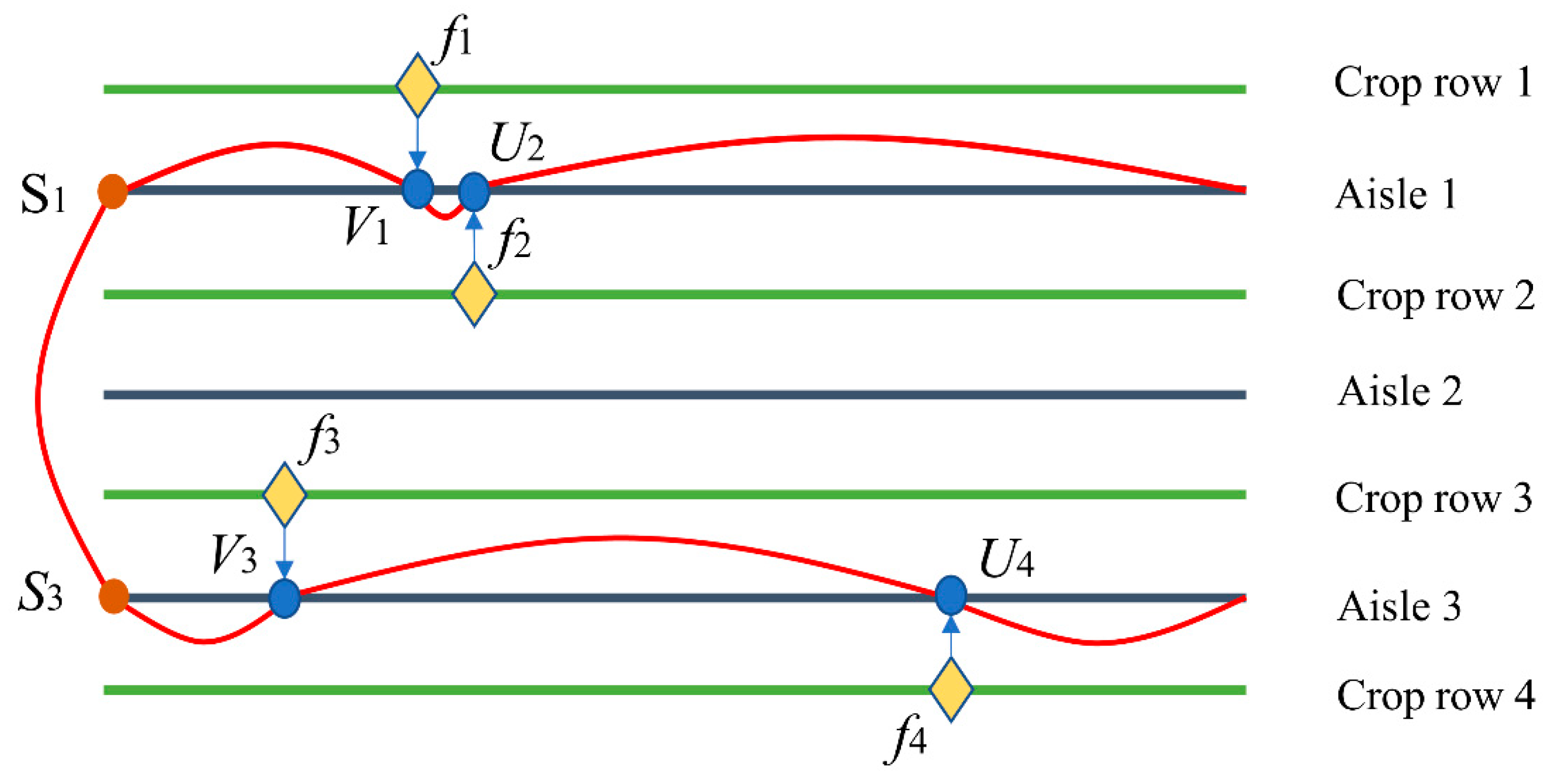
For example, Table 1 lists the output data that documents the UDV’s detasseling operation route for the male flowers f1, f2, f3, f4, and f5. And the specific routes represented by the result are shown in Figure 6. The UDV reaches the male flower f4, after the UDV leaves the endpoint W3. Then, it is defined as the case that the UDV reaches the male flower f4 from the endpoint W3. Therefore, r11 = f4 and r21 = w3 are set corresponding to the case. The UDV reaches the male flower f3, after the UDV leaves the male flower f4. Then, it is defined as the case that the UDV does not exit the current aisle. Therefore, r12 = f3 and r22 = 0 are set corresponding to the case. Next, the UDV passes through the endpoints S3 and S1 to reach the male flower f1. Before the UDV reaches male flower f1, endpoint S1 is the last node it passes through. Then, it is defined as the case that the UDV reaches the male flower f1 from the endpoint S1. Therefore, r13 = f1 and r23 = s1 are set corresponding to the case. Similarly, r14 = f2 and r24 = 0 represent that the UDV reaches male flower f2 from the previous male flower without exiting the current aisle.

2.3. The Objective Function

The detasseling route planning problem in this paper can be described as an optimization problem of finding the shortest route, in which the UDV has to traverse all male flowers. It can be seen from Section 2.2 that there are eight routes and two special situations from the i-th male flower to the j-th male flower. The distances of the eight routes are set as dij1~dij8. Among them, dij1~dij4 are distances of four routes from the projection node Ui to the j-th male flower; dij5~dij8 are distances of four routes from the projection node Vi to the j-th male flower.
Further, dij1 and dij2 are the distances of the UDV starting from projection node Ui, passing through endpoint Sk, to projection node Uj and Vj, respectively. dij3 and dij5 are the distances of the UDV starting from projection node Uj, passing through endpoint Wk, to projection node Uj and Vj, respectively. The difference between dij5~dij8 and dij1~dij4 is that the starting node is different. The starting node of dij5~dij8 is Vi. The distance calculation method of dij1 can be expressed as follows:
d i j 1 = ( x u i x s k i ) 2 + ( y u i y s k i ) 2 + ( x s k i x s k j ) 2 + ( y s k i y s k j ) 2 + ( x u j x s k j ) 2 + ( y u j y s k j ) 2  
in which (xski,yski) denotes the coordinates of the endpoint Ski of the aisle where Ui is located; (xskj,yskj) denotes the coordinates of the endpoint Skj of the aisle where Uj is located; (xui,yui) and (xuj,yuj)denotes the coordinates of Ui and Uj.
The calculation method of dij2……dij8 is similar to the calculation method of dij1.
For the two special situations mentioned in Section 2.2, in the first situation, the dij5 = dij7, the calculation method can be expressed as follows:
d i j 5 = d i j 7 = ( x v i x u j ) 2 + ( y v i y u j ) 2
In the second special situation, the dij1 = dij3, dij6 = dij8, the calculation method of dij1 and dij3 can be expressed as follows:
d i j 1 = d i j 3 = ( x u i x u j ) 2 + ( y u i y u j ) 2
The calculation method of dij6 and dij8 can be expressed as follows:
d i j 6 = d i j 8 = ( x v i x v j ) 2 + ( y v i y v j ) 2
In order to facilitate the construction of the objective function, the decision variable εijp is set. The decision variable is shown as follows:
ε i j p = 1   if   d i j p   is   in   the   current   result 0   otherwise
in which p = 1, 2…8.
The objective function of the problem is shown as follows:
min l = i = 1 N j = 1 N p = 1 8 ε i j p d i j p
in which l denotes the detasseling operation distance.

2.4. Establishment of Polygonal Boundary Field Model

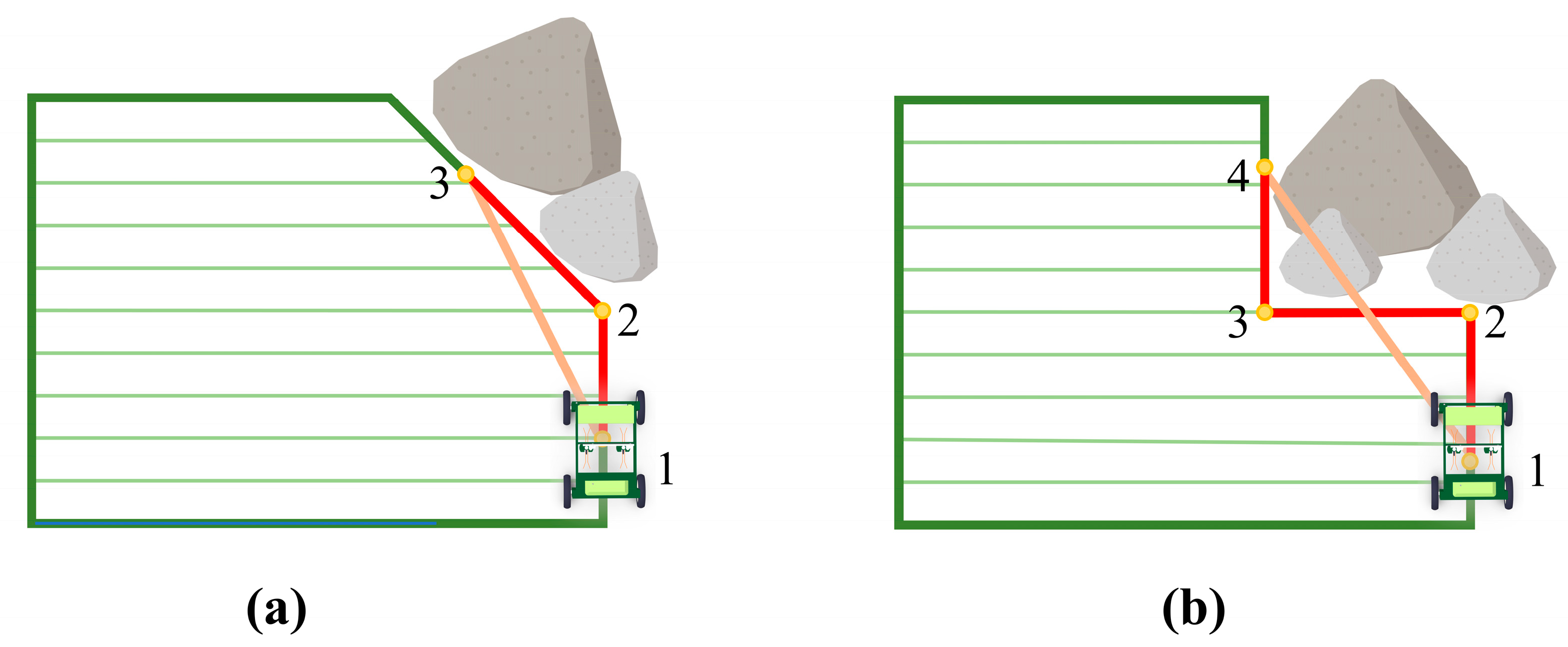
In the actual situation, in addition to the rectangular field plots, there are also fields with polygonal boundaries. For fields with polygonal boundaries, the distance calculations in the matrix for male flower nodes need adjustment. This mainly includes the two cases shown in Figure 7.
The field plot shown in Figure 7a has a convex polygon boundary. In the figure, aisle endpoints 1 and 2 are on the same vertical side. The operation route passes through aisle endpoints 1 and 2, and the distance calculation uses Equation (14).
dist 2 ( 1 , 2 ) = ( x 1 x 2 ) 2 + ( y 1 y 2 ) 2
in which dist2(1, 2) denotes the Euclidean distance between endpoint 1 and endpoint 2. Aisle endpoints 2 and 3 are on the same inclined side. The route goes through these endpoints. Distance calculation uses Equation (15).
dist 2 ( 2 , 3 ) = ( x 2 x 3 ) 2 + ( y 2 y 3 ) 2
in which dist2(2, 3) denotes the Euclidean distance between endpoint 2 and endpoint 3. Aisle endpoints 1 and 3 are located on different sides. To avoid damaging the crops, the operational route connecting aisle endpoints 1 and 3 cannot directly follow the straight-line segment. Instead, it must traverse through aisle endpoints 1, 2, and 3 in sequence. The calculation of the distance L13 between aisle endpoints 1 and 3 is based on arithmetic Formula (16).
L 13 = dist 2 ( 1 , 2 ) + dist 2 ( 2 , 3 )
Figure 7b shows a field plot with a concave polygon boundary, typically formed to avoid obstacles. One particular situation in the figure is that aisle endpoints 1 and 4 are on opposite sides. Since crossing through fields or obstacles is not allowed, the route between aisle endpoints 1 and 4 must pass sequentially through aisle endpoints 1, 2, 3, and 4. The distance L14 between aisle endpoints 1 and 4 is calculated using arithmetic Formula (17).
L 14 = dist 2 ( 1 , 2 ) + dist 2 ( 2 , 3 ) + dist 2 ( 3 , 4 )

3. The Proposed DRDM-AACO

In this paper, ACO is used to deal with the route planning problem due to its applicability to the TSP. However, the traditional ACO algorithm only takes into account the Euclidean distance of a single route between nodes. In contrast, in real farmland environments, multiple feasible routes exist between male flower nodes, which are constrained by crop rows. In addition, the distribution of male flower nodes in the field has a hybrid spatial characteristic, including a two-dimensional distribution across different crop rows and a one-dimensional distribution along the same crop row. Moreover, the UDV has detailed requirements, such as a double-row working width, which further complicates the issue. Therefore, traditional ACO must be improved to solve this heterogeneous TSP with hybrid space constraints. In response to the above issues, four mechanisms are proposed in the following text.

3.1. Dual-Route Preference Mechanism

There are eight routes between each pair of male flower nodes, requiring eight distance matrices. As shown in Figure 3 and Figure 4, there are eight possible routes between male flowers fi and fj. In the selection results, only changes in Uj and Vj will influence subsequent route selection, thereby impacting the overall routing outcome.
Therefore, to simplify the calculation, only the shortest routes to the projection nodes Uj and Vj of fj are retained. Among them, the shorter route is named the main route, and the other one is named the auxiliary route. The dual-route preference mechanism involves the establishment of heuristic information and the establishment of a dual-route collaborative probability decision model.

3.1.1. Heuristic Information of the Dual-Route Preference Mechanism

Heuristic information is related to the distance matrix and will affect the selection probability. In traditional ACO, there is only one route between the current node and the target node, so there is only one heuristic information.
Based on the dual-route preference mechanism, when the UDV is positioned at the projection node Ui or Vi of the current male flower node fi and selects the subsequent male flower node fj, two critical routes are involved in this selection process: the main route and the auxiliary route.
d i j u main = min d i j 1 , d i j 3 , d i j 2 , d i j 4
d i j u aux = max min d i j 1 , d i j 3 , min d i j 2 , d i j 4
d i j main = d i j u main ,     if   UDV   is   at   U i d i j v main ,     if   UDV   is   at   V i
d i j aux = d i j u aux ,     if   UDV   is   at   U i d i j v aux ,     if   UDV   is   at   V i
In which d iju   main denotes the main route distance from the projection node Ui of fi to fj, and d iju   aux denotes the auxiliary route distance from the projection node Ui of fi to fj. In the same way, d ijv   main denotes the main route distance from the projection node Vi of fi to fj, and d i j v   aux denotes the auxiliary route distance from the projection node Vi of fi to fj. d ij   main represents the main route distance from male flower fi to male flower fj, and d ij   aux represents the auxiliary route distance from male flower fi to male flower fj.
In which D u main is the main route distance matrix between the projection node Un and the target male flower node, and D u aux is the auxiliary route distance matrix between the projection node Un and the target male flower node. As well, the main and auxiliary route matrices between the lower projection point Vn and the target male flower node are, respectively, denoted by symbols D v main and D v aux , and their solution processes are similar to Equations (18) and (19).
In accordance with the distance matrix, the heuristic information matrix denotes can be formulated as follows:
η i j u main = 1 / d i j u main
η i j u aux = 1 / d i j u aux
η i j main = η i j u main ,     if   UDV   is   at   U i η i j v main ,     if   UDV   is   at   V i
η i j aux = η i j u aux ,     if   UDV   is   at   U i η i j v aux ,     if   UDV   is   at   V i
η iju   main denotes the main route heuristic information from the projection node Ui on fi to fj, and η iju   aux denotes the auxiliary route heuristic information from the projection node Ui on fi to fj. η ijv   main and η ijv   aux are defined in the same way. η ij   main denotes the main route heuristic information from male flower fi to male flower fj, and η ij   aux denotes the auxiliary route heuristic information from male flower fi to male flower fj.

3.1.2. Dual-Route Collaborative Probability Model

To address the slow convergence and low route quality in traditional ACO for maize detasseling operation routes, a dual-route collaborative probability decision model is proposed. This model transforms single-route probability calculations into dual-route calculations by combining the probabilities of both routes into the total probability for selecting the next male flower node.
The probability P ij   m that the m-th UDV travels from male flower node fi to node fj is calculated as follows:
P i j m = [ τ i j main ( t ) ] α ( η i j main ) β + [ τ i j aux ( t ) ] α ( η i j aux ) β s O i m [ τ i s main ( t ) ] α ( η i s main ) β + [ τ i s aux ( t ) ] α ( η i s aux ) β
In which τ ij   main denotes the pheromone concentration on the main route d ij   main at the t-th iteration. τ ij   aux denotes the pheromone concentration on the auxiliary route d ij   aux at the t-th iteration. O i   m denotes the candidate set when the m-th UDV is at the male flower node fi. α is the pheromone importance factor; β is the heuristic function importance factor.
P ij   m includes two terms. The first term denotes the probability of transitioning from male flower node fi to fj through the main route, and the second term denotes the probability through the auxiliary route.
The dual-route collaborative probability decision model, based on the dual-route preference mechanism, removes the longer route between two male flower nodes. This reduces the number of routes for selection and improves the quality of the remaining routes. Additionally, since the endpoints of the main and auxiliary routes include projection nodes Uj and Vj of the male flower node fj, the starting nodes for subsequent selection remain unaffected, preserving the route topology integrity.

3.2. Dynamic Candidate Set

When the model includes many male flower nodes, the ant colony algorithm’s runtime becomes too long. Experiments show that in better solutions, the row difference between consecutively removed male flower nodes is usually 0 to 3. Based on this, a dynamic candidate set mechanism was proposed.
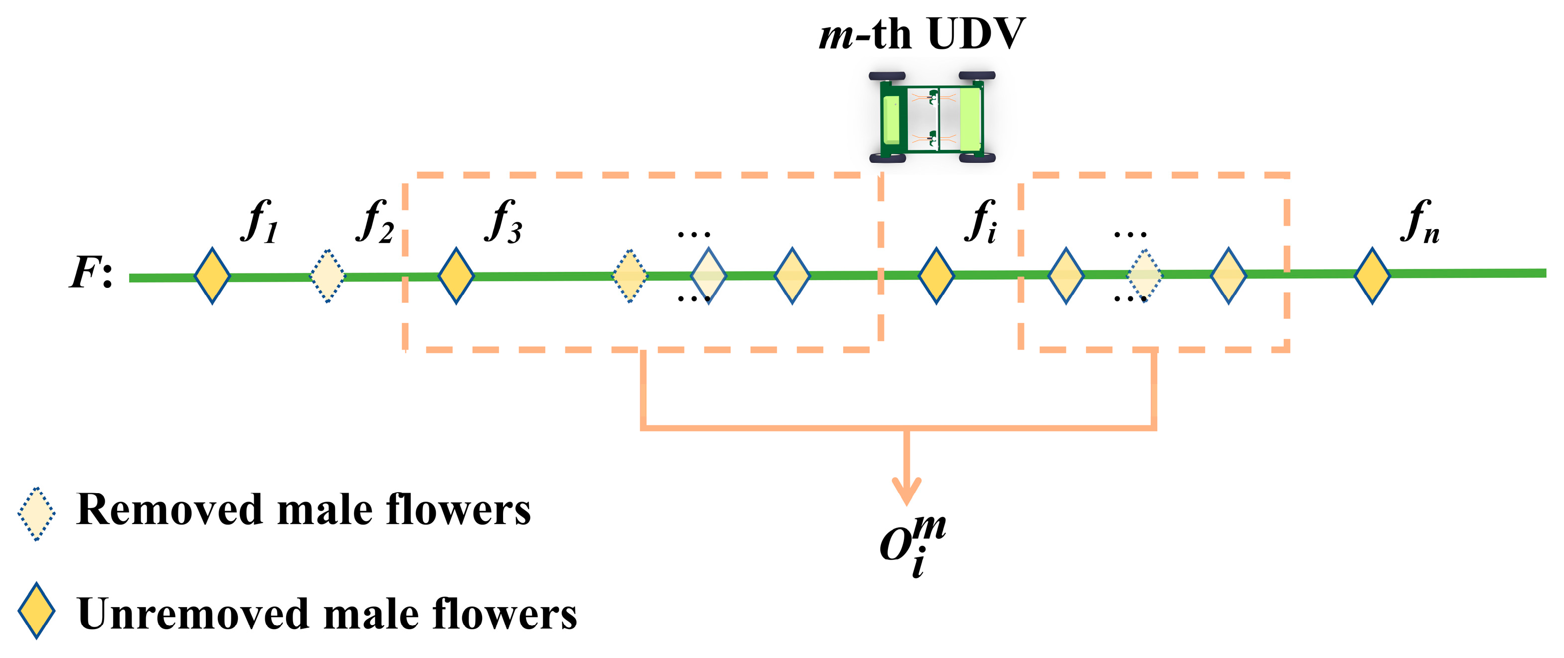
As shown in Figure 8, the dynamic candidate set is constructed as follows: when the m-th UDV is at male flower node fi, a subset of adjacent male flower nodes is selected to form O i   m . To construct O i   m , consider the following:
Firstly, the male flower nodes that have already been removed should be excluded from the candidate set O i   m , as shown by the dashed diamonds in Figure 8.
Secondly, the candidate set O i   m is dynamic, adapting based on the position of fi rather than simply removing eliminated nodes as in traditional ACO.
In addition, it should be noted that the depiction of all male flower nodes in Figure 8, located on a single crop row, is an abstract representation. In reality, male flower nodes may be distributed across different crop rows. By applying these principles, the size of O i   m is significantly reduced compared to traditional methods, decreasing runtime without compromising optimization quality, as the retained nodes are more likely to produce better routes.
The dynamic candidate set O i   m is defined as follows:
O i m = F T i m
O i m = φ F T i m
φ = φ 0 exp 0.6 × ( t 1 ) / T
O i   m   denotes the number of selectable male flowers in the dynamic candidate set. T i   m denotes the set of taboo tables, which represents the set of positional coordinates of the traversed male flowers. φ denotes the scale ratio coefficient, with a range of [0, 1], and φ0 denotes the basic scale ratio coefficient.
The dynamic candidate set   O i   m varies with the position of the male flower node fi and continuously decreases as t increases. This approach ensures global optimization initially, improves convergence later, and reduces runtime.

3.3. Non-Uniform Initial Pheromone Allocation

In the traditional ant colony optimization, the initial pheromone is usually uniformly distributed. This strategy neglects the spatial distribution characteristics of the male flower nodes located in the crop rows in the field, as well as the route constraints and working width conditions of the UDV movement. This leads to many ineffective cross-row searches in the early stage.
For this issue, this study proposes a non-uniform initial pheromone allocation mechanism based on the spatial distribution characteristics of male flower nodes and the intra-row and inter-row coupled constraints. Through inter-row and intra-row collaborative constraints, the algorithm reduces cross-row searches and enhances intra-row routes. An exponential function suppresses cross-row search and assigns multiple pheromone weights to nodes in the same row. This method can prioritize continuous intra-row routes and reduce energy consumption from turnback.
τ i j ( 0 ) = τ 0 e γ | r i r j | 1 + η δ same ( i , j ) 1 1 + d i j / d max
δ same ( i , j ) = 1 ,       if   f i   and   f j   at   the   same   aisle 0 ,       otherwise
τ0 represents the initial pheromone factor, and its value is 1. γ represents the inter-row attenuation coefficient, while η represents the intra-row enhancement factor. The function δsame(i, j) denotes the same row indicator function. It takes the value of 1 when any projection node of the male flower nodes fi and fj are in the same row of the aisle, and zero otherwise. dij represents the distance from the male flower node fi to fj, including both the main route and the auxiliary route distances; dmax represents the distance of the longest route from male flower node fi to fj.
The first term in Equation (28) is the inter-row attenuation term, which suppresses the generation of redundant cross-row routes. The second term is the intra-row enhancement term, which increases the connection probability of intra-row male flower nodes to achieve continuous operation of UDV. The third term is the distance penalty term, which takes into account the influence of the distance between male flower nodes.

3.4. Direction-Constrained Adaptive Dual-Model Pheromone Regulation

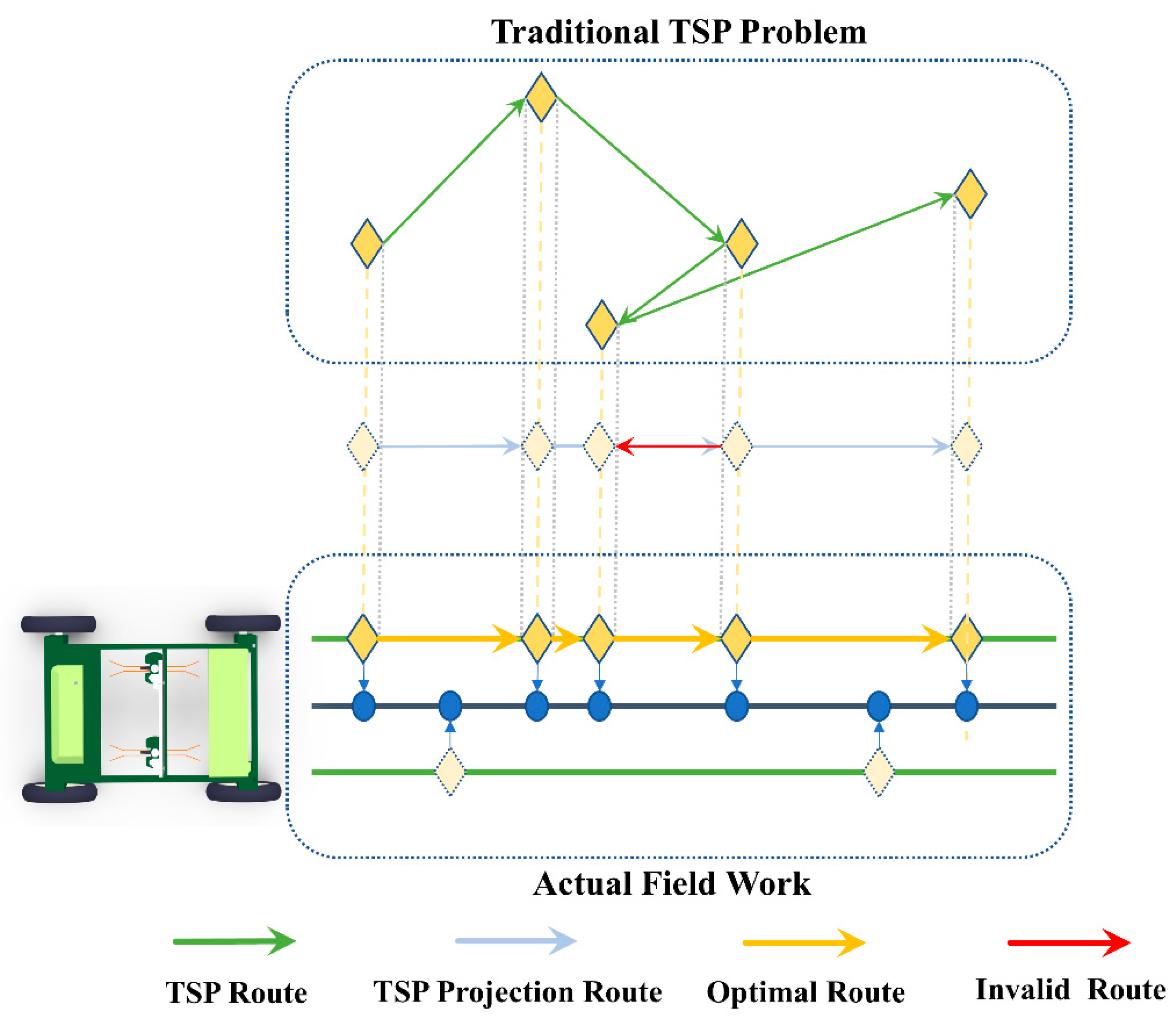
In the traditional TSP model, routes can extend freely without considering intersection or turnback issues, as shown in Figure 9. However, maize plants are planted in crop rows, which makes the routes between some male flower nodes have one-dimensional characteristics. This demands that UDV operation routes sequentially traverse the projection nodes of male flowers to avoid unnecessary intra-row turnback routes. In contrast, the traditional TSP model distributes nodes in a two-dimensional space, avoiding obvious turnback routes. When male flower nodes are on the same crop row, or their projection points align in the same aisle across different crop rows, obvious turnback routes occur, increasing the total route length.
To address the issue of ineffective turnback routes in traditional ACO for route planning in detasseling operations, this study proposes a direction-constrained adaptive dual-mode pheromone regulation mechanism. This mechanism optimizes intra-row route continuity by combining local penalty and global dynamic evaporation, suppressing intra-row turnback routes.
In the local penalty mode, if the UDV generates a turnback route in the same aisle row, the pheromone deposition amount on this route is penalized to suppress future deposition. The improved pheromone increment Δ τ ij m t , is calculated as follows:
Δ τ i j m ( t ) = Q l m ( t ) ζ Q d i j ,     ( i , j ) r 1 z m ( t ) , r 1 z + 1 m ( t ) 0 ,                                                   otherwise
Δ τ ij m t denotes the pheromone increment on the route of dij from the m-th ant in the iteration t, including the pheromone on the main route and the pheromone on the auxiliary route. ζ denotes the turnback penalty factor, which takes values in the range [0, 1]. dij denotes the intra-row turnback route distance between fi and fj, either the main or auxiliary route. Q denotes the pheromone intensity value.
Under the dynamic global evaporation mode, the pheromone evaporation process is supplemented with an adaptive evaporation coefficient ρ(t). This coefficient adaptively modulates the evaporation intensity according to the ratio of intra-row turnback routes to the total number of movements. Consequently, this mechanism further enhances the evaporation rate of intra-row turnback routes, thereby facilitating faster convergence toward a more optimal route solution. The improved pheromone update method is as follows:
τ i j ( t + 1 ) = [ 1 ρ ( t ) ] τ i j ( t ) + m = 1 M Δ τ i j m ( t )
ρ ( t ) = ρ 0 + λ N num N total ,     if   intra   -   row   turnback   route ρ 0 ,                                               if   intra   -   row   forward   route
ρ0 denotes the basic pheromone evaporation coefficient; λ denotes the adjustment coefficient, which controls the sensitivity to the intra-row turnback route. λ = 0 when the route is the forward route, λ ≠ 0 when it is the intra-row turnback route. Nturn denotes the number of intra-row turnback routes; Ntotal denotes the total number of movements.

3.5. Improved ACO Workflow

This section mainly introduces the programming methods and realization approach of DRDM-AACO. To easily facilitate development across different software platforms, we systematically summarize the corresponding pseudocode in Table 2.
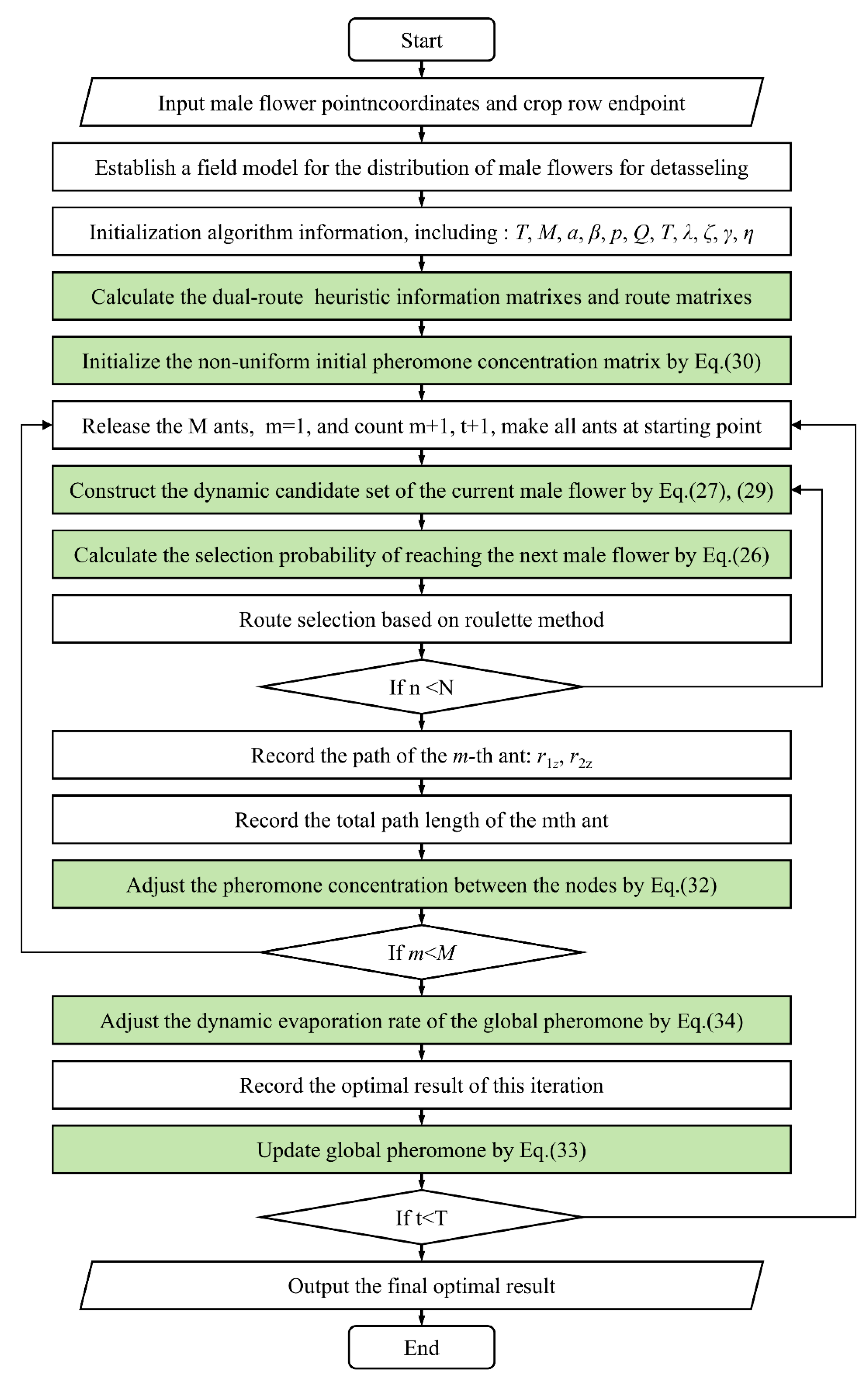
In Figure 10, the flowchart illustrates the realization process of DRDM-AACO. The green-filled boxes in the figure highlight the differences between DRDM-AACO and the traditional ACO algorithm.

4. Results

4.1. Performance Verification of the Four Proposed Improvements

To test and distinguish the effectiveness of each proposed improvement, the four mechanisms are combined with traditional ACO sequentially. Thus, several transitional variants of ACO are formed. For convenience, these transitional variants are simply named as ACO-1, ACO-2 and ACO-3 as shown in Table 3. After integrating all the four improvements with traditional ACO, the final variant of ACO is called DRDM-AACO (Dual-Route and Dual-Mode Adaptive Ant Colony Optimization).
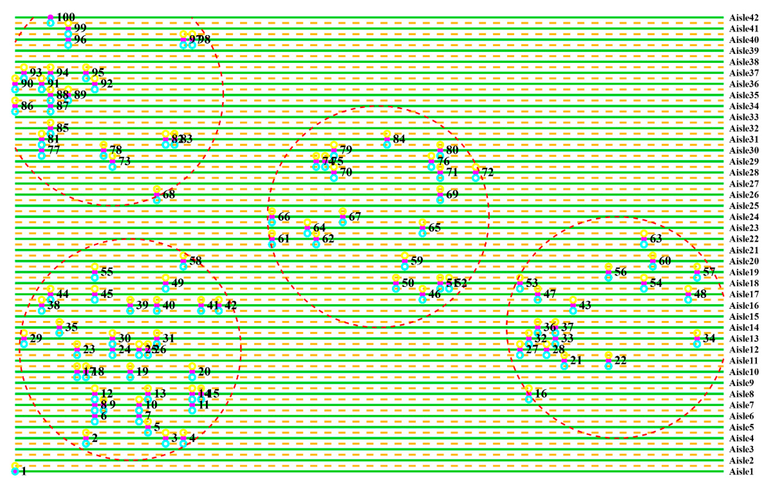
Rectangular fields are the most fundamental working environment for maize detasseling operations, used to test the performance of each improvement. The field model setting is shown in Figure 11. In the model, the area of the rectangular field is one mu. “Mu” is a traditional Chinese unit of land area measurement. Considering the maize planting spacing requirements set in this paper, the size of the one mu field is set to 32 m × 20.5 m. Plants were spaced 0.5 m apart between rows and 0.4 m within rows, with a total of 42 rows in the rectangular field. The row ratio of female to male maize plants is set at 5:1 to meet the agronomic requirements for maize seed production fields. To investigate the applicability of the improved Ant Colony Optimization (ACO) algorithm, the number of male flowers was set to 100, 150, and 200. Due to the non-uniform distribution of sunlight, water, and fertilizer across the field, the growth rate of male flowers varies significantly among different regions. To simulate this phenomenon, the model assumes plants requiring detasseling are located in distinct circular zones. To simplify the description, the task of detasseling 100 male flowers per mu is abbreviated as N1F100, and 200 male flowers per mu as N1F200, and so on.
The IDAACO proposed by Liu et al. adopts the heuristic strategy with direction information, adaptive pseudorandom transfer strategy, improved local pheromone updating mechanism and improved global pheromone updating mechanism [29]. These strategies have adaptive regulation characteristics for various parameters and are mainstream improvement methods. In this study, IDAACO was simply improved based on maize detasseling characteristics, and a dual-route optimization mechanism was added to align it with the problem model. A comparative experiment was then conducted between IDAACO and DRDM-AACO.
During the experiment, the parameter settings of all ACO variants, including DRDM-AACO and IDAACO, are shown in Table 4.
Intelligent algorithms generate solutions that may be better or worse than previous results due to randomness. Therefore, in this section, each algorithm is independently run 20 times. The experimental results of the five algorithms are shown in Table 5.
In maize detasseling route planning, improved algorithm performance is crucial. Experimental data in Table 5 show that the DRDM-AACO outperforms the traditional ACO algorithm. For example, in the N1F200 scene, DRDM-AACO achieves an optimal route length of 541.45 m (6.01% shorter than ACO’s 576.05 m) and an average route length of 545.05 m (6.12% shorter than ACO’s 580.60 m).
In Table 5, As the number of male flower nodes increases, the average runtime of the program also increases. From the pseudocode of DRDM-AACO in Table 2, we can derive the time complexity of the program: when constructing a complete route for a single ant, the time complexity scales as O(N2) with the number of nodes. N represents the number of male flower nodes. Given M ants and T iterations, the overall time complexity is O(T·M·N2), where T and M are algorithmic parameters, which the number of iterations and the number of ants, respectively, are set as constants typically. Thus, the algorithm’s runtime exhibits quadratic polynomial growth relative to the number of male flower nodes N, specifically O(N2).
To understand the improvement mechanism of the DRDM-AACO, this paper sequentially introduces each mechanism into the ACO algorithm, conducts experiments, and analyses the impact based on the results.
The dual-route optimization mechanism is discussed by comparing ACO with ACO-1. Through experimental data, it was found that the total distance of ACO-1 is shorter compared with ACO. For example, in the N1F100 scene, the average route length of ACO-1 was reduced by 2.2% compared to ACO (504.47 m → 493.35 m), and the optimal route length decreased from 496.75 m to 491.65 m. In this example, while the optimization outcome of ACO-1 is superior, the improvement relative to the optimization result of ACO is relatively modest. This is primarily attributed to the low density and quantity of male flower nodes, which in turn reduces the complexity of the task and limits the options for route selection. In the scene of high-density male flower nodes, the reduction in the optimization results of ACO-1 compared to ACO increases.
In the N1F150 scene, the average route length for ACO-1 was reduced by 1.96% compared to ACO (595.80 m → 584.13 m), while the optimal route length decreased from 587.85 m to 582.25 m. In the N1F200 scene, the average route length for ACO-1 was reduced by 3.03% compared to ACO (581.20 m → 563.60 m), while the optimal route distance decreased from 576.05 m to 559.05 m. Experimental data shows that the dual-route preference mechanism leads to shorter optimization results by maintaining both main and auxiliary routes between nodes. The dual-route preference mechanism increases the diversity of candidate routes and ensures the topological features of the complete global optimal route. Thus, this method prevents the algorithm from getting trapped in local optimal solutions and improves the quality of the optimization results. In order to facilitate the expression of the analysis content, in the subsequent analysis content, the detasseling sequence number of the male flower nodes labeled in the route map of the calculation results is used as the male flower node number fn.
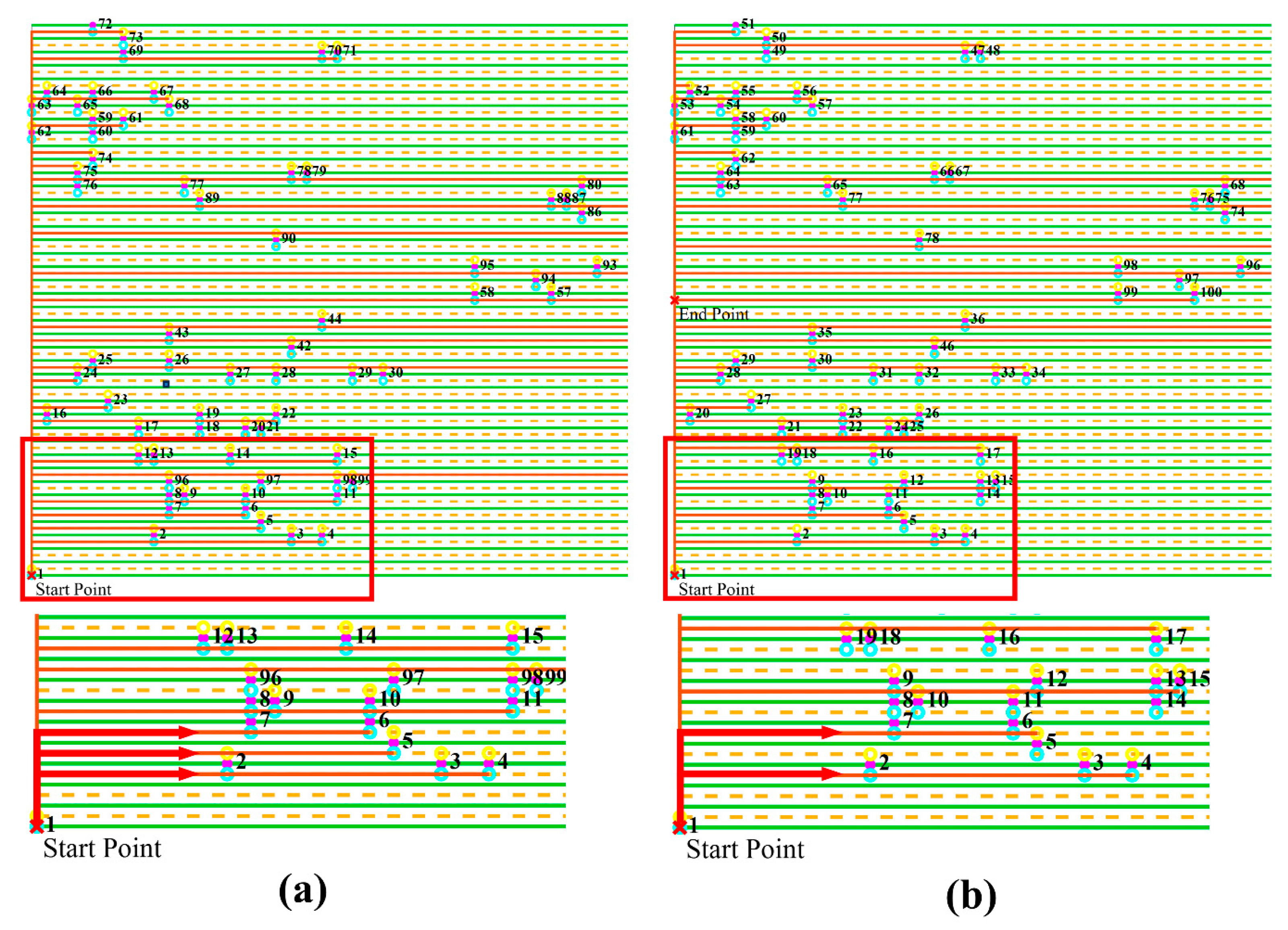
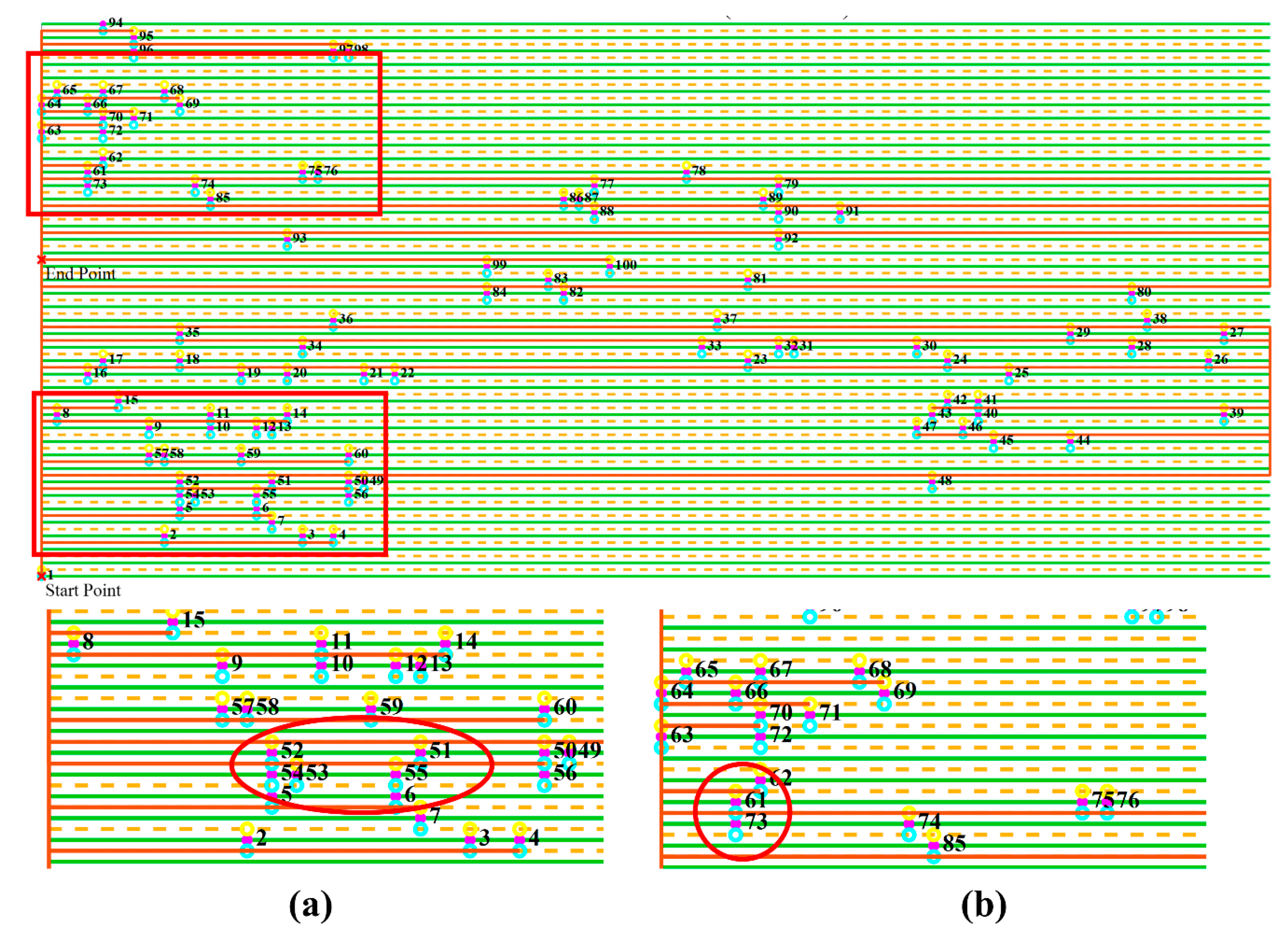
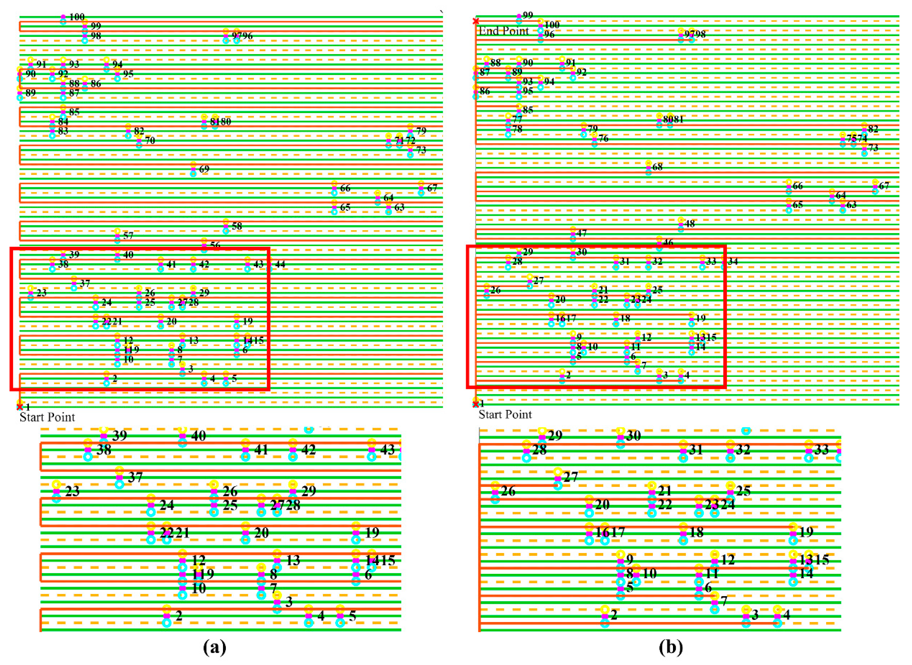
Figure 12a shows that in the optimization results, ACO retains the shortest routes from f4 to f5 and from f5 to f6, that is, from V4 to V5 and from V5 to V6, and its optimization result is V4V5V6. As for f4 to f5, ACO-1, as shown in Figure 12b, retains two routes from V4 to V5 and from V4 to U5, increasing the diversity of candidate routes, making its optimization result possibly V4U5V6. Although the distance from V4 to U5 is longer than that from V4 to V5, the total distance of V4U5V6 is shorter than that of V4V5V6.
The discussion between ACO-1 and ACO-2 focuses on the dynamic candidate set mechanism. The data in Table 5 indicate that ACO-1 requires more runtime than ACO-2 due to its dual-route preference mechanism, which retains both main and auxiliary routes. ACO-2 is an algorithm constructed based on ACO-1 by introducing the dynamic candidate set mechanism, aiming to improve the computational efficiency of the algorithm while also considering the quality of the calculation results.
The data in Table 5. Abbreviation for the variants of ACO, DRDM-AACO, IDAACO. shows that in the N1F200 scene, the average runtime of ACO-2 is 48.61% less than that of ACO-1 (244.45 s → 125.63 s), and the optimization results remain basically the same. In the N1F100 and N1F150 scenes, compared with ACO-1, ACO-2 not only has a shorter computing time but also a shorter optimal route length. The above experimental data indicate that the dynamic candidate set mechanism significantly improves the computing efficiency by compressing the scale of neighborhood nodes. At the same time, the reduction in the search space does not have an adverse effect on the algorithm’s optimization ability, which also verifies that the dynamic candidate set mechanism proposed in this paper is a dynamic pruning of invalid nodes based on the characteristics of the maize seed production field detasseling operation problem.
The size of the dynamic candidate set determines the number of nodes to be selected at each decision node, and the scale ratio coefficient φ constitutes a core parameter in the dynamic candidate set mechanism. Therefore, a detailed discussion regarding the basic scale ratio coefficient φ0 is presented to provide a rational and systematic approach for setting this parameter. Taking the N1F150 scene as an example, experiments were conducted with φ0 values ranging from 0.1 to 0.5, and each φ0 value was run 20 times. To demonstrate the algorithm’s optimization performance for different φ0 values, φ = 1 is used as the reference case. For φ = 1, the candidate set size equals the total number of remaining male flower nodes, the route distance is 567.85 m, and the runtime is 117.49 s.
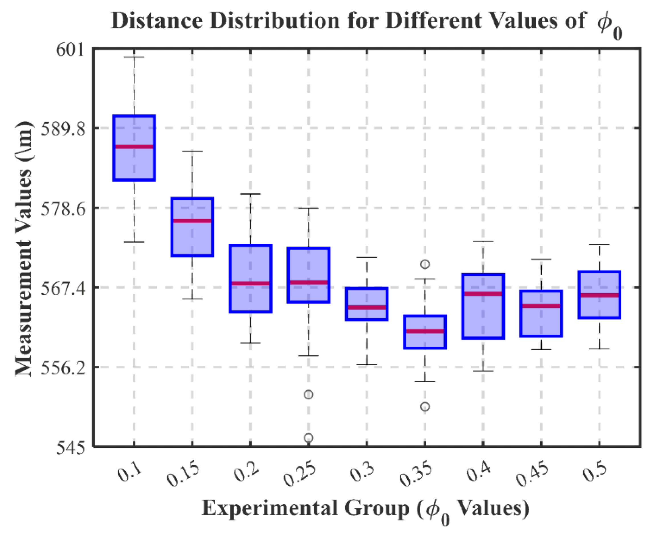
The data in Table 6 shows that the basic scale ratio coefficient φ0 correlates nonlinearly with the total length of the optimized route. This trend is illustrated in Figure 13.
As shown in Figure 13, when φ0 is below 0.35, the total length of the algorithm’s optimization route decreases as φ0 increases. However, when φ0 exceeds 0.35, this trend reverses. Figure 13 shows that within φ0 = 0.3~0.35, the total route length distribution is most concentrated (IQR = 4.2 m), indicating excellent stability. In other ranges, particularly when φ0 < 0.3, the optimization results are less concentrated, with larger differences between upper and lower limits. At φ0 = 0.25, an optimal value of 546.25 m occurs, though the median remains high. The data in Table 6 shows that as φ0 decreases, the algorithm’s runtime progressively reduces. Therefore, considering both the algorithm’s optimization quality and runtime, φ0 is set between 0.3 and 0.45. The algorithm achieves a total length optimization rate exceeding 0.5% and a runtime optimization rate exceeding 34%. φ0 = 0.35 represents the optimal balance between route quality and computational efficiency, with a 1.19% quality improvement and a 41.16% increase in operational efficiency. This value can guide the setting of the basic scale ratio coefficient φ0 for the algorithm.
Next, the discussion between ACO-3 and ACO-2 focuses on the impact of the non-uniform initial pheromone allocation mechanism. The results show that this mechanism sets the initial pheromone concentration based on the distance between male flower points and their row differences, guiding UDV to prioritize exploring potential optimal areas. For example, in N1F100, ACO-3 reduces the average route length by 2.9% compared to ACO-2 (494.45 m → 480.29 m). In N1F150, the reduction is 2.3% (583.60 m → 570.33 m). However, in N1F200, ACO-3 shows similar results to ACO-2, indicating less benefit from non-uniform pheromone allocation in high-density scenes. The discussion compares DRDM-AACO and ACO-3, focusing on the direction-constrained adaptive dual-mode pheromone regulation mechanism. In N1F100, DRDM-AACO reduces the average route length by 3.0% (480.29 m → 465.77 m) and the optimal route length by 3.4% (479.35 m → 462.85 m). In N1F150, the average route length is reduced by 1.4% (570.33 m → 562.37 m) and the optimal route length by 1.6% (568.15 m → 558.95 m). In N1F200, the average route length is reduced by 3.3% (563.37 m → 545.05 m) and the optimal route length by 3.0% (558.05 m → 541.45 m).
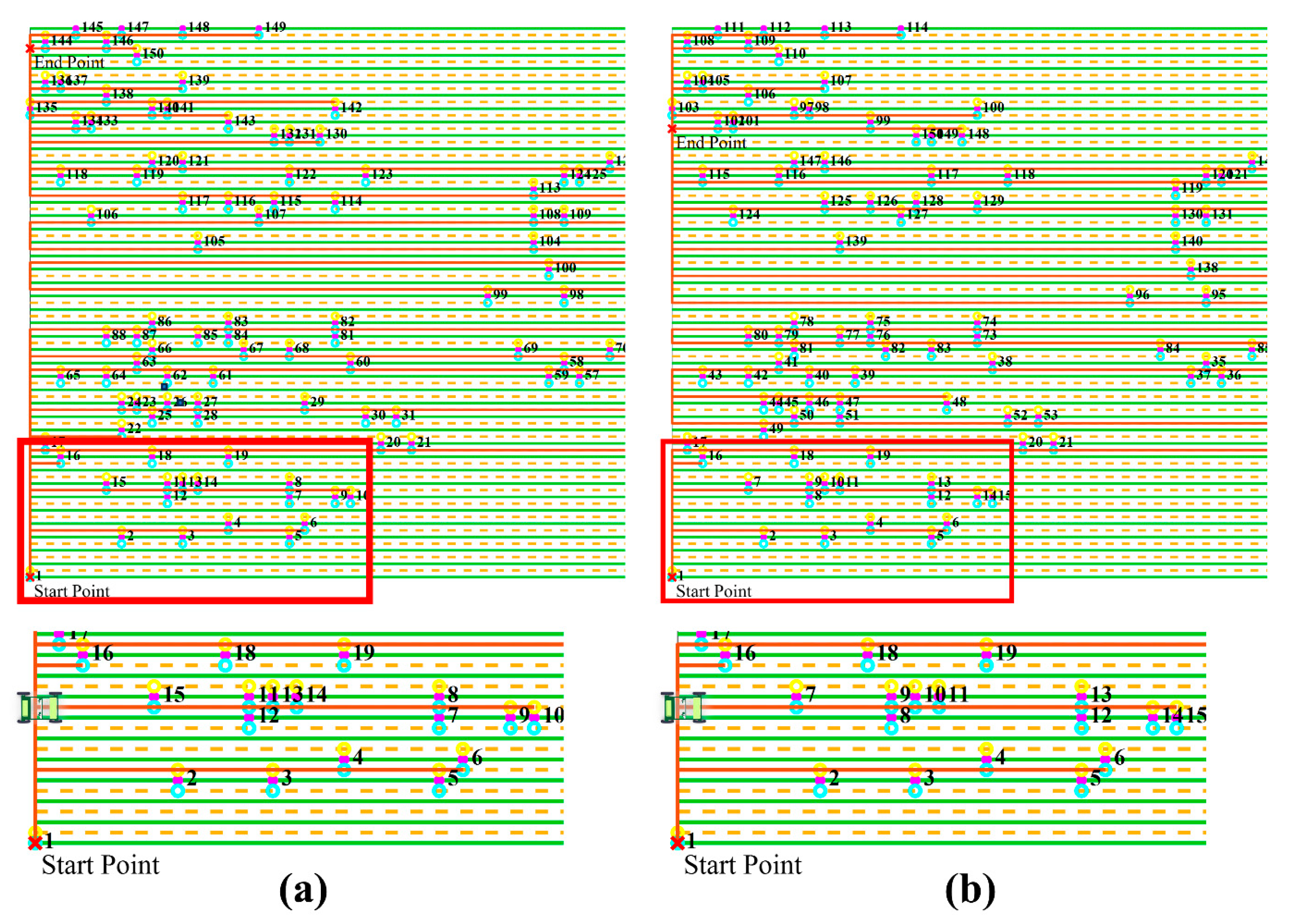
By comparing DRDM-AACO with ACO-3, the direction-constrained adaptive dual-mode pheromone regulation mechanism is shown to enhance optimization by adaptively adjusting the evaporation rate. This mechanism effectively suppresses backtracking routes, as shown in Figure 14a. Results of ACO-3 include a route returning from f10 to f11, f12, and f13, due to small distance differences between nodes leading to similar selection probabilities and many intra-row turnback routes. In contrast, as shown in Figure 14b, DRDM-AACO produces a route from f9 to f10 and then to f11 without intra-row turnback routes. Experimental data further confirms that this mechanism does not significantly increase runtime for DRDM-AACO.
After discussing all the mechanisms of the algorithm, to further verify the overall performance of all the mechanisms of the algorithm, the DRDM-AACO was compared with the IDAACO algorithm proposed by Liu et al. [29]. Through the comparison, it was found that the DRDM-AACO had a shorter optimization result and a shorter runtime. For example, in the N1F150 scene, the average route length of the DRDM-AACO optimization was 562.57 m, which was 4.56% shorter than the IDAACO optimization result. The DRDM-AACO took 64.02 s, which was much lower than the 109.2 s taken by the IDAACO algorithm. Because the IDAACO algorithm does not have the direction-constrained adaptive dual-mode pheromone regulation mechanism proposed in this paper, problems such as intra-row return and multi-row search in the route results are common, as shown in Figure 15a,b, which leads to a longer total route distance.

4.2. Practical Applications

4.2.1. The Establishment of the Kinematic Model of UDV

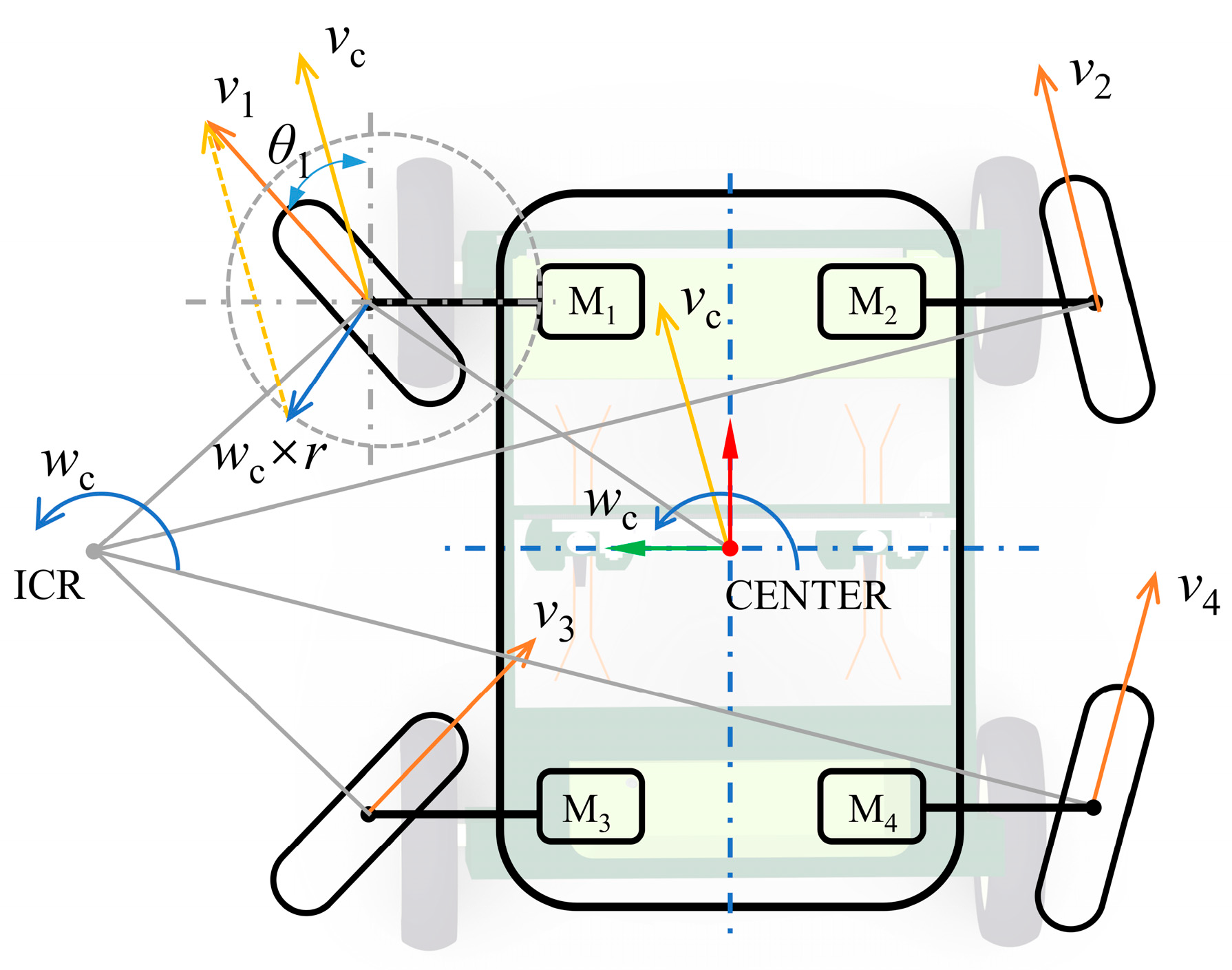
The UDV adopted in this paper is a mobile chassis with four-wheel independent steering and four-wheel independent driving, its English abbreviation is 4WIS4WID. This robot has four wheels, each equipped with two independent drive motors. It can independently control forward or backward movement, and also independently control steering. This 4WIS4WID can achieve any direction of translation or spinning motion.
At present, there have been numerous studies on the motion control and route tracking algorithms for this type of vehicle, aiming to ensure the accuracy of its route tracking [41,42,43]. The focus of this paper lies in the research of a global route planning method based on prior knowledge. This planning is completed before the actual operation of the machine, and the machine mainly serves as a platform for verifying the planned path. Therefore, the related control algorithms and route tracking algorithms are not within the scope of discussion.
As shown in Figure 16, the kinematic model of the four-wheel four-turn platform needs to establish the relationship between the rotational speeds, rotational angles of the four wheels and the geometric center velocity. In the figure, a coordinate system is established with the geometric center (CENTER) of the robot as the origin: the red arrow indicates the forward direction of the robot, which is the positive direction of the x-axis, the green arrow indicates the direction perpendicular to the x-axis to the left, which is the positive direction of the y-axis, and the z-axis is perpendicular to the paper and outward, in accordance with the right-hand rule. ICR (Instantaneous Center of Rotation) represents the instantaneous turning center.
The velocity vc of the center point can be decomposed into two component velocities along the coordinate axes, as shown by the yellow arrows in the figure, and is denoted as (vcx, vcy, wc)T. The velocity components (vcx, vcy)T are positive in the direction of the coordinate axis and negative in the opposite direction; wc represents the angular velocity of the point. The vector ri represents the vector from the center point to the contact points of each driving wheel with the ground, and vector ri can be decomposed into two component vectors (rix, riy)T along the coordinate axes. wc × ri represents the component velocity generated by the robot spinning at angular velocity wc, corresponding to the light blue arrow in the figure. The magnitude and direction of this component velocity follow the right-hand rule.
v i = v i x v i y = v i cos θ i v i sin θ i = v c x w c r i y v c y + w c r i x
in which vi represents the linear velocities (v1~v4) of each wheel of the UDV. The attitude angles θi of each driving wheel are reversibly derived from the velocity through Equation (35). Once the current speed of the vehicle is known, the speed and steering angle of each wheel can be calculated in reverse, thereby calculating the actual motion state of the vehicle and providing a basis for precise control and path tracking.

4.2.2. Rectangular Field Example

Rectangular fields are the most fundamental for maize detasseling operations. In Section 4.1, a rectangular field model was used to investigate the mechanisms of DRDM-AACO and confirm its applicability. In this section, additional rectangular fields with different sizes are analyzed to evaluate the performance of DRDM-AACO further. Furthermore, the Greedy Algorithm, the Boustrophedon Algorithm, and the Improved Boustrophedon Algorithm are applied for comparative analysis to assess the advantages of DRDM-AACO relative to other commonly used algorithms in the rectangular field problem model.
During the operation of agricultural machinery, the Boustrophedon Algorithm is frequently used to design the operational route. The traditional Boustrophedon Algorithm employs a serpentine route strategy, enabling systematic traversal of operational rows through reciprocating motion and thereby ensuring comprehensive coverage of the operational area. To better align this Boustrophedon Algorithm with the problem model presented in this paper, an improved version of the Boustrophedon Algorithm has been developed. This Improved Boustrophedon Algorithm retains the core logic of the traditional serpentine route while avoiding the traversal of aisles that lack male flower projection nodes, thus significantly reducing the total length of the operational routes.
The settings of the rectangular field model are shown in Table 7, with areas of 1 mu, 2 mu, and 3 mu, respectively. The row spacing, plant spacing of maize plants, the width of the detasseling operation of the detasseling vehicle, and the related parameters of the DRDM-AACO are the same as those in Section 4.1.
The calculation results are presented in Table 8, which displays the total lengths of the detasseling operation routes obtained using DRDM-AACO, the Greedy Algorithm, the Boustrophedon Algorithm, and the Improved Boustrophedon Algorithm. Additionally, Table 8 provides a comparison of the computational outcomes achieved by these algorithms.
Due to the substantial number of male flower nodes, it is considerably challenging to visualize the detasseling operation route. One optimization result of the DRDM-AACO is presented in Table 9, aiming to illustrate the route recording mechanism proposed.
In the “The detasseling sequence” column of Table 9, the sequence of male flower nodes in the generated detasseling operation route is recorded. For instance, the first row of data “01 02 03 04 06 07 05 29 35 30” indicates that the detasseling operation route starts from initially set male flower node 1 and successively passes through initially set male flower nodes 2, 3, 4, 6, 7, 5, 29, 35, and 30. The “The detasseling approach” column records the corresponding endpoints of the aisles to the sequence of male flower nodes. For example, the first data “S1” corresponds to male flower node 1, indicating that the detasseling operation route reaches male flower node 1 from aisle endpoint S1.
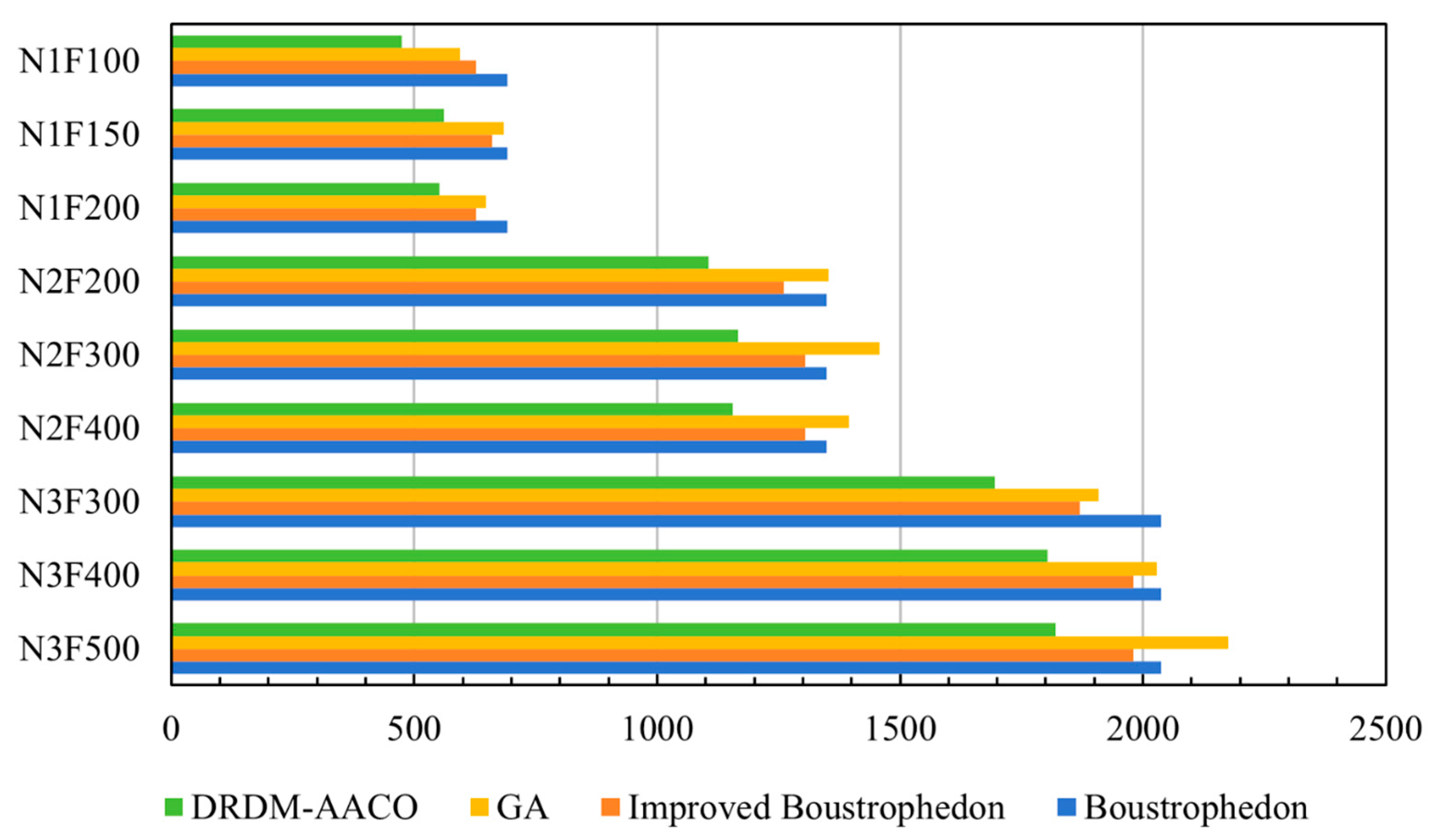
After plotting the data in Table 8, it can be clearly seen that in any of the set scenes, the total length of the route obtained by the DRDM-AACO is the shortest. Compared with the results calculated by the Greedy Algorithm, the optimization rate is 11% to 20%; compared with the results calculated by the Boustrophedon Algorithm, the optimization rate is 11% to 32%; and compared with the results calculated by the Improved Boustrophedon Algorithm, the optimization rate is 8% to 24%. The data indicates that the DRDM-AACO outperforms other commonly used algorithms, showing a significant advantage in reducing the total length of the detasseling operation route, fully demonstrating its superiority in the route planning for maize detasseling.
As shown in Figure 17, it is clear that the DRDM-AACO produces the shortest route in all scenes. Compared to the Greedy algorithm, the optimization rate is 11% to 20%. Compared to the Boustrophedon Algorithm, it is 11% to 32%. And compared to the Improved Boustrophedon Algorithm, it is 8% to 24%. These results show that the DRDM-AACO outperforms other common algorithms, significantly reducing the total detasseling operation route length and demonstrating its superiority in route planning for maize detasseling.
The data in Table 8 also shows that as the number of male flower nodes increases and the field size grows, the optimization rate of the DRDM-AACO compared to other algorithms shows a decreasing trend. For instance, in the N1 scene, as the number of male flower nodes increases, the optimization rate of the DRDM-AACO compared to the Improved Boustrophedon Algorithm drops from 25% to 12%. And this optimization rate, with the increase in field size, decreases from 25% to 9%. Although the optimization rate of the DRDM-AACO compared to other algorithms decreases in large-sized fields due to the large base value of the total route length, the actual reduction in the total route length is also significant. For example, in the N3F300 scene, the total route length optimized by the DRDM-AACO is 214 m shorter than that of the Greedy Algorithm, 342 m shorter than that of the Boustrophedon, and 175 m shorter than that of the Improved Boustrophedon. These figures are of the same order of magnitude as the total route lengths generated by each algorithm in the N1 scene.
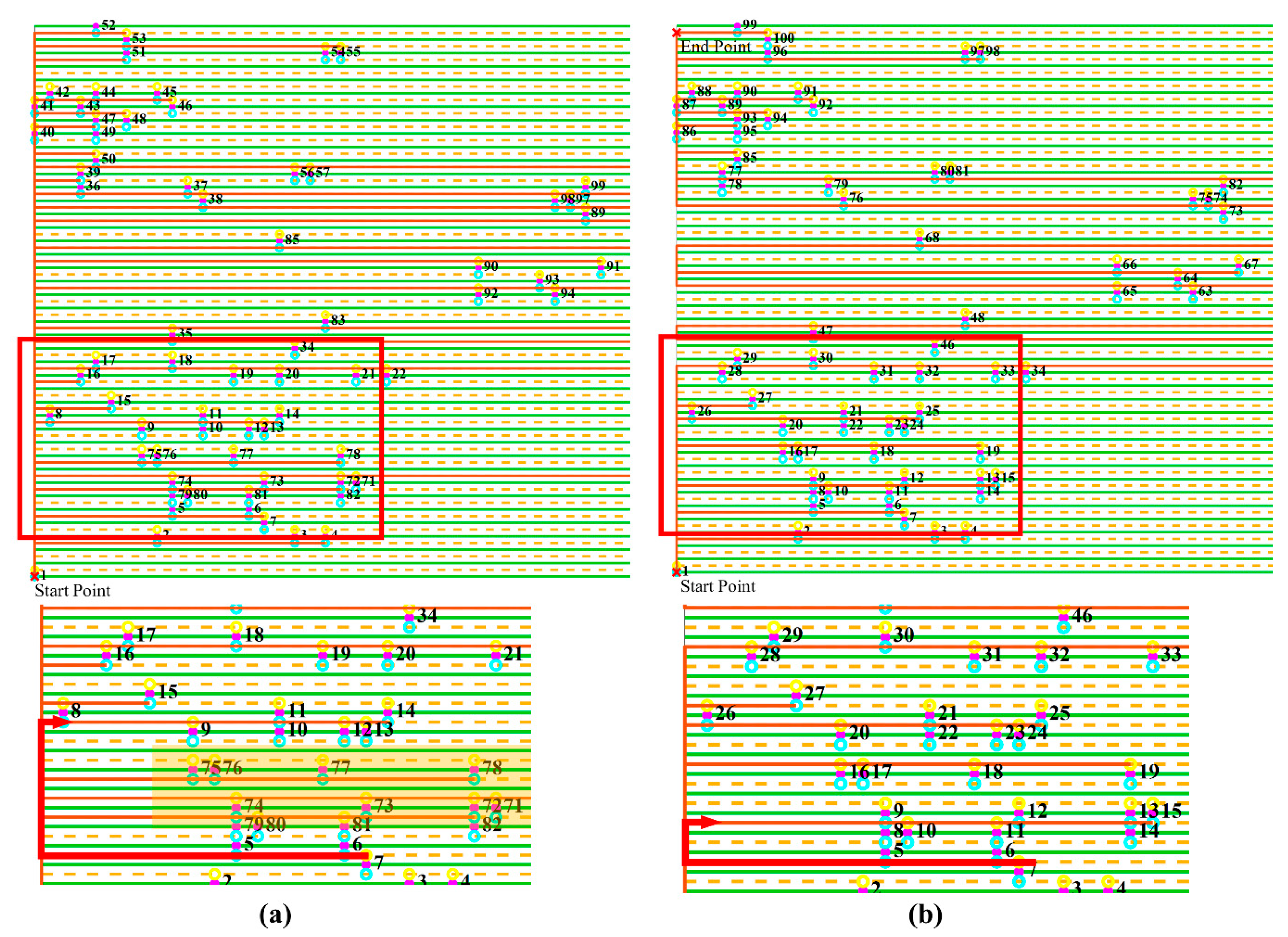
The detasseling operation route generated by the DRDM-AACO is superior to that of the Greedy Algorithm, mainly because the DRDM-AACO has the ability to globally optimize, while the Greedy Algorithm does not. The Greedy Algorithm determines the detasseling operation route through a single-step optimal selection strategy. That is when choosing the next male flower node, it prioritizes the male flower node closest to the current one. This short-sighted selection strategy ignores the global accessibility characteristics of subsequent male flower nodes. This mechanism of the Greedy Algorithm, when solving the maize detasseling operation route planning problem model in this paper, tends to generate non-continuous inter-row jumping routes, resulting in more turnback routes. For example, Figure 18a shows the detasseling operation route generated by the Greedy Algorithm in the N1F100 scene, where the male flower nodes are labeled in the order of detasseling operation. In Figure 18a, the UDV starts from the male flower node f7 and selects the nearest male flower node f8. The male flower nodes f7 and f8 are several rows apart, causing the UDV to ignore the male flower nodes between the two rows (the yellow area in Figure 18a), and these male flower nodes must be reached by generating return routes later, which increases the overall route length.
The DRDM-AACO combines the global optimization capability of ACO with a dynamic candidate set, non-uniform initial pheromone allocation, and a direction-constrained adaptive dual-mode pheromone regulation mechanism. These mechanisms prevent suboptimal routes. As shown in Figure 18b, after one optimization in the N1F100 scene, the detasseling operation route avoids selecting the nearest male flower point f26 and instead chooses f8 in the adjacent crop row, which improves the overall route efficiency.
Since the Boustrophedon Algorithm generates full coverage routes for fields of various sizes, its total route length depends only on field size, not on the number of male flower nodes. The Improved Boustrophedon Algorithm removes invalid routes, reducing the total length. In most cases, it outperforms the Greedy Algorithm. This paper focuses on why the DRDM-AACO’s results are better and does not detail the Boustrophedon. The Improved Boustrophedon Algorithm selects the nearest aisle row with male flower to ensure route continuity, but lacks global optimization and ignores actual distances between sequential male flower points. This can lead to detours when solving the maize detasseling operation route planning problem, as shown in Figure 19a,b for the N1F100 scene.

4.2.3. Actual Farmland Example

Actual fields may have polygonal boundaries. To further validate the practicality of DRDM-AACO in optimizing UDV operation paths, field comparison experiments were conducted using DRDM-AACO, Boustrophedon, Improved Boustrophedon, and Greedy Algorithm.
The experiment was conducted in a specific area under relatively stable and homogeneous soil conditions. The yaw deviation caused by field heterogeneity can be corrected by the UDV’s onboard control algorithm to ensure accurate route tracking. The experimental field environment was previously surveyed to eliminate unexpected dynamic obstacles such as pedestrians or other working vehicles during operations, thereby preventing UDV travel interruptions due to such disturbances.
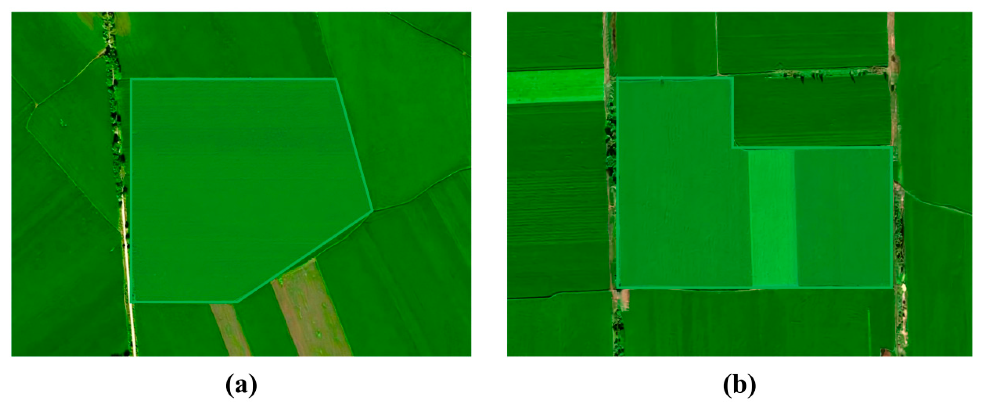
The experimental site was located in the farmland under the jurisdiction of Chajiawobao, Harbin City, Heilongjiang Province (126.65° E, 45.50° N). The actual plot boundaries were obtained from Amap. As shown in Figure 20, the selected farmland distribution had convex polygon boundaries and concave polygon boundaries.
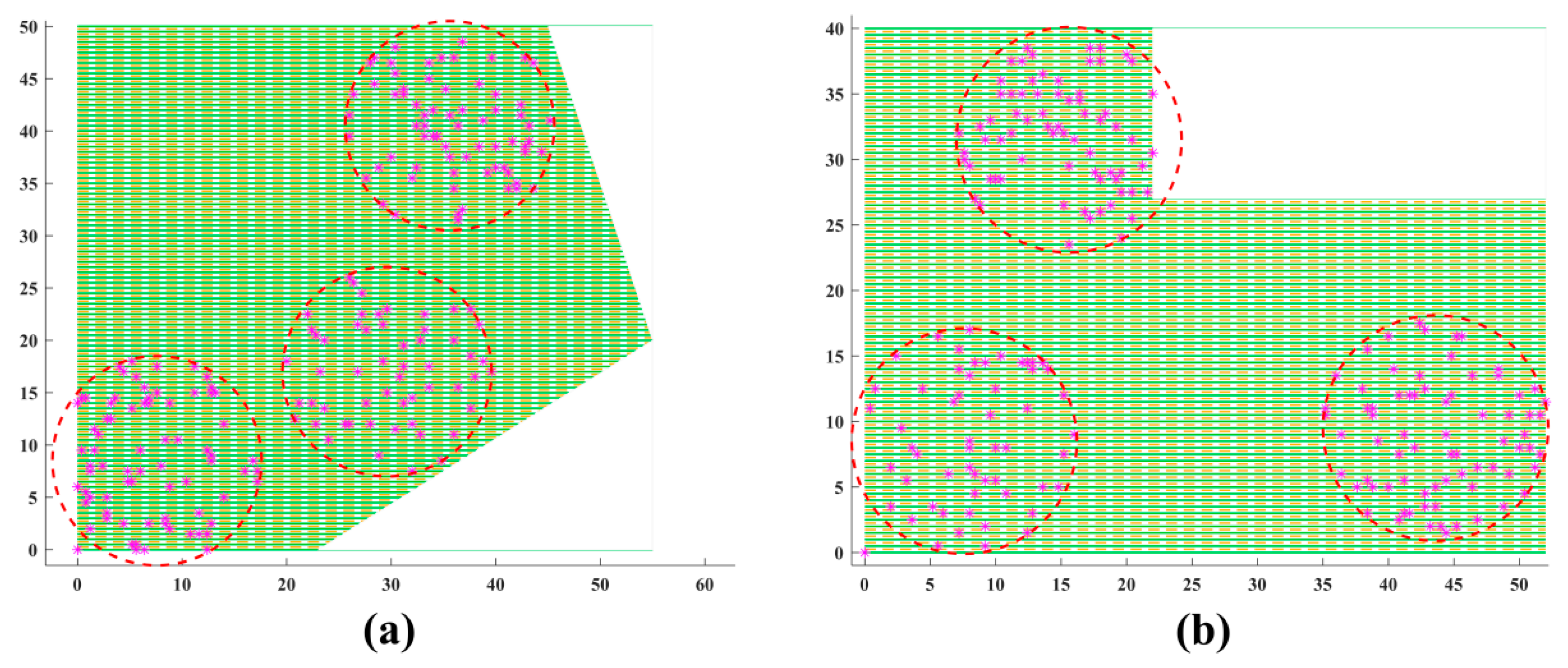
Parameters for the area of each farmland were obtained through on-site measurements, and a field model was established, as shown in Figure 21. The total number of male flowers, row spacing, planting spacing, detasseling vehicle operation width, and relevant parameter settings of the DRDM-AACO algorithm are the same as those in Section 4.2.1.
The calculated results are shown in Table 10. The table presents a comparison of detasseling route distance calculated by the DRDM-AACO, Greedy Algorithm, Boustrophedon Algorithm, and Improved Boustrophedon Algorithm, as well as their respective computational results. The average value of the DRDM-AACO results in the table is the average of 20 calculations.
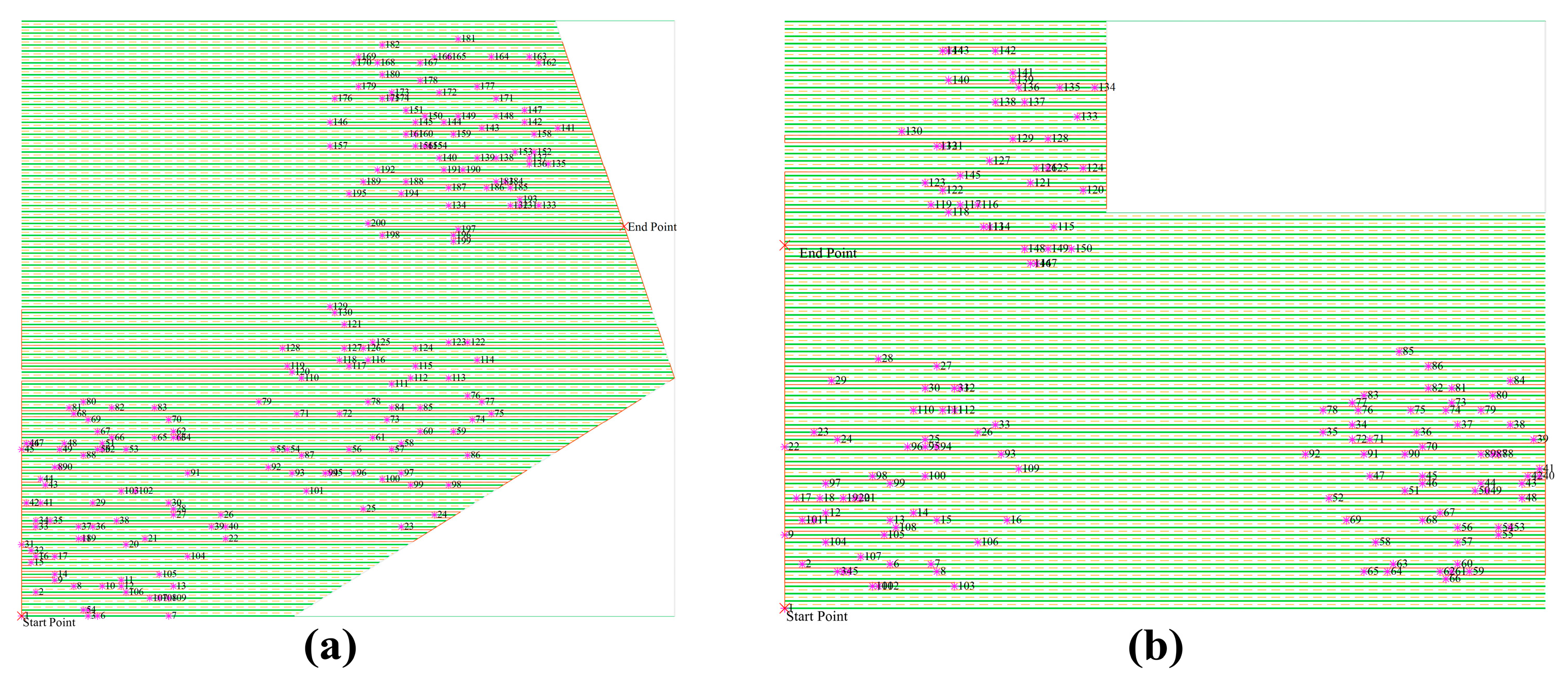
As shown in Table 10, DRDM-AACO is highly applicable to the polygonal field scenarios that exist in actual situations, and still exhibits significant performance advantages over other algorithms. This is attributed to the fact that changes in field boundaries do not interfere with the operation of the core mechanism of DRDM-AACO. As detailed in Section 2.4, alterations in field boundaries only influence the calculation method for the distance between male flower nodes. However, the DRDM-AACO optimization process directly uses these precomputed distances. Figure 22 shows the UDV operation route map for farmland 1 and farmland 2 based on the DRDM-AACO.
In the farmland 1 example, the DRDM-AACO shows an optimization rate of 14% to 23% compared to the Boustrophedon Algorithm, 4% to 7% compared to the improved Boustrophedon Algorithm, and 9% to 15% compared to the Greedy Algorithm. Results indicate that DRDM-AACO produces the shortest route, followed by the improved Boustrophedon Algorithm. The Greedy Algorithm performs poorly, with results similar to the Boustrophedon Algorithm, even in fields with 200 male flower nodes where it underperforms compared to the Boustrophedon method.
It can be seen from the results that the optimization result of DRDM-AACO is the shortest, followed by the calculation result of the improved Boustrophedon Algorithm. The greedy algorithm performs poorly, but it is better than the all-coverage improved Boustrophedon Algorithm. In the actual farmland, as the number of male flower nodes increases, the optimization rate of DRDM-AACO decreases compared to the improved Boustrophedon Algorithm, consistent with the trend in the rectangular field. This is because, within a fixed area of field, as the number of male flower nodes increases, the spatial distribution characteristics of male flower nodes tend to become less distinct. The concept of limits can be used to analyze this issue. When all plants require detasseling, the comprehensive coverage route planned through the Boustrophedon Algorithm represents the most efficient method. This further demonstrates that the DRDM-AACO is more proficient at capturing the spatial distribution characteristics of male flower nodes, consequently improving the efficiency of route planning for detasseling operations in maize seed production fields. As the number of male flower nodes increases, the runtime of DRDM-AACO will also increase. To balance calculation efficiency and result quality when dealing with a large number of male flower nodes, it is appropriate to adopt the improved Boustrophedon Algorithm.

5. Conclusions

This paper explores the route planning challenge for detasseling in maize seed production. It introduces a new algorithm: the Dual-Route and Dual-Mode Adaptive Ant Colony Optimization (DRDM-AACO), which combines multiple mechanisms for hybrid spatial constrained features.
First, a mathematical model was established to optimize detasseling route planning in maize seed production fields. In this model, the set of male flower nodes and the set of crop rows served as inputs, while the detasseling sequence and the approach to each male flower node were defined as outputs. The objective function was formulated to minimize the total length of the detasseling routes. The model proposed a method to establish the projection nodes of male flower spots on different aisles to adapt to the characteristics of the UDV double-row operation width. And based on the projection nodes, a multi-dimensional distance matrix was constructed as the input of DRDM-AACO. Second, the ant colony algorithm was improved through four synergistic mechanisms: (1) Dual-route preference mechanism, (2) Dynamic candidate set mechanism, (3) Non-uniform initial pheromone allocation mechanism, (4) Direction-constrained adaptive dual-mode pheromone regulation mechanism. The proposed algorithm was compared with five algorithms, including ACO and its variants, through example experiments.
The experiment shows that the dual-route preference mechanism increases route diversity and enhances the global optimization ability of the algorithm by improving the heuristic information of the main and auxiliary routes. The non-uniform initial pheromone allocation mechanism guides the UDV to prioritize exploring potential optimal regions by enhancing the pheromone concentration of intra-row routes while weakening that of inter-row routes in the initial environment. The direction-constrained adaptive dual-mode pheromone regulation mechanism addresses the issue of generating turnback routes within a single aisle through the integration of a local pheromone penalty mechanism and an adaptive global evaporation strategy. Through the synergistic operation of four mechanisms, the performance of DRDM-AACO has been significantly enhanced, resulting in optimization results that exhibit a maximum improvement rate of up to 6% compared to ACO. Finally, DRDM-AACO was also applied to conduct example experiments on fields of different sizes and actual farmland. The outcomes were compared against those of three widely adopted algorithms: the Greedy Algorithm, the Boustrophedon Algorithm, and the Improved Boustrophedon Algorithm. Experiments show that DRDM-AACO demonstrates superior performance in various field examples of different sizes and boundary shapes. The optimization results achieved by DRDM-AACO are 11% to 20% shorter than those obtained using the Greedy Algorithm, 11% to 32% shorter than those of the Boustrophedon Algorithm, and 5% to 25% shorter than those of the Improved Boustrophedon Algorithm.
Research demonstrates that the DRDM-AACO proposed in this paper is capable of efficiently generating shorter detasseling operation routes, thereby enhancing the efficiency of detasseling operations in maize seed production fields. Additionally, it contributes to further elevating the automation and intelligence levels of unmanned detasseling vehicles.
Moreover, with minor adjustments, the DRDM-AACO can be effectively adapted for application in agricultural machinery of diverse working widths. Consequently, this study proposes a novel methodology for addressing heterogeneous Traveling Salesman Problem (TSP) models, especially route planning challenges in agricultural production.
In the current study, it is essential to explicitly acknowledge several limitations. The proposed DRDM-AACO algorithm mainly focuses on global route planning for male flower nodes at known locations and is validated based on the homogeneous characteristics of maize detasseling fields. It does not investigate real-time dynamic path planning algorithms for UDV operation in the field. The homogeneous environment mentioned in this study limits the impact of issues such as UDV slippage, drift, and increased travel distance caused by factors like soil conditions on the global route planning. Furthermore, this study does not address the situation requiring real-time path planning when obstacles of varying sizes suddenly appear outside the predefined detection range. This paper focuses only on global route planning based on prior knowledge. Real-time obstacle avoidance and course correction are part of real-time path planning, representing another worthy research direction. To further enhance route planning accuracy, addressing the coordination between global route planning and real-time path planning is essential.
The research and application of DRDM-AACO are still in early stages and have limitations that require further exploration. Research can be further explored in the following directions: 1) Cross-field operation route optimization. (1) Cross-field operation route optimization. The multi-field coupling model is constructed to systematically address connection route generation and operation sequence optimization. (2) Multi-machine collaborative scheduling strategy. Using the vehicle routing problem (VRP) framework, route optimization for multiple UDVs operating in large field areas is developed. (3) Develop a hierarchical decision-making framework that combines the global optimization path with the real-time perceived dynamic environmental information. This framework will enable the UDV to efficiently adjust its path upon encountering new information such as obstacles and slippage, thereby ensuring the integrity and efficiency of the operation.
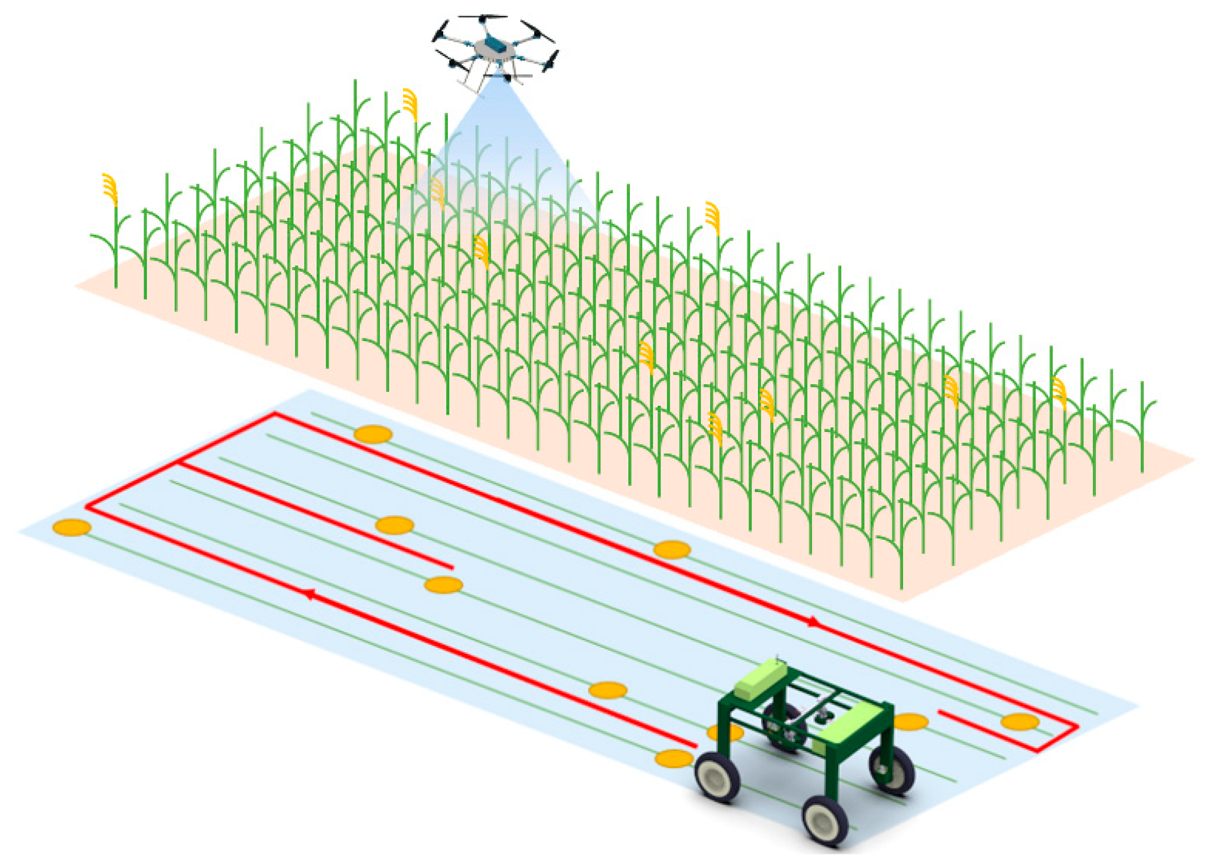
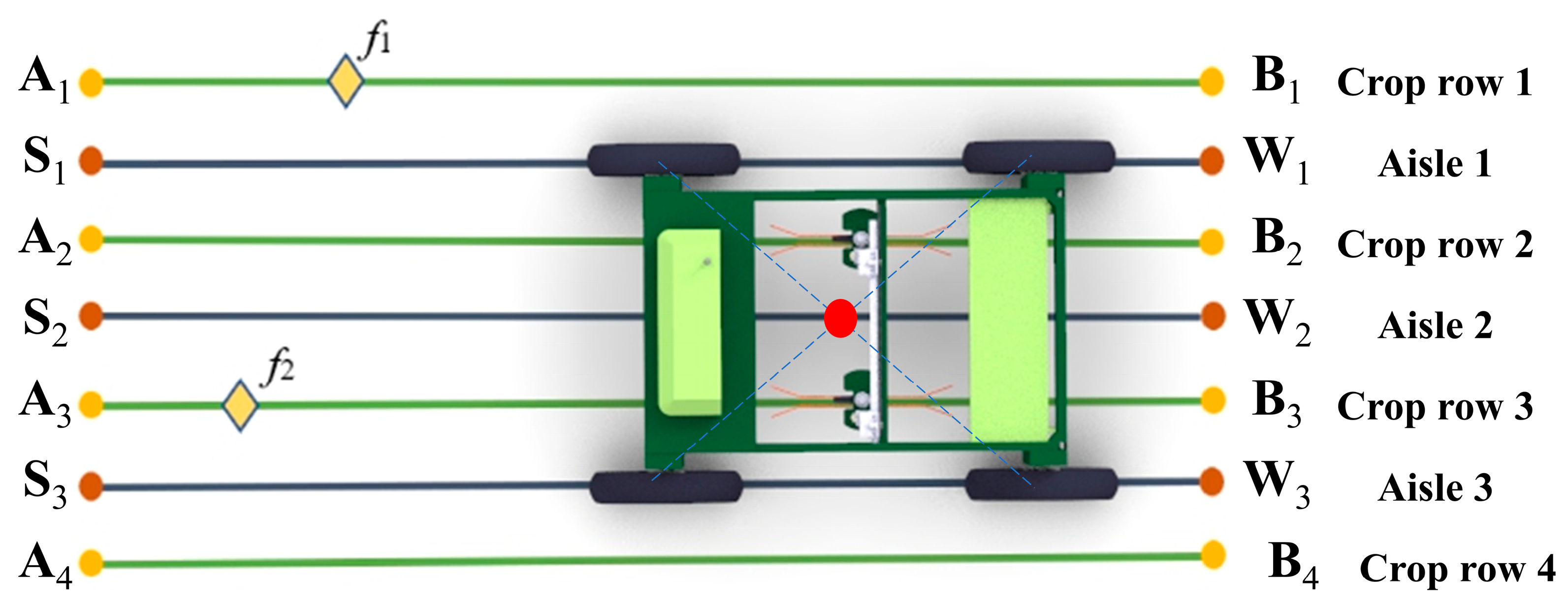
Author Contributions

Conceptualization, Y.W.; methodology, Y.W. and Y.Y.; software, Y.Y.; validation, Y.W. and Y.Y.; formal analysis, Y.W.; investigation, Y.Z.; data curation, Y.Z.; writing—original draft preparation, Y.Y.; writing—review and editing, L.L.; visualization, L.G.; supervision, L.L.; project administration, L.L.; funding acquisition, Y.W. All authors have read and agreed to the published version of the manuscript.

Funding

This research was funded by National Key Research and Development Program of China, grant number 2021YFD2000405-2. The APC was funded by Northeast Agricultural University.

Data Availability Statement

The original contributions presented in this study are included in this article. Further inquiries can be directed to the corresponding author(s).

Conflicts of Interest

The authors declare no conflicts of interest.

Abbreviations

The following abbreviations are used in this manuscript:
UDVUnmanned maize detasseling vehicle
DRDM-AACODual-Route and Dual-Mode Adaptive Ant Colony Optimization
ACOAnt Colony Optimization
TSPTraveling Salesman Problem
UAVUnmanned Aerial Vehicle
OPTOptimization

References

  1. Sun, Q.; Gu, X.; Chen, L.; Xu, X.; Wei, Z.; Pan, Y.; Gao, Y. Monitoring Maize Canopy Chlorophyll Density under Lodging Stress Based on UAV Hyperspectral Imagery. Comput. Electron. Agric. 2022, 193, 106671. [Google Scholar] [CrossRef]
  2. Tian, J.; Wang, C.; Xia, J.; Wu, L.; Xu, G.; Wu, W.; Li, D.; Qin, W.; Han, X.; Chen, Q.; et al. Teosinte Ligule Allele Narrows Plant Architecture and Enhances High-Density Maize Yields. Science 2019, 365, 658–664. [Google Scholar] [CrossRef] [PubMed]
  3. Chen, S.; Liu, W.; Morel, J.; Parsons, D.; Du, T. Improving Yield, Quality, and Environmental Co-Benefits through Optimized Irrigation and Nitrogen Management of Hybrid Maize in Northwest China. Agric. Water Manag. 2023, 290, 108577. [Google Scholar] [CrossRef]
  4. Li, X.; Zhang, S.; Shao, P. Impact of Recent Breeding History on the Competitiveness of Chinese Maize Hybrids. Eng. Appl. Artif. Intell. 2024, 131, 107816. [Google Scholar] [CrossRef]
  5. Pan, X.; Zhang, H.; Yu, S.; Deng, H.; Chen, X.; Zhou, C.; Li, F. Strategies for the Management of Water and Nitrogen Interaction in Seed Maize Production; A Case Study from China Hexi Corridor Oasis Agricultural Area. Agric. Water Manag. 2024, 292, 108685. [Google Scholar] [CrossRef]
  6. Shi, R.; Wang, J.; Tong, L.; Du, T.; Shukla, M.K.; Jiang, X.; Li, D.; Qin, Y.; He, L.; Bai, X.; et al. Optimizing Planting Density and Irrigation Depth of Hybrid Maize Seed Production under Limited Water Availability. Agric. Water Manag. 2022, 271, 107759. [Google Scholar] [CrossRef]
  7. Song, C.; Zhang, F.; Xie, J.; Yang, C.; Li, J.; Zhang, J. Development and Evaluation of a Novel Maize Detasseling Device. Comput. Electron. Agric. 2024, 221, 108944. [Google Scholar] [CrossRef]
  8. Du, J.; Li, J.; Fan, J.; Gu, S.; Guo, X.; Zhao, C. Detection and Identification of Tassel States at Different Maize Tasseling Stages Using UAV Imagery and Deep Learning. Plant Phenomics 2024, 6, 0188. [Google Scholar] [CrossRef]
  9. Jia, Y.; Fu, K.; Lan, H.; Wang, X.; Su, Z. Maize Tassel Detection with CA-YOLO for UAV Images in Complex Field Environments. Comput. Electron. Agric. 2024, 217, 108562. [Google Scholar] [CrossRef]
  10. Yang, J.; Zhang, R.; Ding, C.; Chen, L.; Xie, Y.; Ou, H. YOLO-Detassel: Efficient Object Detection for Omitted Pre-Tassel in Detasseling Operation for Maize Seed Production. Comput. Electron. Agric. 2025, 231, 109951. [Google Scholar] [CrossRef]
  11. Toaza, B.; Esztergar-Kiss, D. A Review of Metaheuristic Algorithms for Solving TSP-Based Scheduling Optimization Problems. Appl. Soft Comput. 2023, 148, 110908. [Google Scholar] [CrossRef]
  12. Utamima, A.; Djunaidy, A. Agricultural Routing Planning: A Narrative Review of Literature. Procedia Comput. Sci. 2022, 197, 693–700. [Google Scholar] [CrossRef]
  13. Sarkar, R.; Barman, D.; Chowdhury, N. Domain Knowledge Based Genetic Algorithms for Mobile Robot Path Planning Having Single and Multiple Targets. J. King Saud Univ.-Comput. Inf. Sci. 2022, 34, 4269–4283. [Google Scholar] [CrossRef]
  14. Liu, X.; Li, G.; Yang, H.; Zhang, N.; Wang, L.; Shao, P. Agricultural UAV Trajectory Planning by Incorporating Multi-Mechanism Improved Grey Wolf Optimization Algorithm. Expert Syst. Appl. 2023, 233, 120946. [Google Scholar] [CrossRef]
  15. Pehlivanoglu, Y.V.; Pehlivanoglu, P. An Enhanced Genetic Algorithm for Path Planning of Autonomous UAV in Target Coverage Problems. Appl. Soft Comput. 2021, 112, 107796. [Google Scholar] [CrossRef]
  16. Guo, H.; Mao, Z.; Ding, W.; Liu, P. Optimal Search Path Planning for Unmanned Surface Vehicle Based on an Improved Genetic Algorithm. Comput. Electr. Eng. 2019, 79, 106467. [Google Scholar] [CrossRef]
  17. Yakoubi, M.A.; Laskri, M.T. The Path Planning of Cleaner Robot for Coverage Region Using Genetic Algorithms. J. Innov. Digit. Ecosyst. 2016, 3, 37–43. [Google Scholar] [CrossRef]
  18. Lamini, C.; Benhlima, S.; Elbekri, A. Genetic Algorithm Based Approach for Autonomous Mobile Robot Path Planning. Procedia Comput. Sci. 2018, 127, 180–189. [Google Scholar] [CrossRef]
  19. Song, B.; Wang, Z.; Zou, L. An Improved PSO Algorithm for Smooth Path Planning of Mobile Robots Using Continuous High-Degree Bezier Curve. Appl. Soft Comput. 2021, 100, 106960. [Google Scholar] [CrossRef]
  20. Guo, X.; Ji, M.; Zhao, Z.; Wen, D.; Zhang, W. Global Path Planning and Multi-Objective Path Control for Unmanned Surface Vehicle Based on Modified Particle Swarm Optimization (PSO) Algorithm. Ocean Eng. 2020, 216, 107693. [Google Scholar] [CrossRef]
  21. Ajeil, F.H.; Ibraheem, I.K.; Sahib, M.A.; Humaidi, A.J. Multi-Objective Path Planning of an Autonomous Mobile Robot Using Hybrid PSO-MFB Optimization Algorithm. Appl. Soft Comput. 2020, 89, 106076. [Google Scholar] [CrossRef]
  22. Liu, Y.; Zhang, X.; Zhang, Y.; Guan, X. Collision Free 4D Path Planning for Multiple UAVs Based on Spatial Refined Voting Mechanism and PSO Approach. Chin. J. Aeronaut. 2019, 32, 1504–1519. [Google Scholar] [CrossRef]
  23. Girija, S.; Joshi, A. Fast Hybrid PSO-APF Algorithm for Path Planning in Obstacle Rich Environment. IFAC-Pap. 2019, 52, 25–30. [Google Scholar] [CrossRef]
  24. Oliveira, R.; Ljungqvist, O.; Lima, P.F.; Wahlberg, B. Optimization-Based On-Road Path Planning for Articulated Vehicles. IFAC-Pap. 2020, 53, 15572–15579. [Google Scholar] [CrossRef]
  25. Das, P.K.; Jena, P.K. Multi-Robot Path Planning Using Improved Particle Swarm Optimization Algorithm through Novel Evolutionary Operators. Appl. Soft Comput. 2020, 92, 106312. [Google Scholar] [CrossRef]
  26. Borish, M.; Wade, C. A GPU-Based Approach for Path Planning Optimization via Travel Length Reduction. Procedia Manuf. 2021, 53, 310–317. [Google Scholar] [CrossRef]
  27. Wu, L.; Huang, X.; Cui, J.; Liu, C.; Xiao, W. Modified Adaptive Ant Colony Optimization Algorithm and Its Application for Solving Path Planning of Mobile Robot. Expert Syst. Appl. 2023, 215, 119410. [Google Scholar] [CrossRef]
  28. Cui, J.; Wu, L.; Huang, X.; Xu, D.; Liu, C.; Xiao, W. Multi-Strategy Adaptable Ant Colony Optimization Algorithm and Its Application in Robot Path Planning. Knowl.-Based Syst. 2024, 288, 111459. [Google Scholar] [CrossRef]
  29. Liu, C.; Wu, L.; Huang, X.; Xiao, W. Improved Dynamic Adaptive Ant Colony Optimization Algorithm to Solve Pipe Routing Design. Knowl.-Based Syst. 2022, 237, 107846. [Google Scholar] [CrossRef]
  30. Miao, C.; Chen, G.; Yan, C.; Wu, Y. Path Planning Optimization of Indoor Mobile Robot Based on Adaptive Ant Colony Algorithm. Comput. Ind. Eng. 2021, 156, 107230. [Google Scholar] [CrossRef]
  31. Wang, Z.; Zhu, X.; Han, Q. Mobile Robot Path Planning Based on Parameter Optimization Ant Colony Algorithm. Procedia Eng. 2011, 15, 2738–2741. [Google Scholar] [CrossRef]
  32. Zhang, Y.-Q.; Wang, J.-H.; Wang, Y.; Jia, Z.-C.; Sun, Q.; Pei, Q.-Y.; Wu, D. Intelligent Planning of Fire Evacuation Routes in Buildings Based on Improved Adaptive Ant Colony Algorithm. Comput. Ind. Eng. 2024, 194, 110335. [Google Scholar] [CrossRef]
  33. Li, K.; Ge, F.; Han, Y.; Wang, Y.; Xu, W. Path Planning of Multiple UAVs with Online Changing Tasks by an ORPFOA Algorithm. Eng. Appl. Artif. Intell. 2020, 94, 103807. [Google Scholar] [CrossRef]
  34. Ray, S.S.; Misra, S. Genetic Algorithm for Assigning Weights to Gene Expressions Using Functional Annotations. Comput. Biol. Med. 2019, 104, 149–162. [Google Scholar] [CrossRef]
  35. Lesch, V.; König, M.; Kounev, S.; Stein, A.; Krupitzer, C. Tackling the Rich Vehicle Routing Problem with Nature-Inspired Algorithms. Appl. Intell. 2022, 52, 9476–9500. [Google Scholar] [CrossRef]
  36. Agrawal, A.; Ghune, N.; Prakash, S.; Ramteke, M. Evolutionary Algorithm Hybridized with Local Search and Intelligent Seeding for Solving Multi-Objective Euclidian TSP. Expert Syst. Appl. 2021, 181, 115192. [Google Scholar] [CrossRef]
  37. Yılmaz, C.; Cengiz, E.; Kahraman, H.T. A New Evolutionary Optimization Algorithm with Hybrid Guidance Mechanism for Truck-Multi Drone Delivery System. Expert Syst. Appl. 2024, 245, 123115. [Google Scholar] [CrossRef]
  38. Liang, C.; Pan, K.; Zhao, M.; Lu, M. Multi-Node Path Planning of Electric Tractor Based on Improved Whale Optimization Algorithm and Ant Colony Algorithm. Agriculture 2023, 13, 586. [Google Scholar] [CrossRef]
  39. Cerdeira-Pena, A.; Carpente, L.; Amiama, C. Optimised Forage Harvester Routes as Solutions to a Traveling Salesman Problem with Clusters and Time Windows. Biosyst. Eng. 2017, 164, 110–123. [Google Scholar] [CrossRef]
  40. Cariou, C.; Gobor, Z. Trajectory Planning for Robotic Maintenance of Pasture Based on Approximation Algorithms. Biosyst. Eng. 2018, 174, 219–230. [Google Scholar] [CrossRef]
  41. Sánchez, J.A.S.; López-González, E.; Magid, E.; Martínez-García, E.A. Double Spiraliform Path Planning and Tracking for Agricultural Mobile Robotics: A Modeling and Simulation Study. Comput. Electron. Agric. 2025, 237, 110715. [Google Scholar] [CrossRef]
  42. Zhou, J.; Wen, J.; Yao, L.; Yang, Z.; Xu, L.; Yao, L. Agricultural Machinery Path Tracking with Varying Curvatures Based on an Improved Pure-Pursuit Method. Agriculture 2025, 15, 266. [Google Scholar] [CrossRef]
  43. Amertet, S.; Gebresenbet, G.; Alwan, H.M. Optimizing the Performance of a Wheeled Mobile Robots for Use in Agriculture Using a Linear-Quadratic Regulator. Robot. Auton. Syst. 2024, 174, 104642. [Google Scholar] [CrossRef]
Figure 1. UDV operates with data collected by UAV.
Agriculture 15 02062 g001
Figure 2. The input information of the model.
Agriculture 15 02062 g002
Figure 3. Four different routes from U1.
Agriculture 15 02062 g003
Figure 4. Four different routes from V1.
Agriculture 15 02062 g004
Figure 5. The special situation in the field. (a) The projection nodes are located on the same aisle; (b) Male flowers are on the same crop row.
Agriculture 15 02062 g005
Figure 6. Specific routes represented by the output information in Table 1.
Agriculture 15 02062 g006
Figure 7. Model of the field with polygonal boundary. (a) Convex polygonal field; (b) Concave polygonal field.
Agriculture 15 02062 g007
Figure 8. Schematic diagram of the dynamic candidate set in maize detasseling operations.
Agriculture 15 02062 g008
Figure 9. Schematic diagram of the differences between the traditional TSP and the actual field work.
Agriculture 15 02062 g009
Figure 10. The flowchart of the DRDM-AACO.
Agriculture 15 02062 g010
Figure 11. A map of the distribution of male flowers generated with 100 male flowers per mu.
Agriculture 15 02062 g011
Figure 12. (a) Optimal routes generated by ACO; (b) Optimal routes generated by ACO-1.
Agriculture 15 02062 g012
Figure 13. The box plot between different φ0 values and distances after 20 independent calculations.
Agriculture 15 02062 g013
Figure 14. (a) Optimal routes generated by ACO-3; (b) Optimal routes generated by DRDM-AACO.
Agriculture 15 02062 g014
Figure 15. Optimal routes generated by IDAACO. (a) Partial Enlarged View of Farmland Route 1; (b) Partial Enlarged View of Farmland Route 2.
Agriculture 15 02062 g015
Figure 16. The kinematic model of the four-wheel drive and four-wheel steering chassis of UDV.
Agriculture 15 02062 g016
Figure 17. Bar chart of total route lengths calculated by various algorithms in rectangular fields.
Agriculture 15 02062 g017
Figure 18. (a) Optimal routes generated by the Greedy Algorithm; (b) Optimal routes generated by DRDM-AACO.
Agriculture 15 02062 g018
Figure 19. (a) Optimal routes generated by Improved Boustrophedon C; (b) Optimal routes generated by DRDM-AACO.
Agriculture 15 02062 g019
Figure 20. Actual farmland shapes. (a) Farmland 1 has convex polygonal boundary features; (b) Farmland 2 has concave polygonal boundary features.
Agriculture 15 02062 g020
Figure 21. Distribution map of male flowers in the actual farmland model. (a) Farmland model 1 has convex polygonal boundary features; (b) Farmland model 2 has concave polygonal boundary features.
Agriculture 15 02062 g021
Figure 22. Route maps for UDV operation planning based on DRDM-AACO. (a) Route map for farmland 1. (b) Route map for farmland 2.
Agriculture 15 02062 g022
Table 1. Examples of output information.
R1zR2z
f4w3
f30
f1s1
f20
Table 2. DRDM-AACO pseudocode.
DRDM-AACO Pseudocode
1. Input male flower endpoint coordinates, crop row endpoint coordinates
2. Initialize algorithm information, including: t, T, M, α, β, ρ, Q, τ, λ, ζ, γ, η
3. Determine and generate the main and auxiliary distance matrices
    D u   main , D u   aux , D v   main , D v   aux
4. Establish the initial non-uniform pheromone matrices by
      τ ij ( 0 ) = τ 0 · e - γ · r i - r j · ( 1 + η · δ same ( i , j ) ) · 1 1 + d i j / d max
5. Establish the pheromone volatility factor matrix [ρ(t)]N×N and the results recording matrices R 1 m t and     R 2 m t
6. While t = 1 < T do
7.  For m = 1 to M do
8.    Put all ants into the starting node to look for the route
9.    For j = 1 to N (N is the number of allowed male flowers)
10.      Generate male flower taboos, approach taboos
11.      Determine the position of the last male flower fi on the taboo table
12.      Construct the dynamic candidate set of this male flower O i   m
13.      Computes four select probabilities
14.      Put the four probabilities together
       P ij   m = τ ij   main t α · η ij   main β + τ ij   aux t α · η ij   aux β s O i m τ is   main t α · η is   main β + τ is   main t α · η is   aux β
15.      Roulette method selects one of the male flowers fj
16.      Determine whether to pass through Uj or Vj
17.      Record the position of the j-th removed male flower
18.    End For
19.    Record the distance l m t traveled by the m-th UDV
20.    Record invalid intra-row turnback routes between two nodes
21.  End For
22.  For m = 1 to M do
23.    If dij is intra-row turnback routes between two nodes
24.         Δ τ ij m t   =   Q / l m t - ζ   · Q / d ij  
25.    End If
26.  End For
27.  If dij is intra-row turnback route
28.     ρ ( t ) ρ 0 + λ · N turn / N total
29.  Else
30.     ρ ( t ) ρ 0
31.  End If
32.  Update pheromone by τ ij ( t + 1 )   =   [ 1 - ρ ( t ) ] · τ ij ( t ) + m = 1 M Δ τ ij m ( t )
33.  Record the approach to reach the z-th male flower
34.  Recording Route Information
35. End While
36. Visual drawing
37. Output optimal route
Table 3. Abbreviation for the variants of ACO, DRDM-AACO, IDAACO.
AbbreviationVariants of ACO
ACOTraditional ACO
ACO-1ACO with improvement proposed in Section 3.1 (Dual route preference)
ACO-2ACO with improvements proposed in Section 3.1 and Section 3.2 (Dual route preference, Dynamic candidate set)
ACO-3ACO with improvements proposed in Section 3.1, Section 3.2 and Section 3.3 (Dual route preference, Dynamic candidate set, Non-uniform initial pheromone allocation)
DRDM-AACOACO with all improvements proposed in Section 3.1, Section 3.2, Section 3.3 and Section 3.4 (Dual route preference, Dynamic candidate set, Non-uniform initial pheromone allocation, Direction-Constrained Adaptive Dual-model Pheromone Regulation)
IDAACOACO with all improvements proposed by Liu et al. [29]. (adaptive pseudorandom transfer strategy, improved local pheromone updating mechanism, and improved global pheromone updating mechanism)
Table 4. Parameters setting for the variants of ACO.
ParametersMTαβρQλζφ0γη
Value1503000.580.23000.350.40.250.850.6
Table 5. Experimental results of five algorithms.
Male Flowers
Number
Performance IndexACOACO-1ACO-2ACO-3DRDM-AACOIDAACO
100Average distance504.47493.35494.45480.29465.77488.25
Best distance496.75491.65478.95479.35462.85478.95
Average runtime23.2935.2322.2426.9128.9138.95
150Average distance595.80584.13583.60570.33562.37587.99
Best distance587.85582.25578.85568.15558.95581.35
Average runtime69.25117.1959.9062.0664.02109.20
200Average distance581.20563.60561.47563.37545.05576.93
Best distance576.05559.05558.45558.05541.45573.65
Average runtime138.81244.45125.63136.38114.77262.31
Table 6. Results of distance and runtime corresponding to different φ0 values.
Index0.10.150.20.250.30.350.40.450.5
Distance median/m588.15577.35568.15568.35564.60561.25566.50565.60566.30
Distance mean/m587.00576.40568.85567.37564.77561.07565.37564.52566.17
Distance OPTrate/%−3.37%−1.50%−0.18%0.09%0.54%1.19%0.44%0.59%0.30%
Runtime mean/s47.8255.1156.0259.3664.3469.1373.3477.1283.08
Runtime OPTrate/%59.50%53.32%52.56%49.73%45.51%41.45%37.89%34.69%29.64%
Table 7. Information settings of the rectangular field model.
Field NumberArea/m2Length/mWidth/mCrop RowsParent RowsDistribution Circles/m
N16563220.542355
N213224429.560507
N3197355.635.572608.6
Table 8. Optimization results for rectangular fields with varying sizes and numbers of male flowers.
Field
Number
Male Flowers NumberDRDM-AACOGreedy AlgorithmBoustrophedonImproved Boustrophedon
Distance/mDistance/mOPT Rate/%Distance/mOPT Rate/%Distance/mOPT Rate/%
100100474.08594.2520.22692.2531.52628.2524.54
150561.95685.0517.97692.2518.82660.2514.89
200552.65647.5514.66692.2520.17628.2512.03
1502001106.381352.9518.221349.2518.001261.2512.28
3001166.081457.3519.991349.2513.581305.2510.66
4001156.591394.9517.091349.2514.281305.2511.39
2003001694.651908.5511.212036.8516.801870.059.38
4001802.922028.6511.132036.8511.481981.259.00
5001821.012176.2516.322036.8510.601981.258.09
Table 9. Optimal route for rectangular field.
The Detasseling SequenceThe Detasseling Approach
01020304060705293530S1S300S500S1300
313844453940414246470S15S160000000
4348343733363222212800W130000W1100
271614111513100908120W700000000
17181920232425265549S9000S11000S180
505152535654576063650000000W19W220
62646177817882837984000S30000000
808586909391949295870S31S33S35S3600000
88899697981009968697200S3900S410S260W28
7176707574736667585900000 00S200
Table 10. Optimization results for actual farmland with varying numbers of male flowers.
Field
Number
Male Flowers NumberDRDM-AACOBoustrophedonImproved
Boustrophedon
Greedy Algorithm
Average/mDistance/mOPT Rate/%Distance/mOPT Rate/%Distance/mOPT Rate/%
convex polygon2001787.08 2309.4322.621887.93 5.34 2056.26 13.09
2501843.72 20.171983.10 7.03 2176.74 15.30
3001981.87 14.182083.99 4.90 2168.51 8.61
concave polygon1501132.63 1699.5033.351320.25 14.21 1228.75 7.82
2001255.12 26.151372.75 8.57 1564.35 19.77
2501358.25 20.071446.75 6.12 1607.85 15.52
Disclaimer/Publisher’s Note: The statements, opinions and data contained in all publications are solely those of the individual author(s) and contributor(s) and not of MDPI and/or the editor(s). MDPI and/or the editor(s) disclaim responsibility for any injury to people or property resulting from any ideas, methods, instructions or products referred to in the content.