Maize Leaf Area Index Estimation Based on Machine Learning Algorithm and Computer Vision

Abstract

Precise estimation of the leaf area index (LAI) is vital in efficient maize growth monitoring and precision farming. Traditional LAI measurement methods are often destructive and labor-intensive, while techniques relying solely on spectral data suffer from limitations such as spectral saturation. To overcome these difficulties, the study integrated computer vision techniques with UAV-based remote sensing data to establish a rapid and non-invasive method for estimating the LAI in maize. Multispectral imagery of maize was acquired via UAV platforms across various phenological stages, and vegetation features were derived based on the Excess Green (ExG) Index and the Hue–Saturation–Value (HSV) color space. LAI standardization was performed through edge detection and the cumulative distribution function. The proposed LAI estimation model, named VisLAI, based solely on visible light imagery, demonstrated high accuracy, with R² values of 0.84, 0.75, and 0.50, and RMSE values of 0.24, 0.35, and 0.44 across the big trumpet, tasseling–silking, and grain filling stages, respectively. When HSV-based optimization was applied, VisLAI achieved even better performance, with R² values of 0.92, 0.90, and 0.85, and RMSE values of 0.19, 0.23, and 0.22 at the respective stages. The estimation results were validated against ground-truth data collected using the LAI-2200C plant canopy analyzer and compared with six machine learning algorithms, including Gradient Boosting (GB), Random Forest (RF), Ridge Regression (RR), Support Vector Regression (SVR), and Linear Regression (LR). Among these, GB achieved the best performance, with R² values of 0.88, 0.88, and 0.65, and RMSE values of 0.22, 0.25, and 0.34. However, VisLAI consistently outperformed all machine learning models, especially during the grain filling stage, demonstrating superior robustness and accuracy. The VisLAI model proposed in this study effectively utilizes UAV-captured visible light imagery and computer vision techniques to achieve accurate, efficient, and non-destructive estimation of maize LAI. It outperforms traditional and machine learning-based approaches and provides a reliable solution for real-world maize growth monitoring and agricultural decision-making.

1. Introduction

The leaf area index (LAI) is an essential agronomic indicator, significantly influencing maize development and its photosynthetic efficiency. It is essential for evaluating maize development, photosynthetic efficiency, and ecological functions. The magnitude of the LAI directly affects the efficiency of photosynthesis, influencing maize growth rates, yield, and resilience to environmental stresses. As a fundamental vegetation structural parameter, the LAI is extensively used in the fields of ecology, agriculture, and climate change research. It is a unitless metric used to express the total single-sided leaf surface area per unit ground area and is widely used as an important parameter in ecological and climate models. The LAI serves as a key indicator for maize variety improvement, agricultural management, ecological monitoring, and decision-making processes in agriculture. Therefore, timely and precise LAI estimation plays a crucial role in monitoring maize development, predicting yield, and guiding field management [1].

Traditional approaches to estimating the LAI are generally categorized into direct and indirect approaches. Direct measurements require destructive sampling to obtain the maize’s leaf area. Although this approach provides high accuracy, its applicability for large-scale field monitoring is constrained by the inherently destructive nature of the sampling process and the substantial costs associated with it [2]. In contrast, the indirect measurement method determines the LAI using optical instruments (such as the LAI-2200C or fisheye cameras), allowing for non-destructive, repeatable measurements and dynamic monitoring of the maize over time, but its accuracy can also be affected by human and environmental factors. He et al. [3] demonstrated that when the natural canopy structure of cotton fields is altered, the LAI-2200C measurements tend to underestimate the true LAI, especially in relatively high-density cotton fields.

Recently, the utilization of unmanned aerial vehicles(UAVs) has been rapidly expanding across the agricultural sector, particularly for observing maize growth stages, identifying crop diseases, and conducting other agronomic evaluations, due to their efficiency in acquiring high-resolution canopy images within a short timeframe. Zhang et al. [4] employed wavelength feature selection along with machine learning techniques to develop a model for estimating the leaf area index based on hyperspectral data derived from images acquired by unmanned aerial vehicles (UAVs). Analysis revealed a correlation coefficient greater than 0.99 between UAV-based imagery and Analytical Spectral Devices’ (ASDs) hyperspectral measurements, accompanied by an R² value of 0.89. UAV-based remote sensing offers substantial advantages for large-scale agricultural monitoring, including efficient, real-time, or periodic monitoring, non-destructive sampling, and the acquisition of multispectral data, thus providing precise data support for maize growth assessment. The UAV platform can be equipped with various camera sensors, such as red green blue (RGB), multispectral, and hyperspectral. Such sensors enable the collection of imagery with fine spatial and temporal resolution, allowing for the detection of gradual variations in maize development across time [5].

In contrast to satellite-based methods, low-altitude UAV remote sensing enables the collection of fine-scale data with superior temporal and spatial resolution. Jin et al. [6] utilized UAV-mounted hyperspectral sensors in combination with radiative transfer modeling (RTM) and machine learning algorithms to estimate rice canopy leaf area index (LAI) and leaf chlorophyll content (LCC). Their findings indicated that the extreme learning machine (ELM)-based models trained with the RPIOSL-UBM dataset, yielded the best performance, achieving RMSE values of 0.6357 and 6.0101 µg·cm⁻² for LAI and LCC, respectively, outperforming models based on the PROSAIL dataset. The improvement over PROSAIL-based models was reflected in RMSE reductions of 0.1076 and 6.3297 µg·cm⁻², respectively. Du et al. [7] constructed a nitrogen-stress-specific LAI estimation model by fusing UAV-acquired multi-source data and applying several machine learning algorithms. It was observed that the integration of diverse data sources led to a noticeable improvement in the model’s prediction accuracy, outperforming models built on single-source features. By integrating average spectral reflectance (ASR), vegetation indices (VIs), and texture features, the Random Forest (RF)model achieved optimal performance, with R_P² and RMSEP values of 0.78 and 0.49, respectively.

In recent years, increasing scholarly interest has been directed toward the use of computer vision techniques for tasks such as visual recognition and target identification [8]. From a technical standpoint, image processing is intrinsically linked to computer vision [9]. Image processing techniques provide significant flexibility and efficiency, facilitating the accurate extraction of maize phenotypic features, such as canopy height and leaf area, through methods including image segmentation, edge detection, and object recognition. These techniques, particularly effective in detail recognition and feature extraction, address the limitations of remote sensing technologies and are less prone to interference from large-scale environmental changes. Leveraging image processing, computer vision can accurately differentiate maize from the background using data from RGB and grayscale images, thus mitigating interference from factors such as clouds and shadows in remote sensing data. Elinisa et al. [10] employed a U-Net-based deep learning model for semantic segmentation to enable the early identification and delineation of Fusarium wilt and black Sigatoka disease in bananas. Experimental results indicated that the model achieved a Dice coefficient of 96.45% and an Intersection over Union (IoU) of 93.23%. Sun et al. [11] proposed a sample-independent approach for delineating crop field boundaries by combining super-resolution image enhancement with a dual edge-refined Segment Anything Model (SAM). The super-resolution component enhanced the clarity of PS and S2 imagery, resulting in a 10% improvement in Intersection over Union (IoU) for boundary extraction. Furthermore, the dual edge-refined SAM demonstrated superior performance compared to conventional edge detection and multi-scale segmentation methods, with the IoU of SIDEST improving by 8.1% over state-of-the-art deep learning-based farmland classification models on publicly available datasets. Lu et al. [12] applied computer vision techniques to explore threshold-based image segmentation approaches for measuring tea leaf area, incorporating grayscale, RGB, and HSV color space features. Their findings showed that the HSV-based segmentation algorithm yielded over 94% accuracy in estimating tea leaf area. Additionally, image processing techniques can be integrated with machine learning algorithms to automatically extract various maize growth parameters by learning from and training on large datasets, thereby enabling real-time monitoring and analysis.

Integrating UAV-based remote sensing technology and computer vision offers a promising and efficient solution for LAI estimation in agricultural production. By leveraging image processing and analysis, computer vision methods can autonomously extract maize characteristics, thereby enabling precise and efficient LAI estimation. These methods are less prone to human errors and environmental variations, thereby enhancing the reliability of the results. While preliminary studies have explored machine vision-based techniques for LAI estimation, challenges remain regarding accuracy, cost-effectiveness, and the wide-spread applicability of these methods [13].

In conclusion, the VisLAI system is designed to automatically estimate the LAI using computer vision technology and UAV-based remote sensing imagery. By deploying UAVs to capture orthophotos of maize fields, the system applies advanced image processing techniques to autonomously identify maize areas and compute the LAI. The main goal is to improve the precision and efficiency of LAI estimation, overcoming the inherent limitations of conventional measurement techniques. This system aims to provide a real-time, efficient solution for LAI monitoring in precision agriculture, offering valuable technical support for maize growth assessment, precision irrigation and fertilization, and crop yield forecasting.

2. Materials and Methods

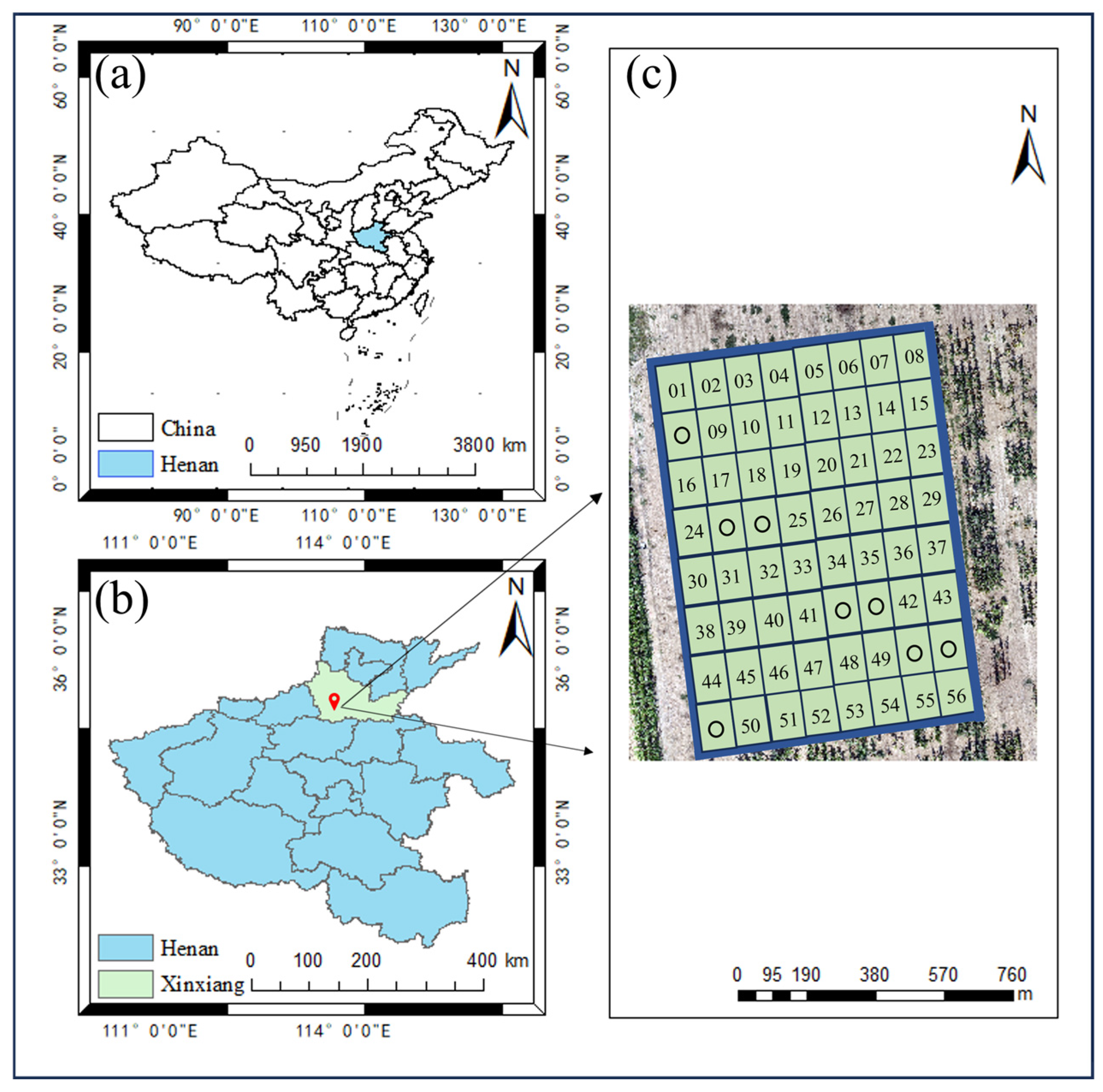
2.1. Overview of the Study Area

The experimental site is located at the Xinxiang Comprehensive Experimental Base of the Chinese Academy of Agricultural Sciences, Xinxiang City, Henan Province (113°45′42″ E, 35°08′05″ N). This region is characterized by a temperate continental monsoon climate, with an average annual rainfall of approximately 500 mm. The abundant summer rainfall creates an ideal environment for maize cultivation. The soil in the experimental area is classified as light loam, and irrigation is conducted using large-scale center-pivot sprinklers. The experiment comprised 56 plots, and each plot had dimensions of 3 m × 2 m, with a row spacing of 0.6 m and a plant spacing of 0.25 m. The layout of the experimental plots is illustrated in Figure 1.

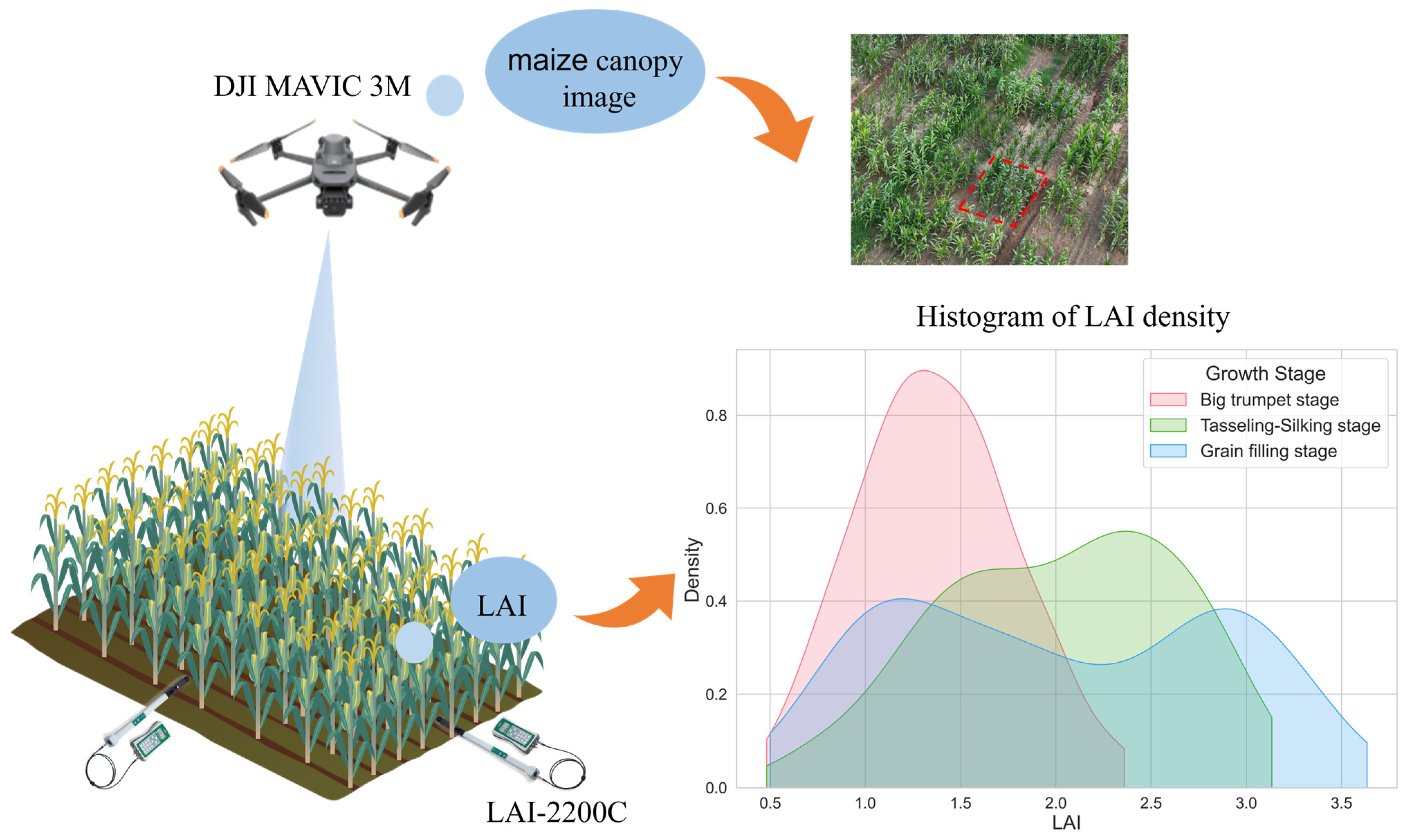
2.2. Data Acquisition

2.2.1. Field Data Acquisition

Data collection was conducted during critical growth stages of maize, such as the big trumpet stage, tasseling–silking, and grain filling stages, through a combination of UAV imagery and field instrument measurements. Meanwhile, the BBCH scale and description [14] corresponding to the three periods are shown in

Table 1. The BBCH scale and description of the relevant phenological stage of maize.

Phenology Stage	BBCH Scale	Description
Principal growth stage 3: stem elongation	39	Nine or more nodes detectable
Principal growth stage 5: inflorescence emergence, heading	51	Beginning of tassel emergence: tassel detectable at top of stem
Principal growth stage 6: flowering, anthesis	61	Male: stamens in middle of tassel visible Female: tip of ear emerging from leaf sheath
Principal growth stage 7: development of fruit	71	Beginning of grain development: kernels at blister stage, approximately 16% dry matter

. Ground-level LAI data were collected using the LAI-2200C Plant Canopy Analyzer (LI-COR, USA), hereafter referred to as measured LAI. Three measurements were obtained from various positions within each plot, spanning both horizontal and vertical directions, and the plot’s LAI was determined by averaging the recorded measurements. For each growth stage, data collection was conducted on a single day. A summary of the statistical information of the maize LAI parameters is presented in

Table 2. Statistics of LAI parameters of maize at different growth stages.

Growth Stages	Data	Sample Size	Leaf Area Index (LAI)
			Min	Max	Mean	Standard Deviation
Big trumpet stage	25 July 2024	56	0.48	2.36	1.46	0.43
Tasseling–silking stage	5 August 2024	56	0.50	2.42	1.59	0.47
Grain filling stage	20 August 2024	56	0.47	2.19	1.30	0.39

.

2.2.2. Acquisition and Preprocessing of UAV Remote Sensing Data

This study utilized the DJI Mavic 3M UAV (SZ DJI Technology Co., Shenzhen, China) to collect aerial data on the same day as ground data collection. The visible light camera equipped on this model has a sensor size of 17.3 mm × 13.0 mm, a resolution of 5280 × 3956 pixels, 20 million effective pixels, and an equivalent focal length of 24 m. The multispectral camera features a 5-megapixel effective resolution and an equivalent focal length of 25 mm. It captures spectral data across four bands: Green (G: 560 ± 16 nm), Near-Infrared (NIR: 860 ± 26 nm), Red Edge (RE: 730 ± 16 nm), and Red (R: 650 ± 16 nm).

The DJI Mavic 3M UAV was deployed for low-altitude flights at 5 m above ground level over the experimental area to acquire RGB images for model development. For the collection of multispectral imagery used in vegetation index calculation, flight missions were planned using DJI Pilot 2 software (SZ DJI Technology Co., Shenzhen, China). The camera was maintained in a nadir orientation, and the flight altitude was set at 30 m above ground level. Both the forward and side overlap rates were configured at 80%, ensuring high-quality image mosaicking and accurate feature identification. To minimize the influence of solar angle on image quality, data acquisition was conducted under clear and windless weather conditions. All UAV flights were scheduled between 11:00 a.m. and 2:00 p.m. Beijing time, corresponding to the period of relatively high and stable solar elevation, which helps reduce shadow effects and ensures consistent illumination across the study area, as shown in Figure 2.

After completing the UAV flight missions, the multispectral images were stitched using Pix4Dmapper 4.5.6 (Pix4D, Lausanne, Switzerland) to generate orthomosaic images. The image processing workflow included key steps such as importing ground control points (GCPs), image registration, alignment, dense point cloud generation, and radiometric correction. Subsequently, ArcGIS 10.6 (Environmental Systems Research Institute, Redlands, CA, USA) was used to georeferenced UAV images acquired at different growth stages. Vegetation indices were extracted by delineating polygon vectors for each plot.

2.2.3. Vegetation Indices Extraction

Vegetation indices are derived by combining data from various spectral bands to emphasize vegetation characteristics and objectively differentiate between vegetation and soil [15]. It effectively reduces the impact of factors like land surface types, and atmospheric conditions on vegetation reflectance, facilitating precise monitoring of subtle variations in maize biochemical markers [16,17]. Building on previous studies [18,19,20,21,22,23,24,25,26,27,28,29,30,31,32,33,34,35,36,37,38], this study identified and computed various vegetation indices, with the corresponding formulas listed in

Table 3. List of vegetation indices (VIs) considered for analysis, their formula, and their source.

VI	Formula	Source
Normalized difference vegetation index (NDVI)	$(\mathrm{NIR}-\mathrm{R})/(\mathrm{NIR}+\mathrm{R})$	[18]
Renormalized difference vegetation index (RDVI)	$(\mathrm{NIR}-\mathrm{R})/\sqrt{(\mathrm{NIR}+\mathrm{R})}$	[19]
Excess green index (ExG)	$2\ast \mathrm{G}-\mathrm{R}-\mathrm{B}$	[20]
Kernel normalized difference vegetation index (kNDVI)	$\tanh \left({\left({\displaystyle \frac{\mathrm{N}\mathrm{I}\mathrm{R}-\mathrm{R}}{2\sigma }}\right)}^2\right)$	[21]
Ratio vegetation index (RVI)	$\mathrm{NIR}/\mathrm{R}$	[22]
Optimization of soil regulatory vegetation index (OSAVI)	$1.16\ast \left[(\mathrm{NIR}-\mathrm{R})/(\mathrm{NIR}+\mathrm{R}+0.16)\right]$	[23]
Modified ratio vegetation index (MSR)	$(\mathbf{N}\mathbf{I}\mathbf{R}/\mathbf{R}-\mathbf{1})\mathbf{S}\mathbf{Q}\mathbf{R}\mathbf{T}(\mathbf{N}\mathbf{I}\mathbf{R}/\mathbf{R}+\mathbf{1})$	[24]
Modified greenness ratio vegetation index (MSR_G)	$(\mathbf{N}\mathbf{I}\mathbf{R}/\mathbf{G}-\mathbf{1})\mathbf{S}\mathbf{Q}\mathbf{R}\mathbf{T}(\mathbf{N}\mathbf{I}\mathbf{R}/\mathbf{G}+\mathbf{1})$	[25]
Nonlinear vegetation index (NLI)	$({\mathrm{N}\mathrm{I}\mathrm{R}}^2-\mathrm{R})/{(\mathrm{N}\mathrm{I}\mathrm{R}}^2+\mathrm{R})$	[26]
Optimal vegetation index (Vlopt)	$1.45\ast ({\mathrm{N}\mathrm{I}\mathrm{R}}^2+1)/(\mathrm{R}+0.45)$	[27]
Red edge normalized difference vegetation index (RENDVI)	$(\mathrm{RE}-\mathrm{R})/(\mathrm{RE}+\mathrm{R})$	[28]
Red edge ratio vegetation index (RESR)	$\mathrm{R}\mathrm{E}/\mathrm{R}$	[29]
Modified nonlinear vegetation index (MNLI)	$1.5({\mathrm{N}\mathrm{I}\mathrm{R}}^2-\mathrm{R})/({\mathrm{N}\mathrm{I}\mathrm{R}}^2+\mathrm{R}+0.5)$	[30]
Wide dynamic range vegetation index (WDRVI)	$(\mathrm{a}\ast \mathrm{NIR}-\mathrm{R})/(\mathrm{a}\ast \mathrm{NIR}+\mathrm{R})$	[31]
Green chlorophyll vegetation index (GCVI)	$\mathrm{N}\mathrm{I}\mathrm{R}/\mathrm{G}-1$	[32]
Modified double-difference vegetation index (MDD)	$\left(\mathrm{N}\mathrm{I}\mathrm{R}-\mathrm{R}\mathrm{E}\right)-(\mathrm{R}\mathrm{E}-\mathrm{G})$	[33]
Modified chlorophyll absorption reflectance index (MCARI1)	$[\left(\mathrm{N}\mathrm{I}\mathrm{R}-\mathrm{R}\mathrm{E}\right)-0.2\ast \left(\mathrm{N}\mathrm{I}\mathrm{R}-\mathrm{R}\right)](\mathrm{N}\mathrm{I}\mathrm{R}/\mathrm{R}\mathrm{E})$	[34]
Modified transformed chlorophyll absorption reflectance index (MTCAR)	$3[\left(\mathrm{N}\mathrm{I}\mathrm{R}-\mathrm{R}\mathrm{E}\right)-0.2\ast \left(\mathrm{N}\mathrm{I}\mathrm{R}-\mathrm{R}\right)](\mathrm{N}\mathrm{I}\mathrm{R}/\mathrm{R}\mathrm{E})$	[35]
Difference vegetation index (DVI)	$\mathrm{NIR}-\mathrm{R}$	[36]
Soil-adjusted vegetation index (SAVI)	$(\mathrm{N}\mathrm{I}\mathrm{R}-\mathrm{R})(1+\mathrm{l})/(\mathrm{N}\mathrm{I}\mathrm{R}+\mathrm{R}+\mathrm{l})(\mathrm{l}=0.5)$	[37]
Modified soil-adjusted vegetation index (MSAVI2)	$(2\ast \mathrm{N}\mathrm{I}\mathrm{R}+1-\mathrm{S}\mathrm{Q}\mathrm{R}\mathrm{T}({\left(2\ast \mathrm{N}\mathrm{I}\mathrm{R}+1\right)}^2-8\ast (\mathrm{N}\mathrm{I}\mathrm{R}-\mathrm{R})\left)\right)/2$	[38]

a = 0.12, $\sigma$ = 0.5(NIR + R). R: red band reflectivity; G: green band reflectivity; B: blue band reflectivity; NIR: near-infrared band reflectivity.

.

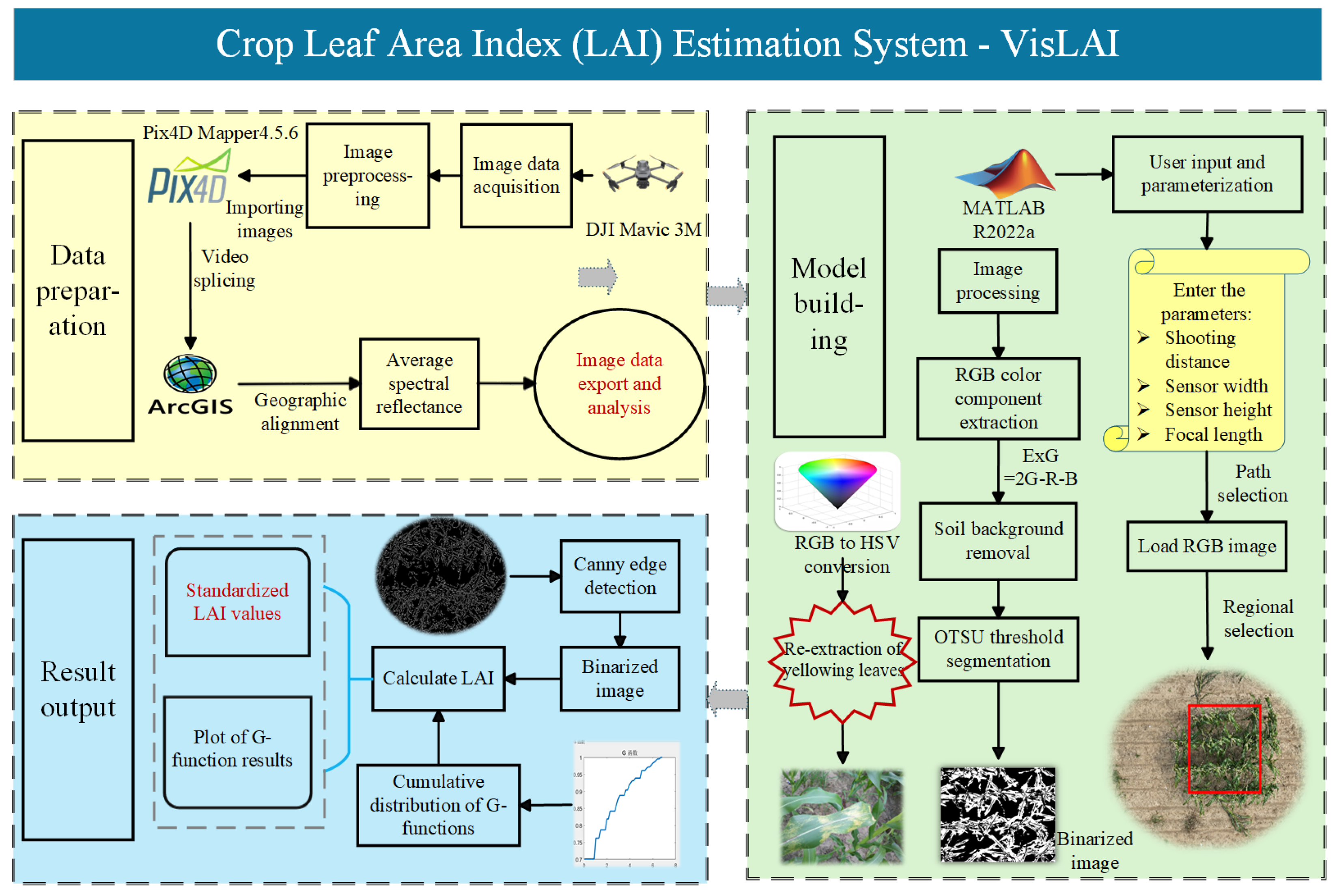
2.3. Image Processing Principles and Methods

2.3.1. Principles of Image Processing

Image analysis technology is an advanced technique that leverages digital image processing and computer vision. It enhances information and extracts key features through the processing and analysis of image data [39]. A digital image consists of numerous pixels, and the representation and encoding of these pixels are essential elements in image analysis [40]. Therefore, by calculating the physical area represented by each pixel, the actual leaf area can be estimated by counting the pixels corresponding to the leaf in the image.

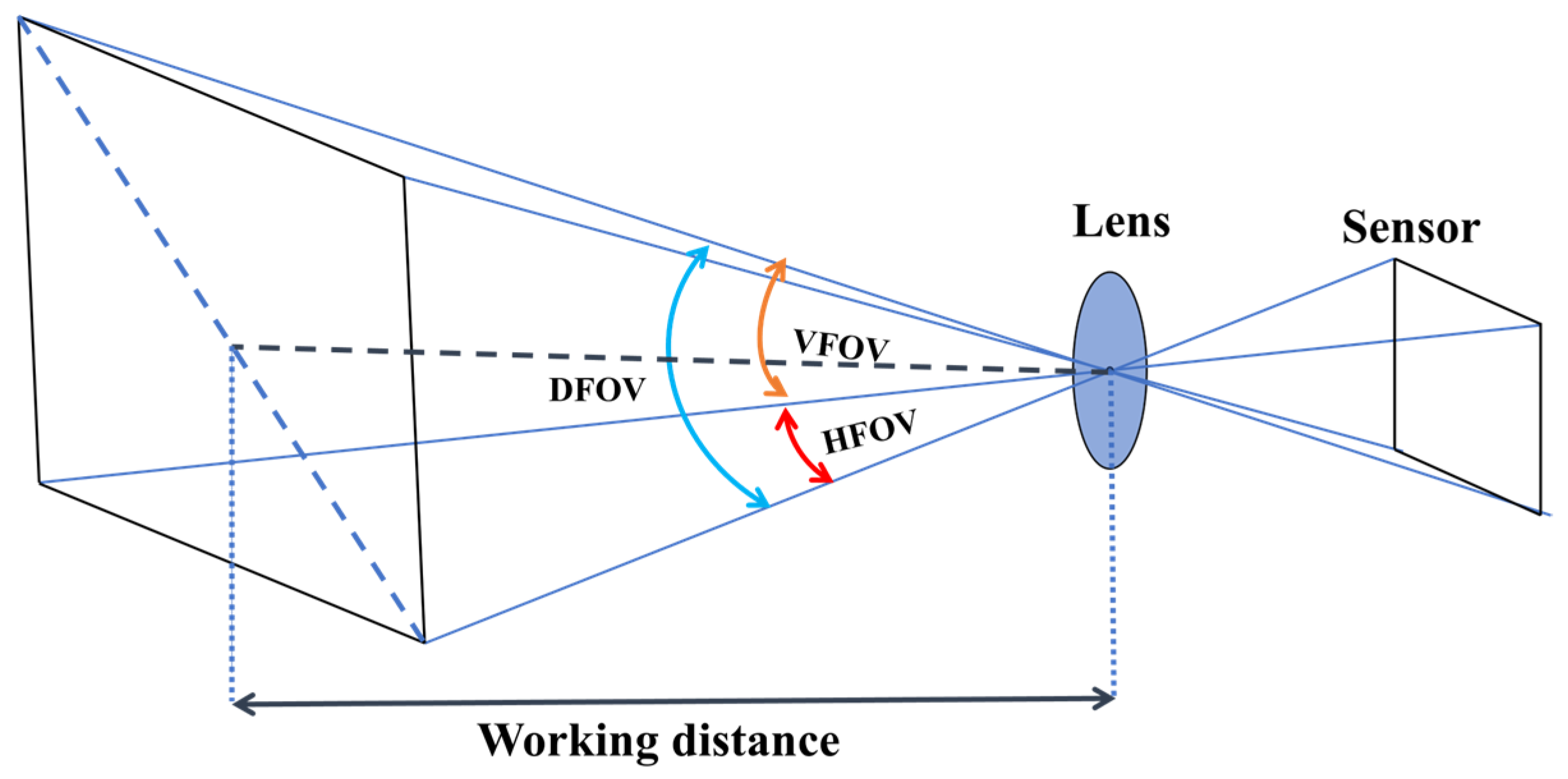
2.3.2. Determining the Actual Size of the Cell Based on the Field of View Angle

Accurate calculation of the actual leaf area of maize requires consideration of the field of view (FOV), as it influences both the range of leaves captured by the camera and the assessment of lighting conditions. FOV is determined by the lens focal length and the size of the image sensor [41]. By considering the distance between the object and the camera, the pixel size in the image can be estimated, which enables the calculation of the plot dimensions, as illustrated in Figure 3.

2.3.3. Segmentation Method Based on RGB and HSV Images

Image segmentation is a crucial preprocessing step in image recognition and computer vision. By extracting regions of interest, it enhances analysis efficiency and provides a foundation for feature extraction and subsequent applications [42]. The OTSU algorithm, also known as Otsu’s method, is a widely used global thresholding technique for image binarization, introduced by Otsu [43]. The algorithm analyzes the grayscale histogram of the image to select a threshold value K, which divides the image into a foreground and background by maximizing the inter-class variance between the two [44]. A larger inter-class variance indicates a more distinct separation between the foreground and background, thereby improving the accuracy of segmentation.

The definition of the between-class variance of its target O and background B:

$${\mathrm{e}}^2\left(\mathrm{K}\right)={\mathrm{P}}_{\mathrm{O}}{\left(\mu -{{\mu }_o}^{\prime }\right)}^2+{\mathrm{P}}_{\mathrm{b}}{\left(\mu -{{\mu }_{\mathrm{b}}}^{\prime }\right)}^2$$

(1)

In the formula, μ represents the mean grayscale value of the image, μ_ο′ and μ_b′ represent the mean values of the target O and the background B, respectively. When the value of K maximizes e²(K), K is the optimal threshold.

The Excess Green Index (ExG) effectively differentiates vegetation from soil backgrounds in RGB images [45]. Based on the OSTU algorithm, threshold segmentation to separate the maize from the background in an RGB image, generating a grayscale image.

$$\mathrm{E}\mathrm{x}\mathrm{G}=2\mathrm{G}-\mathrm{R}-\mathrm{B}$$

(2)

In the formula, G represents the green component in an RGB image, R represents the red component, while B represents the blue component.

This approach forms the basis of the VisLAI-RGB model, which estimates the LAI using vegetation indices derived exclusively from the RGB color space. To enhance the robustness and accuracy of LAI estimation, we propose an improved model, VisLAI-HSV. Unlike the conventional VisLAI-RGB model—which relies solely on RGB-based indices (ExG)—the VisLAI-HSV model integrates additional spectral information by transforming RGB images into the hue–saturation–value (HSV) color space. This transformation improves segmentation and feature extraction, particularly under varying illumination conditions and across different phenological stages of maize.

Compared to the RGB model, the hue–saturation–value (HSV) model more closely aligns with human color perception, making it better suited for color contrast and object segmentation [46]. In image processing, the HSV model effectively separates color information, enhancing the stability of object detection. It is particularly useful in monitoring the transition of maize leaves from green to yellow, aiding in the assessment of plant growth and health [47].

Converting from the RGB color model to the HSV model requires calculating the RGB values of each pixel to determine the corresponding hue, saturation, and value [48], the corresponding conversion formula is as follows:

$$\mathrm{V}=\max \left(\mathrm{R},\mathrm{G},\mathrm{B}\right)$$

(3)

$$\mathrm{S}=\left\{\begin{array}{cc}\hfill {\displaystyle \frac{\mathrm{V}-\min \left(\mathrm{R},\mathrm{G},\mathrm{B}\right)}{\mathrm{V}}},& \mathrm{V}\ne 0\\ \hfill 0,& \mathrm{other}\end{array}\right.$$

(4)

$$\mathrm{H}=\left\{\begin{array}{cc}\hfill 60\ast {\displaystyle \frac{\mathrm{G}-\mathrm{B}}{\mathrm{V}-\min \left(\mathrm{R},\mathrm{G},\mathrm{B}\right)}},& \hfill \mathrm{V}=\mathrm{R}\\ \hfill 120+60\ast {\displaystyle \frac{\mathrm{B}-\mathrm{R}}{\mathrm{V}-\min \left(\mathrm{R},\mathrm{G},\mathrm{B}\right)}},& \hfill \mathrm{V}=\mathrm{G}\\ \hfill 240+60\ast {\displaystyle \frac{\mathrm{R}-\mathrm{G}}{\mathrm{V}-\min \left(\mathrm{R},\mathrm{G},\mathrm{B}\right)}},& \hfill \mathrm{V}=\mathrm{B}\end{array}\right.$$

(5)

In the formula, R: red band reflectivity; G: green band reflectivity; B: blue band reflectivity.

2.3.4. Edge Detection Based on the Canny Algorithm

The Canny edge detection algorithm, proposed by John F. Canny in 1986, is a multi-stage method for edge detection that effectively extracts valuable structural information from images [49]. It is widely employed in various computer vision systems. The algorithm begins with image smoothing using Gaussian filtering to remove noise, followed by the calculation of the image gradient. The magnitudes and directions of the gradient along the horizontal and vertical axes are then determined through differential operations. Edge refinement is achieved through non-maximum suppression, and a dual-thresholding technique is utilized to eliminate false edges while retaining true edges. The final processed image is then output [50]. The algorithm is distinguished by its simplicity and efficiency, effectively detecting edges in an image with a low error rate, while minimizing the influence of noise on the edge detection process.

2.3.5. The Standardized Estimation of LAI Based on the G Function

In image processing, the G function represents an application of the cumulative distribution function (CDF). By providing information on the distribution of leaf area density across various distance ranges, it mitigates biases arising from variations in field of view or observation conditions, thereby enabling the standardized calculation of the LAI [51].

$$\mathrm{G}\left(\mathrm{d}\right)={\displaystyle \frac{\sum _{\mathrm{i}=1}^{\mathrm{j}}\mathrm{h}\mathrm{i}\mathrm{s}\mathrm{t}\left(\mathrm{i}\right)}{\sum _{\mathrm{i}=1}^{\mathrm{N}}\mathrm{h}\mathrm{i}\mathrm{s}\mathrm{t}\left(\mathrm{i}\right)}}$$

(6)

In the formula, d represents the distance, hist(i) denotes the count of the i-th bin in the histogram, and N is the total count.

Based on the above concepts, this paper proposes a method for the identification and extraction of LAI using computer vision techniques. The proposed method integrates UAV-based remote sensing imagery and processes multiple digital images, thereby enabling more accurate estimations of plant leaf area. By employing techniques such as image segmentation, feature extraction, color space transformation, and edge detection, the method effectively identifies and extracts the plant’s leaf area, facilitating the calculation of its surface area. Additionally, the approach incorporates adjustments to FOV and auxiliary calculations utilizing the G function. This ensures standardized processing under various conditions, thereby enhancing the accuracy and comparability of LAI estimates, while also demonstrating robustness across different scenarios.

Figure 4 illustrates the experimental workflow of this study. In this process, the OTSU algorithm is utilized for threshold segmentation, while the ExG Index is employed to differentiate vegetation from the background. The HSV color space is used to monitor leaf chlorosis, and Canny edge detection aids in the precise extraction of leaf contours. Finally, the G function is applied to normalize the calculation of the LAI. Given VisLAI’s ability to efficiently and accurately estimate the LAI under complex conditions, it offers a valuable technical reference for advancing the development of smart agriculture.

2.4. Data Analysis and Evaluation

2.4.1. Construction of Machine Learning-Based Model for Inversion of LAI

This study utilizes multispectral remote sensing data to develop inversion models for an LAI based on vegetation indices such as the NDVI and EVI. Using the LAI-2200C observation protocol, a correlation was established between the vegetation indices derived from UAV-based multispectral remote sensing observations. Furthermore, the study investigates the dynamic changes in the LAI at the field scale, facilitating the rapid assessment of maize growth through the integration of canopy analysis with UAV spectral technology. Pearson correlation analysis was employed to identify the independent variables most strongly correlated with the dependent variable. To enhance the stability and robustness of the model, the dataset was divided into a training set (80%) and a testing set (20%). Six machine learning algorithms—Gradient Boosting (GB), Ridge Regression (RR), Lasso Regression (Lasso), Linear Regression (LR), SVR, and RF—were employed to construct LAI inversion models for different growth stages.

LR is a widely used statistical method for modeling the quantitative relationships between variables. It predicts the value of the target variable by identifying the optimal linear relationship between the independent and dependent variables [52,53]. RR is an improved version of Linear Regression that reduces model overfitting by adding a regularization term to the ordinary least squares (OLS) regression. This regularization term constrains the magnitude of the model parameters, thereby improving the model’s performance on new, unseen data. RR is particularly effective in addressing multicollinearity, a common issue in many research contexts [54]. Lasso achieves regularization by applying a penalty function that shrinks the coefficients of the variables in the regression model, thereby preventing overfitting and mitigating issues of severe multicollinearity [55]. RF constructs a forest composed of numerous decision trees built in a random manner, where the trees are independent of each other. Each decision tree generates a prediction, and the final prediction for the observed data is obtained by averaging all the individual predictions [56]. SVR is a prominent technique for addressing regression problems, where the prediction speed is directly related to the sparsity of support vectors [57]. GB is an ensemble learning method that combines multiple weak classifiers or regressors to form a strong classifier or regressor, thereby enhancing predictive performance. The core idea of the GB algorithm is to use the negative gradient of the loss function as an approximation of the residuals. A base learner is then trained to fit these residuals, and its predictions are added to the previous model, iteratively reducing the value of the loss function [58].

To enhance the performance of LAI prediction, a grid search approach is adopted within the vegetation index inversion framework to determine the most effective set of hyperparameters for the six regression models. Each iteration of the grid search incorporates five-fold cross-validation to evaluate the generalizability of the model. This method involves partitioning the dataset into multiple subsets, allowing for a robust assessment of model stability and reliability. Following the tuning process, the optimized models were employed to estimate the LAI across different developmental stages of summer maize.

2.4.2. Construction of LAI Inversion Model Based on Machine Vision

This study developed an automatic estimation model for LAI extraction (VisLAI) based on UAV remote sensing imagery and computer vision technology. By applying median filtering to denoise the image, the RGB color space components are extracted. The ExG and Otsu algorithms are used for thresholding, generating a binarized ExG image. To further improve the accuracy of leaf region identification, the RGB image is converted to the HSV color space, effectively capturing yellowing leaves at different growth stages. This is combined with the initial segmentation results to generate a new binary image. Simultaneously, the Canny edge detection algorithm and the cumulative distribution function (CDF) are used to standardize the calculation of leaf area.

The model uses low-altitude UAV-acquired imagery of individual plots as input to estimate the leaf area index (LAI), and the predicted results are compared with ground-truth measurements obtained using the LAI-2200C plant canopy analyzer.

2.4.3. Model Accuracy Evaluation

This study employs the coefficient of determination (R²), root mean square error (RMSE), and normalized root mean square error (NRMSE) as metrics for assessing the model’s accuracy. A value of R² closer to 1 indicates a better fit of the model to the data. Lower values of RMSE and NRMSE correspond to higher accuracy in the model’s predictions.

$${\mathrm{R}}^{2 }={\displaystyle \frac{{(\sum _{\mathrm{i}=1}^{\mathrm{n}}{\mathrm{y}}_{\mathrm{i}}-\stackrel{\mathrm{-}}{ \mathrm{y}})}^2}{{(\sum _{\mathrm{i}=1}^{\mathrm{n}}{\mathrm{x}}_{\mathrm{i}}-\stackrel{\mathrm{-}}{\mathrm{y}})}^2}}$$

(7)

$$\mathrm{RMSE}=\sqrt{{\displaystyle \frac{\sum _{\mathrm{i}=1,\mathrm{j}=1}^{\mathrm{n}}{({\mathrm{x}}_{\mathrm{i} }-{\mathrm{y}}_{\mathrm{j}})}^2}{\mathrm{n}}}}$$

(8)

$$\mathrm{NRMSE}={\displaystyle \frac{\mathrm{RMSE}}{{\mathrm{y}}_{\mathrm{m}\mathrm{a}\mathrm{x}}-{\mathrm{y}}_{\mathrm{m}\mathrm{i}\mathrm{n}}}}$$

(9)

In the formula, ${\mathrm{x}}_{\mathrm{i}}$ represents the observed LAI values of maize, ${\mathrm{y}}_{\mathrm{i}}$ denotes the estimated LAI values of maize, i and j are sample identifiers, n is the total number of samples, and $\stackrel{\mathrm{-}}{\mathrm{y}}$ is the mean of the observed values.

3. Results

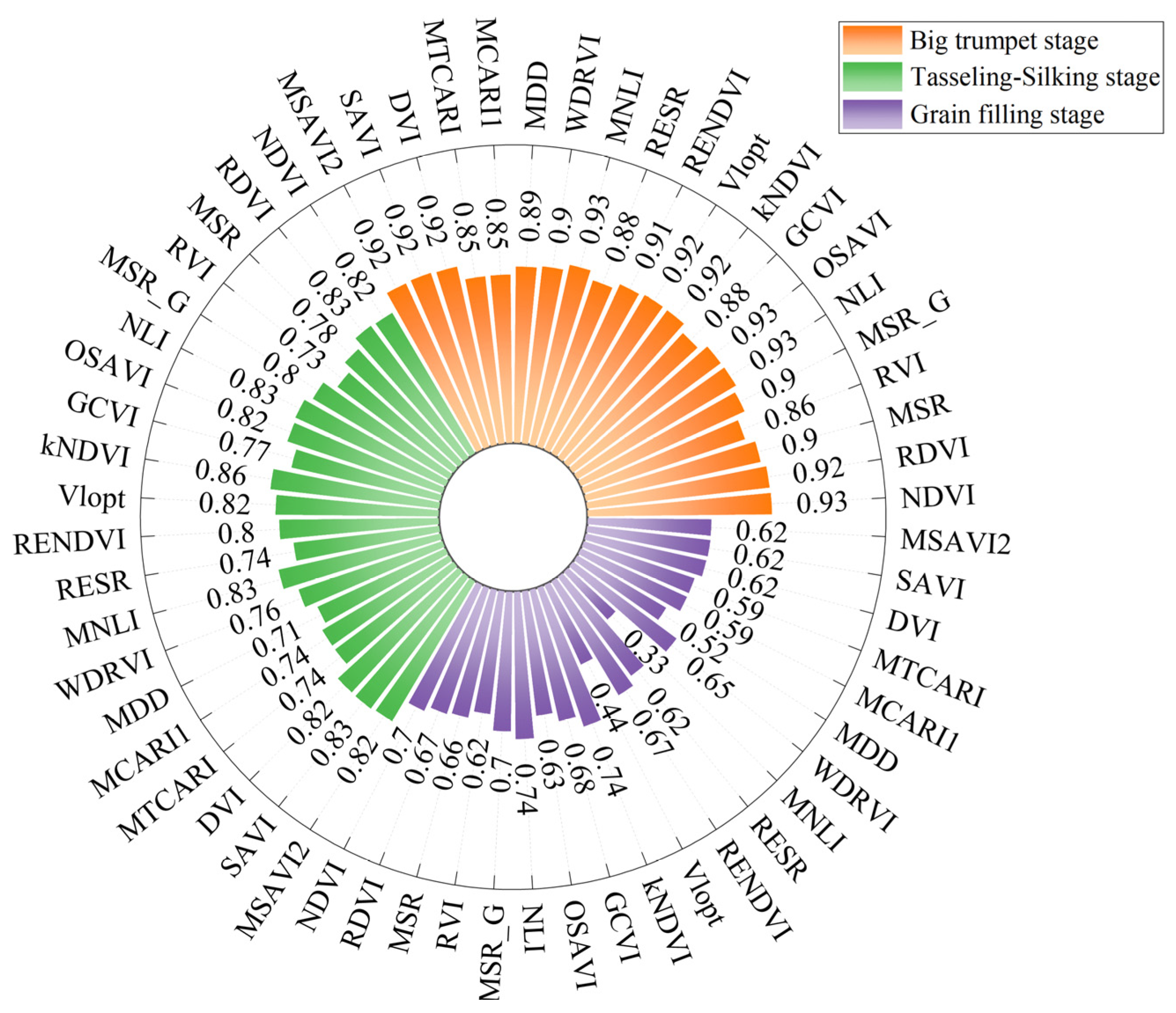
3.1. Correlation Analysis

The correlation analysis between vegetation indices at various growth stages and the LAI values measured by the LAI-2200C plant canopy analyzer is presented in Figure 5. The Pearson correlation coefficients between the selected vegetation indices and the measured LAI during the big trumpet stage range from 0.85 to 0.93, whereas the coefficients during the tasseling–silking and grain filling stages range from 0.71 to 0.86 and 0.33 to 0.74, respectively. Based on the correlations between the vegetation indices and the measured LAI across different growth stages, the top 20 vegetation indices—such as NDVI, RDVI, MSR, RVI, MSR-G, NLI, OSAVI, GCVI, kNDVI, RENDVI, RESR, WDRVI, MDD, MCARI1, MRETVI, MTCARI, DVI, SAVI, and MSAVI2—demonstrating the most optimal performance were selected as input variables. The measured LAI values served as the output variable. Subsequently, six machine learning algorithms—LR, RR, Lasso, RF, SVR, and GB—were employed to develop LAI inversion models for summer maize across different growth stages.

The correlation coefficient between the LAI estimated by VisLAI and the measured LAI during the big trumpet stage is 0.95, while the coefficients for the tasseling–silking and grain filling stages are 0.93 and 0.92, respectively. These results indicate a strong correlation between the LAI of summer maize estimated by VisLAI and the observed LAI across different growth stages.

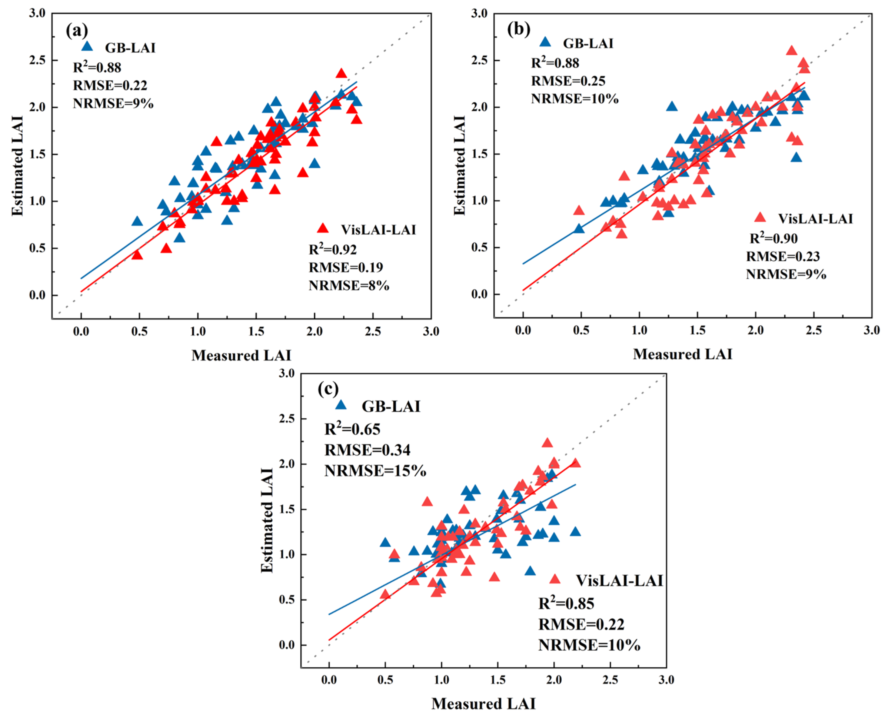
3.2. Comparison of Accuracy Across Different Estimation Models

LAI inversion for summer maize was conducted using six distinct machine learning algorithms, with the inversion accuracy results presented in

Table 4. Estimation accuracy of maize LAI using different machine learning algorithms.

Machine Learning	Growth Stages	Big Trumpet Stage			Tasseling–Silking Stage			Grain Filling Stage
	Metric	R2	RMSE	NRMSE (%)	R2	RMSE	NRMSE (%)	R2	RMSE	NRMSE (%)
GB	Training set	0.94	0.15	6%	0.90	0.21	9%	0.89	0.18	8%
	Test set	0.82	0.26	16%	0.78	0.34	15%	0.78	0.28	15%
LR	Training set	0.90	0.20	8%	0.79	0.31	13%	0.69	0.30	14%
	Test set	0.79	0.28	17%	0.55	0.48	21%	0.59	0.38	20%
RR	Training set	0.87	0.22	9%	0.74	0.34	14%	0.52	0.38	17%
	Test set	0.78	0.29	17%	0.68	0.41	18%	0.60	0.37	20%
Lasso	Training set	0.85	0.24	10%	0.74	0.34	14%	0.47	0.40	18%
	Test set	0.79	0.28	17%	0.72	0.38	16%	0.54	0.40	21%
RF	Training set	0.90	0.19	8%	0.80	0.30	12%	0.84	0.21	10%
	Test set	0.81	0.27	16%	0.75	0.36	15%	0.71	0.32	17%
SVR	Training set	0.88	0.21	9%	0.74	0.34	14%	0.61	0.34	15%
	Test set	0.80	0.27	16%	0.70	0.40	17%	0.67	0.34	18%

. The models exhibited lower predictive accuracy during the grain filling stage, while higher accuracy was observed during the big trumpet and tasseling–silking stages. This pattern aligns with the variations in the correlation of individual vegetation indices, thereby further validating the robustness of the model construction.

As presented in Table 4, when evaluating the inversion performance across the three growth stages, the model constructed using the GB algorithm demonstrates the best overall performance. During the big trumpet, tasseling–silking, and grain filling stages, the R² of the GB algorithm on the test set ranged from 0.78 to 0.82. In comparison, the R² for LR, RR, Lasso, RF, and SVR were marginally lower than those of the GB. Furthermore, the corresponding RMSE (0.26–0.34) and NRMSE (15–16%) for the GB algorithm were consistently lower than those observed for the other models. In conclusion, the model built using the GB algorithm outperforms all other models across the three growth stages and is therefore selected for LAI prediction.

The R² for the VisLAI model based on visible light imagery during the big trumpet, tasseling–silking, and grain filling stages are 0.84, 0.75, and 0.50, respectively, with corresponding RMSE values of 0.24, 0.35, and 0.44. In contrast, the R² for the HSV-optimized VisLAI are 0.92, 0.90, and 0.85, with RMSE values of 0.19, 0.23, and 0.22. The accuracy of the HSV-optimized VisLAI model significantly outperforms that of the VisLAI model based solely on visible light imagery, particularly during the grain filling stage, where the R² improved by 0.08, 0.15, and 0.35, and the RMSE decreased by 0.05, 0.12, and 0.22, respectively. These results indicate that the HSV-optimized VisLAI model is more effective at accurately identifying yellowing leaves and enhancing the precision of LAI estimation. The estimation accuracy of maize LAI using both the VisLAI model based on visible light imagery and the HSV-optimized VisLAI model is summarized in

Table 5. Estimation accuracy of two methods for extracting maize LAI.

Method	Big Trumpet Stage			Tasseling–Silking Stage			Grain Filling Stage
	R2	RMSE	NRMSE (%)	R2	RMSE	NRMSE (%)	R2	RMSE	NRMSE (%)
VisLAI-RGB	0.84	0.24	14%	0.75	0.35	14%	0.50	0.44	23%
VisLAI-HSV	0.92	0.19	8%	0.90	0.23	9%	0.85	0.22	10%

.

The regression plots of the maize LAI predicted for all plots during the big trumpet, tasseling–silking, and grain filling stages, using the more accurate VisLAI model (VisLAI-HSV) and the GB algorithm, are presented in Figure 6. The R² of the vegetation indices inversion model during the big trumpet stage, tasseling–silking stage, and grain filling stage are 0.88, 0.88, and 0.65, respectively. The corresponding RMSE values are 0.22, 0.25 and 0.34, while the NRMSE values are 9%, 10%, and 15%, respectively. The estimation results from the vegetation indices inversion model indicate that R² is highest during the big trumpet stage and tasseling–silking stage. At the same time, the RMSE and NRMSE are smallest during the big trumpet stage.

The accuracy analysis of the VisLAI-predicted summer maize LAI and the measured LAI is presented in Figure 6. R² is highest during the big trumpet stage, reaching 0.92, followed by the tasseling–silking stage and the grain filling stage, with R² values of 0.90 and 0.85, respectively. The RMSE is lowest during the big trumpet stage, at 0.19, while it is 0.23 for both the tasseling–silking and grain filling stages. Similarly, the NRMSE is also minimal during the big trumpet stage, with a value of 3%, compared to 9% and 10% for the tasseling–silking and grain filling stages, respectively. During the big trumpet, tasseling–silking, and grain filling stages of summer maize, the LAI estimated by VisLAI demonstrates higher accuracy and smaller errors compared to the LAI derived from the vegetation indices inversion model. Especially during the grain filling stage, R² of the LAI estimated by VisLAI is significantly higher than that of the LAI derived from the vegetation indices inversion model, while the accuracy of the vegetation indices inversion-based LAI is the lowest during the grain filling stage.

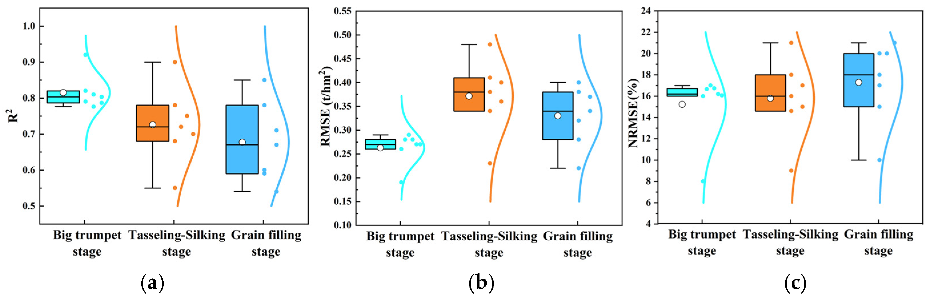
3.3. Changes in Model Accuracy at Different Fertility Stages

Figure 7 illustrates the accuracy of LAI estimation by different models across various growth stages. The results highlight the differing performance of machine learning-based algorithms and the VisLAI model, which utilizes UAV imagery and computer vision techniques, in estimating maize LAI during the three growth stages. During the big trumpet stage, R² values range from 0.78 to 0.92, with RMSE ranging from 0.19 to 0.29 and NRMSE ranging from 8% to 17%. In the tasseling–silking stage, R² values range from 0.55 to 0.90, with RMSE ranging from 0.23 to 0.48 and NRMSE ranging from 9% to 21%. During the grain filling stage, R² values range from 0.54 to 0.85, with RMSE ranging from 0.22 to 0.40 and NRMSE ranging from 10% to 21%. The results highlight that, compared to the grain filling and tasseling–silking stages, the models exhibit superior performance during the big trumpet stage, demonstrating their capacity to provide more accurate and precise LAI estimates.

3.4. Spatial Distribution of LAI in Summer Maize

Figure 8 presents the LAI distribution maps for the three growth stages of maize, based on the optimal LAI estimation model (VisLAI). The results of this study indicate that, as maize progresses through its growth stages, the LAI values generally show an initial increase, followed by a subsequent decrease. The average LAI during the big trumpet stage is 1.22, during the tasseling–silking stage is 1.32, and during the grain filling stage is 1.07. During the big trumpet stage, maize experiences rapid growth, with the LAI exhibiting a sharp upward trend, peaking at this stage. As maize enters the grain filling stage, physiological senescence processes such as chlorophyll degradation and reduced photosynthetic activity begin to occur in the leaves. This leads to gradual leaf aging and noticeable shrinkage, leading to a decline in the LAI.

4. Discussion

4.1. Comparison of Different Machine Learning Algorithms

Different machine learning algorithms exhibit varying levels of performance in predicting the LAI of summer maize. GB outperforms all other models, followed by RF. The nonlinear regression model demonstrates significantly higher accuracy than the LR model, as remote sensing data often reveal complex, nonlinear relationships with biomass [17]. LR methods, which rely on linear assumptions, perform poorly in this context because they cannot effectively capture the nonlinear characteristics of the data during the fitting process, resulting in lower prediction accuracy [59]. In contrast, decision tree-based ensemble learning methods exhibit strong robustness and stability when handling high-dimensional data and complex nonlinear relationships.

RF and GB models, by integrating multiple decision trees, progressively mitigate overfitting and enhance the model’s generalization ability, resulting in higher prediction accuracy. In contrast, LR and RR models exhibit relatively poor performance in remote sensing data processing, primarily due to their assumption of a linear relationship between input features and the target variable, which makes it difficult to effectively capture complex nonlinear variations. Additionally, LR is highly sensitive to outliers, which can lead to significant prediction errors in remote sensing data. Although RR reduces overfitting through regularization, it still struggles to capture nonlinear relationships effectively, leading to generally inferior performance compared to decision tree-based ensemble learning methods. SVR models, while effective for certain problems [60], are sensitive to the choice of parameters and kernel functions. When handling complex nonlinear relationships, SVR models tend to be less robust than ensemble learning methods. Comparative analysis demonstrates that decision tree-based ensemble learning methods, such as GB and RF, offer a significant advantage in remote sensing data inversion for LAI estimation. These methods excel at handling nonlinear relationships, resulting in higher accuracy and greater robustness.

4.2. LAI Estimation of Summer Maize Based on VisLAI

With the continuous advancements in computer technology, VisLAI has demonstrated exceptional performance in handling dynamic datasets and real-time processing tasks, underscoring its robust adaptability and flexibility. Dorj et al. [61] utilized image processing to estimate citrus orchard yields through fruit detection and counting. Niu et al. [62] fixed fisheye cameras in maize, soybean, and caragana plots to regularly capture canopy images and utilized image processing software to analyze the data and estimate the LAI. While considerable research has been conducted on estimating the LAI, studies focused on enhancing the accuracy of LAI estimation through soil-adjusted vegetation indices, such as the ExG Index, HSV re-extraction, and modifications to the aggregation index G function, remain relatively limited. The ExG Index is widely used as it effectively differentiates between vegetation and soil, demonstrating a strong correlation with the LAI across all three growth stages. However, ExG images often contain erroneous data due to stray light or shadows, especially when the boundary between soil and vegetation is unclear. The application of median filtering for denoising and Gaussian filtering for smoothing proves effective in removing such noise, thereby improving image quality. These findings align with those of Yamaguchi et al. [63].

The conversion from the RGB color space to the HSV color space provides more accurate color information for subsequent image analysis, particularly concerning variations in hue and saturation. At different growth stages, the color of maize leaves undergoes significant changes. During the early growth phase, the plants exhibit healthy leaf development, with the maize leaves in the experimental area fully extended and displaying a vibrant, bright hue. However, as the growth stage progresses, the maize leaves gradually become yellow, showing various shades of brown and reddish-brown. Additionally, the proportion of exposed soil in the experimental area increases. This change forms the theoretical foundation for extracting information from the Hue (H) and Saturation (S) channels in the HSV color space, enabling more precise capture of color variations in the vegetation across different stages. By setting a specific hue range, this study facilitates the re-extraction of leaves exhibiting yellowing and wilting at various growth stages. This method effectively filters out such leaves, thereby improving the accuracy of leaf area estimation. In contrast to the studies by Lu et al. [12] and Niu et al. [62], this research not only focuses on the green portions of the leaves but also incorporates color changes during the leaf senescence stage. This approach enhances the model’s adaptability and accuracy in capturing the various stages throughout the maize’s growth cycle.

4.3. Advantages and Disadvantages of VisLAI Compared to Machine Learning Algorithms

Image processing techniques enable real-time processing of UAV-captured images, facilitating the rapid calculation of the LAI. Through automated image analysis workflows, large-scale image datasets can be processed efficiently, making this approach particularly suitable for the rapid monitoring and assessment of maize growth conditions. Users need only to configure the photography parameters and define the maize ping area to quickly obtain the LAI of the target region. Although vegetation indices-based inversion methods can estimate the LAI with reasonable accuracy, they rely on external data and involve complex data processing. This is especially true when large sample datasets are required, as training the model can be time-consuming. In contrast, image processing methods enable real-time analysis using existing UAV image data, offering greater flexibility and applicability. By integrating ExG, HSV re-extraction, and G-function normalization, the image processing method effectively mitigates interference from soil background, stray light, and leaf degradation, allowing for a clearer distinction between vegetation and background areas, thereby achieving high-precision region extraction. Vegetation indices are typically estimated based on pixel-level averages to assess vegetation growth status. However, during different growth stages, particularly under more complex conditions such as leaf wilting or yellowing, the inversion accuracy of vegetation indices may be compromised. While machine learning methods can improve prediction accuracy, the processes of model training, validation, and tuning require significant time and computational resources. Furthermore, machine learning models may be prone to overfitting or underfitting, necessitating continuous optimization and updates [64]. In contrast, VisLAI demonstrates a distinct advantage in estimating the LAI for summer maize, exhibiting high stability and robustness. It effectively handles environmental disturbances, resulting in superior accuracy.

4.4. Estimation Accuracy of LAI at Different Growth Stages

As the growing season progresses, the R² for both models gradually declines. This decrease can be attributed to the later stages of maize growth, particularly during the maize reproductive phase, when significant changes in leaf color occur, transitioning to yellow [65]. These dynamic variations in leaf color influence the models’ prediction accuracy. During the maturity phase, the complexity of photosynthesis and changes in leaf pigments further reduce the models’ interpretability, leading to a decline in the R² value. The RMSE initially increases before decreasing, with this fluctuation likely resulting from variations in maize growth at different stages, especially during transitional stages when uneven growth rates and biomass distribution introduce errors. During the early and mid-growth stages, maize development is relatively uniform, leading to smaller errors. In contrast, as maize approaches maturity in the later stages, factors such as leaf yellowing [66], biomass changes [65], and increased uncertainty in observational data contribute to higher RMSE values. However, as the model adapts to these changes, error values decrease, resulting in a subsequent reduction in RMSE. The NRMSE shows a gradual increase across the three growth stages. This trend suggests that, as the maize progresses through its growth stages, the model progressively adapts to the dynamic changes, becoming more capable of addressing the complexities and evolving characteristics of the growth process in the later stages.

4.5. The Significance and Limitations of This Study

Image processing technology, with its advantages of real-time performance, automation, and convenience, has been extensively applied in maize information extraction, providing timely and accurate decision support for crop growth monitoring and agricultural management [67]. The LAI of summer maize, as estimated by VisLAI, undergoes median filtering, thresholding, and edge extraction through its built-in image processing toolbox, resulting in high estimation accuracy. However, this method currently addresses only three key growth stages of maize: the big trumpet stage, the tasseling–silking stage, and the grain filling stage, which may not fully capture the dynamic variations across the entire maize growth cycle. To address this limitation, future research should broaden the analysis to encompass image data from the entire maize growth cycle, incorporating dynamic change analysis based on time-series data to more accurately capture the temporal variations in crop development. Additionally, the degree of leaf yellowing or wilting varies significantly across maize cultivars, highlighting the importance of validating the model across multiple maize varieties [68]. While the VisLAI model primarily relies on static image processing techniques, which are susceptible to variations in image quality and external environments, and its robustness needs to be improved. To enhance the model’s adaptability in complex environments, subsequent research can introduce dynamic and adaptive image processing methods, combined with multi-angle image fusion technology, to improve its stability and accuracy.

From a broader application perspective, VisLAI, especially the optimized version of HSV, has good migratory properties and has the potential to be extended to satellite remote sensing platforms. Satellite imagery (e.g., Sentinel-2) currently provides the basis for scaling up from the localized scope of UAVs to regional or even national scales. However, the application of satellite platforms still faces challenges such as scale conversion and low resolution. Under low resolution conditions, the ability of HSV color space to express detailed features such as leaf yellowing may be reduced. Therefore, the future should focus on exploring the adaptation of VisLAI in satellite remote sensing platforms.

5. Conclusions

This study evaluates the accuracy of various methods for estimating the LAI at different growth stages of maize and compares the performance of the VisLAI method with six machine learning algorithms for LAI retrieval. The key conclusions drawn from this study are as follows:

(1) Vegetation indices and the LAI exhibit a strong correlation, with the highest correlation observed during the big trumpet and tasseling–silking stages of maize, and a lower correlation during the grain filling stage. The performance of different machine learning algorithms in estimating maize LAI varies, with the GB algorithm achieving the highest estimation accuracy.

(2) Compared to the VisLAI model based on visible light imagery, the HSV-optimized VisLAI model demonstrates superior accuracy. In cases of crop leaf senescence, the re-extraction of senescent leaves using HSV significantly enhances the precision of VisLAI extraction.

(3) The VisLAI model demonstrates significantly higher accuracy than the machine learning algorithms in estimating maize LAI. The R² for VisLAI at the three growth stages are 0.92, 0.90, and 0.85, respectively, highlighting its superior performance in capturing the variations in maize LAI across different growth phases.

In summary, compared to traditional machine learning algorithms, the VisLAI model demonstrates superior accuracy and robustness in estimating LAI for maize. Its capability to dynamically monitor crop growth provides critical insights, thereby supporting the advancement of precision agriculture.

References

1. Fang, H.L.; Baret, F.; Plummer, S.; Schaepman-Strub, G. An Overview of Global Leaf Area Index (LAI): Methods, Products, Validation, and Applications. Rev. Geophys. 2019, 57, 739–799. [Google Scholar] [CrossRef]
2. Tooley, G.; Nippert, J.B.; Ratajczak, Z. Evaluating methods for measuring the leaf area index of encroaching shrubs in grasslands: From leaves to optical methods, 3-D scanning, and airborne observation. Agric. For. Meteorol. 2024, 349, 109964. [Google Scholar] [CrossRef]
3. He, K.; Du, M.; Tian, X.; Xu, D.; Yin, X.; Li, Z. Effect of Cotton Planting Density on the Estimation of Leaf Area Index Using the LAI-2200 Plant Canopy Analyzer. Crops 2015, 5, 123–127. [Google Scholar] [CrossRef]
4. Zhang, J.J.; Cheng, T.; Guo, W.; Xu, X.; Qiao, H.B.; Xie, Y.M.; Ma, X.M. Leaf area index estimation model for UAV image hyperspectral data based on wavelength variable selection and machine learning methods. Plant Methods 2021, 17, 49. [Google Scholar] [CrossRef]
5. Chatterjee, S.; Baath, G.S.; Sapkota, B.R.; Flynn, K.C.; Smith, D.R. Enhancing LAI estimation using multispectral imagery and machine learning: A comparison between reflectance-based and vegetation indices-based approaches. Comput. Electron. Agric. 2025, 230, 109790. [Google Scholar] [CrossRef]
6. Jin, Z.Y.; Liu, H.Z.; Cao, H.N.; Li, S.L.; Yu, F.H.; Xu, T.Y. Hyperspectral Remote Sensing Estimation of Rice Canopy LAI and LCC by UAV Coupled RTM and Machine Learning. Agriculture 2025, 15, 11. [Google Scholar] [CrossRef]
7. Du, X.Y.; Zheng, L.Y.; Zhu, J.P.; He, Y. Enhanced Leaf Area Index Estimation in Rice by Integrating UAV-Based Multi-Source Data. Remote Sens. 2024, 16, 1138. [Google Scholar] [CrossRef]
8. Xue, W.; Xia, X.Y.; Wan, P.C.; Zhong, P.; Zheng, X. Adversarial Attack on Object Detection via Object Feature-Wise Attention and Perturbation Extraction. Tsinghua Sci. Technol. 2025, 30, 1174–1189. [Google Scholar] [CrossRef]
9. Chen, B.; Wu, Z.; Li, H.; Wang, J. Research of machine vision technology in agricultural application: Today and the future. Sci. Technol. Rev. 2018, 36, 54–65. [Google Scholar]
10. Elinisa, C.A.; Maina, C.W.; Vodacek, A.; Mduma, N. Image Segmentation Deep Learning Model for Early Detection of Banana Diseases. Appl. Artif. Intell. 2025, 39, e2440837. [Google Scholar] [CrossRef]
11. Sun, H.R.; Wei, Z.J.; Yu, W.G.; Yang, G.X.; She, J.N.; Zheng, H.B.; Jiang, C.Y.; Yao, X.; Zhu, Y.; Cao, W.X.; et al. SIDEST: A sample-free framework for crop field boundary delineation by integrating super-resolution image reconstruction and dual edge-corrected Segment Anything model. Comput. Electron. Agric. 2025, 230, 109897. [Google Scholar] [CrossRef]
12. Lu, D.Y.; Jin, Z.J.; Lu, L.; He, W.Z.; Shu, Z.F.; Shao, J.N.; Ye, J.H.; Liang, Y.R. Exploratory study on the image processing technology-based tea shoot identification and leaf area calculation. J. Tea Sci. 2023, 43, 691–702. [Google Scholar]
13. Müller, M.; Casser, V.; Lahoud, J.; Smith, N.; Ghanem, B. Sim4CV: A Photo-Realistic Simulator for Computer Vision Applications. Int. J. Comput. Vis. 2018, 126, 902–919. [Google Scholar] [CrossRef]
14. Feng, Z.; Cheng, Z.; Ren, L.; Liu, B.; Zhang, C.; Zhao, D.; Sun, H.; Feng, H.; Long, H.; Xu, B.; et al. Real-time monitoring of maize phenology with the VI-RGS composite index using time-series UAV remote sensing images and meteorological data. Comput. Electron. Agric. 2024, 224, 109212. [Google Scholar] [CrossRef]
15. Ji, L.; Zhang, L.; Rover, J.; Wylie, B.K.; Chen, X.X. Geostatistical estimation of signal-to-noise ratios for spectral vegetation indices. Isprs J. Photogramm. Remote Sens. 2014, 96, 20–27. [Google Scholar] [CrossRef]
16. Cheng, Q.; Xu, H.; Cao, Y.; Duan, F.; Chen, Z. Grain Yield Prediction of Winter Wheat Using Multi-temporal UAV Based on Multispectral Vegetation Index. Trans. Chin. Soc. Agric. Mach. 2021, 52, 160–167. [Google Scholar]
17. Zhai, W.G.; Li, C.C.; Fei, S.P.; Liu, Y.H.; Ding, F.; Cheng, Q.; Chen, Z. CatBoost algorithm for estimating maize above-ground biomass using unmanned aerial vehicle-based multi-source sensor data and SPAD values. Comput. Electron. Agric. 2023, 214, 108306. [Google Scholar] [CrossRef]
18. Li, X.; Xu, J.W.; Jia, Y.Y.; Liu, S.; Jiang, Y.D.; Yuan, Z.L.; Du, H.Y.; Han, R.; Ye, Y. Spatio-temporal dynamics of vegetation over cloudy areas in Southwest China retrieved from four NDVI products. Ecol. Inform. 2024, 81, 102630. [Google Scholar] [CrossRef]
19. Pullanagari, R.R.; Yule, I.J.; Hedley, M.J.; Tuohy, M.P.; Dynes, R.A.; King, W.M. Multi-spectral radiometry to estimate pasture quality components. Precis. Agric. 2012, 13, 442–456. [Google Scholar] [CrossRef]
20. Perez, O.; Diers, B.; Martin, N. Maturity Prediction in Soybean Breeding Using Aerial Images and the Random Forest Machine Learning Algorithm. Remote Sens. 2024, 16, 4343. [Google Scholar] [CrossRef]
21. Wang, Q.; Moreno-Martinez, A.; Munoz-Mari, J.; Campos-Taberner, M.; Camps-Valls, G. Estimation of vegetation traits with kernel NDVI. Isprs J. Photogramm. Remote Sens. 2023, 195, 408–417. [Google Scholar] [CrossRef]
22. Zhou, Z.J.; Jabloun, M.; Plauborg, F.; Andersen, M.N. Using ground-based spectral reflectance sensors and photography to estimate shoot N concentration and dry matter of potato. Comput. Electron. Agric. 2018, 144, 154–163. [Google Scholar] [CrossRef]
23. Qiao, L.; Tang, W.J.; Gao, D.H.; Zhao, R.M.; An, L.L.; Li, M.Z.; Sun, H.; Song, D. UAV-based chlorophyll content estimation by evaluating vegetation index responses under different crop coverages. Comput. Electron. Agric. 2022, 196, 106775. [Google Scholar] [CrossRef]
24. Zhou, Q.F.; Liu, Z.Y.; Huang, J.F. Detection of nitrogen-overfertilized rice plants with leaf positional difference in hyperspectral vegetation index. J. Zhejiang Univ.-Sci. B 2010, 11, 465–470. [Google Scholar] [CrossRef]
25. Cao, Q.; Miao, Y.X.; Wang, H.Y.; Huang, S.Y.; Cheng, S.S.; Khosla, R.; Jiang, R.F. Non-destructive estimation of rice plant nitrogen status with Crop Circle multispectral active canopy sensor. Field Crops Res. 2013, 154, 133–144. [Google Scholar] [CrossRef]
26. Huang, X.; Lin, D.; Mao, X.M.; Zhao, Y. Multi-source data fusion for estimating maize leaf area index over the whole growing season under different mulching and irrigation conditions. Field Crops Res. 2023, 303, 109111. [Google Scholar] [CrossRef]
27. Chen, R.; Han, L.; Zhao, Y.H.; Zhao, Z.L.; Liu, Z.; Li, R.S.; Xia, L.F.; Zhai, Y.M. Extraction and monitoring of vegetation coverage based on uncrewed aerial vehicle visible image in a post gold mining area. Front. Ecol. Evol. 2023, 11, 1171358. [Google Scholar]
28. Elsayed, S.; Rischbeck, P.; Schmidhalter, U. Comparing the performance of active and passive reflectance sensors to assess the normalized relative canopy temperature and grain yield of drought-stressed barley cultivars. Field Crops Res. 2015, 177, 148–160. [Google Scholar] [CrossRef]
29. Erdle, K.; Mistele, B.; Schmidhalter, U. Comparison of active and passive spectral sensors in discriminating biomass parameters and nitrogen status in wheat cultivars. Field Crops Res. 2012, 124, 74–84. [Google Scholar] [CrossRef]
30. Feng, W.; Wu, Y.P.; He, L.; Ren, X.X.; Wang, Y.Y.; Hou, G.G.; Wang, Y.H.; Liu, W.D.; Guo, T.C. An optimized non-linear vegetation index for estimating leaf area index in winter wheat. Precis. Agric. 2019, 20, 1157–1176. [Google Scholar] [CrossRef]
31. Cao, Y.; Li, G.L.; Luo, Y.K.; Pan, Q.; Zhang, S.Y. Monitoring of sugar beet growth indicators using wide-dynamic-range vegetation index (WDRVI) derived from UAV multispectral images. Comput. Electron. Agric. 2020, 171, 105331. [Google Scholar] [CrossRef]
32. Huang, X.; Vrieling, A.; Dou, Y.; Belgiu, M.; Nelson, A. A robust method for mapping soybean by phenological aligning of Sentinel-2 time series. Isprs J. Photogramm. Remote Sens. 2024, 218, 1–18. [Google Scholar] [CrossRef]
33. Lu, J.; Miao, Y.; Shi, W.; Li, J.; Yuan, F. Evaluating different approaches to non-destructive nitrogen status diagnosis of rice using portable RapidSCAN active canopy sensor. Sci. Rep. 2017, 7, 14073. [Google Scholar] [CrossRef]
34. Zhang, H.Y.; Zhang, Y.; Liu, K.D.; Lan, S.; Gao, T.Y.; Li, M.Z. Winter wheat yield prediction using integrated Landsat 8 and Sentinel-2 vegetation index time-series data and machine learning algorithms. Comput. Electron. Agric. 2023, 213, 108250. [Google Scholar] [CrossRef]
35. Meng, Q.Y.; Dong, H.; Qin, Q.M.; Wang, J.L.; Zhao, J.H. MTCARI: A Kind of Vegetation Index Monitoring Vegetation Leaf Chlorophyll Content Based on Hyperspectral Remote Sensing. Spectrosc. Spectr. Anal. 2012, 32, 2218–2222. [Google Scholar]
36. Wu, G.J.; Zhou, Z.F.; Zhao, X.; Huang, D.H.; Long, Y.Y.; Peng, R.W. Study on correlation between crop optical vegetation index and radar parameters and its influencing factors based on plot unit. Geocarto Int. 2025, 40, 2453621. [Google Scholar] [CrossRef]
37. Silva, D.C.; Madari, B.E.; Carvalho, M.D.S.; Costa, J.V.S.; Ferreira, M.E. Planning and optimization of nitrogen fertilization in corn based on multispectral images and leaf nitrogen content using unmanned aerial vehicle (UAV). Precis. Agric. 2025, 26, 30. [Google Scholar] [CrossRef]
38. Laosuwan, T.; Uttaruk, P. Estimating Tree Biomass via Remote Sensing, MSAVI 2, and Fractional Cover Model. Iete Tech. Rev. 2014, 31, 362–368. [Google Scholar] [CrossRef]
39. Du, Z.Y.; Yuan, J.; Zhou, Q.Y.; Hettiarachchi, C.; Xiao, F.P. Laboratory application of imaging technology on pavement material analysis in multiple scales: A review. Constr. Build. Mater. 2021, 304, 124619. [Google Scholar] [CrossRef]
40. Meng, X.Y.; Xu, Q.H.; Xiao, S.D.; Li, Y.; Zhao, B.; Li, G.H. Performance of Sub-Pixel Displacement Iterative Algorithm Based on Digital Image Correlation Method. Acta Opt. Sin. 2024, 44, 0312003. [Google Scholar]
41. Yuan, L.Z.; Li, J.Y.; Fan, Y.; Shi, J.L.; Huang, Y.M. Enhancing pointing accuracy in Risley prisms through error calibration and stochastic parallel gradient descent inverse solution method. Precis. Eng.-J. Int. Soc. Precis. Eng. Nanotechnol. 2025, 93, 37–45. [Google Scholar] [CrossRef]
42. Liu, G.S.; Tian, S.K.; Wang, Q.; Wang, H.Z.; Kong, L.W. High-resolution measurement of moisture filed at soil surface with interfered image processing method and machine learning techniques. J. Hydrol. 2025, 652, 132623. [Google Scholar] [CrossRef]
43. Houssein, E.H.; Mohamed, G.M.; Ibrahim, I.A.; Wazery, Y.M. An efficient multilevel image thresholding method based on improved heap-based optimizer. Sci. Rep. 2023, 13, 9094. [Google Scholar] [CrossRef] [PubMed]
44. Zhou, H.K.; Yang, J.H.; Lou, W.D.; Sheng, L.; Li, D.; Hu, H. Improving grain yield prediction through fusion of multi-temporal spectral features and agronomic trait parameters derived from UAV imagery. Front. Plant Sci. 2023, 14, 1217448. [Google Scholar] [CrossRef]
45. Guo, B.; Xu, M.; Zhang, R.; Lu, M. Dynamic monitoring of rocky desertification utilizing a novel model based on Sentinel-2 images and KNDVI. Geomat. Nat. Hazards Risk 2024, 15, 2399659. [Google Scholar] [CrossRef]
46. Feng, H.K.; Tao, H.L.; Li, Z.H.; Yang, G.J.; Zhao, C.J. Comparison of UAV RGB Imagery and Hyperspectral Remote-Sensing Data for Monitoring Winter Wheat Growth. Remote Sens. 2022, 14, 3811. [Google Scholar] [CrossRef]
47. Zhang, H.; Yan, J. Low-light image enhancement guided by semantic segmentation and HSV color space. J. Image Graph. 2024, 29, 966–977. [Google Scholar] [CrossRef]
48. Orka, N.A.; Haque, E.; Uddin, M.N.; Ahamed, T. Nutrispace: A novel color space to enhance deep learning based early detection of cucurbits nutritional deficiency. Comput. Electron. Agric. 2024, 225, 109296. [Google Scholar] [CrossRef]
49. Xiao, Y.; Zhou, J. Overview of Image Edge Detection. Comput. Eng. Appl. 2023, 59, 40–54. [Google Scholar]
50. Ma, H.; Zhao, W.J.; Yu, H.Y.; Yang, P.T.; Yang, F.Q.; Li, Z.L. Diagnosis alfalfa salt stress based on UAV multispectral image texture and vegetation index. Plant and Soil. 2025. [Google Scholar] [CrossRef]
51. Shahrestani, S.; Sanislav, I. Delineation of geochemical anomalies through empirical cumulative distribution function for mineral exploration. J. Geochem. Explor. 2025, 270, 107662. [Google Scholar] [CrossRef]
52. Korkmaz, M. A study over the general formula of regression sum of squares in multiple linear regression. Numer. Methods Partial Differ. Equ. 2021, 37, 406–421. [Google Scholar] [CrossRef]
53. Huang, H.; Liu, Y.; Ma, Y.H.; Xiang, S.H.; He, J.N.; Wang, S.T.; Guo, J.X. Prediction of Soluble Solid Contents in Apples Using Vis-NIRS and Functional Linear Regression Model. Spectrosc. Spectr. Anal. 2024, 44, 1905–1912. [Google Scholar]
54. Li, W.; Huang, J.; Qi, Y.; Liu, X.; Liu, J.; Mao, Z.; Gao, X. Meta-analysis of Soil Microbial Biomass Carbon Content and Its Influencing Factors under Soil Erosion. Ecol. Environ. Sci. 2023, 32, 47–55. [Google Scholar]
55. Ahrens, A.; Hansen, C.B.; Schaffer, M.E. lassopack: Model selection and prediction with regularized regression in Stata. Stata J. 2020, 20, 176–235. [Google Scholar] [CrossRef]
56. Zhang, H.Z.; Zhou, A.M.; Zhang, H. An Evolutionary Forest for Regression. Ieee Trans. Evol. Comput. 2022, 26, 735–749. [Google Scholar] [CrossRef]
57. Bellocchio, F.; Ferrari, S.; Piuri, V.; Borghese, N.A. Hierarchical Approach for Multiscale Support Vector Regression. Ieee Trans. Neural Netw. Learn. Syst. 2012, 23, 1448–1460. [Google Scholar] [CrossRef]
58. Zhang, G.; Liu, J.; Jia, H. The Application of Stochastic Gradient Boosting to the Analysis on Metabolomics Data. Chin. J. Health Stat. 2013, 30, 323–326. [Google Scholar]
59. Li, Y.F.; Li, C.C.; Cheng, Q.; Chen, L.; Li, Z.P.; Zhai, W.G.; Mao, B.H.; Chen, Z. Precision estimation of winter wheat crop height and above-ground biomass using unmanned aerial vehicle imagery and oblique photoghraphy point cloud data. Front. Plant Sci. 2024, 15, 1437350. [Google Scholar] [CrossRef]
60. Li, Y.F.; Li, C.C.; Cheng, Q.; Duan, F.Y.; Zhai, W.G.; Li, Z.P.; Mao, B.H.; Ding, F.; Kuang, X.H.; Chen, Z. Estimating Maize Crop Height and Aboveground Biomass Using Multi-Source Unmanned Aerial Vehicle Remote Sensing and Optuna-Optimized Ensemble Learning Algorithms. Remote Sens. 2024, 16, 3176. [Google Scholar] [CrossRef]
61. Dorj, U.O.; Lee, M.; Yun, S.S. An yield estimation in citrus orchards via fruit detection and counting using image processing. Comput. Electron. Agric. 2017, 140, 103–112. [Google Scholar] [CrossRef]
62. Niu, X.T.; Fan, J.; Wang, S.; Wang, Q.M. Measuring the dynamics of leaf area index of vegetation using fisheye camera. Ying Yong Sheng Tai Xue Bao = J. Appl. Ecol. 2018, 29, 3183–3190. [Google Scholar]
63. Yamaguchi, Y.; Yoshida, I.; Kondo, Y.; Numada, M.; Koshimizu, H.; Oshiro, K.; Saito, R. Edge-preserving smoothing filter using fast M-estimation method with an automatic determination algorithm for basic width. Sci. Rep. 2023, 13, 5477. [Google Scholar] [CrossRef] [PubMed]
64. Singh, H.; Kommuri, S.V.R.; Kumar, A.; Bajaj, V. A new technique for guided filter based image denoising using modified cuckoo search optimization. Expert Syst. Appl. 2021, 176, 114884. [Google Scholar] [CrossRef]
65. Meng, L.; Yin, D.M.; Cheng, M.H.; Liu, S.B.; Bai, Y.; Liu, Y.; Liu, Y.D.; Jia, X.; Nan, F.; Song, Y.; et al. Improved Crop Biomass Algorithm with Piecewise Function (iCBA-PF) for Maize Using Multi-Source UAV Data. Drones 2023, 7, 254. [Google Scholar] [CrossRef]
66. Zhao, R.L.; Wang, Y.H.; Yu, X.F.; Liu, W.M.; Ma, D.L.; Li, H.Y.; Ming, B.; Zhang, W.J.; Cai, Q.M.; Gao, J.L.; et al. Dynamics of Maize Grain Weight and Quality during Field Dehydration and Delayed Harvesting. Agriculture 2023, 13, 1357. [Google Scholar] [CrossRef]
67. Appiah, O.; Hackman, K.O.; Diakalia, S.; Codjia, A.K.D.; Bebe, M.; Ouedraogo, V.; Diallo, B.A.A.; Gandji, K.; Abdoul-Karim, D.; Ogunjobi, K.O.; et al. TOM2024: Datasets of tomato, onion, and maize images for developing pests and diseases AI-based classification models. Data Brief 2025, 59, 111357. [Google Scholar] [CrossRef]
68. Li, Z.M.; Yuan, C.; Li, S.D.; Zhang, Y.; Bai, B.; Yang, F.P.; Liu, P.P.; Sang, W.; Ren, Y.; Singh, R.; et al. Genetic Analysis of Stripe Rust Resistance in the Chinese Wheat Cultivar Luomai 163. Plant Dis. 2024, 108, 3550–3561. [Google Scholar] [CrossRef]
Figure 1. Location and experimental design of the study area. (a) Location of Henan in China; (b) boundary of Henan province; (c) maize experiment in the study area. ○, indicates that the maize in the plot has not emerged.
Agriculture 15 01272 g001
Figure 2. Schematic of UAV data and LAI data collection. The red box indicates the shooting area.
Agriculture 15 01272 g002
Figure 3. Field of view (FOV) diagram. HFOV: horizontal field of view; VFOV: vertical field of view; DFOV: diagonal field of view.
Agriculture 15 01272 g003
Figure 4. Technical workflow diagram of this experiment. ExG: Excess Green Index. The red box indicates the shooting area.
Agriculture 15 01272 g004
Figure 5. Correlation coefficients between vegetation indices and measured LAI at three different stages.
Agriculture 15 01272 g005
Figure 6. Regression scatter plot of measured LAI versus estimated LAI using GB model and VisLAI model. (a) Big trumpet stage; (b) tasseling–silking stage; (c) grain filling stage. The dashed line represents the 1:1 diagonal. GB-LAI: LAI estimated by the GB model; VisLAI-LAI: LAI estimated by the VisLAI model.
Agriculture 15 01272 g006
Figure 7. LAI estimation accuracy across different growth stages. (a) R2; (b) RMSE; (c) NRMSE.
Agriculture 15 01272 g007
Figure 8. Spatiotemporal distribution of LAI in summer maize across different growth stages. (a) Big trumpet stage; (b) tasseling–silking stage; (c) grain filling stage.
Agriculture 15 01272 g008