Article

YOLOv8n-SSDW: A Lightweight and Accurate Model for Barnyard Grass Detection in Fields

1
School of Information and Electrical Engineering, Shenyang Agricultural University, Shenyang 110866, China
2
National Digital Agriculture Regional Innovation Center (Northeast), Shenyang 110866, China
3
Key Laboratory of Smart Agriculture Technology in Liaoning Province, Shenyang 110866, China
4
Department of Foreign Language Teaching, Shenyang Agricultural University, Shenyang 110866, China
*
Author to whom correspondence should be addressed.
Agriculture 2025, 15(14), 1510; https://doi.org/10.3390/agriculture15141510
Submission received: 26 May 2025 / Revised: 4 July 2025 / Accepted: 11 July 2025 / Published: 13 July 2025

Abstract

Barnyard grass is a major noxious weed in paddy fields. Accurate and efficient identification of barnyard grass is crucial for precision field management. However, existing deep learning models generally suffer from high parameter counts and computational complexity, limiting their practical application in field scenarios. Moreover, the morphological similarity, overlapping, and occlusion between barnyard grass and rice pose challenges for reliable detection in complex environments. To address these issues, this study constructed a barnyard grass detection dataset using high-resolution images captured by a drone equipped with a high-definition camera in rice experimental fields in Haicheng City, Liaoning Province. A lightweight field barnyard grass detection model, YOLOv8n-SSDW, was proposed to enhance detection precision and speed. Based on the baseline YOLOv8n model, a novel Separable Residual Coord Conv (SRCConv) was designed to replace the original convolution module, significantly reducing parameters while maintaining detection accuracy. The Spatio-Channel Enhanced Attention Module (SEAM) was introduced and optimized to improve sensitivity to barnyard grass edge features. Additionally, the lightweight and efficient Dysample upsampling module was incorporated to enhance feature map resolution. A new WIoU loss function was developed to improve bounding box classification and regression accuracy. Comprehensive performance analysis demonstrated that YOLOv8n-SSDW outperformed state-of-the-art models. Ablation studies confirmed the effectiveness of each improvement module. The final fused model achieved lightweight performance while improving detection accuracy, with a 2.2% increase in mAP_50, 3.8% higher precision, 0.6% higher recall, 10.6% fewer parameters, 9.8% lower FLOPs, and an 11.1% reduction in model size compared to the baseline. Field tests using drones combined with ground-based computers further validated the model’s robustness in real-world complex paddy environments. The results indicate that YOLOv8n-SSDW exhibits excellent accuracy and efficiency. This study provides valuable insights for barnyard grass detection in rice fields.

1. Introduction

Weed infestation in paddy fields continues to be a major factor limiting rice yield and quality improvement in global agricultural production. Statistics indicate that weeds in rice fields reduce yields by 10% to 30% annually globally, with losses being even greater in areas that are most affected [1,2]. In addition to competing with rice for nutrients, water, and sunlight, weeds also spread pests and diseases, which interferes with rice’s natural growth and development [3]. For example, the common malignant weed in paddy fields, barnyard grass, grows quickly and is highly adaptive. When it coexists with rice, it drastically lowers the number of grains per panicle and effective tillering, which eventually lowers yield [4].
Chemical herbicides, mechanical weeding, and hand weeding are the mainstays of traditional weed control techniques [5]. Even though manual weeding is accurate, it is not appropriate for large-scale agricultural production due to its high labor intensity, high costs, and inefficiency [6]. The efficacy of mechanical weeding is constrained by crop growth stages and terrain, potentially resulting in unintended harm to rice plants [7]. Chemical weeding is favored for its effectiveness and convenience; yet, prolonged and improper use of herbicides can result in issues such as environmental contamination and the emergence of weed resistance [8].
The collection of data on weed quantity and spatial arrangement in agricultural fields is increasingly common with the advancement of precision farming techniques. These data play a crucial role in enabling precise herbicide application and targeted weeding efforts, ultimately enhancing weed control efficiency, minimizing pesticide wastage, and reducing environmental harm. A critical aspect of implementing this approach successfully is the precise identification of weeds in rice paddies [9]. Conventional weed recognition techniques, which are typically based on manual feature extraction, heavily rely on human expertise or basic morphological assessments. These approaches are not only subjective but also inefficient, posing challenges for effective operation in dynamic and intricate field conditions [10].
Weed detection techniques using deep learning models offer precise identification in challenging environments by autonomously learning intricate weed attributes [11]. Detection speed and accuracy have advanced consistently, evolving from single-stage algorithms such as the YOLO series [12,13,14] to two-stage detectors like Faster R-CNN [15]. Nevertheless, existing models often feature excessive configurations, making them impractical for field use and hindering real-time operation on low-power agricultural devices such as drones and portable field terminals [16,17,18].
Researchers in weed detection have explored various methods to enhance model precision and effectiveness, such as adapting current object detection frameworks or creating new structures customized for specific weed types and environmental settings [19]. Because of its high accuracy and rapid detection speed, the YOLO series has gained recognition in the weed detection industry [20]. For example, YOLOv5 does well in identifying a variety of common weeds [21]. However, increasing model complexity lowers operational efficiency on lightweight devices (like drone-mounted systems), where limited computational resources compromise real-time monitoring capabilities. Similarly, the Region Proposal Network (RPN) of Faster R-CNN offers high precision, but it is not appropriate for lightweight devices due to its large computational overhead caused by its many convolutional, pooling, and fully connected layers [22]. The SSD model is ineffective on edge devices and has trouble detecting small weeds, even with the use of multi-scale feature maps to speed up detection [23].
There are still issues with deep learning-based weed detection. Early weed control is delayed by models’ incapacity to differentiate between morphologically similar weeds, like barnyard grass and rice [24]. Second, robustness under complicated field conditions (like overlapping and occluded weeds) and generalization across different regions and growth stages are still lacking [25]. Third, high model parameters and computational demands hinder deployment on edge devices. To tackle these issues, this study introduces YOLOv8n-SRCConv-SEAM-Dysample-WIoU (YOLOv8n-SSDW), a lightweight in-field barnyard grass detection model designed for accurate and efficient detection in complex paddy environments. The main contributions are as follows:
(1)
A novel module, SRCConv, was developed to decrease the parameter count; an enhanced SEAM attention mechanism was incorporated to boost feature sensitivity; and the Dysample dynamic upsampling module was integrated to enhance feature map resolution. Consequently, the lightweight YOLOv8n-SSDW model was introduced for barnyard grass detection, offering a fresh method for developing lightweight weed detection models.
(2)
Images of barnyard grass in rice experimental fields were collected, and a barnyard grass detection dataset was established through processing, labeling, and augmentation. A redesigned loss function using WIoU was employed to train the YOLOv8n-SSDW model, effectively improving its ability to distinguish barnyard grass.
(3)
Validation of the proposed model’s efficacy was confirmed via various experiments. YOLOv8n-SSDW outperformed other models in comparative evaluations, exhibiting higher precision, recall, and mAP scores, alongside reduced loss values. Ablation studies elucidated the functions of individual modules, emphasizing the model’s superiority over alternative approaches.
(4)
The model was deployed on a drone for practical field testing. Although accuracy experienced a slight decline due to vibrations and airflow, the overall precision met the required standards, thereby validating the model’s feasibility.

2. Materials and Methods

2.1. Data Acquisition and Processing

This study focuses on barnyard grass detection in paddy fields. Data collection was conducted in May 2022 in a 17,724.4 m2 experimental rice field at Shenyang Agricultural University, Haicheng City, Liaoning Province, China. The site features flat terrain with complex conditions, including concealed weeds, mutual occlusion, and dim backgrounds. To ensure high-quality data acquisition, a DJI Matrice 300 RTK drone equipped with a Zenmuse P1 camera (45-megapixel resolution, 35.9 × 24 mm sensor, 4.4 μm pixel size, F2.8 aperture; the manufacturer is DJI Innovation Technology Co., Ltd., headquartered in Shenzhen, China) was deployed under calm, clear weather conditions. Images were captured at a 30 m altitude with a vertical viewing angle, yielding 8192 × 5460-pixel images at a ground sampling distance (GSD) of 0.38 cm/pixel.
To address annotation inconsistencies due to substantial image overlap, we utilized DJI Terra (v3.4.4) for aligning and merging images. The resultant images were then cropped into 640 × 640-pixel sub-images without overlap. Subsequently, 728 valid images were obtained after manual screening to exclude those lacking barnyard grass. Annotation was performed using LabelMe (v4.5.6), followed by data augmentation techniques such as random translation, flipping, rotation, and scaling to expand the dataset threefold. The final dataset was divided into distinct training (70%), validation (20%), and test (10%) sets. The effect of data augmentation is shown in Figure 1.

2.2. Baseline Model Selection

The YOLO series, renowned for real-time performance and detection efficiency, has become a benchmark in computer vision. Its single-stage detection architecture reformulates object detection as a regression problem, achieving high accuracy with rapid inference [26]. Iterative updates enhance robustness for small objects and adaptability to complex scenarios. After evaluating lightweight YOLO variants (Table 1), YOLOv8n demonstrated superior performance.
As evidenced by the comparative analysis, YOLOv8n demonstrates comprehensive advantages across key metrics. It achieves the highest precision (0.829) and mAP_50 (0.829) in the evaluation, indicating superior detection accuracy and overall performance. The model also attains the highest F1-score (0.787), reflecting an optimal balance between precision and recall. While its recall (0.749) is marginally lower than YOLOv5n (0.769), the superior precision and mAP_50 hold greater practical significance for minimizing false positives of barnyard grass.
In terms of efficiency, YOLOv8n maintains lightweight characteristics with a parameter count of 3.01 million and a computational load of 8.2 GFLOPs, comparable to YOLOv5n and substantially lower than YOLOv7-Tiny (6.01 M parameters). Its inference speed (13.6 ms) matches the fastest models while retaining a compact architecture (6.3 MB) suitable for resource-constrained environments. In contrast, other models exhibit critical trade-offs: YOLOv5n and YOLOv10n show compromised accuracy metrics, while YOLOv7-Tiny (excessive parameters) and YOLOv9-Tiny (37.2 ms latency) fail to achieve comparable efficiency. These results validate YOLOv8n as the optimal baseline model for paddy barnyard grass detection.

2.3. Proposed YOLOv8n-SSDW

In natural rice fields, rice and barnyard grass exhibit remarkable similarities in color and morphology, which poses significant challenges for distinguishing between the two. However, a detailed observation of the acquired images of barnyard grass reveals a distinct growth pattern: it predominantly clusters in the inter-row areas of the rice field. Furthermore, mature barnyard grass typically demonstrates a superior growth posture compared to rice, with noticeably taller plant appearances.
Based on these unique growth characteristics and visual features of barnyard grass, we propose a novel structure for precise identification of barnyard grass in complex environments, leveraging YOLOv8n, which we designate as YOLOv8n-SSDW, as illustrated in Figure 2. Firstly, we designed a lightweight spatial location attention convolution module, termed SRCConv, which significantly reduces the model’s parameter count without compromising the effectiveness of barnyard grass location feature extraction. Additionally, by introducing and improving the SEAM attention module, we greatly enhance the model’s sensitivity to the edge features of barnyard grass. Furthermore, by embedding a more lightweight and efficient Dysample dynamic upsampling module, we further improve the resolution of the feature maps, enabling the model to capture the detailed characteristics of barnyard grass more accurately. Finally, we redesigned the loss function and adopted WIoU as the method for loss calculation, which greatly enhances the regression accuracy of the model’s detection boxes, ensuring the accuracy and reliability of the identification results.

2.3.1. The Newly Designed SRCConv

The growth environment of barnyard grass is complicated by the presence of rice, soil, and debris, resulting in a complex background. Additionally, barnyard grass closely resembles rice in morphology, leading to a high degree of overlap in their visual features, which makes differentiation based solely on appearance quite challenging. Moreover, during actual growth, barnyard grass and rice sometimes intertwine, resulting in instances of overlap and occlusion, further complicating the identification process. Traditional convolution operations reveal significant shortcomings in addressing such complex scenarios. They apply uniform processing to every region of the image, lacking the ability to focus on key feature areas, which hampers the effective highlighting of subtle differences between barnyard grass and rice in a complex background, thus making it difficult to achieve the required identification accuracy.
Coordinate convolution has improved this situation to some extent by incorporating coordinate information into the convolution process, improving the ability of the model to perceive the target’s location, and exhibiting certain advantages when dealing with objects that have similar shapes and overlapping situations [27]. However, coordinate convolution still has its limitations. For example, its accuracy and robustness in feature extraction when handling complex backgrounds and highly overlapping areas need further improvement, and its relatively high computational cost may be constrained by hardware resources in practical applications. In light of these shortcomings, we propose Separable Residual Coord Conv (SRCConv), the structure of which is illustrated in Figure 3. This novel convolution method optimizes the coordinate convolution structure by employing separable convolutions to reduce computational complexity while also introducing residual connections to enhance feature propagation. This approach stabilizes the extraction of barnyard grass features in complex backgrounds, reducing computational costs while ensuring identification accuracy, thereby making the model more lightweight and efficient.
The advantage of SRCConv lies in the integration of three approaches: position awareness, efficient computation, and residual connections. This enables the network to extract features using depthwise separable convolutions based on the addition of coordinate information while also enhancing information transfer and network performance through residual connections. The overall formula is as follows:
F = X c o n v X c o o r d s X + X s h o r t c u t ( X )
To incorporate coordinate information, the generated x x b a t c h and y y b a t c h channels are concatenated with the input tensor X along the channel dimension. This process enhances the spatial awareness capability of the tensor.
X c o o r d s = X x x b a t c h y y b a t c h
where X c o o r d s represents the output after the addition of coordinate information, while X denotes the initial input tensor. x x b a t c h and y y b a t c h represent the x -coordinate matrix and y -coordinate matrix, respectively, both having the same batch size as the input tensor X . The symbol denotes the concatenation operation.
Regarding depthwise separable convolution, it is applied to the tensor X c o o r d s that has incorporated coordinate information. Depthwise separable convolution decomposes standard convolution into two steps: depthwise convolution and pointwise convolution, thereby reducing the number of parameters and computational load.
X c o n v c , h , w = c = 0 C i n 1 X d e p t h c , h , w × K p o i n t c , c , 0,0 X d e p t h c , h , w = i = 0 k 1 j = 0 k 1 X c o o r d s c , h + i , w + j × K d e p t h c , 0 , i , j
where X d e p t h c , h , w denotes the output of the depthwise convolution, and X c o n v c , h , w represents the output of the pointwise convolution. K p o i n t refers to the kernel used for the pointwise convolution, while K d e p t h represents the kernel used for the depthwise convolution. X c o o r d s indicates the output after including coordinate information. c and c are the indices for input and output channels, respectively. h and w denote the height and width of the feature map, respectively. C i n is the number of input channels, and k signifies the size of the convolutional kernel. Respectively, i and j are the indices along the width and height dimensions of the feature map.
For the shortcut connection, the channel dimension of the X tensor is adjusted using the shortcut connection to facilitate the addition operation.
If C i n C o u t or the stride s 1 ,
X s h o r t c u t = C o n v 1 × 1 ( X ) ,
or
X s h o r t c u t = X
where X s h o r t c u t denotes the output of the skip connection. C o n v 1 × 1 ( X ) represents the output of the pointwise convolution. X refers to the output of the identity mapping. C i n indicates the count of input channels. C o u t denotes the count of output channels.

2.3.2. Improved SEAM Attention Mechanism

The growth environment of barnyard grass in fields is extremely complex, with severe environmental noise interference. Additionally, mutual occlusion and morphological overlap between barnyard grass and rice plants often occur, making it difficult to extract key feature information. The YOLOv8 algorithm has inherent limitations when dealing with such complex scenarios, struggling to accurately locate and identify the critical feature regions of barnyard grass. However, the Spatio-Channel Enhanced Attention Module (SEAM) structure can effectively compensate for this shortcoming [28]. Through a dual attention mechanism in both spatial and channel dimensions, SEAM enables refined feature screening of images: on one hand, the spatial attention module can precisely locate key regions in areas of mutual occlusion between barnyard grass and rice, eliminating background noise interference; on the other hand, the channel attention module enhances the weight of unique feature channels of barnyard grass while suppressing interference from similar features of rice plants. The model’s ability to focus on the most discriminative information is significantly enhanced by the synergistic effect of this dual mechanism, leading to the improved detection accuracy and robustness of barnyard grass in complex overlapping scenarios.
Within the channel attention mechanism of SEAM, global average pooling is employed for dimensionality reduction of the feature maps. Although this operation effectively aggregates global feature information and achieves channel-wise compression, it has certain limitations: On one hand, global average pooling assigns equal weights to all spatial position features, which can dilute critical feature information with background noise or redundant information, making it difficult to accurately capture the unique salient features of barnyard grass in scenarios where there is mutual occlusion and morphological overlap with rice. On the other hand, the smoothing effect reduces the local contrast between features, diminishing the model’s responsiveness to slight feature distinctions. This poses a challenge when interference factors like uneven field lighting and comparable leaf textures are present, potentially impacting the model’s capacity to distinguish target feature channels effectively. Consequently, this research substitutes global average pooling with global max pooling, enhancing the SEAM structure, as depicted in Figure 4. By selecting the maximum value from each channel, this approach enhances the response of critical features, highlighting the unique textures and morphological contours of barnyard grass leaves, thereby aiding the model in rapidly identifying barnyard grass plants that may be morphologically confused with rice in complex environments.

2.3.3. Lightweight Dysample Upsampling

In the task of barnyard grass recognition, accurately identifying the detailed features of barnyard grass is crucial. YOLOv8 typically employs traditional upsampling methods, such as bilinear interpolation. These methods simply perform interpolation calculations on pixels when enhancing feature resolution, lacking the ability to perceive the content of the image. For example, when processing barnyard grass images with complex textures or details, these methods may fail to accurately restore detailed features at high resolutions, leading to the loss of subtle structural information. The DySample module, depicted in Figure 5, can enhance the resolution of feature maps, allowing the model to capture more detailed structural and textural characteristics of barnyard grass, like its serrated edges or leaf lines, hence boosting the precision of barnyard grass identification [29]. Moreover, through the upsampling process, DySample can better integrate feature information from different levels on high-resolution feature maps. This helps the model learn more representative features, such as the morphological characteristics of barnyard grass at different growth stages and contextual information from the surrounding environment, improving the ability of the model to express the barnyard grass’ features and thereby allowing for more accurate differentiation between barnyard grass and other plants.
However, the features generated by DySample may exhibit some redundancy. Overuse can cause the model to acquire numerous redundant features, consuming computational resources unnecessarily and potentially impeding the model’s grasp of essential features. In some cases, there may even be conflicts between features generated by different DySample modules, affecting the model’s accuracy and stability. Therefore, this paper replaces the first upsampling process with DySample to achieve optimal results.

2.3.4. Loss Function Design

YOLOv8n employs the CIoU loss for bounding box regression, which is an extension of the IoU loss [30]. The principle of IoU’s calculation of losses is shown in Figure 6. This loss function incorporates factors such as center distance and aspect ratios to accurately measure the differences between predicted and ground truth boxes by considering their intersection. Its formula is as follows:
L C I o U = 1 I o U + x x g t 2 + y y g t 2 C w 2 + C h 2 + α υ α = υ 1 I o U + υ υ = 4 π 2 actan w g t h g t actan w h 2 I o U = w h + w g t h g t 2 W i H i w h + w g t h g t W i H i
where the CIoU loss value, denoted as L C I o U , quantifies the discrepancy between predicted and actual boxes. α is a coefficient for adjusting the impact of aspect ratio loss. υ evaluates the aspect ratio consistency. IoU gauges the overlap between predicted and actual boxes. w and h represent the predicted box’s width and height, respectively, while w g t and h g t indicate the actual box’s width and height, respectively. W i and H i denote the width and height of the overlapping area, respectively. x and y are the predicted box’s center coordinates, while x g t and y g t are the actual box’s center coordinates. C w and C h , respectively, represent the width and height of the minimum enclosing rectangle that can contain both the predicted and ground truth boxes.
The predicted bounding box’s aspect ratio and the ground truth box are restricted in CIoU loss computation, which may cause gradient instability. Significant aspect ratio differences can result in abrupt gradient changes, impacting model convergence and stability [31]. Additionally, CIoU considers the distance between the ground truth box’s and the predicted box’s center points, but this evaluation may lack completeness in complex scenarios [32]. It easily leads to worse bounding box regression and reduced detection accuracy, making the task of weed recognition in complex environments even more difficult. WIoU presents a novel weight system that adapts weights based on the correlation between the predicted box and the ground truth box. This mechanism addresses concerns about gradient instability observed in CIoU, especially regarding aspects like aspect ratio, promoting more stable convergence of the model during training and minimizing oscillations [33]. Furthermore, the WIoU gradient demonstrates improved stability, thereby enhancing its ability to accurately depict the difference between the predicted box and the actual box. By employing WIoU as the loss function, the model generally achieves quicker convergence to the best solution, thereby diminishing training duration [34]. Consequently, this study opts for the WIoU loss function, defined as:
L W I o U = r · R W I o U · L I o U R W I o U = e x p x x g t 2 + y y g t 2 C w 2 + C h 2 L I o U = 1 I o U r = λ δ α β δ β = L I o U L I o U ¯ ϵ 0 , +
where L W I o U represents the total loss value of the overall loss function. R W I o U is a penalty term that imposes a penalty based on the displacement between the predicted and ground truth bounding box centroids. Here, ( x and y ) and ( x g t and y g t ) correspond to the predicted and actual box center coordinates, respectively. The variables C w and C h indicate the dimensions of the minimal enclosing rectangle containing both boxes. The IoU loss ( L I o U ) optimizes alignment by maximizing the intersection area. The weighting factor r balances contributions, whereas λ , δ , and α are tunable hyperparameters—with λ regulating the scaling magnitude. Parameter δ selection depends on the task requirements and dataset characteristics, while α determines the exponential influence of δ . The role of β is to normalize L I o U across different samples, with L I o U ¯ representing the mean of L I o U .

2.4. Experimental Environment and Evaluation Metrics

The hardware components involved in this experiment include an Intel® Xeon® w5-2465X CPU (the manufacturer is Intel, in Santa Clara, CA, USA) with a clock speed of 3.10 GHz, 128 GB of RAM, and an NVIDIA RTX A5500 GPU with 24 GB of video memory. The software environment utilized Windows 11 as the operating system, and the network model training was conducted using Python version 3.10.5, along with the PyTorch (version 1.13.1) deep learning framework. In this experiment, the hyperparameters of the network were balanced and optimized, with a total training epoch set to 200 and a batch size of 64 for each training epoch. The initial learning rate, which affects the speed of network weight updates, was set to 0.01, with a decay rate of 0.1. Under these conditions, optimal training performance was achieved.
A scientifically valid assessment tool may efficiently confirm the detection capability of deep learning models. This work chooses six important criteria to thoroughly evaluate the detection capability of the model. The particular indicators are the number of parameters: F1 score, R (recall), P (precision), mAP (mean average precision), Weight (model size), and GFLOPs (floating-point operations per second, often used to assess a model’s computational complexity). These indicators provide a detailed way to measure how well the model performs in real detection tasks by looking at different aspects, like how accurate it is, how well it can find things, how fast it processes information, and how efficiently it uses resources.
P = T P T P + F P
R = T P T P + F N
F 1 = 2 · P · R P + R
A P = 0 1 P d R
m A P = 1 M k = 1 M A P k × 100 %
where AP is the area under the precision–recall (P-R) curve. mAP is the average of the AP values for every class. TP represents accurate predictions of positive samples as barnyard grass images. FP indicates incorrect predictions of background or rice as barnyard grass. FN indicates predictions of barnyard grass as background or rice.

3. Experimental Results and Analysis

3.1. Training Curve Comparative Analysis

Figure 7 presents the training results of YOLOv8n and the proposed YOLOv8n-SSDW under identical experimental settings. The accuracy curve illustrates the proportion of correctly identified positive samples out of all samples predicted as positive. The recall curve illustrates the model’s capability to identify true positive samples, while the mAP curve assesses the model’s mean detection precision across diverse targets at varying IoU thresholds. Among them, Figure 7a shows the precision and recall curves recorded during the training process, while Figure 7b displays the mAP curve recorded during training.
For Figure 7a, the precision curves of YOLOv8n and YOLOv8n-SSDW (in black and blue) exhibit significant fluctuations in the initial stages. This is because the model is just beginning to train and has not yet fully learned the data features. As the number of epochs increases, both curves show an overall upward trend and gradually stabilize. The precision curve of YOLOv8n-SSDW is slightly higher than that of YOLOv8n for most of the epochs, indicating that YOLOv8n-SSDW has a relatively higher proportion of correct predictions when identifying positive samples. For instance, after epoch 100, the precision of YOLOv8n-SSDW stabilizes at a higher level than that of YOLOv8n, suggesting fewer misclassifications in target recognition. The recall curves of YOLOv8n and YOLOv8n-SSDW (in red and green, respectively) also show significant fluctuations at the beginning. As training progresses, the recall gradually improves. The recall curve of YOLOv8n-SSDW is also higher than that of YOLOv8n in most cases, meaning that YOLOv8n-SSDW can detect more actual targets, resulting in fewer missed detections of real targets. For example, throughout the training process, the recall growth trend of YOLOv8n-SSDW is superior, and the advantage is more pronounced at higher epochs, indicating better completeness in target detection.
For Figure 7b, mAP_50 measures the average precision of detection results at an IoU threshold of 0.5. The mAP_50 curves of YOLOv8n and YOLOv8n-SSDW (black and blue, respectively) start at relatively low values and gradually increase with epochs. However, the mAP_50 curve of YOLOv8n-SSDW rises more rapidly and ultimately surpasses that of YOLOv8n after training stabilizes. This indicates that under the IoU threshold of 0.5, YOLOv8n-SSDW achieves higher detection accuracy for various targets and can identify objects more precisely. mAP_50-95 represents the average precision of detection results across IoU thresholds ranging from 0.5 to 0.95, providing a more comprehensive evaluation of model performance. The mAP_50-95 curves of YOLOv8n and YOLOv8n-SSDW (red and green, respectively) exhibit trends similar to their mAP_50 curves, with YOLOv8n-SSDW demonstrating a steeper ascent and higher final values. This suggests that even under stricter IoU threshold criteria, YOLOv8n-SSDW maintains superior object detection accuracy and overall performance compared to YOLOv8n.

3.2. Loss Curve Comparative Analysis

Figure 8 illustrates the training outcomes of YOLOv8n and the suggested YOLOv8n-SSDW in identical experimental settings. The loss graph indicates the variance between the model’s predicted and actual values. Smaller values indicate better model performance (the loss curves in the figure include box_loss and cls_loss). Figure 8a presents the loss curves recorded on the training dataset, while Figure 8b shows the loss curves recorded on the validation dataset.
For Figure 8a, in the early stages of training, the loss values of all four curves are relatively high. YOLOv8n has a higher initial value for both box_loss and cls_loss, while YOLOv8n-SSDW has a relatively lower initial value for box_loss. As the epochs increase, all four curves exhibit a declining trend, suggesting ongoing optimization of the model throughout training, leading to a gradual reduction in the disparity between predicted and actual values. The box_loss of YOLOv8n-SSDW decreases relatively quickly, creating a gap with the box_loss of YOLOv8n early on. The cls_loss of YOLOv8n-SSDW also shows a notable downward trend, maintaining a certain distance from the cls_loss of YOLOv8n during the descent. By the time the epoch approaches 200, the downward trend of all four curves slows, gradually stabilizing, which indicates that the model is converging in the later stages of training. The stabilized loss values of box_loss and cls_loss for YOLOv8n-SSDW are relatively lower than those of YOLOv8n.
For Figure 8b, in the early stages of training, the four curves exhibit significant fluctuations, especially the cls_loss of both YOLOv8n and YOLOv8n-SSDW, which show noticeable peaks. This is due to the model not having fully learned yet in the initial phase, leading to unstable predictions. As the epochs progress, the curves gradually descend and stabilize. The box_loss and cls_loss of YOLOv8n-SSDW demonstrate relatively better performance during the decline, showing smaller fluctuations, and the stabilized loss values are lower than those of YOLOv8n. Approaching 200 epochs, all loss curves stabilize, with YOLOv8n-SSDW displaying lower box_loss and cls_loss on the validation set compared to YOLOv8n. This indicates that YOLOv8n-SSDW performs better on the validation set, potentially exhibiting stronger model generalization capabilities. The significant difference in box_loss between the two figures also validates the effectiveness of the improvements made to the loss function.
Overall, YOLOv8n-SSDW shows lower box_loss and cls_loss on both the training set and validation set compared to YOLOv8n, demonstrating better convergence and exhibiting superior performance under the same experimental conditions.

3.3. Ablation Study of YOLOv8n-SSDW

Table 2 shows the outcomes of the ablation experiments for the improved modules of YOLOv8n. This experiment uses YOLOv8n as the baseline model and sequentially incorporates four improved modules: Dysample, WIoU, SRCConv, and SEAM. Comparing the performance metrics of each variant reveals that Dysample, as a foundational improvement, has a minimal impact on model performance: only a slight rise of 0.005 in mAP_50. However, it lays the groundwork for the optimization of subsequent modules. The introduction of WIoU leads to the most significant improvement in accuracy, with precision rising from 0.826 to 0.873, and recall and mAP_50 increasing by 0.012 and 0.007, respectively. This indicates its effectiveness in bounding box regression, possibly by adjusting the weights of easy and hard samples, allowing the model to focus more on high-quality detections. SRCConv demonstrates excellent lightweight characteristics, reducing computational complexity by 12.2% (with FLOPs decreasing from 8.2G to 7.2G) and model size by 14.3% (from 6.3 MB to 5.4 MB) while still maintaining a high precision of 0.872, with only minor fluctuations in mAP_50. This showcases its effective balance between model performance and size during the lightweighting process. Finally, the addition of the SEAM attention mechanism further elevates mAP_50 to 0.851. Although this results in a slight increase in computational cost, it significantly enhances the overall detection performance through feature focusing.
The enhanced model demonstrates an obvious performance boost compared to YOLOv8n. The final integrated model YOLOv8n-SSDW (YOLOv8n-SRCCConv-SEAM-Dysample-WIoU) results in an increase in mAP_50 from 0.829 to 0.851, representing a 2.2% improvement, marking comprehensive optimization in object detection accuracy. Precision improves from 0.829 to 0.867, effectively reducing the false detection rate. Recall rises from 0.749 to 0.755, enhancing the model’s ability to capture targets.
Moreover, YOLOv8n-SSDW achieves a balance between lightweight design and efficiency optimization. Although the SEAM module introduces additional computational overhead, the SRCConv module streamlines parameters, resulting in a 14.3% reduction in the overall model size and a 12.2% decrease in the computational load, ensuring deployment flexibility. This indicates that the improved model surpasses the baseline in detection accuracy while concurrently achieving dual enhancements in performance and efficiency, making it more competitive in the application scenario of detecting barnyard grass in rice fields.

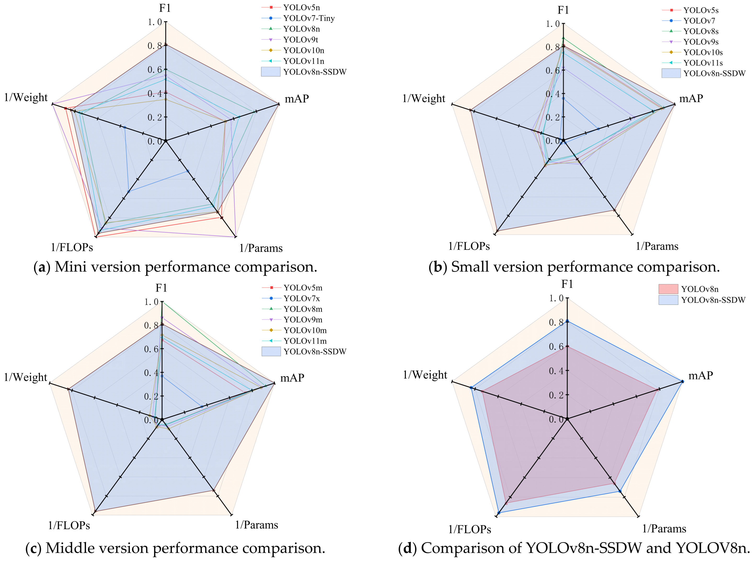
3.4. Quantitative Comparison of Various Object Detection Models

To validate this improvement, we conducted a comparative experiment under identical conditions. The results are shown in Table 3. This experiment includes several popular YOLO series object detection models, such as different variants of YOLOv5, YOLOv7, YOLOv8, YOLOv9, YOLOv10, and YOLOv11.
From the perspective of detection performance, the proposed YOLOv8n-SSDW achieves the highest mAP_50 value at 0.851, which is clearly better than other models. YOLOv8s and YOLOv8m also perform well, with mAP_50 values of 0.841 and 0.843, respectively. YOLOv11s has a mAP_50 of 0.832, but its recall rate is only 0.742. This low recall may reduce the effectiveness of target detection in real-world applications. In the YOLOv5 series, YOLOv5s has a mAP_50 of 0.840, which is better than both YOLOv5n and YOLOv5m. The overall performance of the YOLOv7 series is poor, especially for YOLOv7-Tiny, which has a mAP_50 of only 0.752. This disadvantage may be due to the model’s structure, which weakens its ability to extract features. The larger versions of YOLOv9 and YOLOv10 show relative advantages. For the F1 score, YOLOv8s and YOLOv8m have high values of 0.813 and 0.825, respectively. The proposed YOLOv8n-SSDW has an F1 score of 0.807, which is also excellent. In contrast, YOLOv7-Tiny has the lowest F1 score at only 0.730.
In terms of model lightweighting, the different YOLO series models show various characteristics. In terms of parameter count, YOLOv9t has the fewest parameters at 2.01M, making its structure the most streamlined. YOLOv5n follows with 2.51M parameters. Our proposed YOLOv8n-SSDW has a parameter count of 2.69M, which is a slight increase. At the same time, YOLOv7x has a high parameter count of 70.8 million. This indicates that it has a more complex model structure. YOLOv5n leads in computational complexity with a value of 7.1G. This means it has the highest computational efficiency. YOLOv8n-SSDW has a complexity of 7.4G, and YOLOv11n has 7.6G. In contrast, YOLOv7x reaches 188.0G. The complexity means it requires a lot of computational resources for practical use. YOLOv9t is the smallest model in terms of size, weighing just 4.7 MB. YOLOv5n is slightly larger at 5.3 MB, while YOLOv8n-SSDW is 5.6 MB. In contrast, YOLOv7x has a size of 142.1 MB, which demands more storage resources. The newer models, YOLOv10 and YOLOv11, have advantages in lightweighting while maintaining high detection performance compared to earlier versions.
In general, different YOLO series models show clear differences in performance and resource needs. YOLOv8n-SSDW is the best choice among all the models because of its outstanding overall performance.

3.5. Qualitative Comparison of Various Object Detection Models

To visually compare the overall performance of different YOLO series object detection models, we conducted a set of qualitative comparison tests. The outcomes are displayed in Figure 9a–d each display a radar chart. In these charts, each vertex represents a different performance metric. The specific metrics include the F1 score, which assesses the equilibrium between recall and precision. They also include mAP, or mean average precision at 50, which assesses the model’s detection accuracy. We also have 1/Params, which is the inverse of the number of parameters and shows the model’s lightweighting. A higher value indicates fewer parameters. We also have 1/FLOPs, which represents the inverse of the number of floating-point operations. This variable reflects the consumption of computational resources, where a higher value means less computation is needed. Lastly, we consider 1/Weight, which is inversely related to the model’s weights. This indicator reflects the storage space used, where a smaller value is better. The different colors of the lines in the charts represent different models. All metric values represent normalized results. The size of the area formed by the lines reflects the overall performance of the models across these metrics. A larger area indicates better overall performance for that model.
When we compare the mini versions of the models, such as the n or tiny versions shown in Figure 9a, we find that they perform impressively in lightweighting. However, they do not perform well in detection accuracy. Among these models, YOLOv9t shows the most significant lightweight advantage. Its values for 1/Params and 1/Weight are noteworthy, but its F1 score and mAP are lacking. As a result, its overall performance is lower than that of YOLOv8n-SSDW. Next, we look at the small versions of the models, such as the s versions shown in Figure 9b. We see an improvement in detection accuracy, but these models do not have advantages in lightweighting. Their overall performance is not satisfactory. Then, we compare the medium versions of the models, such as the m or x versions shown in Figure 9c. We observe that these models have a slight improvement in detection accuracy. However, their lightweighting performance worsens, leading to lower overall performance. Finally, when we compare YOLOv8n to YOLOv8n-SSDW, as shown in Figure 9d, we see that their performance is relatively balanced across different metrics. However, YOLOv8n is slightly weaker in some indicators compared to YOLOv8n-SSDW. The overall area it encloses is smaller, which reflects that its overall performance is inferior.
In summary, the YOLOv8n-SSDW proposed in this study shows the best overall performance. It performs impressively in both detection accuracy and model lightweighting. This study demonstrates its potential for use in detecting barnyard grass in rice fields.

3.6. Evaluation of Detection Outcomes

Figure 10 displays the results of identifying barnyard grass images in rice fields using the YOLOv8n model and the new YOLOv8n-SSDW model. The images present various complex situations. They include brightness differences in different lighting conditions, which may affect the overall visual quality. They also contain barnyard grass targets of different sizes, which can increase the difficulty of detection. The barnyard grass appears randomly between rice crops and has no specific distribution. There are also cases of obstruction and overlapping grass. The images are arranged in three rows. The first row is labeled “Original image”. It shows five unprocessed images of barnyard grass in rice fields. In these images, you can see neatly arranged rice crops and the barnyard grass that may be present among them. The second row is labeled “YOLOv8n”. This row presents the target detection outcomes using the YOLOv8n model on the corresponding original images. Detected targets and their names are highlighted in blue boxes and text. The model’s accuracy in identifying barnyard grass is illustrated in this visual representation. Errors made by the model during detection are denoted by pink boxes. The “YOLOv8n-SSDW” row showcases the detection outcomes using the YOLOv8n-SSDW model, which also highlights barnyard grass targets with blue boxes and text. A comparison of the detection performance between the two models can be observed by examining the three rows of images. This evaluation encompasses successful detection rates and the accuracy of target localization. Figure 10a–e are assigned to different image numbers to differentiate the detection outcomes of distinct groups.
Discrepancies in missed and false detections between YOLOv8n and YOLOv8n-SSDW are evident in the comparison of images. In Figure 10a, the missed detection by YOLOv8n could be attributed to the diminutive size of the barnyard grass targets. Their similarity to the surrounding crops might cause the model to struggle in distinguishing the targets from the background. In Figure 10b, YOLOv8n misses some detections. This could be because the barnyard grass is in a darker area, making it challenging for the model to capture the target’s features accurately. In Figure 10c, the missed detection might happen because the barnyard grass is somewhat hidden among the rice plants. This partial obstruction can interfere with the detection process of the model. In Figure 10d, YOLOv8n faces missed detections due to overlapping targets. The model may have trouble distinguishing between the different targets in this case. In Figure 10e, YOLOv8n shows a false detection issue. This problem may occur because similar-looking leaves mislead the model, leading to duplicate detections. In contrast, YOLOv8n-SSDW performs much better in these complex situations. This model can identify barnyard grass targets more accurately, showing greater robustness and detection accuracy.

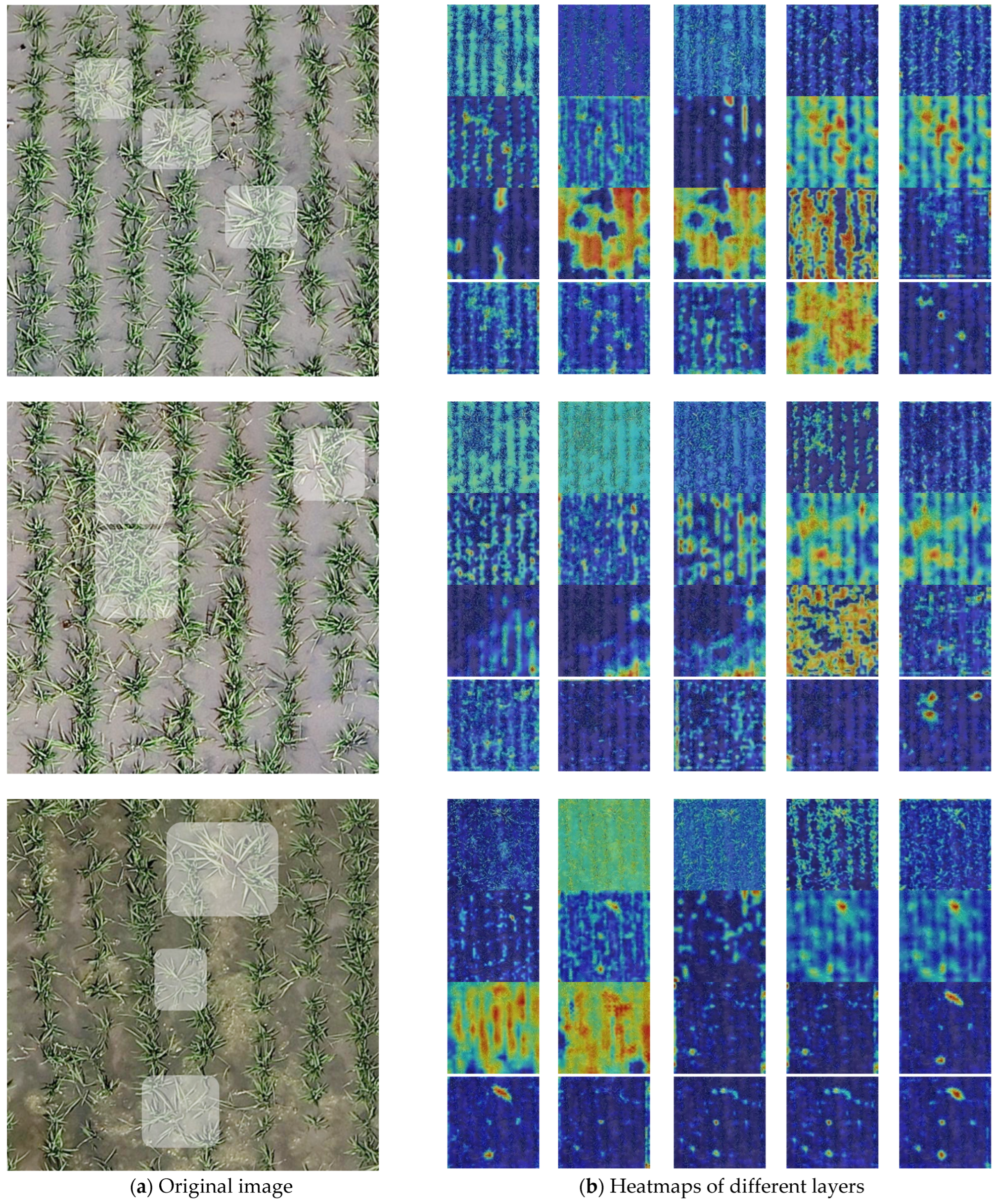
3.7. Heatmap Analysis of Different Detection Layers

The heatmap visualizes the model’s attention to different regions of the image through color intensity, where brighter colors (e.g., yellow) indicate higher attention, and darker colors (e.g., blue) represent lower attention. By comparing the original image with the heatmap, one can intuitively understand the model’s focus on targets across different layers, aiding in the analysis of feature extraction and target detection mechanisms. Figure 11 consists of two main parts: the original field image during testing and the heatmaps of different layers generated by the YOLOv8n-SSDW model when detecting this image. The left panel (a), labeled “Original image”, displays a paddy field with neatly arranged green plants, likely rice or barnyard grass. The right panel (b), labeled “Heatmaps of different layers”, presents multiple heatmaps from various layers.
In the original image, the plants exhibit a certain regularity, representing crop rows of rice in the field. Among them, plants with slight variations in size and morphology, including rice and barnyard grass, are present. This complex vegetation distribution in the field poses challenges for target detection models, as similarities in appearance, dense arrangements, and natural lighting variations may interfere with accurate target identification. From a holistic perspective, the image contains areas of brightness and darkness caused by natural lighting, which may affect the color and contrast of targets, thereby influencing the model’s visual feature-based detection performance.
The heatmaps illustrate the attention levels of the YOLOv8n-SSDW model across different layers. The results demonstrate that the proposed algorithm effectively focuses on regions containing barnyard grass. Shallower heatmaps (from left to right and top to bottom, the layers progressively deepen) tend to emphasize local details, such as leaf shapes and textures, with relatively dispersed and fine-grained color distributions, reflecting the extraction of basic visual features. In contrast, deeper heatmaps show more concentrated color distributions around specific barnyard grass targets, indicating that as the network layers deepen, the model integrates shallow features and gradually shifts focus toward holistic target recognition and localization, prioritizing positional and categorical information of barnyard grass. In some heatmaps, distinct yellow-highlighted regions are clearly concentrated on specific plants, suggesting that the YOLOv8n-SSDW model successfully captures key features of target barnyard grass at these layers, directing attention accordingly for accurate detection. However, certain heatmaps exhibit dispersed highlights or incomplete coverage of targets, possibly due to the model’s attention to background features in some layers.

3.8. Field Counting Test

Figure 12 illustrates the weed counting test conducted in a field using a drone. This section aims to validate the predictive efficiency of the proposed YOLOv8n-SSDW method through online detection tests deployed in a complex field environment. The actual field conditions present numerous interfering factors, such as background noise and uneven lighting. The principle and process of the drone weed counting test are depicted in Figure 12. The drone is equipped with a camera that captures real-time images of the field. It utilizes wireless equipment to transmit relevant information to a ground computer, which assists in processing the results. The drone primarily carries a lens, an image processor, communication devices, and a power supply, with detailed specifications of each component listed in Table 4.
The drone’s flight speed was set at 2 m per second, with a continuous forward-flight duration of 3 min, covering an approximate distance of 360 m. Manual counting revealed that the number of barnyard grasses was 643, with an average detection accuracy of 85.9%, while the average detection accuracy from laboratory tests was 86.7%. The decrease in average detection accuracy may be attributed to vibrations during the drone’s flight and interference from complex airflow in the field affecting image capture. In this field test, the average detection time for a single image was 0.05 s. Overall, the results were largely in line with expectations, indicating that the YOLOv8n-SSDW model demonstrates reliable feasibility in handling the complexities of actual rice paddy environments. Although the detection accuracy declined, it also provides a clear direction for subsequent optimization.

4. Discussion

The YOLOv8n-SSDW model proposed in this research offers advantages over existing YOLO models for barnyard grass detection in rice fields. It demonstrates enhancements in various metrics, such as F1 score, mAP, parameters, and FLOPs, compared to the original YOLOv8n model. Through the ablation study, the improved modules each contributed uniquely to the model’s performance. The incorporation of the WIoU loss function notably improved the model’s precision and mAP, consistent with prior findings by Wang et al., highlighting the effectiveness of adaptive weighting mechanisms in optimizing bounding box regression outcomes [35]. Additionally, the SEAM attention mechanism improved the model’s ability to focus on barnyard grass features amidst complex backgrounds. Similar attention mechanisms have been shown to enhance model performance effectively in other studies on plant disease detection [36]. The SRCConv module, featuring a unique design for coordinate convolution and incorporating residual connections, maintains high detection accuracy despite its lightweight nature. This finding aligns with Hu and colleagues’ assertion that separable convolutions and residual connections can improve model efficiency and stability [37].
However, the model still exhibits certain limitations. Decreasing model parameters results in lower recognition accuracy, despite optimization in the SRCConv module, suggesting potential for enhancement. Under complex field conditions, such as extreme weather events involving strong winds or dust storms that severely degrade image quality, the model’s detection accuracy and robustness are significantly compromised. This observation aligns with the findings by Chen et al. regarding the sensitivity of deep learning models to environmental variations [38]. Additionally, while the model performs well on the dataset constructed in this study, its generalization capability across different regions and rice varieties requires further validation. Factors such as varying soil colors, rice planting densities, and weed species distributions may influence model performance [39].
To address these challenges, future research could focus on the following directions. First, further optimization of lightweight convolutional modules could be pursued by exploring more efficient architectural designs that minimize parameter counts while preserving feature information, potentially drawing inspiration from novel lightweight network structures [40]. Second, to enhance the model’s adaptability to complex environments, training datasets could be augmented with images captured under various extreme conditions, enabling the model to learn more diverse features and improve robustness [41]. Concurrently, field tests across multiple regions and rice varieties could be conducted to collect more heterogeneous data for model refinement and enhanced generalization.
Moreover, integrating the proposed model with other advanced technologies presents a promising research avenue. For instance, improvements in UAV flight control systems or the development of anti-vibration imaging techniques could mitigate the impact of flight-induced vibrations on image quality. Alternatively, combining spectral feature-based weed detection methods with the current model [42] may leverage unique spectral signatures to improve accuracy, particularly in distinguishing morphologically similar weeds. The integration of the model with IoT technologies could also enable real-time, remote monitoring and management of field weeds, thereby advancing smart agricultural practices [43]. In summary, the YOLOv8n-SSDW model proposed in this study offers a novel solution for barnyard grass detection in paddy fields, yet continuous refinement is necessary to better meet the practical demands of agricultural production.

5. Conclusions

In response to the prevalent issues of insufficient accuracy, large parameter counts, and high computational complexity in existing weed detection models, this study constructed a barnyard grass detection dataset and proposed a lightweight field barnyard grass detection model—YOLOv8n-SSDW. A novel SRCConv was designed to replace the convolution modules of the original model. By incorporating coordinate details into the convolution process, this design improves the model’s target localization capabilities. The utilization of separable convolutions decreases computational complexity and incorporates residual connections to enhance feature propagation. This approach ensures the stability of barnyard grass feature extraction in complex backgrounds, maintaining recognition accuracy while lowering computational costs, thereby making the model more lightweight and efficient. The sensitivity of the model to edge detail features of barnyard grass was enhanced by introducing the SEAM attention mechanism and upgrading the global average pooling layer to a global max pooling layer. Moreover, a lightweight and efficient upsampling module, Dysample, was incorporated to enhance the resolution of feature maps. The loss function for the training model was redefined as WIoU to improve the classification and regression accuracy of detection boxes. The efficacy of the model was confirmed through various experimental cohorts. The mAP_50 of the YOLOv8n-SSDW model reached 0.851, with a parameter count of 2.69M and FLOPs of 7.4G, resulting in an 11.1% reduction in model size to only 5.6 MB. YOLOv8n-SSDW outperformed the baseline model, exhibiting a higher accuracy, recall rate, and mAP, along with reduced loss values. When compared to other state-of-the-art models in the YOLO series, YOLOv8n-SSDW exhibited the highest overall performance. On-site tests conducted by combining drones with ground-based computers and using the YOLOv8n-SSDW model show that due to vibration and airflow, the accuracy slightly decreased. However, the overall performance met standards, preliminarily verifying its feasibility for barnyard grass detection in complex rice field scenarios. Future research could further optimize the model structure or enhance the shock resistance of drone image acquisition to improve the adaptability in complex environments, thereby promoting the continuous development of weed detection technology in rice paddies to better serve agricultural production practices.

Author Contributions

Conceptualization, Y.S.; data curation, H.G., X.C. and M.L.; formal analysis, Y.S. and Y.C.; investigation, H.G., X.C. and M.L.; methodology, Y.S.; resources, Y.C.; software, Y.S.; supervision, Y.S.; validation, Y.C.; visualization, Y.S.; writing—original draft, Y.S.; writing—review and editing, Y.C. and B.F. All authors have read and agreed to the published version of the manuscript.

Funding

This research was funded by the Key Research Project of the Liaoning Provincial Department of Education (JYTZD2023123).

Data Availability Statement

The data presented in this study can be requested from the corresponding author. The data are not currently available for public access because they are part of an ongoing research project.

Acknowledgments

The authors would like to thank the anonymous reviewers for their critical comments and suggestions for improving the manuscript.

Conflicts of Interest

The authors declare no conflicts of interest.

References

  1. Alagbo, O.O.; Akinyemiju, O.A.; Chauhan, B.S. Weed Management in Rainfed Upland Rice Fields under Varied Agro-Ecologies in Nigeria. Rice Sci. 2022, 29, 328–339. [Google Scholar] [CrossRef]
  2. Yuan, Q.; Tian, Z.; Lv, W.; Huang, W.; Sun, X.; Lv, W.; Bi, Y.; Shen, G.; Zhou, W. Effects of common rice field weeds on the survival, feeding rate and feeding behaviour of the crayfish Procambarus clarkii. Sci. Rep. 2021, 11, 19327. [Google Scholar] [CrossRef]
  3. Singh, M.; Bhullar, M.S.; Gill, G. Integrated weed management in dry-seeded rice using stale seedbeds and post sowing herbicides. Field Crops Res. 2018, 224, 182–191. [Google Scholar] [CrossRef]
  4. Feng, T.; Sun, W.; Wang, J.; Lei, T.; Wang, L.; Xie, Y.; Zhou, H.; Zhu, F.; Ma, H. Susceptibility monitoring and metabolic resistance study of Echinochloa crus-galli to three common herbicides in rice regions of the Mid-Lower Yangtze, China. Crop Prot. 2025, 191, 107108. [Google Scholar] [CrossRef]
  5. Dass, A.; Shekhawat, K.; Choudhary, A.K.; Sepat, S.; Rathore, S.S.; Mahajan, G.; Chauhan, B.S. Weed management in rice using crop competition-a review. Crop Prot. 2017, 95, 45–52. [Google Scholar] [CrossRef]
  6. Zhang, Z.; Li, R.; Zhao, C.; Qiang, S. Reduction in weed infestation through integrated depletion of the weed seed bank in a rice-wheat cropping system. Agron. Sustain. Dev. 2021, 41, 10. [Google Scholar] [CrossRef]
  7. Ju, J.; Chen, G.; Lv, Z.; Zhao, M.; Sun, L.; Wang, Z.; Wang, J. Design and experiment of an adaptive cruise weeding robot for paddy fields based on improved YOLOv5. Comput. Electron. Agric. 2024, 219, 108824. [Google Scholar] [CrossRef]
  8. Hadayat, A.; Zahir, Z.A.; Cai, P.; Gao, C. Integrated application of synthetic community reduces consumption of herbicide in field Phalaris minor control. Soil Ecol. Lett. 2024, 6, 230207. [Google Scholar] [CrossRef]
  9. Rai, N.; Zhang, Y.; Ram, B.G.; Schumacher, L.; Yellavajjala, R.K.; Bajwa, S.; Sun, X. Applications of deep learning in precision weed management: A review. Comput. Electron. Agric. 2023, 206, 107698. [Google Scholar] [CrossRef]
  10. Sun, Y.; Li, M.; Liu, M.; Zhang, J.; Cao, Y.; Ao, X. A statistical method for high-throughput emergence rate calculation for soybean breeding plots based on field phenotypic characteristics. Plant Methods 2025, 21, 40. [Google Scholar] [CrossRef]
  11. Ur Rehman, M.; Eesaar, H.; Abbas, Z.; Seneviratne, L.; Hussain, I.; Chong, K.T. Advanced drone-based weed detection using feature-enriched deep learning approach. Knowl. Based Syst. 2024, 305, 112655. [Google Scholar] [CrossRef]
  12. Ren, S.; He, K.; Girshick, R.; Sun, J. Faster R-CNN: Towards real-time object detection with region proposal networks. IEEE Trans. Pattern Anal. Mach. Intell. 2017, 39, 1137–1149. [Google Scholar] [CrossRef]
  13. Redmon, J.; Farhadi, A. YOLO9000: Better, faster, stronger. arXiv 2016, arXiv:1612.08242. [Google Scholar]
  14. Redmon, J.; Divvala, S.; Girshick, R.; Farhadi, A. You only look once: Unified, real-time object detection. In Proceedings of the IEEE Conference on Computer Vision and Pattern Recognition, Las Vegas, NV, USA, 27–30 June 2016; IEEE: Piscataway, NJ, USA, 2016; pp. 779–788. [Google Scholar]
  15. Varghese, R.; Sambath, M. YOLOv8: A novel object detection algorithm with enhanced performance and robustness. In Proceedings of the International Conference on Advances in Data Engineering and Intelligent Computing Systems, Chennai, India, 18–19 April 2024; IEEE: Piscataway, NJ, USA, 2024; pp. 1–6. [Google Scholar] [CrossRef]
  16. Guo, Z.; Cai, D.; Zhou, Y.; Xu, T.; Yu, F. Identifying rice field weeds from unmanned aerial vehicle remote sensing imagery using deep learning. Plant Methods 2024, 20, 105. [Google Scholar] [CrossRef]
  17. Farooq, U.; Rehman, A.; Khanam, T.; Amtullah, A.; Bou-rabee, M.A.; Tariq, M. Lightweight deep learning model for weed detection for IoT devices. In Proceedings of the 2022 2nd International Conference on Emerging Frontiers in Electrical and Electronic Technologies, Patna, India, 24–25 June 2022; IEEE: Piscataway, NJ, USA, 2022; pp. 1–6. [Google Scholar]
  18. Prasad, D. Real-time weed detection and classification using deep learning models and IoT-based edge computing for social learning applications. In Augmented and Virtual Reality in Social Learning: Technological Impacts and Challenges; De Gruyter: Berlin, Germany; Boston, MA, USA, 2024; pp. 241–268. [Google Scholar] [CrossRef]
  19. Ma, C.; Chi, G.; Ju, X.; Zhang, J.; Yan, C. YOLO-CWD: A novel model for crop and weed detection based on improved YOLOv8. Crop Prot. 2025, 192, 107169. [Google Scholar] [CrossRef]
  20. Tang, B.; Zhou, J.; Pan, Y.; Qu, X.; Cui, Y.; Liu, C.; Li, X.; Zhao, C.; Gu, X. Recognition of maize seedling under weed disturbance using improved YOLOv5 algorithm. Measurement 2025, 242 Pt B, 115938. [Google Scholar] [CrossRef]
  21. Fan, X.; Sun, T.; Chai, X.; Zhou, J. YOLO-WDNet: A lightweight and accurate model for weeds detection in cotton field. Comput. Electron. Agric. 2024, 225, 109317. [Google Scholar] [CrossRef]
  22. Saleem, M.H.; Potgieter, J.; Arif, K.M. Weed Detection by Faster RCNN Model: An Enhanced Anchor Box Approach. Agronomy 2022, 12, 1580. [Google Scholar] [CrossRef]
  23. Peng, H.; Li, Z.; Zhou, Z.; Shao, Y. Weed detection in paddy field using an improved RetinaNet network. Comput. Electron. Agric. 2022, 199, 107179. [Google Scholar] [CrossRef]
  24. Liu, T.; Zhao, Y.; Wang, H.; Wu, W.; Yang, T.; Zhang, W.; Zhu, S.; Sun, C.; Yao, Z. Harnessing UAVs and deep learning for accurate grass weed detection in wheat fields: A study on biomass and yield implications. Plant Methods 2024, 20, 144. [Google Scholar] [CrossRef]
  25. Chen, H.; Zhang, Y.; He, C.; Chen, C.; Zhang, Y.; Chen, Z.; Jiang, Y.; Lin, C.; Ma, R.; Qi, L. PIS-Net: Efficient weakly supervised instance segmentation network based on annotated points for rice field weed identification. Smart Agric. Technol. 2024, 9, 100557. [Google Scholar] [CrossRef]
  26. Dang, F.; Chen, D.; Lu, Y.; Li, Z. YOLOWeeds: A novel benchmark of YOLO object detectors for multi-class weed detection in cotton production systems. Comput. Electron. Agric. 2023, 205, 107655. [Google Scholar] [CrossRef]
  27. Liu, R.; Lehman, J.; Molino, P.; Petroski Such, F.; Frank, E.; Sergeev, A.; Yosinski, J. An intriguing failing of convolutional neural networks and the CoordConv solution. arXiv 2018, arXiv:1807.03247. [Google Scholar]
  28. Wang, Y.; Zhang, J.; Kan, M.; Shan, S.; Chen, X. Self-supervised equivariant attention mechanism for weakly supervised semantic segmentation. In Proceedings of the IEEE/CVF Conference on Computer Vision and Pattern Recognition, Seattle, WA, USA, 13–19 June 2020; IEEE: Piscataway, NJ, USA, 2020; pp. 12235–12244. [Google Scholar] [CrossRef]
  29. Liu, W.; Lu, H.; Fu, H.; Cao, Z. Learning to upsample by learning to sample. In Proceedings of the IEEE/CVF International Conference on Computer Vision, Paris, France, 1–6 October 2023; IEEE: Piscataway, NJ, USA, 2023; pp. 6004–6014. [Google Scholar] [CrossRef]
  30. Zheng, Z.; Wang, P.; Liu, W.; Li, J. Enhancing geometric factors in model learning and inference for object detection and instance segmentation. IEEE Access 2022, 52, 8574–8586. [Google Scholar] [CrossRef]
  31. Du, S.; Zhang, B.; Zhang, P. Scale-Sensitive IoU Loss: An Improved Regression Loss Function in Remote Sensing Object Detection. IEEE Access 2021, 9, 141258–141272. [Google Scholar] [CrossRef]
  32. Jin, S.; Cao, Q.; Li, J.; Wang, X.; Li, J.; Feng, S.; Xu, T. Study on lightweight rice blast detection method based on improved YOLOv8. Pest Manag. Sci. 2025. [Google Scholar] [CrossRef]
  33. Tong, Z.; Chen, Y.; Xu, Z.; Yu, R. Wise-IoU: Bounding Box Regression Loss with Dynamic Focusing Mechanism. arXiv 2023, arXiv:2301.10051. [Google Scholar] [CrossRef]
  34. San, K.H.; Kondo, T.; Maruka Tat, S.; Hara-Azumi, Y. A Comparative Study of Loss Functions for Arbitrary-Oriented Object Detection in Aerial Images. In Proceedings of the 2024 21st International Joint Conference on Computer Science and Software Engineering (JCSSE), Phuket, Thailand, 19–22 June 2024; IEEE: Piscataway, NJ, USA, 2024; pp. 1–8. [Google Scholar] [CrossRef]
  35. Wang, J.; Tan, D.; Sui, L.; Guo, J.; Wang, R. Wolfberry recognition and picking-point localization technology in natural environments based on improved Yolov8n-Pose-LBD. Comput. Electron. Agric. 2024, 227 Pt 1, 109551. [Google Scholar] [CrossRef]
  36. Alirezazadeh, P.; Schirrmann, M.; Stolzenburg, F. Improving Deep Learning-based Plant Disease Classification with Attention Mechanism. Gesunde Pflanz. 2023, 75, 49–59. [Google Scholar] [CrossRef]
  37. Hu, Y.; Huang, Y.; Zhang, K. Multi-scale information distillation network for efficient image super-resolution. Knowl. Based Syst. 2023, 275, 110718. [Google Scholar] [CrossRef]
  38. Chen, Z.; Liu, H.; Xu, C.; Wu, X.C.; Liang, B.; Cao, J.; Chen, D. Modeling vegetation greenness and its climate sensitivity with deep-learning technology. Ecol. Evol. 2021, 11, 7335–7345. [Google Scholar] [CrossRef] [PubMed]
  39. Xia, X.; Wang, M.; Shi, Y.; Huang, Z.; Liu, J.; Men, H.; Fang, H. Identification of white degradable and non-degradable plastics in food field: A dynamic residual network coupled with hyperspectral technology. Spectrochim. Acta Part A Mol. Biomol. Spectrosc. 2023, 296, 122686. [Google Scholar] [CrossRef] [PubMed]
  40. Ouyang, M.; Chen, Z. JPEG Quantized Coefficient Recovery via DCT Domain Spatial-Frequential Transformer. IEEE Trans. Image Process. 2024, 33, 3385–3398. [Google Scholar] [CrossRef] [PubMed]
  41. Lee, H.; Kang, S.; Chung, K. Robust Data Augmentation Generative Adversarial Network for Object Detection. Sensors 2023, 23, 157. [Google Scholar] [CrossRef]
  42. Zhang, Y.; Gao, J.; Cen, H.; Lu, Y.; Yu, X.; He, Y.; Pieters, J.G. Automated spectral feature extraction from hyperspectral images to differentiate weedy rice and barnyard grass from a rice crop. Comput. Electron. Agric. 2019, 159, 42–49. [Google Scholar] [CrossRef]
  43. Boursianis, A.D.; Papadopoulou, M.S.; Diamantoulakis, P.; Liopa-Tsakalidi, A.; Barouchas, P.; Salahas, G.; Karagiannidis, G.; Wan, S.; Goudos, S.K. Internet of Things (IoT) and Agricultural Unmanned Aerial Vehicles (UAVs) in smart farming: A comprehensive review. Internet Things 2022, 18, 100187. [Google Scholar] [CrossRef]
Figure 1. Effect of data augmentation on images.
Agriculture 15 01510 g001
Figure 2. Structural diagram of YOLOv8n-SSDW.
Agriculture 15 01510 g002
Figure 3. Structural diagram of SRCConv.
Agriculture 15 01510 g003
Figure 4. Structural diagram of SEAM.
Agriculture 15 01510 g004
Figure 5. Structural diagram of DySample.
Agriculture 15 01510 g005
Figure 6. The principle of IoU loss in boundary box regression.
Agriculture 15 01510 g006
Figure 7. P, R curves and mAP curves for YOLOv8n and YOLOv8n-SSDW.
Agriculture 15 01510 g007
Figure 8. Loss curves for YOLOv8n and YOLOv8n-SSDW.
Agriculture 15 01510 g008
Figure 9. Radar charts comparing the performance of different YOLO series object detection models.
Agriculture 15 01510 g009
Figure 10. Detection results of barnyard grass using YOLOv8n and YOLOv8n-SSDW.
Agriculture 15 01510 g010
Figure 11. Heatmaps of different detection layers of YOLOv8n-SSDW alongside the original image.
Agriculture 15 01510 g011
Figure 12. Drone-based field weed counting test.
Agriculture 15 01510 g012
Table 1. Comparison of detection performance of YOLO series models.
Baseline ModelPrecisionRecallF1mAP_50Parameters (M)FLOPs (G)Model Size (MB) Inference Time (ms)
YOLOv5n0.7690.7690.7690.8042.517.15.314.6
YOLOv7-Tiny0.7520.7090.7300.7526.0113.012.312.7
YOLOv8n0.8290.7490.7870.8293.018.26.313.6
YOLOv9-Tiny0.8060.7600.7820.8092.017.84.737.2
YOLOv10n0.7810.7450.7630.8042.708.35.818.7
YOLOv11n0.8030.7560.7790.8162.917.66.115.4
Table 2. Ablation study results.
Baseline ModelPRmAP_50Params (M)FLOPs (G)Weight (MB)
YOLOv8n0.8290.7490.8293.018.26.3
YOLOv8n-Dysample0.8260.7480.8343.028.26.3
YOLOv8n-Dysample-WIoU0.8730.7600.8413.028.26.3
YOLOv8n-Dysample-WIoU-SRCConv0.8720.7670.8372.587.25.4
YOLOv8n-Dysample-WIoU-SRCConv-SEAM0.8670.7550.8512.697.45.6
Table 3. Results of the comparison among different models.
ModelPrecisionRecallF1mAP_50Parameters (M)FLOPs (G)Model Size (MB) Infer Time (ms)
YOLOv5n0.7690.7690.7690.8042.517.15.314.6
YOLOv5s0.8240.7910.8070.8409.1224.018.515.6
YOLOv5m0.8170.7730.7940.82525.164.250.517.1
YOLOv7-Tiny0.7520.7090.7300.7526.0113.012.312.7
YOLOv70.7710.7570.7640.78336.5103.274.814.5
YOLOv7x0.830.7090.7650.78770.8188.0142.117.5
YOLOv8n0.8290.7490.7870.8293.018.26.313.6
YOLOv8s0.8410.7860.8130.84111.128.622.514.8
YOLOv8m0.8610.7910.8250.84325.979.052.017.6
YOLOv9t0.8060.7600.7820.8092.017.84.737.2
YOLOv9s0.8230.7570.7890.8157.2927.415.339.6
YOLOv9m0.8410.7840.8120.84020.277.540.941.3
YOLOv10n0.7810.7450.7630.8042.708.35.818.7
YOLOv10s0.8490.7680.8060.8398.0524.616.519.1
YOLOv10m0.8330.7650.7980.83916.563.833.521.8
YOLOv11n0.8030.7560.7790.8162.917.66.115.4
YOLOv11s0.8690.7420.8010.83210.726.521.816.9
YOLOv11m0.8190.7750.7960.83123.985.448.118.5
YOLOv8n-SSDW0.8670.7550.8070.8512.697.45.615.3
Table 4. Main payload equipment of the UAV.
DevicesRelated Description
Camera lens Zenmuse P1 lens for field barnyard grass images
Image processorJetson nano B01 used to detect barnyard grass in the field
4G/5G network connection end point Based on DJI airborne SDK development, real-time transmission of collected image data to the ground
Power supplyTB60 smart flight battery for UAV power supply
Disclaimer/Publisher’s Note: The statements, opinions and data contained in all publications are solely those of the individual author(s) and contributor(s) and not of MDPI and/or the editor(s). MDPI and/or the editor(s) disclaim responsibility for any injury to people or property resulting from any ideas, methods, instructions or products referred to in the content.

