Research on SPAD Inversion of Rice Leaves at a Field Scale Based on Machine Vision and Leaf Segmentation Techniques

Abstract

Crop chlorophyll contents affect growth, and accurate assessment aids field management. SPAD (Soil Plant Analysis Development) values of leaves were mainly used to estimate chlorophyll content. Background interference affects the accuracy of SPAD value inversion. To address this issue, a rice leaf SPAD inversion method combining deep learning and feature selection is proposed. First, a leaf segmentation model based on U-Net was established. Then, the color features of leaf images were extracted. Seven color features highly correlated with SPAD were selected via the Pearson correlation coefficient and recursive feature elimination optimization. Finally, leaf SPAD inversion models based on random forest, support vector regression, BPNNs, and XGBoost were established. The results demonstrated that the U-Net could achieve accurate segmentation of leaves with a maximum mean intersection over union (MIoU) of 88.23. The coefficients of determination R² between the anticipated and observed SPAD values of the four models were 0.819, 0.829, 0.896, and 0.721, and the root mean square errors (RMSEs) were 2.223, 2.131, 1.564, and 2.906. Through comparison, the method can accurately predict SPAD in different low-definition and saturation images, showing a certain robustness. It can offer technical support for accurate, nondestructive, and expedited evaluation of crop leaves’ chlorophyll content via machine vision.

1. Introduction

The chlorophyll content of crop leaves is associated with crop photosynthesis and is strongly linked to the growth and yield of crops [1,2]. A high chlorophyll content indicates strong crop growth, adequate nutrition, and strong stress resistance [3]. Therefore, the efficient and precise quantification of the chlorophyll content in crop leaves is helpful for evaluating crop growth status and thus supports the implementation of farm crop growth management and yield increase measures [4].

The conventional approach for determining chlorophyll content involves chemical analysis. Although this technique can detect the chlorophyll content of leaves accurately, it is destructive to plants during the detection process. It is time-consuming, complex, expensive, and incapable of meeting the demand for the expeditious and nondestructive acquisition of chlorophyll content in the field [5]. With the rapid advancements in remote sensing and artificial intelligence technology, there are two main types of nondestructive monitoring technologies for chlorophyll content at present, namely, spectral analysis [6] and image processing based on machine vision [7].

Spectroscopic analysis can be employed to establish linear or nonlinear relationships between spectral characteristics and chlorophyll content and can indirectly estimate chlorophyll content. The main spectral features used in this method include multiple vegetation indices, such as the normalized difference vegetation index (NDVI) [8], ratio vegetation index (RVI) [9], soil-adjusted vegetation index (SAVI) [10], green normalized difference vegetation index (GNDVI) [11], and green ratio vegetation index (GRVI) [12]. Modeling is then carried out via methods such as regression analysis, machine learning, and deep learning. Good results have been obtained for chlorophyll inversion in cotton [13], corn [14], rice [4], and other crops. However, the price and cost of spectrometers are high, and some equipment needs to be carried out on drones to achieve efficient data acquisition; thus, the popularity of agricultural production is relatively low, it is mostly used for scientific research and production censuses, and the application scope is limited to a certain extent.

The chlorophyll content of crops is reflected not only in their spectral characteristics but also in the color features of their leaves. By applying machine vision technology to image processing, rapid, noncontact monitoring and analysis of chlorophyll content can be effectively accomplished [15]. This technology not only improves the efficiency of data collection but can also be used to evaluate the growth of crops in real time and provide timely and accurate decision support for agricultural production. By extracting the color eigenvalues of leaves, researchers have screened out parameters highly correlated with chlorophyll content and established RF [16], SVM [17], XGBoost [18], and other machine learning-based chlorophyll content estimation models. The method is usually based on color characteristic parameters of the RGB color space, such as G-R, (G-R)/(G+R), and R/(G+B), to establish positive and negative correlations with chlorophyll content [7,19]. In addition, some studies have been based on color characteristic parameters of the HSI color space [20], color characteristic parameters of the HSV color space [21], the dark green color index (DGCI) [22], and other parameters to establish correlations with chlorophyll content for chlorophyll content inversion [7]. Compared with the spectral analysis method, the image processing method based on machine vision can be used to collect images via devices such as digital cameras or smartphones, which reduces the monitoring cost and provides an efficient, economical, and practical means of monitoring chlorophyll content. With the continuous progress in machine vision technology and artificial intelligence algorithms, image processing-based chlorophyll content monitoring methods are anticipated to have broader implementation and dissemination in future agricultural production practices.

Although chlorophyll content monitoring results can be obtained quickly via machine vision-based image processing, the chlorophyll content obtained via this method is susceptible to the impact of the field environment on the image, especially the background soil or other components of the crop; therefore, the target leaf area needs to be accurately extracted before inversion of the chlorophyll content is performed. The rice leaf segmentation technique can segment the leaves of a crop to exclude interference from nontarget region images, such as spikes, stalks, and the soil background during chlorophyll inversion. Current rice image leaf segmentation techniques have been widely studied [23], mainly including conventional image segmentation methodologies and image segmentation techniques based on deep learning. Among them, traditional image segmentation techniques are usually based on different color space features [24,25] via algorithms such as thresholding [26] and clustering [27,28] segmentation of crop canopy leaves. However, this segmentation technique is sensitive to changes in lighting conditions, background complexity, and crop morphology and is susceptible to noise, resulting in inaccurate segmentation or clustering results. The rapid advancement of computer vision has led to the increasingly widespread application of deep learning-based image segmentation techniques in the field of image processing. Among them, the convolutional neural network (CNN) has been effectively applied to a wide range of machine vision tasks [29], and the method is able to better cope with variations in target morphology and complex background information by automatically extracting multilevel features from images. The U-Net [30] network is an image segmentation model based on a CNN, which is widely employed in segmentation tasks because of its smaller model size, fewer parameters, higher processing speed, and greater adaptability to address a low volume of training data [31,32]. Many studies have shown that U-Net is more effective in plant segmentation tasks [33,34], and better results have been achieved in the segmentation of crops such as figs, lettuce, and corn [35,36,37]. Therefore, the U-Net network has significant advantages in improving the accuracy of rice leaf segmentation and provides a reliable preprocessing step for accurate inversion of chlorophyll content, which is able to adaptively learn the image features and reduce the interference caused by the environment and other factors to achieve more stable and accurate monitoring of the chlorophyll content under complex field conditions. Furthermore, a strong correlation exists between the SPAD values obtained from portable chlorophyll meters and the chlorophyll content, with higher SPAD values indicating greater chlorophyll concentrations. Consequently, SPAD values are commonly used as reliable indicators for assessing actual chlorophyll content levels. [38,39].

On the basis of the above discussion, this study presents a machine vision inversion method for the SPAD of rice leaves by integrating deep learning and feature optimization in response to the shortcomings of the existing machine vision techniques in leaf SPAD inversion, which are applicable only to leaves with simple backgrounds. First, a rice leaf segmentation model was constructed on the basis of the U-Net deep learning network, which realized efficient and precise segmentation of rice leaves under complex field conditions. Then, on the basis of the segmented image of the rice leaves, two-stage feature optimization was performed by combining the PCC and the RFE methods, and the color feature parameters suitable for SPAD inversion were screened out. Finally, high-precision inversion of rice leaf SPAD values was realized via a machine learning (ML) model. The chlorophyll inversion method proposed in this study can provide technical support for accurate, nondestructive, and rapid monitoring of the chlorophyll content of crop leaves under complex backgrounds, with the goal of providing scientific support for the assessment and management of crop growth status.

2. Study Area and Data Sources

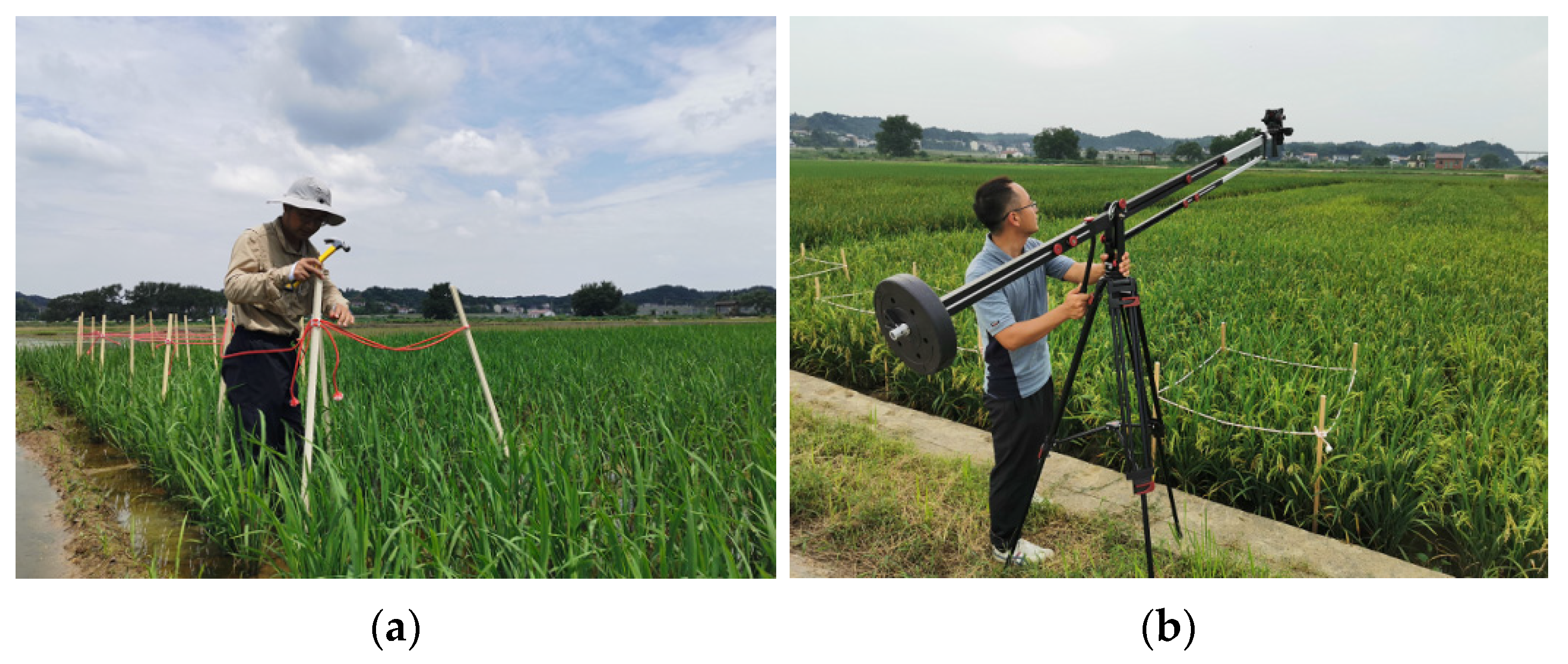
2.1. Experimental Plots and Data Collection

The experimental plots were set up in Gaoqiao Town of Changsha County, Hunan Academy of Agricultural Sciences, China. The rice used in the experiment was early rice, which included two varieties: the hybrid rice Zhongzao 39 (variety A) and the conventional rice Xiangzaoxian 24 (variety B). Each variety of rice was split into six plots, each with a size of 1 square meter. Chlorophyll formation is closely related to nitrogen supply, so to obtain a large range of chlorophyll SPAD values, each rice variety in this study was set up with six nitrogen application levels of 0, 3, 6, 9, 12, and 15 kg, with a basal-to-follow-up fertilizer ratio of 6:4, and four replications. The experimental plot layout and image acquisition are shown in Figure 1.

The data for this study were collected on 25 June 2021, 29 June 2021, 5 July 2021, 9 July 2021, and 14 July 2021. Rice images were taken vertically by a digital camera set up at a height of 2 m above the ground and repeated six times for each sample in each period, and one of the clearest images was selected for leaf SPAD content inversion. Moreover, the relative chlorophyll content of the experimental plots was measured via a SPAD_502 handheld chlorophyll meter [40]. Five points of rice sample SPAD value data were collected randomly in the experimental plot, and the main leaf veins were avoided. Three distinct locations on each leaf were selected, with three measurements taken at each location. The mean value was calculated and recorded as the SPAD value for the experimental field leaves. The experiment resulted in 60 sets of rice images as well as SPAD value data.

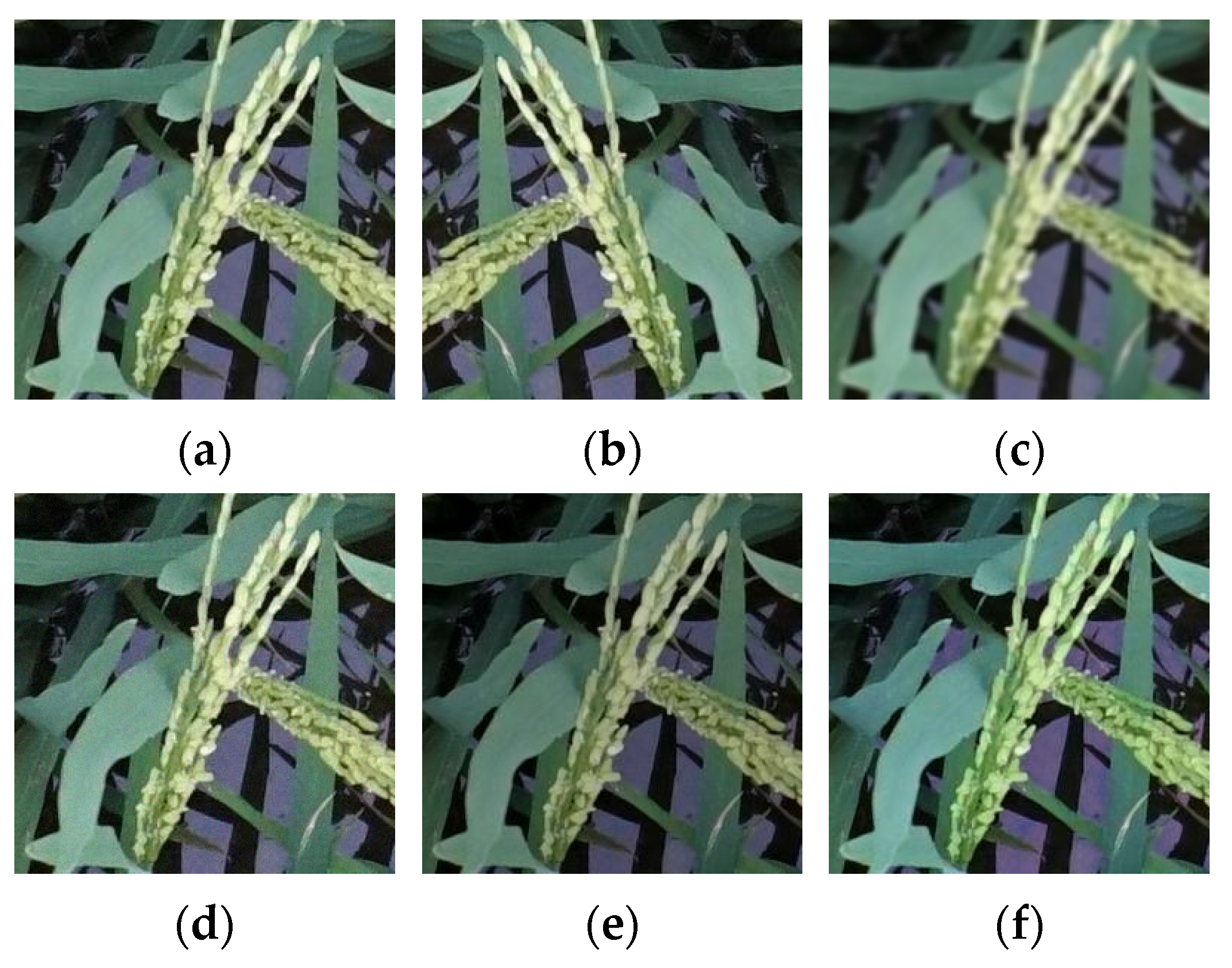
2.2. Image Segmentation Dataset

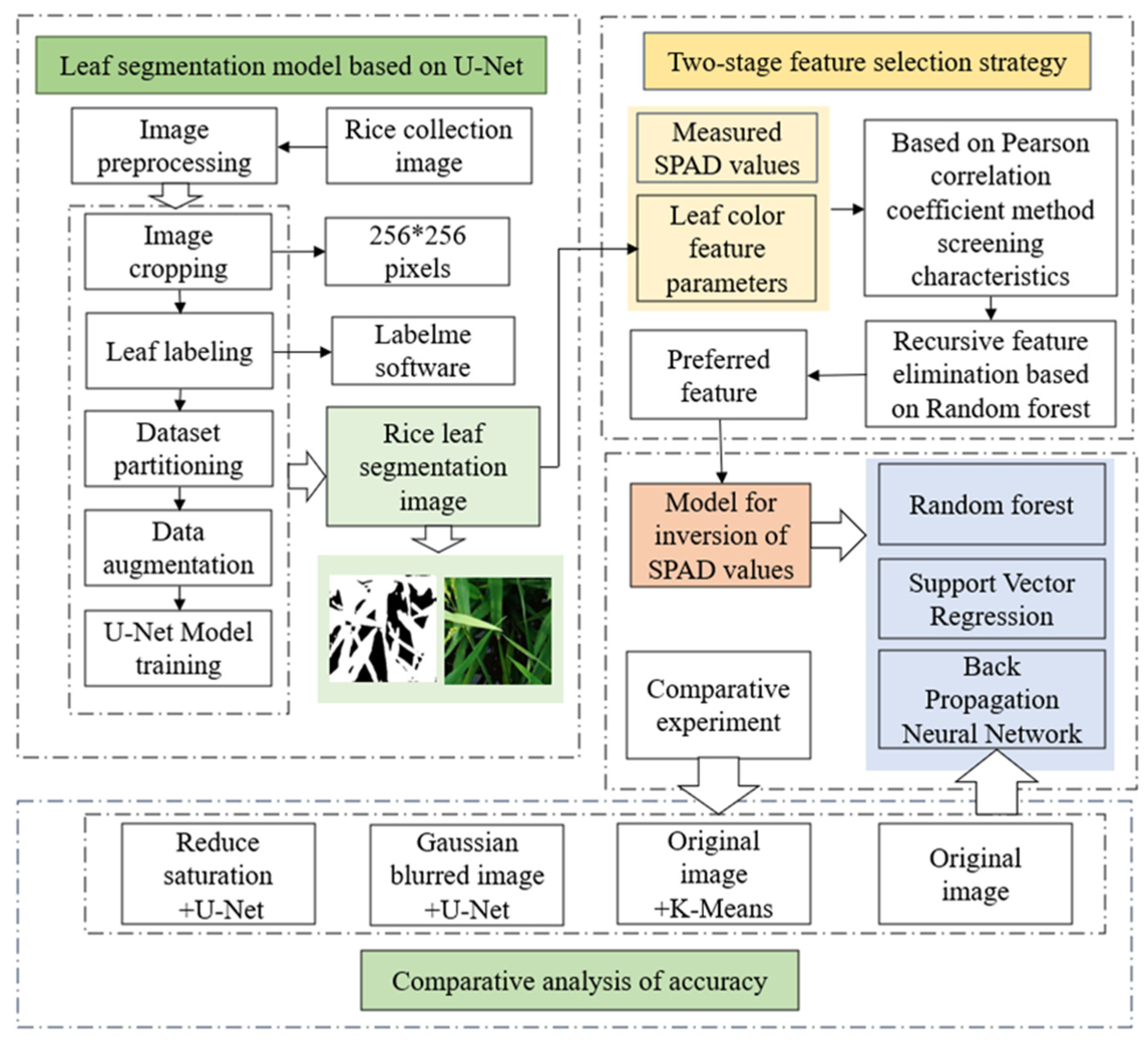
When manually annotating the original rice images, larger image sizes can lead to poor results and increased computational overhead when the model is trained. To mitigate the costs associated with data processing annotation and reduce the model’s training duration, the captured images are uniformly cropped to a pixel size of 256 × 256. Labelme annotation software (version number 5.5.0) was used for the annotation of the rice leaves, which were randomly partitioned into training and validation sets at a ratio of 7:3. To obtain more training samples, the robustness of the segmentation model and the ability to generalize image enhancement were enhanced. The main processing methods include mirroring, Gaussian noise, blurring, and other methods, and the enhancement of the sample graph is shown in Figure 2. The dataset after image enhancement includes 1760 leaf images, of which the training and validation sets include 1232 and 528 images, respectively.

3. Method

In this study, we propose a rice leaf SPAD machine vision inversion method that incorporates deep learning and feature optimization in response to the shortcomings of the existing machine vision techniques in leaf SPAD inversion, which are applicable only to leaves with simple backgrounds. First, to construct the rice leaf dataset, the U-Net network with a jump connection structure was used as the segmentation model to achieve efficient and precise segmentation of rice leaves in a complex field background. Then, to extract the leaf color feature values, we combined the Pearson correlation coefficient method and the RFE method to carry out two-stage feature optimization and screened out the color feature parameters suitable for SPAD inversion. Finally, the establishment of a SPAD inversion model for rice leaves on the basis of the ML framework enabled the accurate estimation of SPAD values in rice leaves. Figure 3 illustrates the technical roadmap of this research.

3.1. Rice Leaf Segmentation Model Based on the U-Net Architecture

The rice leaf segmentation technique can effectively separate the leaf portion from the rice spike and background soil or other components of the crop, providing background interference-free leaf images for subsequent leaf SPAD inversion model construction. In segmentation modeling, the U-Net network is able to extract key characteristics effectively from an image and preserve important details while restoring spatial resolution because of its unique encoder–decoder structure [35]. Therefore, this study realizes accurate segmentation of leaves on the basis of the constructed rice leaf dataset and U-Net network.

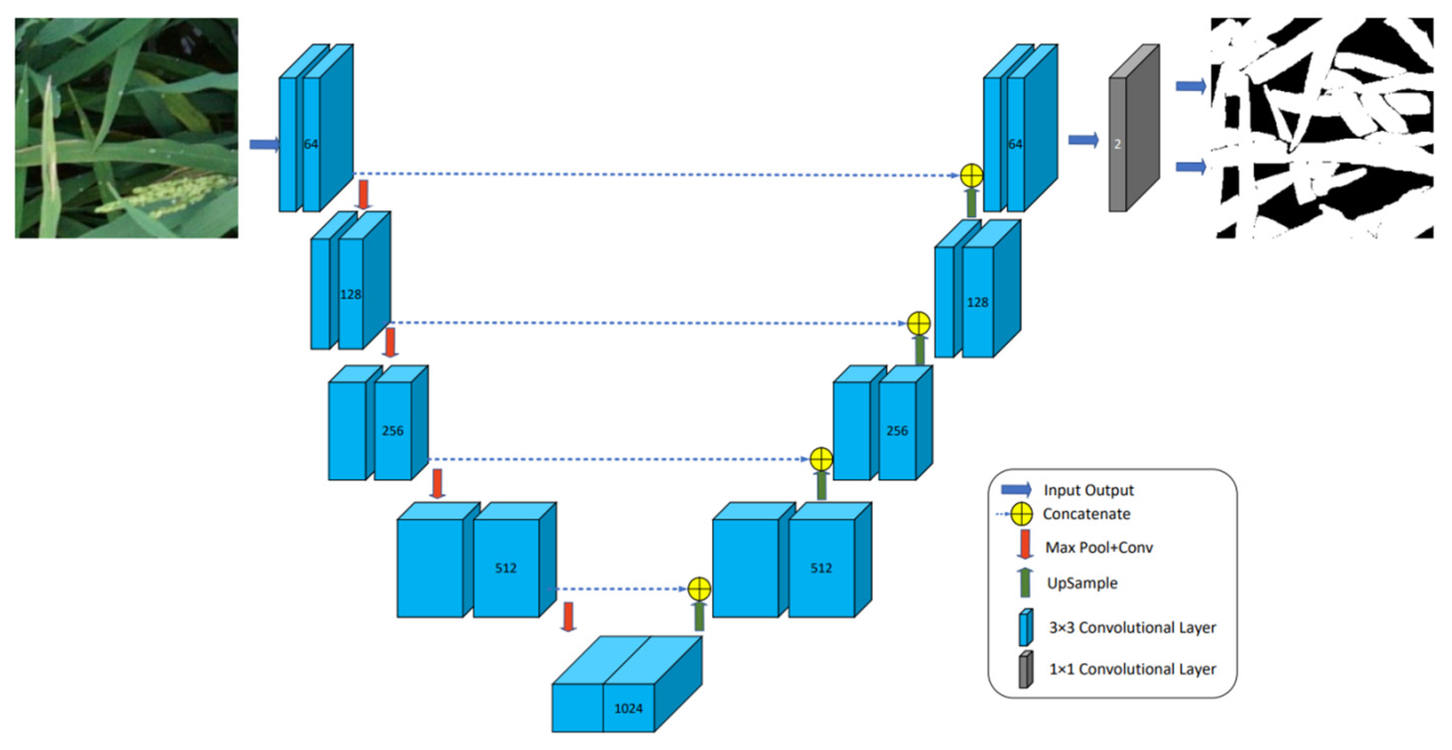
3.1.1. U-Net Network

The U-Net network is a widely used classical network in the computer vision field. The structure of U-Net consists of symmetric upsampling and downsampling segments, and the upsampling and downsampling segments are connected by a jumping connectivity layer. Because of this symmetric arrangement, the network forms a U-shaped structure and is thus named the U-Net network. The core concept of the U-Net network is to utilize a convolutional neural network to extract key characteristics from the input image and then recover the spatial resolution of the image through the upsampling operation in the decoder part and combine it with the high-resolution feature information in the encoder to achieve accurate image segmentation. In the training process, the training set of rice leaf images is input for training, and the leaf segmentation results are output. This process can be regarded as an adaptive image segmentation method. By continuously optimizing the model parameters, the accuracy and robustness of segmentation are progressively enhanced, resulting in segmentation outcomes that more closely approximate the true morphology of leaves. Ultimately, leaf segmentation images are obtained. Figure 4 illustrates the architectural diagram of the U-Net network.

The encoder extracts feature maps at four different scales through four identically structured submodules, each of which consists of a convolutional layer succeeded by a rectified linear unit (ReLU) activation function and a 2 ∗ 2 maximum pooling layer with a step stride of 2 used for downsampling, whose main role is to extract characteristics from the image and to steadily reduce the resolution of the characteristic maps.

The U-Net network convolutional layer formula is expressed as follows:

$$Y^{\mathrm{k}}={\displaystyle \sum _{i\in M}{I}_i^{k-1}}\ast u_i^k+v^k$$

(1)

$$I^{\mathrm{k}}=f(Y^k)$$

(2)

The pooling layer equation is expressed as follows:

$$Y^{\mathrm{k}}={\xi }^{k}down(I^{k-1})+v^k$$

(3)

$$I^{\mathrm{k}}=f(Y^k)$$

(4)

where $f\left(·\right)$ denotes the activation function, $I^k$ denotes the output of the kth convolutional layer, $Y^k$ is the neuron state of the kth convolution, $u_i^k$ and $v^k$ denote the filter matrix and bias matrix, respectively, and M is the feature map. The structure of the decoder is symmetric to that of the encoder and consists of upsampling the characteristic map by combining the characteristic map from the encoder path via 2 × 2 upward convolutions and two 3 × 3 convolutional layers, each succeeded by a ReLU activation function. In the rice leaf segmentation task, the decoder part gradually restores the deep feature maps extracted through the encoder to the same spatial resolution as the input image to achieve accurate pixel-level segmentation of the rice leaves.

3.1.2. Evaluation Indicators

To conduct an accurate evaluation of the segmentation performance of U-Net, this study uses precision and the mean intersection over union (MIoU) as the evaluation indices of network segmentation performance. The MIoU metric measures the proportion of intersections and concatenations of predictions and true labels in each category and is quantified separately for each category, and the final value is the average of these proportions for all categories. This approach effectively evaluates the overlapping regions between the predicted boundaries and actual annotations, thereby enabling a complete assessment of model performance.

$$Precision={\displaystyle \frac{TP}{TP+FP}}$$

(5)

$$MIoU={\displaystyle \frac{1}{k+1}}{\displaystyle \sum _{i=0}^k\frac{TP}{TP+FN+FP}}$$

(6)

where k+1 indicates the total number of categories (including background), TP denotes the pixels that have been correctly classified as part of the target category, TN denotes the pixels that are accurately categorized as nonmembers of the target category, FP denotes the pixels erroneously classified as part of the target category, and FN indicates the pixels incorrectly classified as not part of the target category.

3.2. Two-Phase Leaf Color Feature Optimization Approach

On the basis of the segmented image of the rice leaves, this study extracted the feature values of the rice leaves in the RGB and the HSI color spaces. The RGB color space serves as a color model founded on the additive synthesis of red, green, and blue color channels, which has become the most common standard in image processing, and the values of each channel can be extracted and combined as color feature parameters. To expand the color feature parameters, RGB is converted to the HSI color space, which can separate color information (H, S) from grayscale information (I), and saturation (S) and brightness (I) can help to differentiate the purity and lightness of the colors of different objects. The gray mean (gray) can effectively reflect the average brightness level of an image by calculating the average of the gray values of all the pixels in the image. In addition, the DGCI is strongly correlated with the chlorophyll content [41] via the following equation:

$$DGCI=\left[\left(H-60\right)/60+\left(1-S\right)+\left(1-V\right)\right]/3$$

(7)

$$H=\left\{\begin{array}{c}60\times \left({\displaystyle \frac{G-B}{\max \left(RGB\right)-\min \left(RGB\right)}}\right),\max \left(RGB\right)=R\\ 60\times \left(2+{\displaystyle \frac{B-G}{\max \left(RGB\right)-\min \left(RGB\right)}}\right),\max \left(RGB\right)=G\\ 60\times \left(4+{\displaystyle \frac{R-G}{\max \left(RGB\right)-\min \left(RGB\right)}}\right),\max \left(RGB\right)=B\end{array}\right.$$

(8)

$$S={\displaystyle \frac{\max \left(RGB\right)-\min \left(RGB\right)}{\max \left(RGB\right)}}$$

(9)

$$V=\max \left(RGB\right)$$

(10)

On the basis of the above discussion of different color spaces and prior knowledge [19,22], 26 color characteristic values were selected as experimental data in this study.

Table 1. List of color feature names.

Color Feature	Feature Names
R	Mean value of red in RGB color space
G	Mean value of green in RGB color space
B	Mean value of blue in RGB color space
H	Average color tone in HSI space
S	Average saturation of HSI space
I	Average brightness of the HSI space
r = R/(R + G + B)	Red standardized value
g = G/(R + G + B)	Green standardized value
b = B/(R + G + B)	Blue standardized value
g − b	Difference between green and blue standard values
g − r	Difference between green and red standard values
r − b	Difference between red and blue standard values
2 g − b − r	Normalized super green value
EXG = 2G − B − R	Ultra green indicator
(G − R)/(G+R)	The ratio of the green–red difference to the green–red sum
R/G	Red to green ratio
G/R	Green to red ratio
R/B	Red to blue ratio
G/B	Green to blue ratio
B/G	Blue to green ratio
G − B	The difference between green and blue
R − B	The difference between red and blue
G − R	The difference between green and red
R + G + B	The sum of red and green and blue
DGCI	Dark green color index
Gray	Grayscale average

presents the specific color features.

The total number of selected rice leaf color eigenvalues was 26, which would require 2²⁶ evaluations if all possible combinations were evaluated directly, which is many computations, and these characteristic parameters may be completely uncorrelated with the chlorophyll content. Therefore, the PCC method was first used for the initial screening to evaluate the correlation between each feature and the leaf’s SPAD value, sieve out the feature values with strong correlation, and reduce the number of unnecessary calculations. On the basis of preliminary screening, to further improve the accuracy of feature selection, an RF model is applied to ascertain the significance ranking of each feature, and recursive feature elimination is used to perform fine screening and ultimately achieve leaf color feature preference.

3.2.1. Pearson Correlation Coefficient Method

The PCC is employed to assess the level of linear relationship between two variables, x and y. When a variation in one variable induces a corresponding variation in another variable, they are said to be correlated. The formula is as follows:

$${\rho }_{X,Y}={\displaystyle \frac{\mathrm{cov}(X,Y)}{{\sigma }_X{\sigma }_Y}}={\displaystyle \frac{E(XY)-E(X)E(Y)}{\sqrt{E(X^2)-E^2\left(X\right)}\sqrt{E(Y^2)-E^2\left(Y\right)}}}$$

(11)

where cov denotes the covariance, $\sigma$ is the standard deviation, and (X,Y) is the true value of the two variables. The PCC lies between −1 and 1. Positive values indicate a positive relationship, and to determine the strength of the relationship, values closer to 1 reveal a more significant positive dependence between the two variables, whereas conversely, values closer to 0 imply a weakening of the relationship and a relative increase in independence. Negative values reflect a negative relationship, and in the same way, the closer the value is to −1, the stronger the negative dependence between the two variables. The closer that the absolute value of the p value is to 1, the more correlated the variables are. The correlation coefficients and correlations are shown in

Table 2. Relationships between correlation coefficients and correlations [42].

Absolute Value of Correlation Coefficient	Relevancy
0.8~1.0	High correlation
0.6~0.8	Strongly correlation
0.4~0.6	Moderate intensity correlation
0.2~0.4	Weak correlation
0.0~0.2	Minimally correlation

.

3.2.2. Recursive Feature Elimination

RFE is a feature selection algorithm used to reduce feature dimensions and select the best subset of features. It is an iterative algorithm based on ML models that can be used to select features that have the greatest predictive power for the target variable. In this work, RF-RFE is selected as the method for the second fine screening of the optimal feature subset, and its basic process is to input the feature subset initially screened by Pearson’s correlation coefficient into the random forest model for feature importance ranking and then train it in the random forest model by eliminating a feature with the least importance from the feature set in each iteration, which then progressively recurs until the feature set is empty. After each iteration, the results of this iteration are evaluated via a hierarchical cross-validation method, in which the sample data are divided into 5 equal parts, of which 4 are used as training data and 1 is used as test data, and the average accuracy of the 5 results is considered the accuracy of this iteration. All the results obtained in the process are compared and analyzed to derive the optimal feature set, which is then used as an input to the inversion model.

3.3. Inversion Modeling and Accuracy Evaluation

In this study, all the sample data of the obtained color eigenvalues were split into training and test sets at a ratio of 7:3. Four commonly employed ML methods were used for modeling, namely, the RF, SVR, BPNN, and XGBoost models. The grid search method [43] is adopted for parameter optimization. The optimal parameters are found by traversing all possible values of the parameter combinations in the grid. The optimal inversion model for chlorophyll content was selected on the basis of the analysis of the evaluation indices.

3.3.1. Random Forest Regression

RF is an ensemble learning methodology that enhances model accuracy and robustness through the construction of multiple decision trees and the aggregation of their predictions. During the training process, the random forest generates diverse decision trees through two kinds of randomness. First, random sampling with putback is performed on the training dataset to generate several different subsets. Specifically, n samples are randomly drawn from the original dataset to form the training subset $D_i$; second, when each node of the decision tree is split, a feature subset is randomly selected from all the features for the best split. Assuming that the original feature space contains p features, during node splitting, m features (m < p) are randomly selected among these p features, and the optimal splitting feature is chosen among these features; this approach can effectively mitigate the overfitting problem of a single decision tree. Upon entering the prediction phase, the random forest algorithm synthesizes the predictive outcomes from multiple decision trees to derive the final prediction, thereby achieving enhanced robustness and accuracy in predictive performance.

In this study, the number of decision trees in the RF model is set to 100, and the minimum number of cotyledon nodes is 5. The out-of-bag data error rate is used as an evaluation metric for variable importance analysis during the training process. First, for each decision tree in the random forest, the corresponding OOB is used to calculate the error, which is recorded as ε₁; second, noise interference is randomly added to feature I of all samples of OOB, and the OOB error is calculated again, which is recorded as ε₂; as the prediction accuracy of the OOB data decreases to a certain extent after noise is added to feature I, assuming that there are T trees in the random forest. Then, the importance of feature I can be calculated by Σ(ε₁ − ε₂)/T; the larger the value, the greater the impact of feature I on the sample regression results, the greater the importance.

3.3.2. Support Vector Regression

SVR, which is based on SVM, is commonly employed in regression analysis as a supervised learning algorithm. The SVR algorithm makes use of kernel functions to map the original data into a higher-dimensional feature space, thereby rendering the data distribution more amenable to fitting by linear regression models, consequently simplifying the solution of regression problems. The core idea is to find a regression function (like a hyperplane) in the feature space that meets the constraint conditions as much as possible, requiring the distance (i.e., error) from most data points to the function to remain within the preset tolerance range while punishing the points beyond the range to avoid the model’s overfitting of abnormal data points. The SVR algorithm has excellent generalization capabilities and exhibits some robustness to outliers. The kernel function selected for the model in this study is the radial basis function kernel; the final setting of the error term penalty coefficient is 1, and the kernel function coefficient is 0.01.

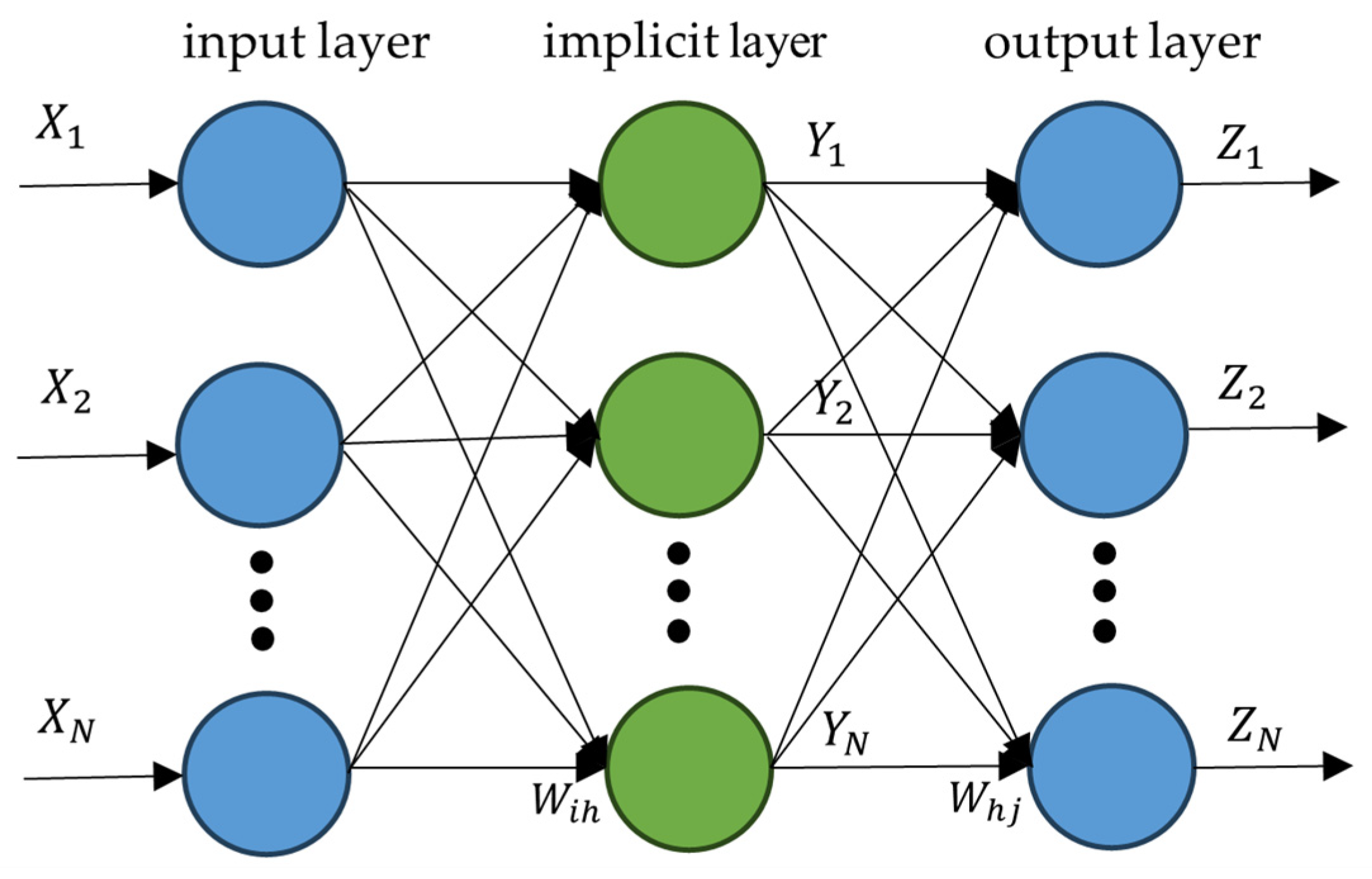
3.3.3. Backpropagation Neural Network

The backpropagation neural network learns through forward transmission and backpropagation. When transmitting forward, the input signal is processed by one or more hidden layers and then transmitted to the output layer. If the output is incorrect, the error propagates backward, and the weights are adjusted layer by layer to optimize the network performance. The number of iterations in the network training parameters is 1000, the error threshold is 10⁻⁶, the learning rate is set to 0.01, and the BPNN structure is shown below (Figure 5).

3.3.4. Extreme Gradient Boosting (XGBoost)

The extreme gradient boost (XGBoost) algorithm is also an ensemble learning algorithm. Its core idea lies in using gradient boost technology to gradually train multiple weak learners. In each round of iteration, the algorithm corrects the residuals of the previous round of the model and optimizes each weak learner via weighted learning and gradient descent methods. Furthermore, this algorithm performs second-order Taylor expansion on the loss function and introduces a regularization term, effectively avoiding the overfitting problem.

XGBoost uses k decision trees as weak learners, and the general formula of its prediction results is as follows.

$${\widehat{y}}_i=\varphi (x_i)={\displaystyle \sum _{k=1}^k{f}_k(x),} f_k\in F$$

(12)

${\widehat{y}}_i$ is the prediction result, $\varphi (x_i)$ is the predicted score of sample x_i, f_k is the CART decision tree, and F is the function space corresponding to the decision tree.

The formula of the loss function is as follows.

$$Obj(x)={\displaystyle \sum _{i=1}^{n}l(y_i,{\widehat{y}}_i)}+{\displaystyle \sum _{j=1}^k\Omega (f_i)},f_i\in f$$

(13)

where ${\displaystyle \sum _{i=1}^{n}l(y_i,{\widehat{y}}_i)}$ is the training error of sample x_i and where $\Omega (f_i)$ is the canonical term for the jth tree.

The final model optimization results of this study through the grid search method are as follows: the learning rate is 0.04, the maximum depth is 3, the number of estimators is 200, and the proportion of subsamples is 0.8.

3.3.5. Evaluation Indicators

The research employs two parameters, namely R² and RMSE, as evaluation indicators for the SPAD inversion model. R² is employed to evaluate the goodness of fit of the regression model coefficients and takes a value between 0 and 1. The closer the value is to 1, the better the fit. The RMSE is a quantitative indicator of the deviation between the actual and predicted values. A smaller RMSE value implies better model prediction performance.

$$R^2=1-{\displaystyle \frac{{\displaystyle {\sum }_{i=1}^n{(X_i-Y_i)}^2}}{{\displaystyle {\sum }_{i=1}^n{(X_i-\overline{X})}^2}}}$$

(14)

$$RMSE=\sqrt{{\displaystyle \frac{{\displaystyle {\sum }_{i=1}^n{(Y_i-X_i)}^2}}{n}}}$$

(15)

where $X_i$ and $Y_i$ are the measured and predicted values, respectively; $\overline{X}$ represents the mean of the observed values; and n represents the sample size.

4. Results

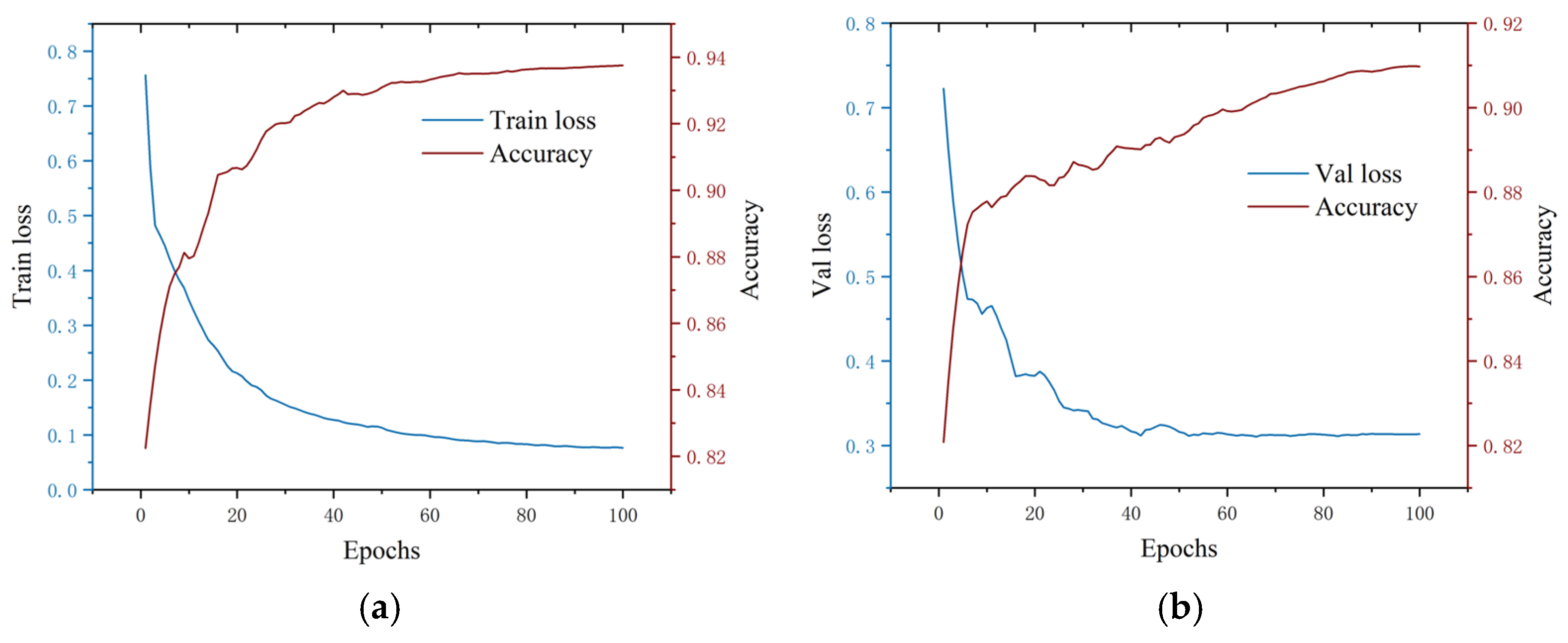
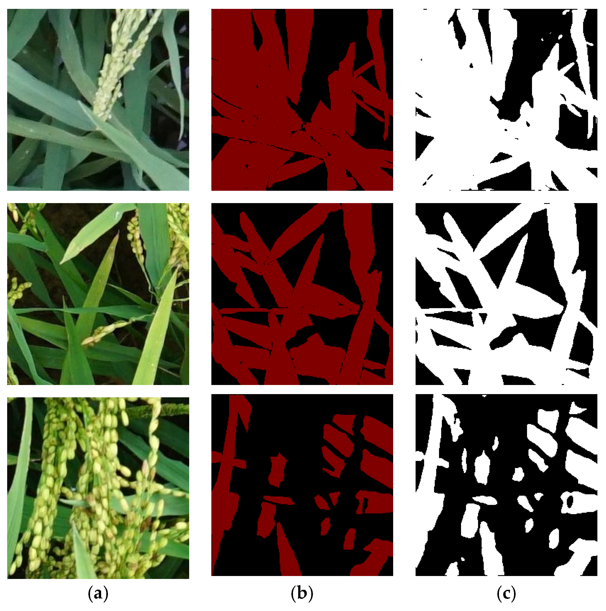
4.1. Rice Leaf Segmentation Model Training and Prediction

The rice leaf dataset is input into the U-Net segmentation network for image segmentation. The initial learning rate was set to 0.01, and the number of epochs was 100. In this study, L2 regularization is employed to prevent overfitting, and the weight decay coefficient is set at 0.0001. The model was trained, the MIoU was 88.23, and the loss and accuracy graphs are shown in Figure 6.

In Figure 6a, the training loss curve is high in the initial stage and then decreases, especially within the first 20 epochs. This phenomenon indicates that the model quickly learns effective rice leaf features in the early stages, resulting in a significant reduction in error. As training continues, the decrease in the loss value gradually decreases and plateaus after nearly 100 epochs, indicating that the optimization of the segmentation model is close to convergence. During the late stage of training, the loss value is low, indicating that the model can fit the training data better and effectively reduce the prediction error. The training accuracy curve shows an opposite trend to that of the loss value curve. In the initial stage, the accuracy is low and increases rapidly within the first 30 epochs, indicating that the model rapidly improves its classification ability in a short period. Thereafter, the rate of increase in accuracy gradually slowed and stabilized during subsequent training, eventually reaching a high level close to 0.937. In Figure 6b, the validation loss curve shows a similar trend. In the initial stage, the validation loss is high, but it gradually decreases with an increasing number of epochs and plateaus after approximately 40 epochs. Similarly, the validation accuracy curve shows that the model’s performance on the validation set gradually improved and stabilized after approximately 50 epochs, eventually reaching a level close to 0.91. The model can better handle the task of segmentation of rice leaves and can accurately predict the boundary between the leaf region and the background region, which reduces the number of cases of missegmentation and missed segmentation.

Figure 7 shows the corresponding segmentation result graph. The segmentation results of the 256 × 256 pixel image basically match the corresponding labeled truthful image, indicating that the segmentation of rice spike images via the U-Net deep learning model is reliable.

4.2. Leaf Color Characteristics

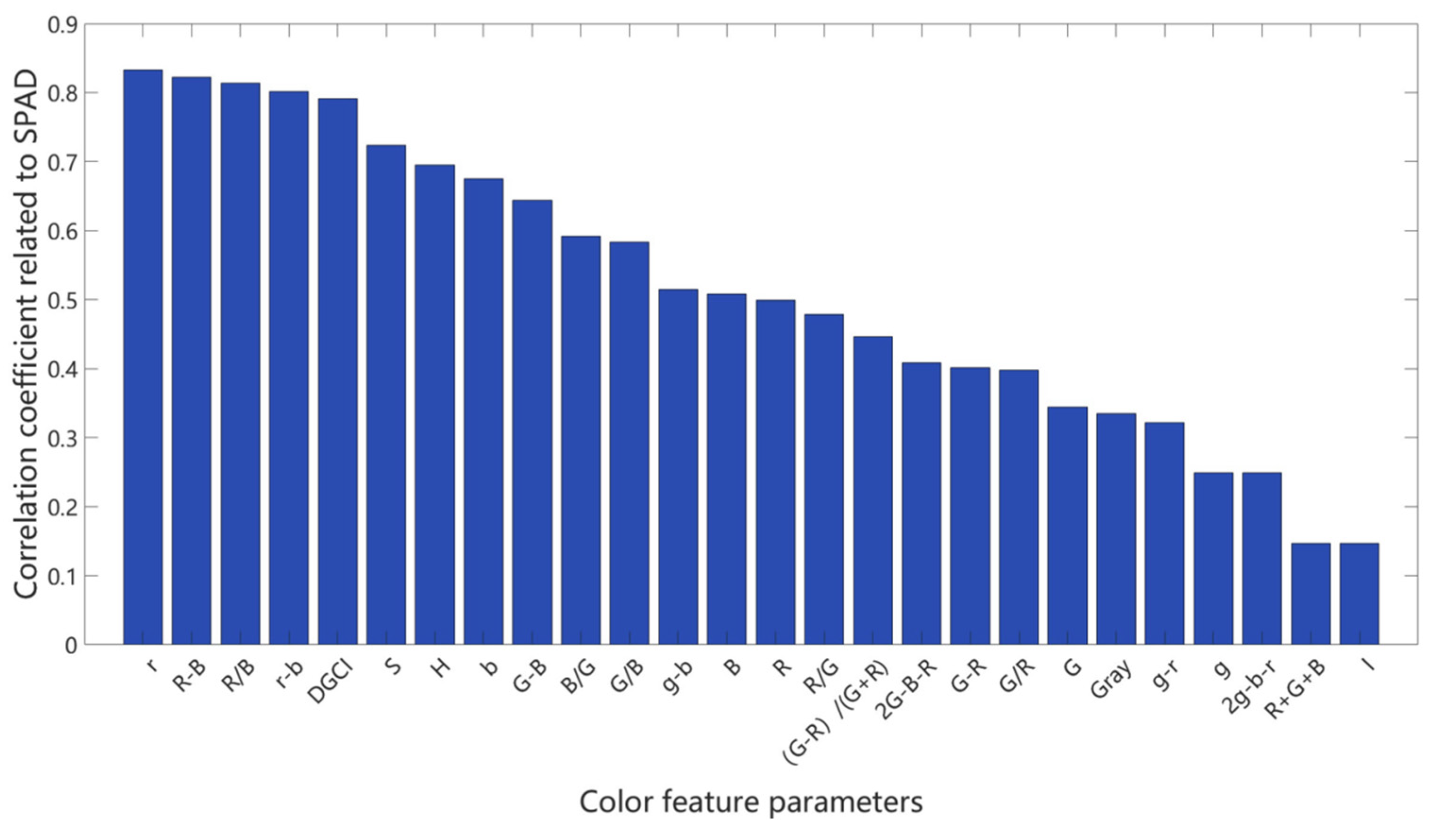
4.2.1. Pearson Coefficient Feature Selection

The 26 color feature values of all the rice leaf images were obtained on the basis of the color space, and the correlation coefficients between the original feature parameters and the SPAD values of the leaves were calculated via the Pearson correlation coefficient method. A higher coefficient indicates that the corresponding feature plays a more significant role in estimating leaf SPAD values. The following diagram illustrates the ranking of correlation magnitudes between 26 leaf color characteristic parameters and SPAD values.

The magnitude of correlation between each feature parameter and the leaf SPAD values is shown in Figure 8. To avoid the influence of parameters with a weak correlation to the SPAD value on the results, we selected features with an absolute correlation coefficient of no less than 0.6. A total of nine color characteristic parameters strongly correlated with leaf SPAD values were obtained via the Pearson coefficient method, which were r, R-B, R/B, r-b, DGCI, S, H, b, and G-B in descending order of magnitude, with absolute values of Pearson’s coefficients of 0.8325, 0.8228, 0.8141, 0.8013, 0.7909, and 0.7240, respectively, and 0.6950, 0.6754, and 0.6438, respectively.

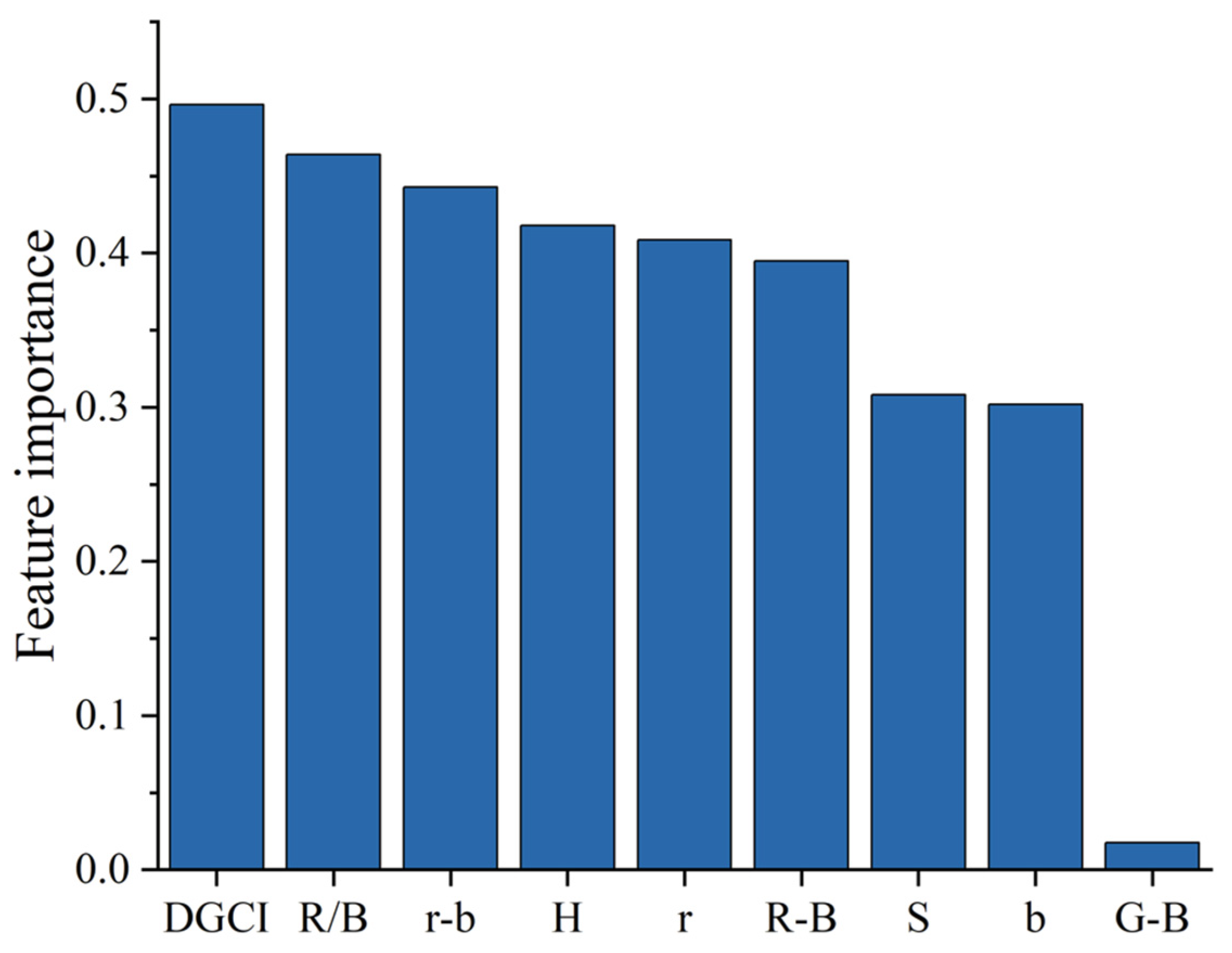
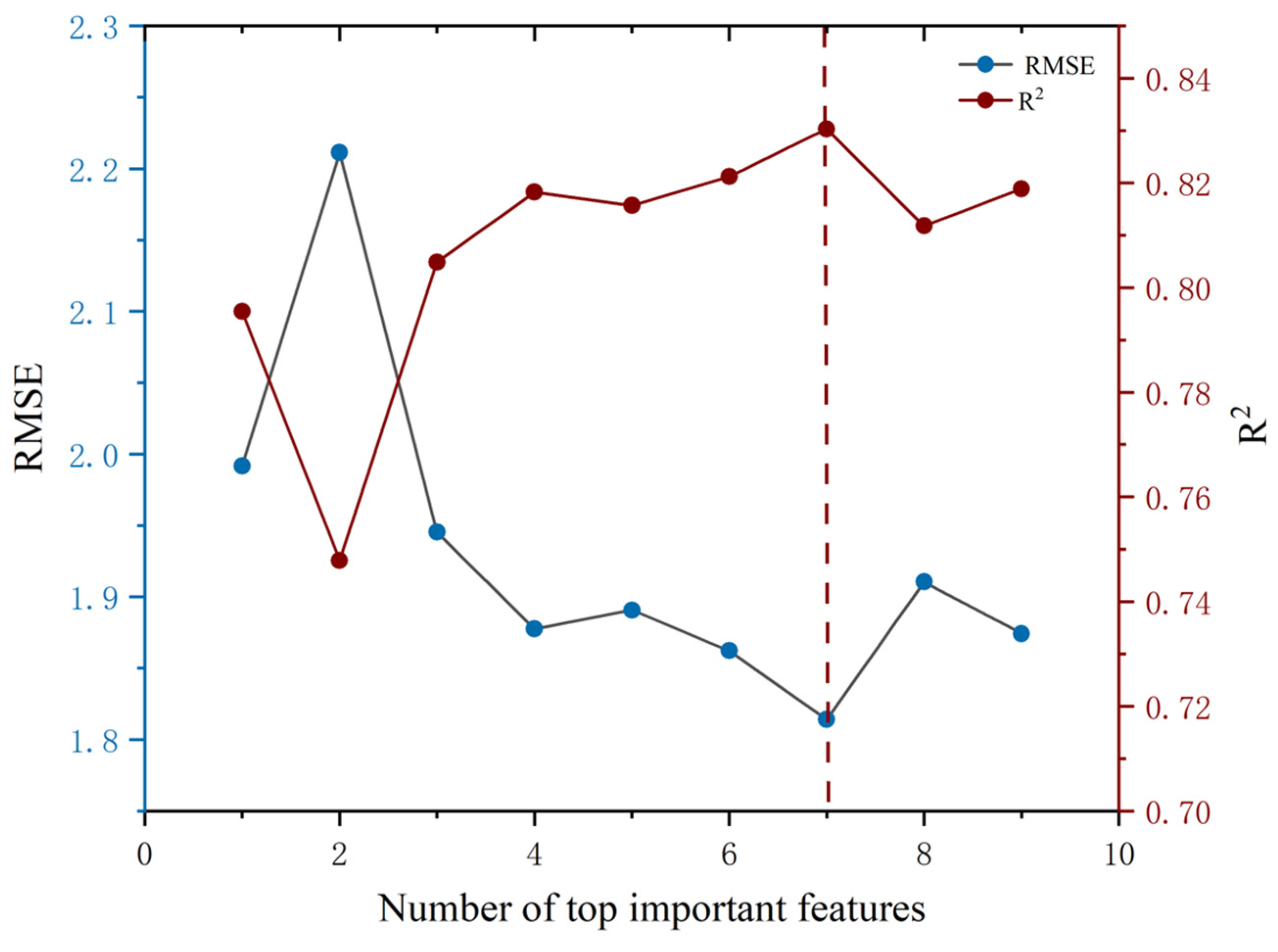
4.2.2. Random Forest-Based Recursive Feature Elimination

In this study, an RF-RFE method was employed to analyze the features initially selected through the aforementioned PCC approach, thereby determining the importance of each feature. The results of the importance ranking of the features via random forest are shown in Figure 9. On this basis, the RFE algorithm based on RF is utilized for iterative training in the model, and the variation curves of R² and RMSE in each round are obtained, as shown in Figure 10. As shown in Figure 10, the RMSE fluctuates more when the number of features is lower, indicating that the model is less stable, and with an increasing number of features, the RMSE shows a decreasing trend and reaches a relative minimum of 1.814 at seven features, indicating that the model’s prediction error is the smallest at that moment and that the performance is optimal. The R² serves as a crucial indicator for evaluating model fit, with values approaching one signifying a more robust and accurate model. When the number of features is increased to seven, R² reaches a peak of 0.830, indicating that the model currently has the strongest ability to fit the data. As the number of color features increases, the improvement in R² is not significant and even slightly decreases, which may be due to the introduction of redundant features leading to overfitting. Therefore, seven characteristic parameters, S, R-B, r, H, r-b, R/B, and DGCI, which can effectively predict the trend of leaf SPAD values, were selected.

4.3. Machine Learning-Based Inversion Model for SPAD Values

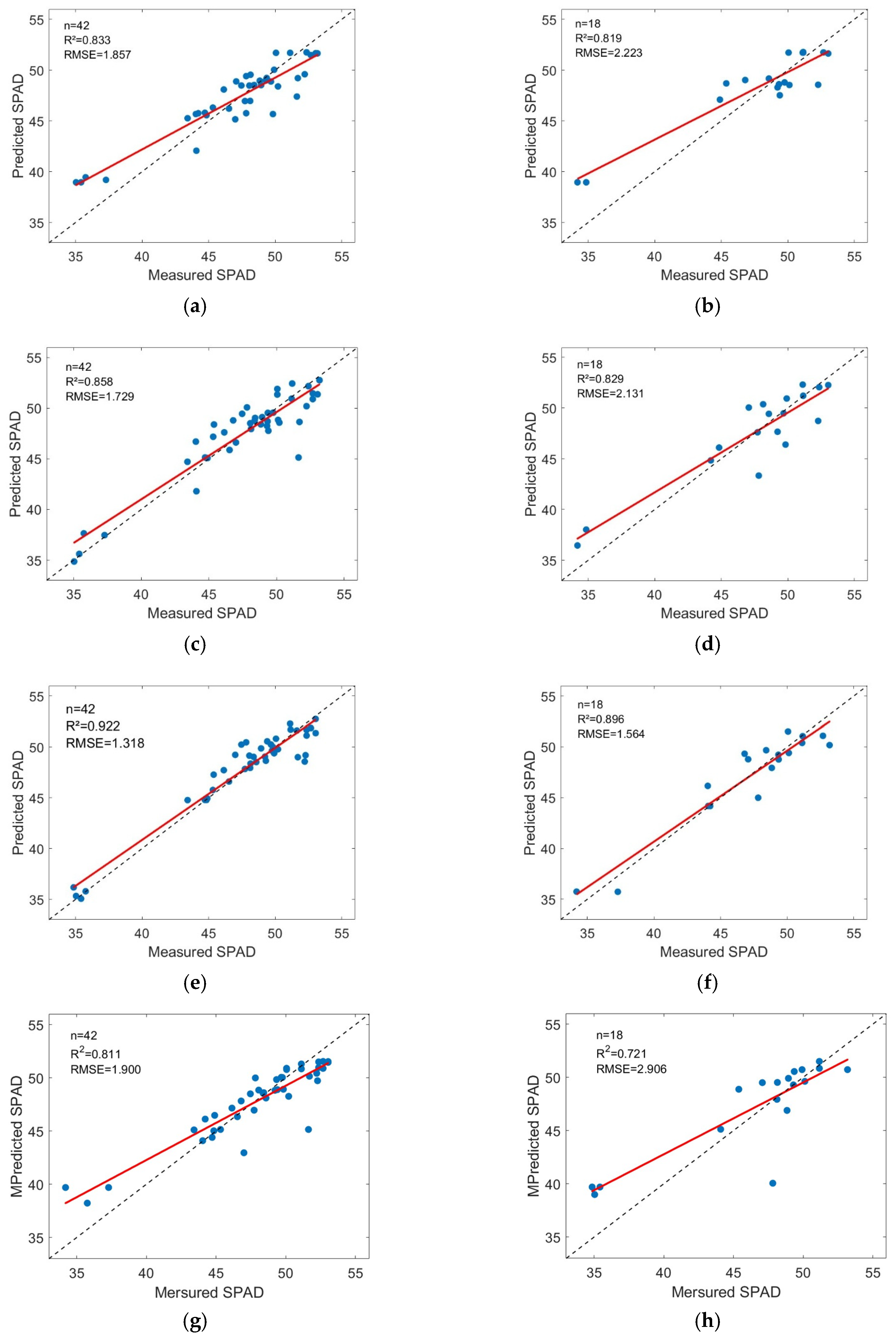
4.3.1. Machine Learning-Based Inversion and Accuracy Verification of SPAD Values

The RF algorithm, SVM regression, and BPNN were used to model the SPAD and the seven features preferred by the two-phase features. The research utilized a total of 60 samples, which were divided into training and test sets at a ratio of 7:3. The training set and test set consisted of 42 samples and 18 samples, respectively. Inverse modeling was performed via a training set based on the RF algorithm, SVM regression, and a BPNN, and the accuracy of the model was validated via a test set.

As shown in Figure 11, the training set R² values of the four models, RF, SVM, BPNN, and XGBoost, are 0.833, 0.858, 0.922, and 0.811, with RMSEs of 1.857, 1.729, 1.318 and 1.900, respectively, and the test set R² values are 0.819, 0.829, 0.896, and 0.721, with RMSEs of 2.223, 2.131, 1.564 and 2.906, respectively. By comparing the values of R² and RMSE, the BPNN yielded the best inversion results, while the inversion results of the RF and the SVM model were closer, with the SVM model slightly outperforming the RF model, but the difference between the two was not significant. The XGBoost model is slightly less effective than the RF and SVR models, but it can still achieve the inversion of SPAD values relatively well. Overall, the BPNN performed best in terms of both training and validation set accuracy, and the inverse model of the chlorophyll content SPAD value based on the BPNN could effectively predict the trend of the leaf SPAD value.

To further verify the efficacy of the rice leaf segmentation method based on U-Net in SPAD value inversion, this study inputs both the original leaf images and the rice leaf segmentation images obtained via the K-means algorithm (Figure 12) into the BPNN for SPAD value inversion. A comparative analysis of the inversion accuracies of the three types of SPAD values was subsequently conducted.

From Figure 12e, the inversion accuracy of the SPAD values based on the original leaf image R² is only 0.289, and the prediction accuracy of the model is too low because the interference of the rice spike and background affects the accuracy of the color eigenvalue extraction. In Figure 12f, which is based on the rice leaf segmentation image via the K-means algorithm, the SPAD value inversion R² value is 0.587, and the model fit is low. This is because the K-means clustering algorithm fails to effectively distinguish the leaf blade from the rice spike and the background in leaf segmentation and fails to accurately segment the leaf blade region, and the resulting deviation of the color eigenvalues leads to inaccurate data input into the model, which affects the inversion accuracy of the SPAD values. In summary, the use of the U-Net network segmentation of rice leaves can invert rice SPAD values with high accuracy.

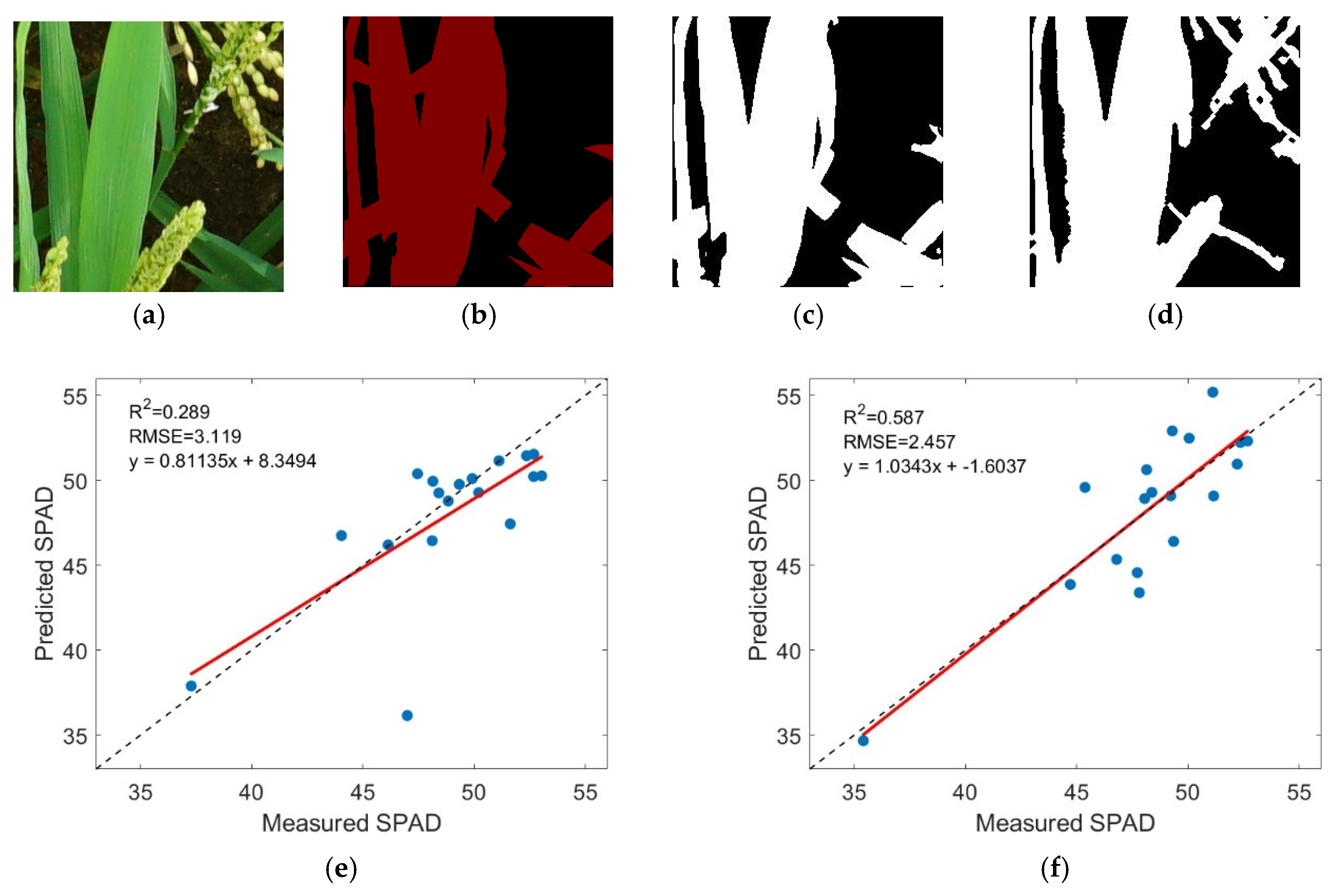
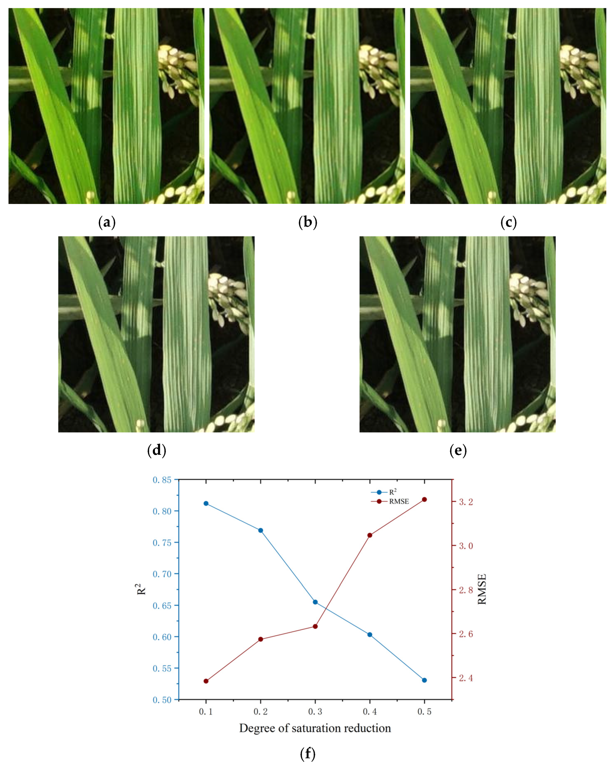
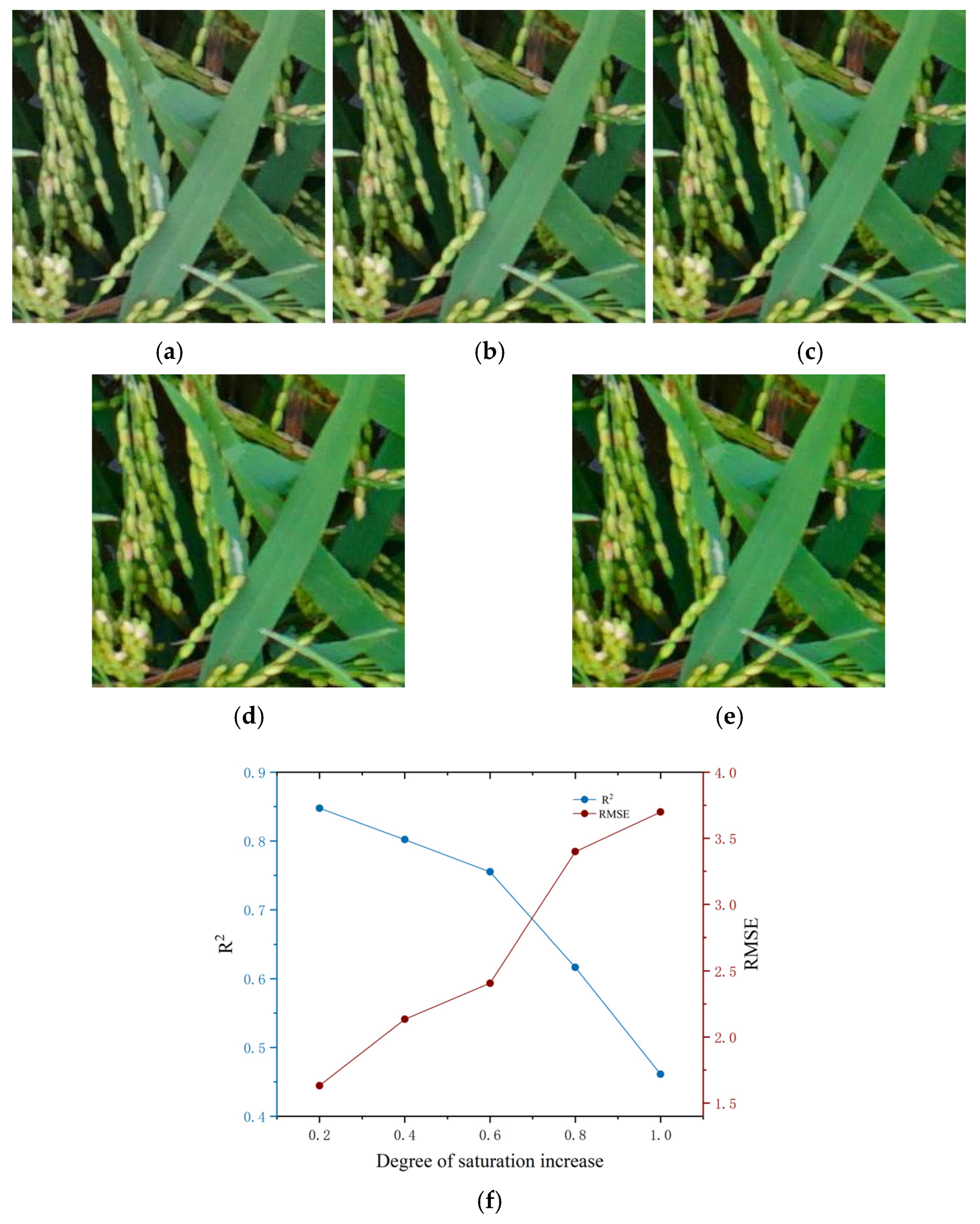
4.3.2. Comparison of the Inversion Accuracy of SPAD Values Under Different Image Qualities

To validate the robustness of the inversion model, three types of processing were carried out on the leaf images, namely, two weakening processing steps and one strengthening processing step. The first is to use Gaussian blur technology to simulate the reduction in image sharpness due to the lens swing when shooting images and set different Gaussian blur standard deviations (Sigma) to simulate different degrees of blur; a larger Sigma value means a greater degree of blurring. Second, a method of reducing image saturation is used to simulate low light in a field environment, and various low light scenarios are simulated by setting different levels of saturation reduction ratios. Third, the method of increasing the image saturation is adopted to simulate the situation of excessive light in the field environment, and various scenarios of excessive light are simulated by setting different saturation enhancement ratios. After the original blade image was input into the U-Net segmentation model, the color feature values of the corresponding blade parts were accurately extracted for the above-processed blade images (Figure 13). These feature values were input into the BPNN model for training, and the performance of the SPAD value inversion model was constructed and evaluated.

As shown in Figure 13, when the Sigma value is 0.5, the R² value of the model is close to 0.84, and the RMSE is lower, which indicates that the model can extract the SPAD change rule more accurately under the condition of low fuzziness. When the Sigma value increases to 1.5–2.5, the R² value decreases significantly and approaches 0.7, whereas the RMSE increases gradually, which indicates that the predictive accuracy of the model decreases gradually with an increasing degree of fuzziness. At a Sigma value of 3, R² decreases to 0.65, and RMSE increases to 3.4, which indicates that in the presence of higher levels of ambiguous interference, the color eigenvalues of the leaves are affected, thereby leading to inaccurate prediction of SPAD by the model. Nonetheless, the model proposed in this study is still able to provide some degree of predictive power at higher levels of ambiguity, and even with a Sigma value of 3, the model is still able to approximately predict the SPAD value. This indicates that the inversion model has some robustness and can adapt to the interference of image blurring to some extent, providing more reasonable SPAD inversion results.

The change in accuracy of the chlorophyll SPAD inversion model under reduced image saturation is demonstrated in Figure 14. The simulation accuracy of the model clearly decreased as the degree of image saturation reduction increased. When the degree of image saturation reduction is 0.1, the R² value of the model is close to 0.80, indicating that the model is capable of accurately inverting the SPAD value at higher image saturation. When the degree of leaf image saturation reduction is in the range of 0.2–0.5, the R² value gradually decreases to a minimum of 0.53, whereas the RMSE gradually increases to 3.2, which indicates that the prediction accuracy of the model is significantly reduced at this time. When the degree of image saturation is reduced to 0.4, the R² of the model is reduced to 0.6, and the prediction accuracy decreases. However, the model is still able to extract effective features from the changing color eigenvalues and make predictions, which shows that the proposed model has a certain robustness and adaptability. These findings indicate that the proposed inversion model is still effective at predicting the chlorophyll content when the image saturation is reduced within a certain range.

As shown in Figure 15, the accuracy variation in the chlorophyll SPAD inversion model under the condition of increased image saturation is presented. With an increasing saturation degree of the image, the performance of the model clearly decreases. Specifically, R2 gradually decreases with increasing saturation, from a high value close to 0.85 to a low value of approximately 0.45. In particular, when the increase in saturation exceeds 0.8, the downward trend is more significant. When the degree of increase in image saturation is 0.2, the R² value of the model is close to 0.85, indicating that the model can accurately invert the chlorophyll SPAD value under this image saturation. When the degree of saturation increase in the leaf image is between 0.4 and 1.0, the R² value gradually decreases and decreases to a minimum of 0.46, whereas the RMSE gradually increases and reaches 3.6. This indicates that the prediction accuracy of the model gradually decreases at this time. When the degree of saturation increase exceeds 0.8, the prediction error increases significantly. This indicates that when the image saturation of the model is relatively high, the prediction accuracy decreases significantly. When the degree of increase in image saturation is 0.8, although the R² of the model decreases to 0.62 and the prediction accuracy decreases somewhat, the model can still extract effective features from the changing color feature values and make predictions, indicating that the proposed model has certain robustness and adaptability. This finding indicates that when the image saturation is increased within a certain range, the proposed inversion model can still effectively predict the chlorophyll content effectively.

5. Discussion

5.1. Important Role of Rice Leaf Segmentation via the U-Net Network for Accurate SPAD Extraction

The machine vision-based image processing method can quickly obtain chlorophyll content monitoring results, but the chlorophyll content obtained via this method is susceptible to the influence of the field environment on the image, especially the background soil or other components of the crop; therefore, the target leaf area needs to be accurately extracted before the chlorophyll content can be inverted. Most traditional machine vision-based chlorophyll content inversion methods are limited to single-leaf analysis under simple background conditions. This research focuses on rice leaf images under complex backgrounds and constructs a rice leaf segmentation model based on the U-Net network. The maximum MIoU reaches 88.23 after training, realizing the accurate segmentation of leaves under complex backgrounds. On the basis of the rice leaf segmentation images, the inversion of SPAD values via the BPNN effectively predicted the trend of the leaf SPAD values. In addition, the results of rice SPAD inversion via the U-Net network were compared with the results of SPAD value inversion via the original leaf images and the K-means algorithm in this study, which further verified the important role of rice leaf segmentation via the U-Net network for accurate SPAD extraction.

5.2. Construction and Robustness of SPAD Inversion Models

Owing to the excessive number of leaf color feature parameters, 26 feature parameters were initially selected as the sample dataset in this study. Considering that the direct application of the recursive feature elimination (RFE) method requires 26 iterations, there may be parameters that are not relevant to the chlorophyll content. Therefore, this study adopts a two-stage feature optimization method. First, the PCC-based method is used for preliminary screening, and the feature parameters with correlations with chlorophyll contents greater than 0.6 are retained. The RFE method is subsequently used to optimize the screened feature set, and a comparison of the prediction accuracies of different feature combinations reveals that the optimal feature parameter combination contains 7 parameters. This combination affects the model performance. The finalized feature parameter combinations are S, R-B, r, H, r-b, R/B, and DGCI. An effective feature set is provided for the data of the subsequent ML model. Furthermore, to explore the performance of the chlorophyll content prediction model under different image qualities, two weakening treatments were applied to the leaf images in this study, and an analysis of the accuracy of SPAD inversion on the basis of the above weakened images was performed. In the case of reduced image sharpness due to lens wobbles, the R² of the model was 0.647 when the Sigma of the leaf image was increased to 3. In the case of low light in the field background, the R² of the model was 0.603 when the leaf saturation decreased to 0.4. In summary, the predictive ability of the model decreases as the image quality deteriorates, but certain features can still be extracted from the image for relatively accurate chlorophyll SPAD prediction, indicating that the model is robust to image blurring and saturation degradation.

5.3. Limitations of This Study and Future Perspectives

Although the chlorophyll content inversion method that combines deep learning and feature optimization proposed in this paper achieves good prediction results in the study area, there are still some problems that urgently need to be studied. Although existing studies have shown that the U-Net network demonstrates high performance in the plant segmentation task [33,34], to further verify its superiority and explore other potential effective models (Mask-RCNN, DeepLabV3+, etc.), we plan to conduct more extensive comparative experiments in future research. A more comprehensive perspective is provided to examine the performance of different models in the task of rice leaf segmentation. There are still some fine regions in the rice leaf segmentation results that are not accurately recognized and segmented by the model, which may have some impact on the final chlorophyll content estimation results. To address the shortcomings of the existing U-Net segmentation model, further improvements in the segmentation model will be considered in the future by leading the attention mechanism to the model and optimizing the loss function. Furthermore, the sample size of the chlorophyll content data collected in this study was relatively limited, making it difficult to generalize the research conclusions to different environments. In the future, the sample space of SPADs will be expanded, and additional experiments, such as those involving shadows and leaf occlusions, will be conducted under real field conditions to further enhance the generalizability of the SPAD inversion model. Moreover, we focus on inverting SPAD values for different periods of rice growth (e.g., tillering, nodulation, tasseling, etc.) individually. Judging the growth of rice on the basis of the SPAD values of rice leaves in different periods can more accurately assess the health status of rice in different growth stages and thus provide better decision support for field management. Moreover, this technology can be used in real time by a drone equipped with AI-capable edge devices and can capture azimuthal images of the crop to achieve field implementation monitoring.

6. Conclusions

This study focuses on rice leaf images under complex backgrounds and proposes a nondestructive inversion method for the rice leaf chlorophyll content by integrating deep learning and feature optimization. SPAD inversion models for rice leaves based on RF, SVM, BPNN, and XGBoost were established, and the accuracy was verified. The results show that the overall performance of the SPAD model based on the BPNN is optimal, with R² and RMSE values of 0.896 and 1.564 on the test set, respectively, realizing high-precision prediction. Finally, through robustness tests on different low-definition and low-saturation images, the model is verified to be stable and reliable even under complex lighting conditions. In conclusion, this study offers strong technical support for fast, nondestructive, and precise monitoring of the chlorophyll content of crop leaves via machine vision.

References

1. Jang, Y.H.; Park, J.R.; Kim, E.G.; Kim, K.M. The Basic Helix-Loop-Helix Transcription Factor, Involved in Regulation of Chlorophyll Content in Rice. Biology 2022, 11, 1000. [Google Scholar] [CrossRef]
2. Zhai, W.G.; Li, C.C.; Cheng, Q.; Ding, F.; Chen, Z. Exploring Multisource Feature Fusion and Stacking Ensemble Learning for Accurate Estimation of Maize Chlorophyll Content Using Unmanned Aerial Vehicle Remote Sensing. Remote Sens. 2023, 15, 3454. [Google Scholar] [CrossRef]
3. Peng, J.; Xu, F.X.; Deng, K.; Wu, J.; Li, W.T.; Wang, N.; Liu, M.S. Spectral Differences of Tree Leaves at Different Chlorophyll Relative Content in Langya Mountain. Spectrosc. Spect. Anal. 2018, 38, 1839–1849. [Google Scholar]
4. Liu, H.H.; Lei, X.Q.; Liang, H.; Wang, X. Multi-Model Rice Canopy Chlorophyll Content Inversion Based on UAV Hyperspectral Images. Sustainability 2023, 15, 7038. [Google Scholar] [CrossRef]
5. Treder, W.; Klamkowski, K.; Sowik, I.; Maciorowski, R. Possibilities of Using Rgb-Based Image Analysis to Estimate the Chlorophyll Content of Micropropagated Strawberry Plants. Acta Sci. Pol. Hortorum Cultus 2021, 20, 105–115. [Google Scholar] [CrossRef]
6. Qin, R.; He, L.; Li, Y.X.; He, J.X.; Gao, J.; Yan, F.F.; Yu, Y.F.; Liao, K.W.; Lu, L.M.; Jian, S.C.; et al. Remote Sensing Inversion of Tobacco Spad Based on Uav Hyperspectral Imagery. In Proceedings of the IGARSS 2023-2023 IEEE International Geoscience and Remote Sensing Symposium, Pasadena, CA, USA, 16–21 July 2023; pp. 3478–3481. [Google Scholar] [CrossRef]
7. Cavallo, D.P.; Cefola, M.; Pace, B.; Logrieco, A.F.; Attolico, G. Contactless and non-destructive chlorophyll content prediction by random forest regression: A case study on fresh-cut rocket leaves. Comput. Electron. Agric. 2017, 140, 303–310. [Google Scholar] [CrossRef]
8. Yan, N.; Qin, Y.S.; Wang, H.T.; Wang, Q.; Hu, F.Y.; Wu, Y.W.; Zhang, X.D.; Li, X. The Inversion of SPAD Value in Pear Tree Leaves by Integrating Unmanned Aerial Vehicle Spectral Information and Textural Features. Sensors 2025, 25, 618. [Google Scholar] [CrossRef]
9. Lee, G.; Hwang, J.; Cho, S. A Novel Index to Detect Vegetation in Urban Areas Using UAV-Based Multispectral Images. Appl. Sci. 2021, 11, 3472. [Google Scholar] [CrossRef]
10. Lu, L.L.; Kuenzer, C.; Wang, C.Z.; Guo, H.D.; Li, Q.T. Evaluation of Three MODIS-Derived Vegetation Index Time Series for Dryland Vegetation Dynamics Monitoring. Remote Sens. 2015, 7, 7597–7614. [Google Scholar] [CrossRef]
11. Pradhan, S.; Bandyopadhyay, K.K.; Josh, D.K. Canopy reflectance spectra of wheat as related to crop yield, grain protein under different management practices. J. Agrometeorol. 2012, 14, 21–25. [Google Scholar] [CrossRef]
12. Ballester, C.; Brinkhoff, J.; Quayle, W.C.; Hornbuckle, J. Monitoring the Effects of Water Stress in Cotton Using the Green Red Vegetation Index and Red Edge Ratio. Remote Sens. 2019, 11, 873. [Google Scholar] [CrossRef]
13. Tian, B.Q.; Yu, H.L.; Zhang, S.L.; Wang, X.L.; Yang, L.; Li, J.Q.; Cui, W.H.; Wang, Z.S.; Lu, L.Q.; Lan, Y.B.; et al. Inversion of Cotton Soil and Plant Analytical Development Based on Unmanned Aerial Vehicle Multispectral Imagery and Mixed Pixel Decomposition. Agriculture 2024, 14, 1452. [Google Scholar] [CrossRef]
14. Chen, Z.Q.; Wang, L.; Bai, Y.L.; Yang, L.P.; Lu, Y.L.; Wang, H.; Wang, Z.Y. Hyperspectral Prediction Model for Maize Leaf SPAD in the Whole Growth Period. Spectrosc. Spect. Anal. 2013, 33, 2838–2842. [Google Scholar] [CrossRef]
15. Lu, Y.; Yang, H.Y.; Sun, A.Z. The Research of SPAD in Rice Leaves Based on Machine Learning. In Proceedings of the 2019 Chinese Automation Congress (CAC), Hangzhou, China, 22–24 November 2019; pp. 2163–2167. [Google Scholar] [CrossRef]
16. Song, J. Bias corrections for Random Forest in regression using residual rotation. J. Korean Stat. Soc. 2015, 44, 321–326. [Google Scholar] [CrossRef]
17. Guerrero, J.M.; Pajares, G.; Montalvo, M.; Romeo, J.; Guijarro, M. Support Vector Machines for crop/weeds identification in maize fields. Expert. Syst. Appl. 2012, 39, 11149–11155. [Google Scholar] [CrossRef]
18. Sun, B.; Sun, T.; Jiao, P.P. Spatio-Temporal Segmented Traffic Flow Prediction with ANPRS Data Based on Improved XGBoost. J. Adv. Transp. 2021, 2021, 5559562. [Google Scholar] [CrossRef]
19. Moghaddam, P.A.; Derafshi, M.H.; Shirzad, V. Estimation of single leaf chlorophyll content in sugar beet using machine vision. Turk. J. Agric. For. 2011, 35, 563–568. [Google Scholar] [CrossRef]
20. Sikakollu, P.; Dash, R. Ensemble of multiple CNN classifiers for HSI classification with Superpixel Smoothing. Comput. Geosci. 2021, 154, 104806. [Google Scholar] [CrossRef]
21. He, X.F.; Lv, X.G. From the color composition to the color psychology: Soft drink packaging in warm colors, and spirits packaging in dark colors. Color. Res. Appl. 2022, 47, 758–770. [Google Scholar] [CrossRef]
22. Hassanijalilian, O.; Igathinathane, C.; Doetkott, C.; Bajwa, S.; Nowatzki, J.; Esmaeili, S.A.H. Chlorophyll estimation in soybean leaves infield with smartphone digital imaging and machine learning. Comput. Electron. Agric. 2020, 174, 105433. [Google Scholar] [CrossRef]
23. Hong, S.L.; Jiang, Z.H.; Liu, L.Z.; Wang, J.; Zhou, L.Y.; Xu, J.P. Improved Mask R-CNN Combined with Otsu Preprocessing for Rice Panicle Detection and Segmentation. Appl. Sci. 2022, 12, 11701. [Google Scholar] [CrossRef]
24. Liao, J.; Wang, Y.; Yin, J.N.; Liu, L.; Zhang, S.; Zhu, D.Q. Segmentation of Rice Seedlings Using the YCrCb Color Space and an Improved Otsu Method. Agronomy 2018, 8, 269. [Google Scholar] [CrossRef]
25. Zhang, Y.Q.; Xiao, D.Q.; Liu, Y.F. Automatic Identification Algorithm of the Rice Tiller Period Based on PCA and SVM. IEEE Access 2021, 9, 86843–86854. [Google Scholar] [CrossRef]
26. Singh, S.; Mittal, N.; Singh, H.; Oliva, D. Improving the segmentation of digital images by using a modified Otsu’s between-class variance. Multimed. Tools Appl. 2023, 82, 40701–40743. [Google Scholar] [CrossRef]
27. Han, C.Y. Improved SLIC imagine segmentation algorithm based on K-means. Cluster Comput. 2017, 20, 1017–1023. [Google Scholar] [CrossRef]
28. Miao, Y.L.; Li, S.; Wang, L.Y.; Li, H.; Qiu, R.C.; Zhang, M. A single plant segmentation method of maize point cloud based on Euclidean clustering and K-means clustering. Comput. Electron. Agric. 2023, 210, 107951. [Google Scholar] [CrossRef]
29. Zhang, J.H.; Gong, J.L.; Zhang, Y.F.; Mostafa, K.; Yuan, G.Y. Weed Identification in Maize Fields Based on Improved Swin-Unet. Agronomy 2023, 13, 1846. [Google Scholar] [CrossRef]
30. Zunair, H.; Ben Hamza, A. Sharp U-Net: Depthwise convolutional network for biomedical image segmentation. Comput. Biol. Med. 2021, 136, 104699. [Google Scholar] [CrossRef]
31. Wu, W.B.; Liu, G.J.; Liang, K.Y.; Zhou, H. Inner Cascaded U2-Net: An Improvement to Plain Cascaded U-Net. Cmes-Comp. Model. Eng. 2023, 134, 1323–1335. [Google Scholar] [CrossRef]
32. Zhang, J.H.; You, S.C.; Liu, A.X.; Xie, L.J.; Huang, C.H.; Han, X.; Li, P.H.; Wu, Y.X.; Deng, J.S. Winter Wheat Mapping Method Based on Pseudo-Labels and U-Net Model for Training Sample Shortage. Remote Sens. 2024, 16, 2553. [Google Scholar] [CrossRef]
33. Liu, G.Q.; Bai, L.; Zhao, M.Q.; Zang, H.C.; Zheng, G.Q. Segmentation of wheat farmland with improved U-Net on drone images. J. Appl. Remote Sens. 2022, 16, 034511. [Google Scholar] [CrossRef]
34. Zhang, S.W.; Zhang, C.L. Modified U-Net for plant diseased leaf image segmentation. Comput. Electron. Agric. 2023, 204, 107511. [Google Scholar] [CrossRef]
35. Kolhar, S.; Jagtap, J. Convolutional neural network based encoder-decoder architectures for semantic segmentation of plants. Ecol. Inform. 2021, 64, 101373. [Google Scholar] [CrossRef]
36. Boston, T.; Van Dijk, A.; Larraondo, P.R.; Thackway, R. Comparing CNNs and Random Forests for Landsat Image Segmentation Trained on a Large Proxy Land Cover Dataset. Remote Sens. 2022, 14, 3396. [Google Scholar] [CrossRef]
37. Yu, X.; Yin, D.M.; Nie, C.W.; Ming, B.; Xu, H.G.; Liu, Y.; Bai, Y.; Shao, M.C.; Cheng, M.H.; Liu, Y.D.; et al. Maize tassel area dynamic monitoring based on near-ground and UAV RGB images by U-Net model. Comput. Electron. Agric. 2022, 203, 107477. [Google Scholar] [CrossRef]
38. Yang, H.B.; Hu, Y.H.; Zheng, Z.Z.; Qiao, Y.C.; Zhang, K.L.; Guo, T.F.; Chen, J. Estimation of Potato Chlorophyll Content from UAV Multispectral Images with Stacking Ensemble Algorithm. Agronomy 2022, 12, 2318. [Google Scholar] [CrossRef]
39. Zhang, A.W.; Yin, S.N.; Wang, J.; He, N.P.; Chai, S.T.; Pang, H.Y. Grassland Chlorophyll Content Estimation from Drone Hyperspectral Images Combined with Fractional-Order Derivative. Remote Sens. 2023, 15, 5623. [Google Scholar] [CrossRef]
40. Hunt, E.R.; Daughtry, C.S.T. Chlorophyll Meter Calibrations for Chlorophyll Content Using Measured and Simulated Leaf Transmittances. Agron. J. 2014, 106, 931–939. [Google Scholar] [CrossRef]
41. dos Santos, C.L.; Roberts, T.L.; Purcell, L.C. Canopy greenness as a midseason nitrogen management tool in corn production. Agron. J. 2020, 112, 5279–5287. [Google Scholar] [CrossRef]
42. Zhao, X.; Zhao, Z.Y.; Zhao, F.N.; Liu, J.F.; Li, Z.Y.; Wang, X.P.; Gao, Y. An Estimation of the Leaf Nitrogen Content of Apple Tree Canopies Based on Multispectral Unmanned Aerial Vehicle Imagery and Machine Learning Methods. Agronomy 2024, 14, 552. [Google Scholar] [CrossRef]
43. Chen, H.Z.; Zhang, Z.J.; Yin, W.L.; Zhao, C.Y.; Wang, F.X.; Li, Y.F. A study on depth classification of defects by machine learning based on hyper-parameter search. Measurement 2022, 189, 110660. [Google Scholar] [CrossRef]
Figure 1. Experimental plot deployment and image acquisition. Experimental plot deployment (a) and image acquisition (b).
Agriculture 15 01270 g001
Figure 2. Image enhancement. (a) Original. (b) Mirror. (c) Fuzzy. (d) Enhanced saturation. (e) Gaussian noise. (f) Reduced contrast.
Agriculture 15 01270 g002
Figure 3. Technology roadmap.
Agriculture 15 01270 g003
Figure 4. U-Net network structure.
Agriculture 15 01270 g004
Figure 5. BPNN structure.
Agriculture 15 01270 g005
Figure 6. (a) Trend of the loss value and accuracy during the model training process. (b) Trend of the loss value and accuracy during model validation.
Agriculture 15 01270 g006
Figure 7. Projected results. (a) Raw images. (b) Labeled images. (c) Segmentation images.
Agriculture 15 01270 g007
Figure 8. Characterization results based on Pearson’s coefficient method.
Agriculture 15 01270 g008
Figure 9. Random forest-based feature importance analysis.
Agriculture 15 01270 g009
Figure 10. Recursive feature preference analysis.
Agriculture 15 01270 g010
Figure 11. Comparison of inverse models for chlorophyll content SPAD values. (a) RF training set. (b) RF test set. (c) SVM training set. (d) SVM test set. (e) BPNN training set. (f) BPNN test set. (g) XGBoost training set. (h) XGBoost test set.
Agriculture 15 01270 g011
Figure 12. Inversion of SPAD values for chlorophyll content under different partitioning scenarios. (a) Raw image. (b) Labeled image. (c) U-Net result. (d) K-means result. (e) Raw image SPAD inversion accuracy. (f) K-means segmentation SPAD inversion accuracy.
Agriculture 15 01270 g012
Figure 13. SPAD inversion for different blurring cases. (a) Sigma = 0.5 (b) Sigma = 1 (c) Sigma = 1.5 (d) Sigma = 2 (e) Sigma = 2.5 (f) Sigma = 3 (g) Accuracy of SPAD inversion under different fuzzy conditions.
Agriculture 15 01270 g013
Figure 14. SPAD inversion for different saturation reductions. (a) Saturation was reduced by 0.1. (b) Saturation was reduced by 0.2. (c) Saturation was reduced by 0.3. (d) Saturation was reduced by 0.4 (e) Saturation was reduced by 0.5. (f) SPAD inversion accuracy for different saturation reductions.
Agriculture 15 01270 g014
Figure 15. SPAD inversion for different saturation increase conditions. (a) Saturation increased by 0.1. (b) Saturation increased by 0.2. (c) Saturation increased by 0.3. (d) Saturation increased by 0.4. (e) Saturation increased by 0.5. (f) SPAD inversion accuracy for different increasing saturation conditions.
Agriculture 15 01270 g015