Article

Path Tracking Control of Agricultural Automatic Navigation Vehicles Based on an Improved Sparrow Search-Pure Pursuit Algorithm

1
College of Optical, Mechanical and Electrical Engineering, Zhejiang A&F University, Hangzhou 311300, China
2
National Engineering Technology Research Center of State Forestry and Grassland Administration on Forestry and Grassland Machinery for Hilly and Mountainous Areas, Hangzhou 311300, China
3
Key Laboratory of Agricultural Equipment for Hilly and Mountainous Areas in South-Eastern China (Co-Construction by Ministry and Province), Ministry of Agriculture and Rural Affairs, Hangzhou 310058, China
*
Author to whom correspondence should be addressed.
Agriculture 2025, 15(11), 1215; https://doi.org/10.3390/agriculture15111215
Submission received: 8 May 2025 / Revised: 28 May 2025 / Accepted: 30 May 2025 / Published: 1 June 2025
(This article belongs to the Section Agricultural Technology)

Abstract

:
A pure pursuit method based on an improved sparrow search algorithm is proposed to address low path-tracking accuracy of intelligent agricultural machinery in complex farmland environments. Firstly, we construct a function relating speed to look-ahead distance and develop a fitness function based on the prototype’s speed and pose deviation. Subsequently, an improved sparrow search algorithm (ISSA) is employed to adjust the pure pursuit model’s speed and look-ahead distance dynamically. Finally, improvements are made to the initialization of the original algorithm and the position update method between different populations. Simulation results indicate that the improved sparrow search algorithm exhibits faster convergence speed and better capability to escape local extrema. The real vehicle test results show that the proposed algorithm achieves an average lateral deviation of approximately 3 cm, an average heading deviation below 5°, an average stabilization distance under 5 m, and an average navigation time of around 46 s during path tracking. These results represent reductions of 51.25%, 30.62%, 49.41%, and 10.67%, respectively, compared to the traditional pure pursuit model. Compared to the pure pursuit model that only dynamically adjusts the look-ahead distance, the proposed algorithm shows reductions of 34.11%, 24.96%, 32.13%, and 11.23%, respectively. These metrics demonstrate significant improvements in path-tracking accuracy, pose correction speed, and path-tracking efficiency, indicating that the proposed algorithm can serve as a valuable reference for path-tracking research in complex agricultural environments.

1. Introduction

With the growing shortage of agricultural labor, the demand for unmanned agricultural machinery in leafy vegetable field environments has become increasingly urgent. Autonomous navigation is the core technology of unmanned agricultural machinery, and path-tracking control is key to achieve autonomous navigation in leafy vegetable fields [1,2]. In high-precision agricultural scenarios such as leafy vegetable cultivation, the narrow row spacing and dense crop growth impose higher accuracy requirements for path tracking. Therefore, in-depth research on path-tracking control algorithms for agricultural machinery, tailored to the characteristics of leafy vegetable farming environments, is of great significance [3,4,5,6,7]. Currently, common path-tracking control methods for agricultural machinery include PID control, Model Predictive control, Fuzzy control, and Pure Pursuit control, among others [8,9,10,11]. Among these methods, the pure pursuit model is widely used in agricultural machinery autonomous navigation control research due to its advantages of solid robustness and fewer control parameters.
Petrinec et al. [12] proposed a method for selecting the look-ahead distance based on the wheelbase size and choosing a virtual target point on the look-ahead distance for tracking. Experiments have demonstrated that the tracking accuracy is significantly improved on straight paths, but the accuracy achieved on multi-curvature paths is limited. Xu et al. [13] developed a Fuzzy controller with lateral and heading deviations as inputs and look-ahead distance as the output. Experiments have shown that this method has significant advantages in path-tracking performance. However, the Fuzzy rules rely on expert experience and knowledge to formulate, and the method does not consider the impact of speed. Wu et al. [14] designed a pure pursuit model where the look-ahead distance adaptively changes based on the current speed and the curvature of the reference path. Simulations have demonstrated that this method can ensure tracking accuracy and steering stability. However, it does not fully consider the impact of lateral and heading deviation. Wang et al. [15] utilized an improved salp swarm algorithm to optimize the pure pursuit model and designed a speed controller. Experiments have shown that this method is superior to other algorithms. However, it does not consider the direct relationship between speed and look-ahead distance. Yang et al. [16] simulated driver look-ahead behavior by searching for the optimal target point within the look-ahead area using an evaluation function to minimize lateral deviation and heading deviation. Experiments have demonstrated that this method can significantly improve path-tracking accuracy. However, in bumpy road conditions, the lateral error may fluctuate. Kim et al. [17] treated the look-ahead distance as a control input and formulated the optimization problem as a model predictive control to optimize the look-ahead distance. Experiments have shown that this method significantly enhances the ability to optimize look-ahead distance. However, it only considers the impact of tracking errors on look-ahead distance.
The methods mentioned above primarily employ dynamic adjustment of the look-ahead distance to improve path-tracking accuracy. In actual path tracking, speed is also a factor affecting tracking accuracy. Moreover, speed and look-ahead distance influence each other; their relationship is neither unidirectional nor independent. The Sparrow Search Algorithm (SSA) is a swarm intelligence optimization algorithm known for its strong optimization capability and high solving efficiency. It is widely used in fields such as function optimization and system control. Fathy et al. [18] utilized the Sparrow Search Algorithm (SSA) to manage the operation of microgrids (MG) optimally. They also introduced improvements to the SSA, and experiments demonstrated that these enhancements effectively increased the stability of MG operations. Zhao et al. [19] optimized the arrival flight sequencing in multi-runway airport terminal areas using an improved sparrow search algorithm. This work provides theoretical support for optimizing flight sequencing in terminal areas. Zhu et al. [20] optimized the selected parameters in proton exchange membrane fuel cell stacks using an adaptive Sparrow Search Algorithm. This method demonstrated significant superiority compared to other approaches. Yao et al. [21] optimized large-scale urban logistics using a hybrid Sparrow Search Algorithm. The experimental results demonstrated that this approach can provide high-efficiency and high-quality solutions under numerous constraints.
This paper addresses some of the shortcomings of the Sparrow Search Algorithm (SSA) and proposes a series of improvements. The improved SSA (ISSA) is optimized for a pure pursuit model. Both lateral deviation and heading deviation are considered when analyzing vehicle deviation. Based on actual requirements, the influence of these two types of deviations on the overall deviation is dynamically adjusted. Finally, the ISSA is used to determine the optimal speed and look-ahead distance. In contrast to existing studies, this work achieves the simultaneous optimization of both look-ahead distance and optimal velocity—a dual-objective coordination that addresses the inherent limitation of conventional single-objective approaches. Crucially, these parameters are not independently optimized but exhibit dynamic interdependence, co-adapting to enhance overall control precision. This synergistic mechanism represents a significant advancement in high-precision control systems. A two-wheel differential steering prototype is the experimental platform for validating and analyzing this method.

2. Experimental Platform

The experimental prototype uses two-wheel differential steering to achieve flexible maneuverability in narrow fields for the operational environment of small, irregular farmland in hilly and mountainous areas. As shown in Figure 1, the prototype is constructed using lightweight aluminum profiles, a testament to efficiency structural strength. The prototype uses an RTK-GPS positioning system and a WT901C nine-axis electronic gyroscope to provide pose information. In this study, the sampling frequency for pose information is 10 Hz. The prototype is powered for movement and differential steering by two ZW9012L3 brushless DC geared motors. These motors are controlled by the AQMD6015BLS driver, with actual wheel speed feedback provided by NJK-5002C Hall sensors.
The host computer (PC) receives latitude and longitude information of the experimental prototype from the RTK-GPS module, converts it into position coordinates (x, y) in a specific coordinate system, and transmits the data to the lower computer (main control unit: STM32F103ZET6). The STM32F103ZET6 further processes the (x, y) coordinates and the absolute heading angle data from the electronic gyroscope to calculate the lateral deviation (d) and heading deviation (φ) between the vehicle body and the desired path, which are then transmitted back to the PC. Based on the proposed improved sparrow search algorithm (ISSA), the PC determines the optimal driving speed (voptimal) for the current pose state and subsequently derives the dynamic look-ahead distance (LD). The STM32F103ZET6 receives voptimal and LD from the PC and inputs them into the pure pursuit model to compute the steering radius (R). Based on the voptimal and R, the corresponding rotational speeds for the left and right wheels (vL and vR) are calculated. These values are then transmitted to the motor driver via the RS-485 interface. The driver converts the 485 signal into a UVW signal, which is then transmitted to the brushless DC gear motor to drive the wheels. The NJK-5002C Hall sensor detects the wheel speed and transmits these data to the lower computer. The feedback value is compared with the output value to adjust the output speed in real time, ensuring a responsive and adaptive closed-loop control system. The system control principle is shown in Figure 2.

3. Path Tracking Quality Analysis

3.1. Influence of Look-Ahead Distance in the Pure Pursuit Model

The pure pursuit algorithm is a geometric path-tracking method, illustrated in Figure 3. θ and L represent the heading angle and wheelbase of the prototype, respectively. Based on the prototype’s position (x, y) and orientation data, it determines the d and φ of the vehicle concerning the desired path AB, and incorporates the prototype’s LD and R. Additionally, it uses the vehicle’s track width (W) to determine vL and vR.
From the geometric relationships depicted in Figure 3, R can be derived as follows:
R = L D 2 sin φ
In the pure pursuit model, the prototype continuously identifies a series of look-ahead points on the path at an LD. This process results in the formation of a successive R. Thus, the path-tracking process can be viewed as a series of circular movements with continuously changing R.
The relationship between vL, vR, and W is as follows:
v L = v × 1 + W 2 R v R = v × 1 W 2 R
The core of pure pursuit is determining an appropriate LD, which directly affects the R during path tracking.

3.2. The Impact of Speed on Tracking Quality

Assuming that the contact points of the prototype’s four wheels with the ground lie on a horizontal plane and there is no relative slipping with the ground, the relationship between the angular velocity (ω), the traveling speed (v), and R during the prototype’s circular motion can be derived as follows:
ω = v R = v L R + w 2 = v R R w 2
Once the prototype’s v is determined, the pure pursuit algorithm can guide it toward the current look-ahead point by controlling ω during circular motion.
From Equations (1) and (3), and Figure 3, it can be concluded that as LD decreases, the prototype’s R decreases. At this point, if the driving speed of the prototype remains unchanged, it will result in a more significant ω, causing the prototype to converge more rapidly during the path-tracking process. However, a decrease in the prototype’s v can lead to smoother vehicle operation, presenting a promising avenue for improvement in the prototype’s operation.
Thus, when improving the tracking accuracy of the pure pursuit model, it is crucial to consider changes in LD, and carefully select the v, as both factors jointly influence the path-tracking accuracy. Currently, most improvements to the pure pursuit model primarily focus on LD and do not consider the v. To enhance the tracking accuracy of the prototype and ensure vehicle stability; it is necessary to design a method that optimizes the pure pursuit model by allowing v and LD to vary together.

3.3. The Relationship Between Speed and Look-Ahead Distance

LD and v are critical factors influencing tracking accuracy, and are positively correlated within a specific range. Therefore, this paper considers braking and reaction distance factors to determine the LD.
The first term, Kv1 × v2, represents the distance the prototype travels from the start of braking to a complete stop, known as the braking distance (Bd). From the dynamics equation, we can derive:
Bd = v 2 2 μ g
In the equation, μ is the coefficient of kinetic friction between the wheels and the ground, and g is the gravitational acceleration.
By combining Equation (4) with Newton’s Second Law, we obtain:
K v 1 = 1 2 a max
In the equation, amax is the maximum braking acceleration of the prototype.
The second term, Kv2 × v, represents the distance traveled by the prototype while reacting to an emergency, known as the reaction distance (Rd = v × t).
K v 2 = T
In the equation, T is the sampling period of the prototype.
The third term is Kv3 × tan−1 v. The function tan−1 v initially grows more rapidly compared to a quadratic function. As v increases, the growth rate of tan−1 v slows down, eventually converging to 0.5Π. Since the speed range set in this paper is between 0.5 m/s and 1 m/s, tan−1 v ensures a rapid change in the forward-looking distance of the prototype at low speeds while also preventing excessive growth in the forward-looking distance as the speed increases.
To determine the coefficient preceding the arctangent function, this paper experimentally measured the maximum braking acceleration of the prototype in the test scenario to be 1.25 m/s2. As shown in Figure 4, if tan−1 v is not added, the range of LD varies between 0.35 m and 0.7 m. This results in a slight variation in LD and relatively low values. When Kv3 = 0.5, the variation in LD is 0.6 m. The LD remains relatively small when the speed reaches its maximum value. When Kv3 = 1, the variation in LD is 0.7 m. The LD is relatively more significant when the speed is at its minimum value. When Kv3 = v, the LD changes within the range of approximately 0.5–1.5 m, exhibiting relatively more significant variation. This ensures that a sufficiently small LD is provided when the overall deviation is significant and v is small, enabling the prototype to correct its pose quickly. Conversely, when the deviation is slight and v is large, a sufficiently large LD is provided to ensure the smooth operation of the prototype. Therefore, Kv3 is set to v.
The fourth term is LDmin. It represents the minimum look-ahead distance. Based on ergonomics and visual science research, the minimum look-ahead distance for a person walking at an average pace (1 m/s to 1.5 m/s) is approximately between 0.5 m and 1 m. Considering that the vehicle speed can decrease to as low as 0.5 m/s, the LDmin is set to 0.2 m.
The equation for the look-ahead distance is as follows:
L D = K v 1 × v 2 + K v 2 × v + K v 3 × tan 1 v + L D min

4. ISSA-PP Algorithm

4.1. Schematic Flow of the Algorithm

This paper proposes using a combination of the improved sparrow search algorithm and a pure pursuit model (ISSA-PP) to enhance path-tracking accuracy. The core of ISSA-PP is to obtain the dynamic speed and look-ahead distance in the pure pursuit model through an improved sparrow search algorithm. The specific algorithm flow is shown in Figure 5.

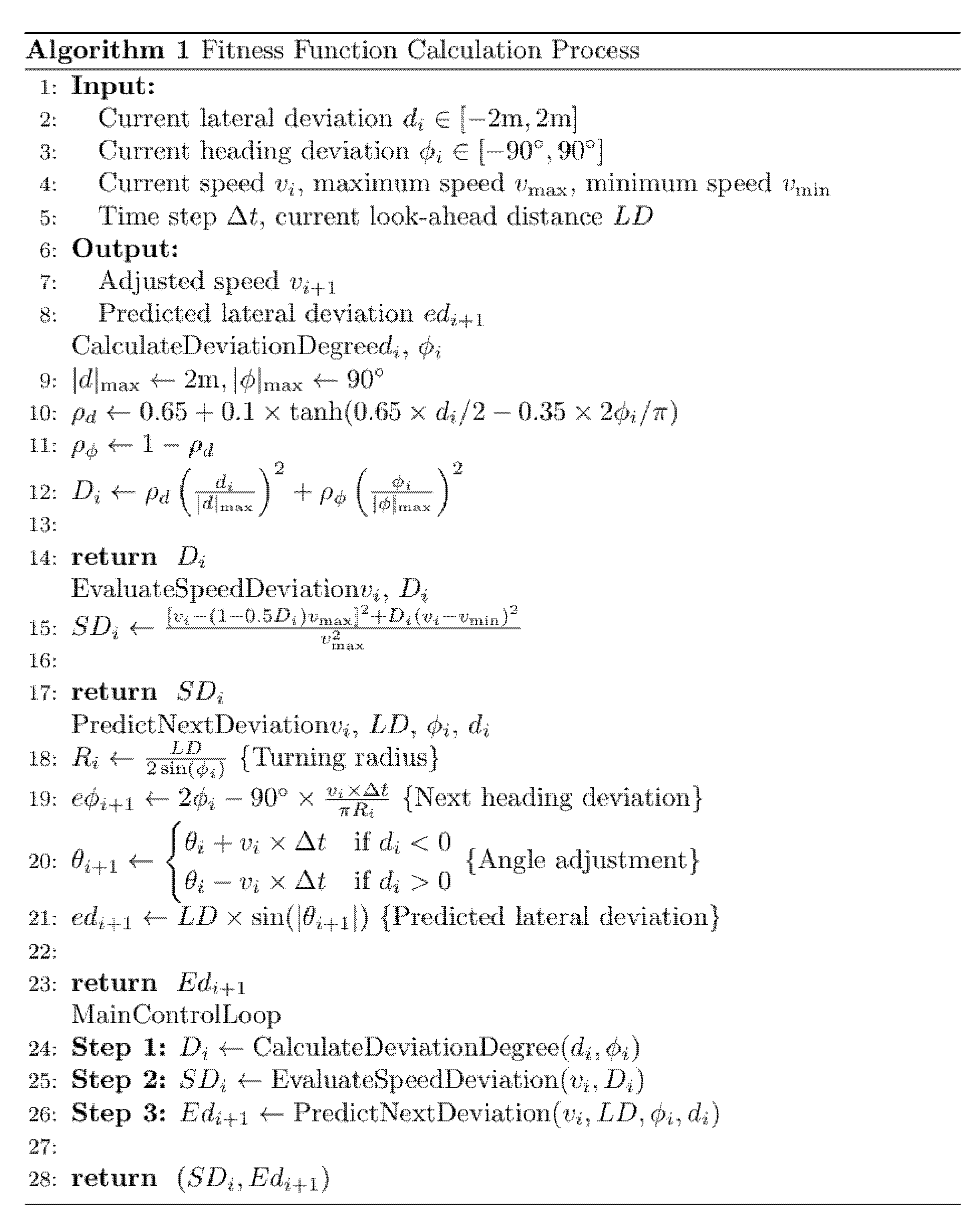
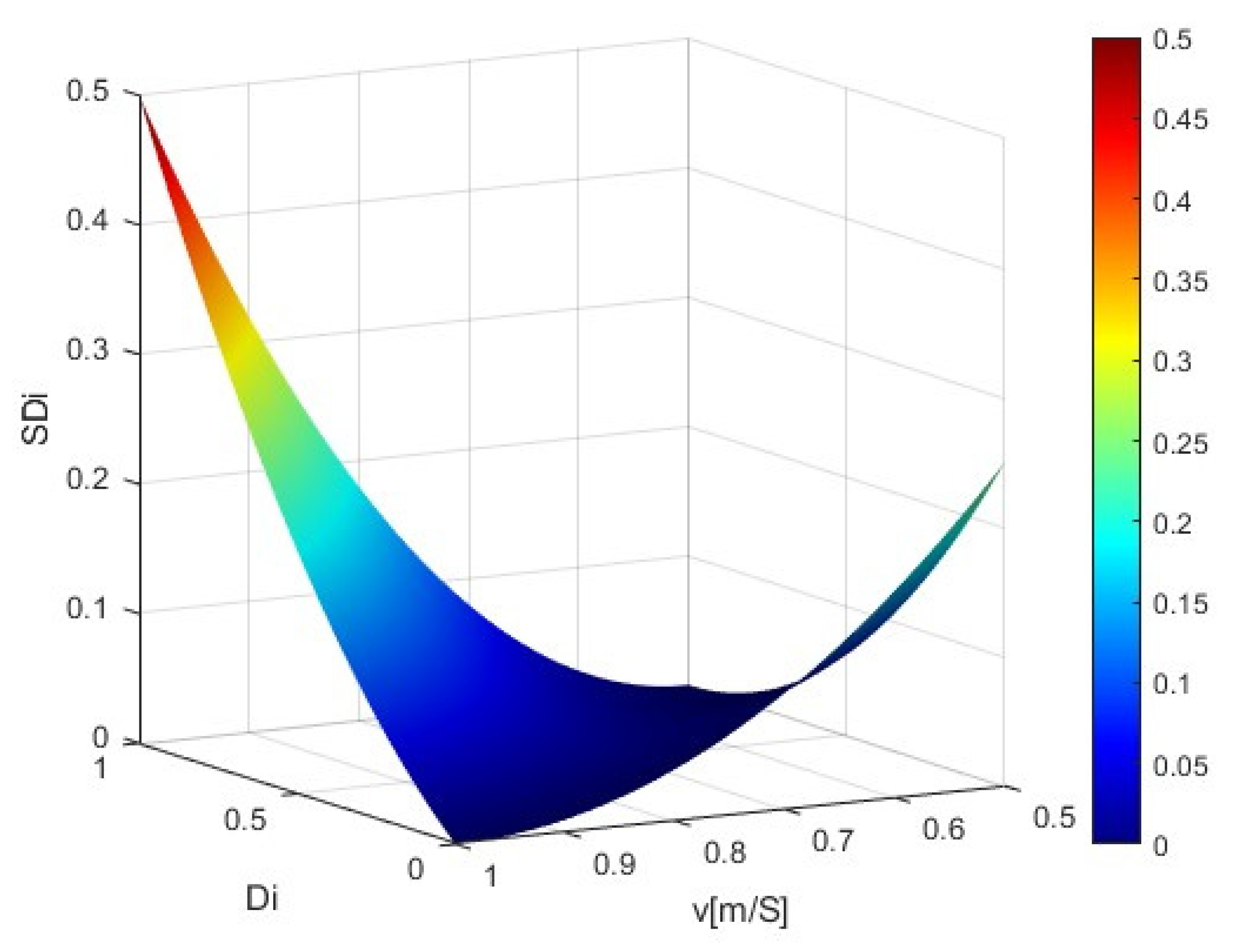
4.2. Design of the Fitness Function

The fitness function is the core of the ISSA-PP. Figure 6 shows the pseudocode of the fitness function. The fitness function constructed in this study first calculates the overall deviation (D) of the prototype using d and φ. Next, based on D, a preliminary evaluation of the current velocity is performed to obtain the speed deviation SD. Finally, using the generated velocity and its corresponding look-ahead distance, the estimated deviation (ED) of the vehicle body at the next time-step is predicted. By integrating the speed deviation and the predicted vehicle body deviation at the next time-step, the final fitness function is derived.
The steps of fitness function are as follows.
Step 1: Calculate the vehicle deviation degree (Di) at the current time (i) based on the d and φ. Based on the actual operating environment, the range for d is set to [−1 m, 1 m] and for φ is set to [−60°, 60°]. Thus, the vehicle deviation degree Di is defined as:
D i = ρ d d i d max 2 + ρ φ φ i φ max 2
In the equation, ρd is the weight of the lateral deviation, and ρφ is the weight of the heading deviation.
Considering that the d directly affects whether the prototype follows the predetermined trajectory, a slightly larger weight ρd is assigned. In this paper, the initial value for ρd is determined to be 0.65; for ρφ, it is set to 0.35. Based on the initial values, a hyperbolic tangent function is introduced to further dynamically adjust the two weights, ensuring that the value of ρd becomes more prominent when the lateral deviation increases. When the heading deviation increases, the value of ρd further decreases. The specific equation is as follows:
ρ d = 0.65 + 0.1 × tanh 0.65 × d 2 0.35 × 2 φ π
Step 2: A preliminary assessment of the current speed is conducted based on the vehicle’s deviation degree at time i, with the preliminary assessment value being the speed deviation degree SDi. The specific equation is as follows:
S D i = [ v ( 1 0.5 D i ) × v max ] 2 + D i × ( v v min ) 2 v max 2
In the equation, v is the prototype’s operating speed, vmax is its maximum operating speed, and vmin is its minimum operating speed.
[v-(1–0.5 Di) × vmax]2/v2 max ensures that the optimal value of v is vmax, specifically 1 m/s, when Di = 0. The term (1–0.5 Di) × vmax employs a linear smoothing transition, causing the optimal value of v to decrease as Di increases gradually. Di × (vvmin)2/v2 max ensures that the optimal value of v is vmin, which is 0.5 m/s when Di = 1. It also penalizes deviations of v from vmin, with the impact increasing as Di increases. The specific value of the speed deviation degree SDi in relation to the speed v and the current position deviation degree Di is illustrated in Figure 7.
Step 3: Informed by driving experience, v and LD adjust in tandem. Vehicle course correction is not just about one factor but the harmonious interplay of both. This underscores the importance of evaluating the reasonableness of speed and predicting the prototype vehicle’s expected deviation at the next moment, using the generated speed and its corresponding look-ahead distance.
Based on Figure 8 and the law of sines, the heading deviation after time Δt can be determined as follows:
e φ i + 1 = 2 φ 90 × v × Δ t π R i
the lateral deviation edi + 1 after time Δt is calculated by Equations (12) and (13):
θ i + 1 = θ i + v × Δ t d i < 0 θ i v × Δ t d i > 0
e d i + 1 = L D × sin ( θ i + 1 )
If v and its corresponding LD are determined solely based on the current body deviation degree (Di), issues like those illustrated in Figure 8 may arise. The preset path is AB. With a slightly lower speed (v1) and its corresponding LD1, the expected lateral deviation at the next moment is ((i + 1)1) is ed(i + 1)1, and the heading deviation is eφ(i + 1)1. With a slightly higher speed (v2) and its corresponding LD2, the expected lateral deviation at the next moment is ((i + 1)2) is ed(i + 1)2, and the heading deviation is eφ(i + 1)2. Although there is no significant difference in size between eφ(i + 1)2 and eφ(i + 1)1, it is evident that ed(i + 1)2 is smaller than ed(i + 1)1. Therefore, the expected body deviation degree ED(i + 1)2 at the next moment is more minor than ED(i + 1)1. At the next moment, the slightly higher speed v2 and LD2 achieve better tracking performance.
Therefore, the combined effects of v and LD should be comprehensively considered when setting the fitness function. It is necessary not only to evaluate the body deviation degree (Di) corresponding to the current speed (v), but also to predict the body deviation degree (EDi + 1) at the next moment corresponding to v and its associated LD. By integrating the speed deviation degree at the current moment (SDi) and the body deviation degree at the next moment (EDi + 1), the final fitness function (F) is defined as follows:
F = S D i + E D i + 1

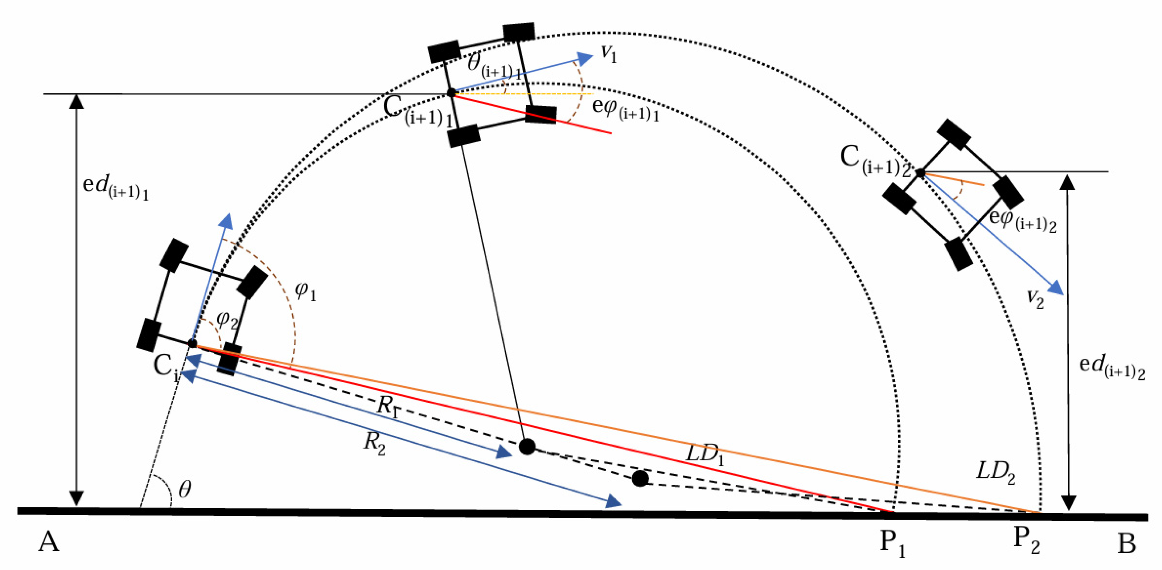
4.3. Dynamic v and LD Acquisition Process

The position of the sparrow (Xi, i = 1, 2…30) is considered the vehicle’s speed, and each speed corresponds to a specific look-ahead distance. The sparrows move within a given position range (i.e., velocity). The quality of v and LD is evaluated using the fitness function, and as v and LD continuously change, it gradually approaches an optimal value. In this paper, the steps to determine v and LD in real-time through SSA are as follows:
Step 1: Initialize the speed population by uniformly generating a speed matrix within the speed range. Then, generate the corresponding look-ahead distances using the formula for look-ahead distance given in Equation (7).
Step 2: Calculate the initial fitness value using the fitness function (Equation (14)). This involves evaluating each speed’s path-tracking performance and its corresponding LD.
Step 3: Compare the fitness values and retain the most petite individual fitness value, thereby preserving the optimal v and LD solution for the current state.
Step 4: Update each speed and its corresponding look-ahead distance, and then recalculate the individual fitness values. Compare these values to determine the global optimal solution, which represents the current optimal v and LD.
Step 5: Repeat Steps 2 to 4 until the optimal speed (voptimal) and its corresponding look-ahead distance (LDoptimal) are obtained.

5. Improved Sparrow Search Algorithm

SSA is a swarm intelligence optimization algorithm inspired by sparrow foraging and anti-predation behaviors. It is known for its strong optimization capability and fast convergence speed in the mid-term [22,23]. SSA can be applied to optimize the traveling speed and look-ahead distance during path-tracking. The traditional SSA suffers from slow convergence speeds in early stages and is prone to getting trapped in local optima. In path tracking, the optimal speed must be determined at each moment in real-time, which demands higher efficiency and accuracy in the algorithm’s solution. Improvements have been made to the traditional SSA to address this issue, as illustrated in Figure 9.

5.1. Introduction of Random Variable Tent Chaotic Mapping

As a swarm intelligence optimization algorithm, SSA exhibits significant sensitivity to initial population distributions, a characteristic that substantially impacts its search efficiency. In conventional SSA implementations, the initial population is typically generated via random sampling. However, this approach often results in uneven sparrow distribution, leading to suboptimal convergence rates during early iterations. When applied to pure pursuit path-tracking models, such randomness may delay the acquisition of optimal velocities, ultimately degrading tracking performance. To mitigate this issue, researchers commonly employ chaotic mapping techniques—primarily Tent or Logistic maps—to ensure uniform population initialization. The Logistic map exhibits the following distribution characteristics: while intermediate values are sampled with relatively uniform probability, boundary values demonstrate significantly higher occurrence frequencies [24,25]. In contrast, the Tent map provides superior uniformity across all sampling intervals but suffers from instability due to small periodic points. To address these limitations, this study introduces a modified Tent chaotic map incorporating stochastic perturbations for population initialization (Xi). This hybrid approach enhances distribution uniformity while suppressing periodic instability, thereby improving SSA’s convergence properties in path-tracking applications.
x i = 2 x i 1 + rand ( 0.5 , 1 ) × 1 popsize , 0 x α 2 ( 1 x i 1 ) + rand ( 0.5 , 1 ) × 1 popsize , α x 1
In the equation, popsize is the number of sparrows in the population, rand is a perturbation deviation factor within the range (0.5,1), and α is a scaling coefficient. The term rand (0.5,1) × (1/popsize) is the introduced random variable. This random variable maintains the randomness and regularity of the Tent chaotic map and effectively avoids issues with minor periodic points and unstable points.
To thoroughly evaluate the effectiveness of different mapping methods for initializing the population, 50 tests were conducted for each method. The average values of the distribution’s expectation and variance were calculated and are presented in Table 1.
Table 1 shows that the chaotic mapping with introduced random variables, IRV Tent, results in both expectation and variance values closer to those of a completely uniform distribution. The IRV Tent mapping effectively improves the uneven distribution of the initial population, thereby accelerating the algorithm’s convergence speed in its early stages to some extent.

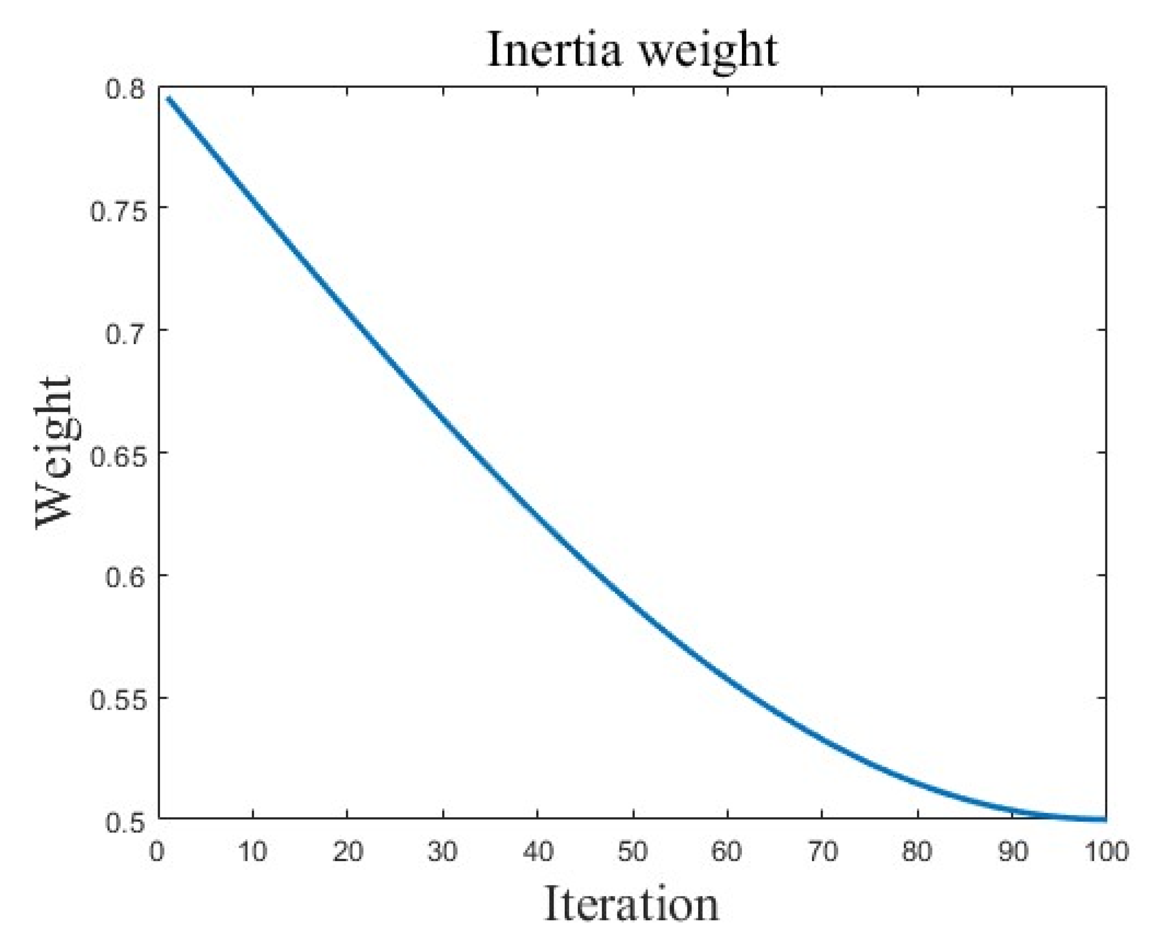
5.2. Dynamic Proportion and Inertia Weight

SSA employs a distinct population structure comprising discoverers—individuals with superior foraging capabilities—and followers, which exhibit relatively weaker food-searching abilities. Followers typically engage in localized exploration around discoverers to optimize resource acquisition. When applied to the pure pursuit model, initial velocities (v) are ranked in ascending order according to their fitness values, with the top 20% designated as discoverers. Although the roles of discoverers and followers may dynamically interchange during iterations, the conventional SSA maintains a fixed population ratio between them. This static distribution leads to a disproportionately low discoverer ratio in early iterations, constraining the algorithm’s global exploration capacity. Conversely, in later stages, an excessive proportion of discoverers impedes refined local exploitation. To address this limitation, this study introduces an adaptive role adjustment mechanism that dynamically modulates the discoverer–follower ratio. Specifically, the proportion of discoverers is increased in early iterations to enhance global search efficacy, while being progressively reduced in later phases to facilitate precise local optimization. This strategy ensures a smooth transition from broad exploration to intensive exploitation, significantly improving the algorithm’s convergence accuracy. The adaptive proportion equation is as follows:
r = 0.15 × 2 e 2 t M 0.1 rand ( 0.5 , 1 ) + 0.1
pNum = r × popsize sNum = ( 1 r ) × popsize
In the equation, pNum is the number of discoverers, sNum is the number of joiners, t is the current iteration number, M is the maximum number of iterations, and rand (0.5,1) is a perturbation deviation factor used to disturb the non-linear decrement value r.
The proportion of discoverers and joiners within the population is generated through Equations (16) and (17). As shown in Figure 10a,b, the proportion of discoverers exceeds the initially set 20% at the beginning of the iterations. As the number of iterations increases, the proportion of discoverers gradually decreases to below 20%, facilitating the transition from extensive global search in the early stages to precise local search in the later stages.
After the iteration begins, the discoverers may experience jumps during their movement towards the optimal solution. This can cause the population to converge rapidly at a single point, making the algorithm prone to falling into local optima due to overlooked search blind spots and insufficient search range. Inspired by scholars’ improvements to the inertia weight in the PSO algorithm, a perturbation strategy for the inertia weight is introduced into the SSA to update the discoverers’ positions, thereby enhancing their global search capability [26,27,28,29]. This allows sparrows with higher fitness to oscillate back and forth between different locations, improving information exchange among the sparrow population. The enhanced equation for updating the discoverers’ positions is as follows:
x i , j t + 1 = x i , j t · ω ( t ) · exp i α M , R 2 < ST x i , j t + ω ( t ) · Q · P , R 2 ST
ω ( t ) = ω max 1 sin π t 2 M + ω min sin π t 2 M
In the equation, ωmax is the maximum inertia weight, ωmin is the minimum inertia weight, x i , j t is the position of the i-th sparrow in the j-th dimension at generation t, R2 is the alarm value, ST is the safety threshold, Q is a random number following a normal distribution, P is a 1 × dim matrix of all ones, and dim is the dimension of the variables.
Equation (19) can be used to obtain the curve of ω changes with different iteration counts. As shown in Figure 11, the inertia weight decreases as the number of iterations increases.

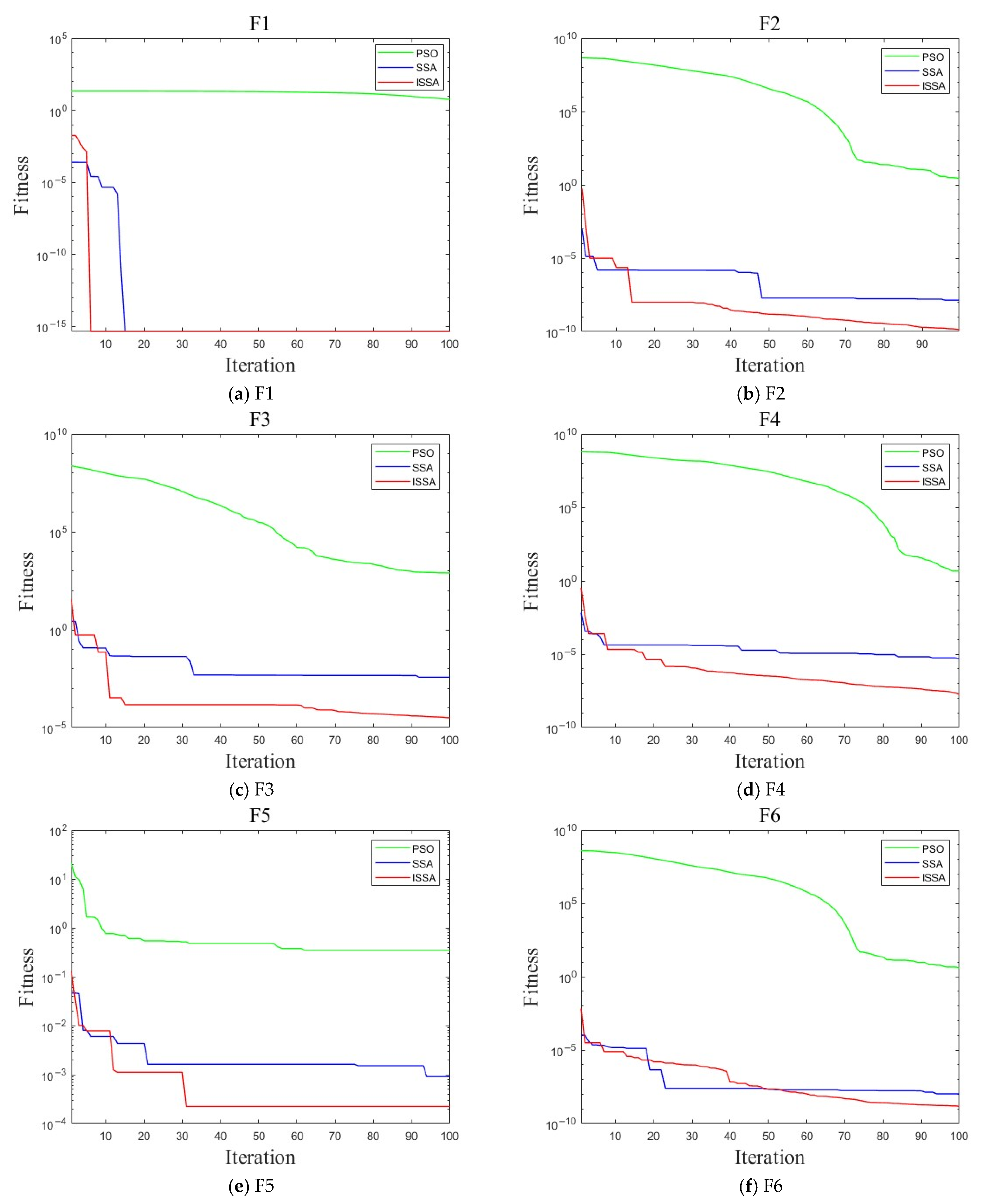
5.3. Overall Performance Simulation Test of ISSA

To comprehensively assess the performance of the ISSA, six benchmark functions were employed as fitness evaluation criteria. ISSA used in this study was compared with the traditional SSA and the Particle Swarm Optimization (PSO) algorithm. Considering the importance of achieving an optimal solution efficiently in actual vehicle tests, the maximum number of iterations for the tests conducted here was set to 100, with a population size of 30. Each test function was run 30 times. Figure 12 shows the test results of the six test functions for the three algorithms, and the resulting data are shown in Table 2
Compared to SSA and PSO, ISSA demonstrates a slight increase in optimization time for the F2 and F3 benchmarks; however, in all other performance metrics, ISSA shows significant advantages, as shown in the data in Table 2. As shown in Figure 12, ISSA exhibits a faster optimization speed in the initial stages, a smoother searching process, and better performance in escaping local extrema in the later stages to continue optimization.
From the simulation results and data of the above test functions, it is clear that the ISSA proposed in this paper effectively enhances the algorithm’s solution accuracy, efficiency, and optimization stability.

6. Experiment and Results Analysis

6.1. Experiment Design

To further verify the algorithm’s effectiveness as proposed in this paper, experimental validation was conducted in June 2024 at the Agricultural Experiment Base of Zhejiang A&F University (30.2622° N, 119.7283° E). The traditional pure pursuit model (Original-PP) and the constant speed pure pursuit model (PSO-PP), which utilizes the PSO algorithm for obtaining dynamic look-ahead distances from the existing literature, were selected as comparison algorithms. This PSO algorithm uses dynamic inertia weights to improve its convergence speed.
Field tests were conducted in a leafy vegetable cultivation environment, where the prototype performed rectangular path tracking (15 m long × 4.4 m wide) on terrain with a flatness tolerance of <3 cm. The sampling frequency was set at 10 Hz. The look-ahead distance (LD) of both ISSA-PP and PSO-PP was dynamically adjusted within [0.5 m, 1.5 m] based on tracking deviation, while a fixed LD of 1.0 m was set as a baseline. ISSA-PP employed adaptive velocity control within [0.5 m/s, 1 m/s], whereas PSO-PP and Original-PP maintained a constant speed of 0.8 m/s. All algorithms utilized a population size of 30, a maximum of 100 iterations, and a 1-dimensional search space, with identical fitness functions to ensure fair comparison.

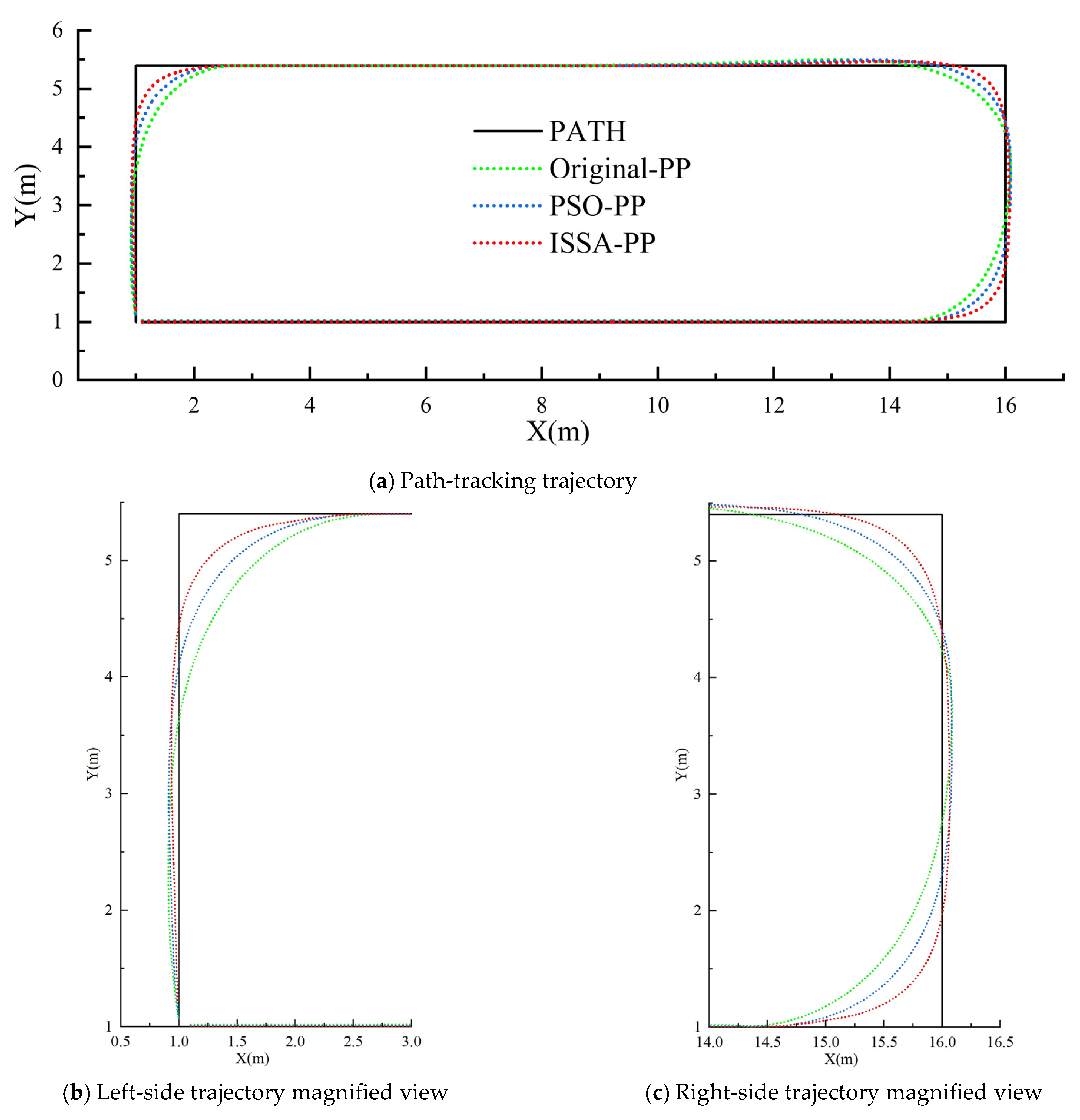
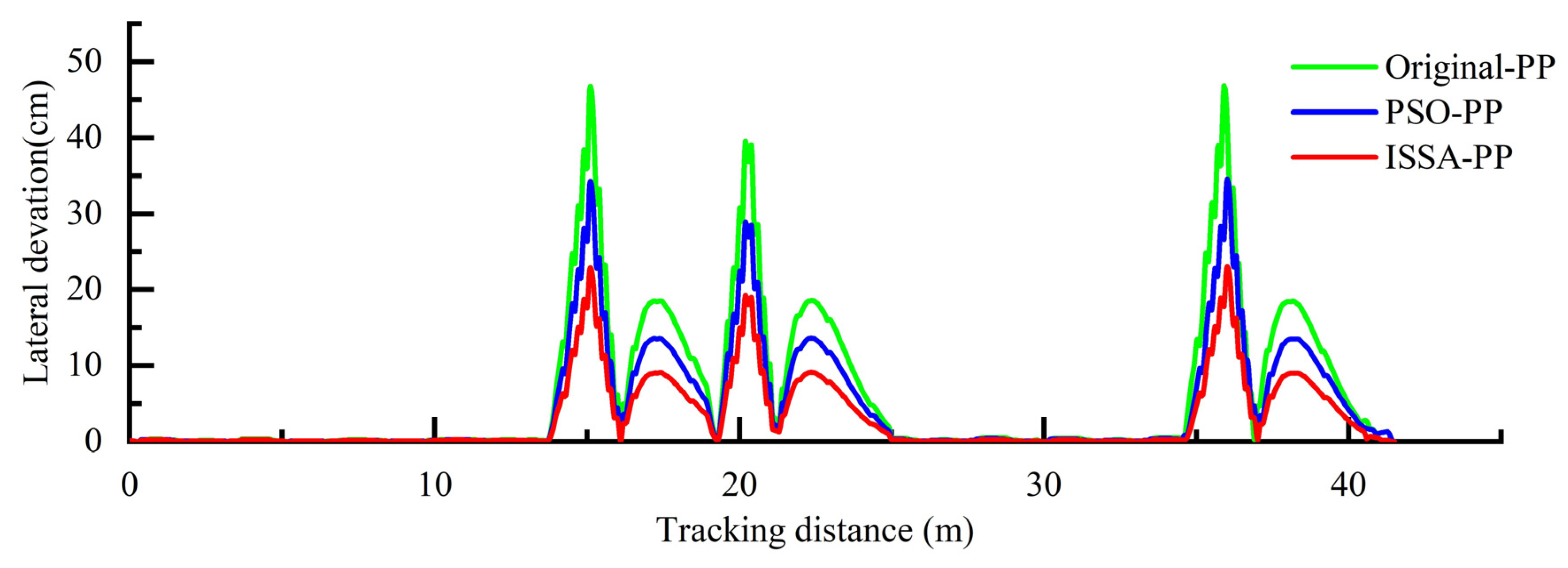
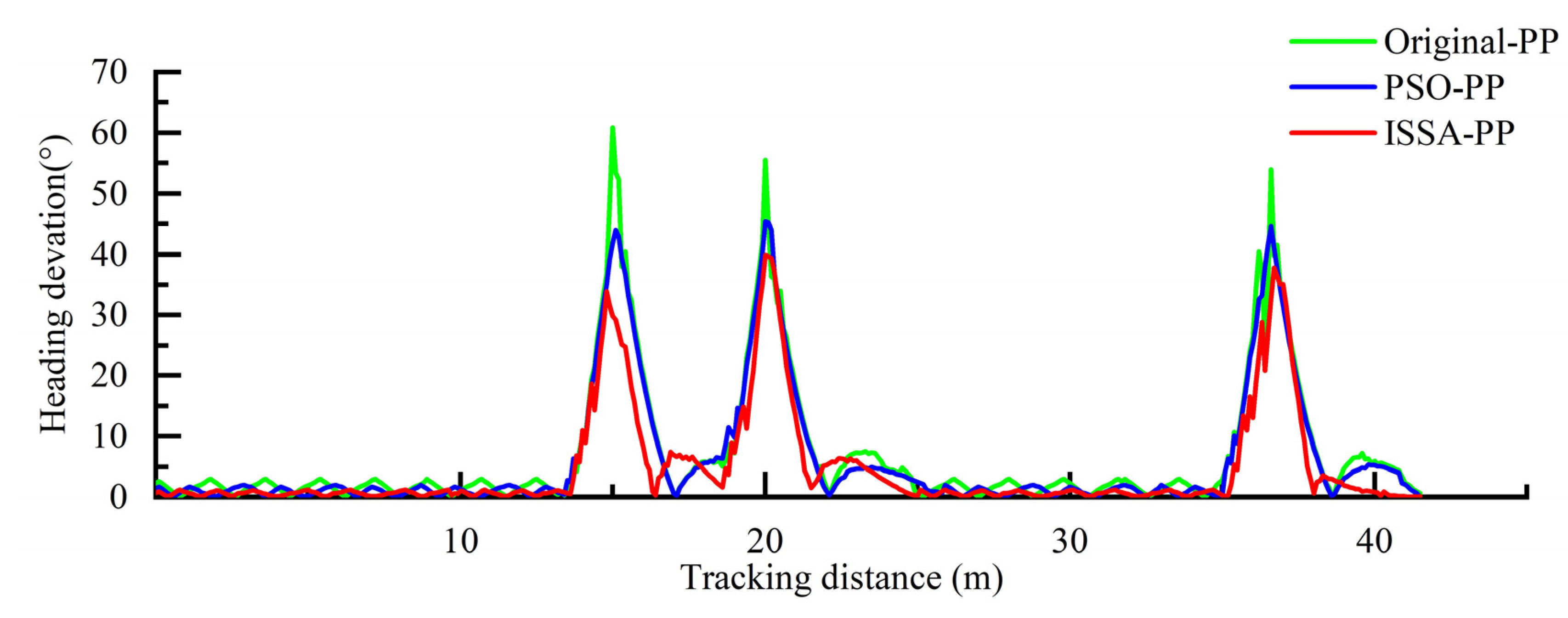
6.2. Experiment Results

Figure 13a shows the path-tracking trajectory, while Figure 13b,c, respectively, present the magnified views of the trajectories on both sides. Notably, the ISSA-PP algorithm demonstrates closer adherence to the preset path at the rectangular turns than the Original-PP and PSO-PP algorithms.
Figure 14 and Figure 15 illustrate the lateral and heading deviation variations during path tracking using three methods. Each figure illustrates the deviations.
Figure 16 illustrates the dynamic speed and look-ahead distance variation curves concerning lateral and heading deviations.
To further analyze the advantages of the proposed methods in this paper, the data obtained from Figure 14 to 16 are statistically analyzed and compiled into Table 3. The quality of path tracking is measured using the following metrics: average lateral deviation, average heading deviation, average stabilization distance, and navigation time.
To determine whether the observed differences in lateral and heading deviations resulted from random fluctuations or statistically significant effects, we conducted rigorous statistical significance tests on the experimental data. A one-way ANOVA was performed to evaluate the performance differences among ISSA-PP, PSO-PP, and Original-PP algorithms. The Shapiro–Wilk test confirmed normality (lateral deviation: W = 0.992, p = 0.052; heading deviation: W = 0.989, p = 0.102). Levene’s test assessed homogeneity of variance (lateral deviation: F = 2.42, p = 0.089; heading deviation: F = 3.15, p = 0.043). Due to violated variance homogeneity in heading deviation (p = 0.043), Welch’s ANOVA was applied. Post hoc pairwise comparisons were conducted using independent t-tests with Bonferroni correction (adjusted significance level: α = 0.0167). The comprehensive test results, as presented in Table 4 and Table 5, provide quantitative validation of the algorithm’s performance advantages.

6.3. Data Analysis

From Figure 14 and Figure 15, it can be observed that under the same planned path, the lateral deviation and heading deviation peak values of the fixed look-ahead distance pure tracking model are more significant during turning than those of the dynamic look-ahead distance pure tracking model, with a maximum lateral deviation of 46.73 cm and a maximum heading deviation of 60.91°. In the dynamic look-ahead distance model, the PSO-PP, without considering speed, has a maximum lateral deviation of 34.19 cm and a maximum heading deviation of 45.39°. When considering speed, the ISSA-PP has a maximum lateral deviation of 22.79 cm and a maximum heading deviation of 39.86°.
Figure 16 shows that the prototype’s driving speed and look-ahead distance significantly decrease as the lateral and heading deviations increase. Speed and look-ahead distance are also positively correlated.
From Table 3, it can be concluded that:
(1) The average lateral deviation and heading deviation are essential indicators of path-tracking accuracy. In three experiments, the ISSA-PP had average lateral deviations of 3.09 cm, 3.18 cm, and 3.12 cm, reducing the deviations by 33.41%, 34.30%, and 34.45%, respectively, compared to PSO-PP; it also reduced them by 51.18%, 51.52%, and 51.02% compared to Original-PP. The average heading deviations for the three experiments were 4.68°, 4.78°, and 4.92°, showing reductions of 24.64%, 26.57%, and 22.88%, respectively, compared to PSO-PP, and reductions of 31.28%, 30.52%, and 29.41% compared to Original-PP. Considering the average data from all three experiments, the average lateral deviation was reduced by 34.11% and 51.25% compared to PSO-PP and Original-PP, respectively. In contrast, the average heading deviation was reduced by 24.96% and 30.62%. This indicates that the algorithm proposed in this paper can effectively improve path accuracy.
(2) The stabilization distance refers to the horizontal distance traveled by the prototype from the start to the end of a turn, during which the lateral deviation converges to less than 5 cm. This distance reflects the speed at which the vehicle corrects its position during path tracking. In three trials, the average stabilization distances for ISSA-PP were 4.72 m, 4.53 m, and 4.87 m, which represent reductions of 31.79%, 34.16%, and 30.53% compared to PSO-PP, and reductions of 49.41%, 50.60%, and 49.31% compared to Original-PP. Based on the average data from the three trials, the average stabilization distance was reduced by 32.13% compared to PSO-PP and by 49.41% compared to Original-PP. This indicates that the proposed algorithm effectively enhances the speed of position correction.
(3) The navigation time reflects the overall efficiency of path tracking. The ISSA-PP had navigation times of 46.07 s, 47.32 s, and 45.79 s in the three experiments, which represent reductions of 12.01%, 9.85%, and 11.89% compared to PSO-PP, and reductions of 11.27%, 10.14%, and 10.64% compared to Original-PP. Considering the average data from all three experiments, the navigation time was reduced by 11.23% and 10.67% compared to PSO-PP and Original-PP, respectively. This indicates that the algorithm presented in this paper can enhance the efficiency of path tracking.
(4) As evidenced in Table 4, statistically significant differences (p < 0.001) were observed among the three algorithms regarding both lateral and heading deviations. The ISSA-PP algorithm demonstrated superior stability, exhibiting a standard deviation of 5.76 cm for lateral deviation, representing reductions of 22.62% and 48.61% compared to PSO-PP and Original-PP, respectively. Similarly, for heading deviation, ISSA-PP achieved a standard deviation of 7.60°, corresponding to 28.33% and 55.58% improvements over PSO-PP and Original-PP. The pairwise comparisons presented in Table 5 further confirmed that ISSA-PP significantly outperformed both PSO-PP and Original-PP in controlling lateral and heading deviations (p < 0.001). The 95% CI for lateral deviation between ISSA-PP and PSO-PP was [1.13, 2.11], indicating that even under the most conservative estimation, ISSA-PP still demonstrated significantly lower lateral deviation than PSO-PP. For heading deviation, the 95% CI was [0.92, 2.26], which, although slightly wider in estimation, maintained a significant lower bound. When comparing ISSA-PP with Original-PP, the 95% CI for lateral deviation was [2.66, 3.92], suggesting that in the worst-case scenario, ISSA-PP outperformed Original-PP by at least 2.66 standard deviations, demonstrating an exceptionally strong effect. Although the estimation range was somewhat broad, the extremely high lower bound reinforced the robustness of this advantage. For heading deviation, the 95% CI was [1.15, 3.07], indicating that while the improvement magnitude was less pronounced than for lateral deviation, ISSA-PP still achieved significantly superior control performance compared to Original-PP. These results collectively demonstrate that the superiority of the proposed method is not coincidental but rather stems from the inherent stability of the algorithm itself.
From the above data analysis, it can be concluded that the pure pursuit model optimized by the improved sparrow search algorithm exhibits significantly higher path-tracking accuracy and correction efficiency during turning than the original pure pursuit model and those optimized only for lateral and heading deviations.

7. Conclusions

(1) To enhance the path-tracking accuracy of agricultural machinery, this study proposes an improved pure-pursuit model incorporating dynamic v and LD, optimized via the improved sparrow search algorithm. The model determines the optimal operating speed by analyzing real-time lateral and heading deviations while accounting for the coupled relationship between velocity and look-ahead distance. Specifically, as the vehicle’s deviation increases, the system simultaneously reduces both speed and look-ahead distance to improve tracking stability. Experimental results demonstrate that the proposed method significantly outperforms conventional pure pursuit models across multiple performance metrics, confirming the efficacy of the presented approach.
(2) An improved sparrow search algorithm has been designed to address the slow convergence speed and potential local extremum issues of the original SSA in the early and late stages. This improvement involves introducing an enhanced Tent chaotic mapping for the initial population distribution, dynamically adjusting the number of discoverers, and incorporating dynamic inertia weights in the position updates. ISSA performance testing has shown that the improved algorithm significantly outperforms other algorithms in terms of solution efficiency and stability.
(3) The proposed ISSA-PP algorithm demonstrates superior performance in path-tracking control; however, several limitations should be acknowledged. The experimental validation did not comprehensively assess the algorithm’s stability under challenging field conditions, such as highly uneven terrain, dense crop occlusion, or dynamic obstacles, which may necessitate further parameter optimization in practical applications. Additionally, the tests were conducted using a small-scale vehicle platform, leaving the algorithm’s applicability to larger agricultural machinery (e.g., combine harvesters) unverified. Future research should leverage multi-sensor integration to enhance the algorithm’s environmental adaptability and compatibility with diverse agricultural machinery, thereby addressing these limitations.

Author Contributions

Conceptualization, J.W.; methodology, J.W.; validation, J.W.; formal analysis, J.W.; investigation, J.W. and L.Y. (Liwen Yao); resources, J.Z.; data curation, L.Y. (Liwen Yao); writing—original draft preparation, J.W.; writing—review and editing, L.Y. (Lijian Yao), L.X. and Z.Y.; visualization, J.W.; supervision, L.Y. (Lijian Yao), L.X., and Z.Y.; funding acquisition, L.Y. (Lijian Yao). All authors have read and agreed to the published version of the manuscript.

Funding

This research was funded by the Key R&D Program of Zhejiang (Grant No. 2022C02042, 2023C02053), the R&D Project of National Forest and Grass Machinery Sci-Tech Innovation Park (Grant No. 2023YG03) and the Research Project of Department of Education of Zhejiang Province (Grant No. Y202456233).

Institutional Review Board Statement

Not applicable.

Data Availability Statement

The data presented in this study are available on request from the corresponding author.

Conflicts of Interest

The authors declare no conflicts of interest.

References

  1. Yao, Z.; Zhao, C.; Zhang, T. Agricultural machinery automatic navigation technology. iScience 2024, 27, 108714. [Google Scholar] [CrossRef] [PubMed]
  2. Xie, B.; Jin, Y.; Faheem, M.; Gao, W.; Liu, J.; Jiang, H.; Cai, L.; Li, Y. Research progress of autonomous navigation technology for multi-agricultural scenes. Comput. Electron. Agric. 2023, 211, 107963. [Google Scholar] [CrossRef]
  3. Zhang, S.; Liu, J.; Du, Y.; Zhu, Z.; Mao, E.; Song, Z. Method on automatic navigation control of tractor based on speed adaptation. Trans. Chin. Soc. Agric. Eng. 2017, 33, 48–55. [Google Scholar]
  4. Zhang, W.; Gai, J.; Zhang, Z.; Tang, L.; Liao, Q.; Ding, Y. Double-DQN based path smoothing and tracking control method for robotic vehicle navigation. Comput. Electron. Agric. 2019, 166, 104985. [Google Scholar] [CrossRef]
  5. Li, Z.; Chen, L.; Zheng, Q.; Dou, X.; Yang, L. Control of a path following caterpillar robot based on a sliding mode variable structure algorithm. Biosyst. Eng. 2019, 186, 293–306. [Google Scholar] [CrossRef]
  6. Nguyen, P.T.T.; Yan, S.W.; Liao, J.F.; Kuo, C.H. Autonomous mobile robot navigation in sparse LiDAR feature environments. Appl. Sci. 2021, 11, 5963. [Google Scholar] [CrossRef]
  7. Liu, Z.; Zhang, Z.; Luo, X. Design of GNSS automatic navigation operation system for Leivol ZP9500 upland gap sprayer. J. Agric. Eng. 2018, 34, 15–21. [Google Scholar]
  8. Monot, N.; Moreau, X.; Benine-Neto, A.; Rizzo, A.; Aioun, F. Automated vehicle lateral guidance using multi-PID steering control and look-ahead point reference. Int. J. Veh. Auton. Syst. 2021, 16, 38–55. [Google Scholar] [CrossRef]
  9. Stano, P.; Montanaro, U.; Tavernini, D.; Tufo, M.; Fiengo, G.; Novella, L.; Sorniotti, A. Model predictive path tracking control for automated road vehicles: A review. Annu. Rev. Control 2023, 55, 194–236. [Google Scholar] [CrossRef]
  10. Hu, C.; Chen, Y.; Wang, J. Fuzzy observer-based transitional path-tracking control for autonomous vehicles. IEEE Trans. Intell. Transp. Syst. 2020, 22, 3078–3088. [Google Scholar] [CrossRef]
  11. Macenski, S.; Singh, S.; Martín, F.; Ginés, J. Regulated pure pursuit for robot path tracking. Auton. Robot. 2023, 47, 685–694. [Google Scholar] [CrossRef]
  12. Petrinec, K.; Kovacic, Z.; Marozin, A. Simulator of multi-AGV robotic industrial environments. In Proceedings of the IEEE International Conference on Industrial Technology, Maribor, Slovenia, 10–12 December 2003; Volume 2, pp. 979–983. [Google Scholar]
  13. Xu, L.; Yang, Y.; Chen, Q.; Fu, F.; Yang, B.; Yao, L. Path tracking of a 4WIS–4WID agricultural machinery based on variable look-ahead distance. Appl. Sci. 2022, 12, 8651. [Google Scholar] [CrossRef]
  14. Wu, Y.; Xie, Z.; Lu, Y. Steering wheel AGV path tracking control based on improved pure pursuit model. J. Phys. Conf. Ser. 2021, 2093, 012005. [Google Scholar] [CrossRef]
  15. Wang, R.; Li, Y.; Fan, J.; Wang, T.; Chen, X. A novel pure pursuit algorithm for autonomous vehicles based on salp swarm algorithm and velocity controller. IEEE Access 2020, 8, 166525–166540. [Google Scholar] [CrossRef]
  16. Yang, Y.; Li, Y.; Wen, X.; Zhang, G.; Ma, Q.; Cheng, S.; Qi, J.; Xu, L.; Chen, L. An optimal goal point determination algorithm for automatic navigation of agricultural machinery: Improving the tracking accuracy of the Pure Pursuit algorithm. Comput. Electron. Agric. 2022, 194, 106760. [Google Scholar] [CrossRef]
  17. Kim, S.; Lee, J.; Han, K.; Choi, S.B. Vehicle path tracking control using pure pursuit with MPC-based look-ahead distance optimization. IEEE Trans. Veh. Technol. 2023, 73, 53–66. [Google Scholar] [CrossRef]
  18. Fathy, A.; Alanazi, T.M.; Rezk, H.; Yousri, D. Optimal energy management of micro-grid using sparrow search algorithm. Energy Rep. 2021, 8, 758–773. [Google Scholar] [CrossRef]
  19. Zhao, W.; Liang, T. Optimization of terminal area arrival flight sorting based on an improved sparrow search algorithm. Sci. Prog. 2024, 107, 368504241238078. [Google Scholar] [CrossRef]
  20. Zhu, Y.; Yousefi, N. Optimal parameter identification of PEMFC stacks using adaptive sparrow search algorithm. Int. J. Hydrogen Energy 2021, 46, 9541–9552. [Google Scholar] [CrossRef]
  21. Yao, Y.; Lei, S.; Guo, Z.; Li, Y.; Ren, S.; Liu, Z.; Guan, Q.; Luo, P. Fast optimization for large scale logistics in complex urban systems using the hybrid sparrow search algorithm. Int. J. Geogr. Inf. Sci. 2023, 37, 1420–1448. [Google Scholar] [CrossRef]
  22. Xue, J.; Shen, B. A novel swarm intelligence optimization approach: Sparrow search algorithm. Syst. Sci. Control. Eng. 2020, 8, 22–34. [Google Scholar] [CrossRef]
  23. Xue, J.; Shen, B. A survey on sparrow search algorithms and their applications. Int. J. Syst. Sci. 2024, 55, 814–832. [Google Scholar] [CrossRef]
  24. May, R.M. Simple mathematical models with very complicated dynamics. Nature 1976, 261, 459–467. [Google Scholar] [CrossRef] [PubMed]
  25. Yang, B.; Liao, X. Some properties of the logistic map over the finite field and its application. Signal Process. 2018, 153, 231–242. [Google Scholar] [CrossRef]
  26. Nickabadi, A.; Ebadzadeh, M.M.; Safabakhsh, R. A novel particle swarm optimization algorithm with adaptive inertia weight. Appl. Soft Comput. 2011, 11, 3658–3670. [Google Scholar] [CrossRef]
  27. Jiao, B.; Lian, Z.; Gu, X. A dynamic inertia weight particle swarm optimization algorithm. Chaos Solitons Fractals 2008, 37, 698–705. [Google Scholar] [CrossRef]
  28. Liu, J.; Mei, Y.; Li, X. An analysis of the inertia weight parameter for binary particle swarm optimization. IEEE Trans. Evol. Comput. 2015, 20, 666–681. [Google Scholar] [CrossRef]
  29. Guo, S.; Zhang, T.; Song, Y.; Qian, F. Color feature-based object tracking through particle swarm optimization with improved inertia weight. Sensors 2018, 18, 1292. [Google Scholar] [CrossRef]
Figure 1. Physical diagram of the experimental prototype.
Agriculture 15 01215 g001
Figure 2. Schematic diagram of control system.
Agriculture 15 01215 g002
Figure 3. Diagram of the differential steering pure pursuit Model.
Agriculture 15 01215 g003
Figure 4. Schematic diagram of LD under different Kv3.
Agriculture 15 01215 g004
Figure 5. ISSA-PP algorithm flowchart.
Agriculture 15 01215 g005
Figure 6. Pseudocode of fitness function.
Agriculture 15 01215 g006
Figure 7. Current speed deviation degree graph.
Agriculture 15 01215 g007
Figure 8. Schematic diagram of deviations at the next moment for different v and LD.
Agriculture 15 01215 g008
Figure 9. Pseudocode of ISSA and the role of its improvements.
Agriculture 15 01215 g009
Figure 10. Dynamic changes.
Agriculture 15 01215 g010
Figure 11. Dynamic inertia–weight chart.
Agriculture 15 01215 g011
Figure 12. Test results.
Agriculture 15 01215 g012
Figure 13. Path-tracking trajectory and partial magnified views.
Agriculture 15 01215 g013
Figure 14. Comparison of lateral deviation.
Agriculture 15 01215 g014
Figure 15. Comparison of heading deviation.
Agriculture 15 01215 g015
Figure 16. Comparison of speed and look-ahead distance corresponding to deviations.
Agriculture 15 01215 g016
Table 1. Population distribution expectation and variance.
MethodLogisticTentIRV TentCompletely Uniform Distribution
Expectation0.75100.73560.74680.7450
Variance0.01850.01780.01970.0206
Table 2. Performance results of ISSA compared to other optimization algorithms.
Test FunctionAlgorithmBest ValueAverageOptimization Time/s
F 1 = i = 1 30 x i 2 ISSA4.45 × 10−162.95 × 10−130.056
SSA4.45 × 10−163.44 × 10−100.075
PSO1.9249.480.136
F 2 = i = 1 30 x i + i = 1 30 x i ISSA2.69 × 10−109.86 × 10−80.086
SSA1.57 × 10−68.23 × 10−60.102
PSO4.033.09 × 1070.085
F 3 = m a x i x i , 1 i 30 ISSA1.23 × 10−58.39 × 10−50.021
SSA9.36 × 10−43.09 × 10−30.033
PSO102.823.66 × 10−50.137
F 4 = i = 1 30 i j = 1 x j ISSA4.34 × 10−73.13 × 10−60.193
SSA9.36 × 10−67.75 × 10−40.244
PSO100.582.91 × 1060.377
F 5 = i = 1 29 100 x i + 1 x i 2 2 + x i 1 2 ISSA6.58 × 10−51.96 × 10−40.058
SSA7.32 × 10−48.67 × 10−40.071
PSO0.488.630.088
F 6 = i = 1 30 i × x i 4 + r a n d 0 , 1 ISSA1.09 × 10−93.65 × 10−60.058
SSA6.34 × 10−97.58 × 10−90.093
PSO71.84.05 × 1060.073
Table 3. Rectangular path tracking experimental results.
Experiment NumberEvaluation MetricsISSA-PPPSO-PPOriginal-PP
1Average Lateral Deviation/cm3.094.646.33
Average Heading Deviation/°4.686.216.81
Average Stabilization Distance/m4.726.929.33
Navigation time/s46.0752.3651.92
2Average Lateral Deviation/cm3.184.846.56
Average Heading Deviation/°4.786.516.88
Average Stabilization Distance/m4.536.889.17
Navigation time/s47.3252.4952.66
3Average Lateral Deviation/cm3.124.766.37
Average Heading Deviation/°4.926.386.97
Average Stabilization Distance/m4.877.019.43
Navigation time/s45.7951.9751.24
Average valueAverage Lateral Deviation/cm3.134.756.42
Average Heading Deviation/°4.786.376.89
Average Stabilization Distance/m4.716.949.31
Navigation time/s46.4052.2751.94
Table 4. Analysis of variance results.
Evaluation MetricsAlgorithmNMEANSDFp
Lateral Deviation/cmISSA-PP13923.135.75572.34<0.001
PSO-PP15694.757.057
Original-PP15606.4211.198
Heading Deviation/°ISSA-PP13924.787.6018.27<0.001
PSO-PP15696.3710.60
Original-PP15606.8917.10
Table 5. Independent samples t-test results.
Evaluation
Metrics
Comparison
Group
MEAN DifferenceSEtp1-βCohen’s d95% CI
Lateral Deviation
/cm
ISSA-PP vs. PSO-PP1.620.256.48<0.001>0.990.41[1.13,2.11]
ISSA-PP vs. Original-PP3.290.3210.28<0.001>0.990.83[2.66,3.92]
Heading Deviation
ISSA-PP vs. PSO-PP1.590.344.68<0.0010.980.34[0.92,2.26]
ISSA-PP vs. Original-PP2.110.494.31<0.0010.990.45[1.15,3.07]
Disclaimer/Publisher’s Note: The statements, opinions and data contained in all publications are solely those of the individual author(s) and contributor(s) and not of MDPI and/or the editor(s). MDPI and/or the editor(s) disclaim responsibility for any injury to people or property resulting from any ideas, methods, instructions or products referred to in the content.

