Article

Surface Reconstruction and Volume Calculation of Grain Pile Based on Point Cloud Information from Multiple Viewpoints

by
Lingmin Yang
1,2,
Cheng Ran
1,
Ziqing Yu
1,
Feng Han
1 and
Wenfu Wu
1,*
1
College of Biological and Agricultural Engineering, Jilin University, Changchun 130025, China
2
College of Artificial Intelligence and Manufacturing, Hechi University, Yizhou 546300, China
*
Author to whom correspondence should be addressed.
Agriculture 2025, 15(11), 1208; https://doi.org/10.3390/agriculture15111208
Submission received: 3 May 2025 / Revised: 28 May 2025 / Accepted: 30 May 2025 / Published: 31 May 2025
(This article belongs to the Section Digital Agriculture)

Abstract

Accurate estimation of grain volume in storage silos is critical for intelligent monitoring and management. However, traditional image-based methods often struggle under complex lighting conditions, resulting in incomplete surface reconstruction and reduced measurement accuracy. To address these limitations, we propose a B-spline Interpolation and Clustered Means (BICM) method, which fuses multi-view point cloud data captured by RGB-D cameras to enable robust 3D surface reconstruction and precise volume estimation. By incorporating point cloud splicing, down-sampling, clustering, and 3D B-spline interpolation, the proposed method effectively mitigates issues such as surface notches and misalignment, significantly enhancing the accuracy of grain pile volume calculations across different viewpoints and sampling resolutions. The results of this study show that a volumetric measurement error of less than 5% can be achieved using an RGB-D camera located at two orthogonal viewpoints in combination with the BICM method, and the error can be further reduced to 1.25% when using four viewpoints. In addition to providing rapid inventory assessment of grain stocks, this approach also generates accurate local maps for the autonomous navigation of grain silo robots, thereby advancing the level of intelligent management within grain storage facilities.

1. Introduction

1.1. Grain Silo Management and 3D Grain Pile Reconstruction Technologies

Grain is a strategic resource essential for national economic stability and social development. Consequently, efficient and accurate grain storage management has long been a critical area of research. Traditional methods for monitoring grain piles (primarily based on manual measurements or single-sensor systems) are often inefficient and fail to meet the real-time, high-precision requirements of modern grain logistics [1]. With recent advancements in artificial intelligence and computer vision, RGB-D cameras have emerged as a promising solution for the 3D reconstruction of grain piles. In 2020, Duysak and Yigit [2] developed a machine learning–based quantity measurement method for grain silos, highlighting early AI integration. Yariv et al. [3] proposed a neural network architecture capable of simultaneously learning unknown geometric structures, camera parameters, and a neural renderer from multi-view images for high-fidelity, high-resolution, and detail-rich 3D surface reconstruction. In 2022, Pan et al. [4] developed an optimization algorithm for high-precision RGB-D dense point cloud reconstruction in indoor settings. Lutz and Coradi [5] demonstrated IoT and AI for monitoring stored-grain quality. Xu et al. [6] introduced HRBF-Fusion, which employs Hermite radial basis functions for continuous surface representation, enhancing the accuracy of 3D reconstruction from RGB-D data. In 2023, Kurtser and Lowry [7] surveyed RGB-D datasets tailored for robotic perception in agricultural operations, highlighting their utility in grain environments. Liu et al. [8] proposed an approach combining voxels and points to improve RGB-D-based 3D reconstructions, and Vila et al. [9] implemented automatic silo-axis detection using RGB-D sensor data to monitor content levels. In 2024, Huang [10] proposed a neural distance field–based method for rapid 3D reconstruction of walnut shells, demonstrating the potential for precise volume estimation. Yu et al. [11] reviewed diverse sensors and algorithms for 3D reconstruction in smart agriculture, emphasizing their role in precision farming, and Hu et al. [12] utilized neural radiance fields for high-fidelity 3D plant reconstruction, illustrating techniques potentially transferable to grain pile contexts. Hamidpour et al. [13] applied transfer-learning techniques to achieve efficient 3D reconstructions of functionally graded materials, suggesting analogous strategies for grain. Lyu et al. [14] proposes a 3DGSR method that combines 3D Gaussian sputtering with signed distance field (SDF) to achieve efficient and high-quality 3D surface reconstruction using body rendering consistency constraints. In 2025, Kim et al. [15] proposed a deep learning-based method that estimates the volume of irregular objects by dividing the depth image into small units and predicting the volume of each unit using a neural network. Although artificial intelligence algorithms are superior in solving complex problems, they often require high hardware, arithmetic power, and algorithms, which are costly and difficult to develop. It is very interesting to develop a fast, accurate, and low-cost method for grain pile detection.
Unlike conventional RGB cameras, RGB-D devices capture both color and depth information through technologies such as structured light, time-of-flight (ToF), or stereo vision, enabling the generation of dense point cloud data. This data can be reconstructed into detailed surface models. In 2020, Miranda et al. [16] assessed data-processing algorithms for RGB-D cameras to predict fruit size and weight, demonstrating the robustness of such techniques. In 2021, Yang et al. [17] developed a high-resolution 3D reconstruction system using RGB-D data to automatically analyze crop phenotyping traits with millimeter-level accuracy. In 2022, Yang et al. [18] proposed a 3D reconstruction method for tree seedlings via point-cloud self-registration. In 2023, Wu et al. [19] demonstrated a full-utilization point cloud method to measure the angle of repose in granular materials, and Xie et al. [20] fused snapshot spectral and RGB-D images to generate 3D multispectral point clouds of plants. In 2024, Yang et al. [21] applied multi-view image reconstruction to automate plant phenotype extraction. Li et al. [22] presented an efficient 3D reconstruction and skeleton-extraction pipeline for pruning fruit trees, indicating applicability in large-scale storage monitoring. In 2024, Zhu et al. [23] further explored 3D reconstruction and volume measurement techniques for irregular objects based on RGB-D camera data. In 2025, Hu and Song [24] presented a digital image correlation calculation method for RGB-D camera multi-view matching using variable templates, improving the precision of multi-view matching. It is more commonly used in 3D shape acquisition and canopy volume calculation of plants, and its principles and methods can be applied to 3D reconstruction and volume calculation of other irregular objects.
In recent years, integrating LiDAR data with visual information has significantly advanced 3D surface reconstruction techniques. In 2024, Wei et al. [25] introduced LiDeNeRF, a method that incorporates LiDAR-derived depth priors into Neural Radiance Fields (NeRF), enhancing reconstruction accuracy in scenarios with sparse input views. Additionally, Shi et al. [26] developed a neural implicit surface reconstruction framework that jointly optimizes images and LiDAR point clouds, resulting in accurate and complete reconstructions of street scenes. These studies underscore the effectiveness of combining LiDAR data with visual inputs to improve the quality and completeness of 3D reconstructions. In 2025, Qin et al. [27] proposed a geometry-aware 3D Gaussian splatting approach that fuses dense LiDAR point clouds with imagery, achieving high-fidelity reconstructions in large-scale UAV-based applications. In these applications, LIDAR-generated point clouds are generally used for autonomous driving navigation or urban street scenes or geographic information reconstruction, where autonomous driving reconstruction point clouds are generally only identified as the type of obstacle and the distance from the center point and do not need to reconstruct the true 3D shape, while urban street reconstruction reconstructs the 3D shape but does not need to calculate the volume of the building. These point clouds are typically acquired by LiDAR on a moving vehicle or UAV. The acquisition process requires GPS-assisted localization, which is not available in the grain silo, and the robot traveling on the loose grain surface is prone to skidding, resulting in localization errors and the inability to form high-quality continuous point cloud sequences. Irregular shape 3D reconstruction requires dense point clouds, and the price of high-quality LiDAR to meet this requirement is very expensive, which affects the popularization of its implementation.
Rapid and accurate 3D reconstruction technology is crucial not only for volume estimation but also for providing navigation maps to warehouse robots tasked with operations such as leveling, inspection, and pesticide application. In 2022, Vulpi et al. [28] presented a multi-view RGB-D framework for autonomous agricultural robots. In 2024, Qi et al. [29] introduced a CNN-based loop closure detection method for RGB-D SLAM, improving robustness and real-time performance in agricultural scenarios. In 2025, Vélez [30] proposed a multipurpose UAV path-planning framework in hedgerow systems, and Vélez et al. Conti et al. [31] introduced a “ToF-Splatting” method that fuses sparse ToF depth with multi-frame integration to achieve dense SLAM reconstructions, while Storch [32] compared UAV-based LiDAR and photogrammetric systems for terrain anomaly detection—technologies relevant to large-scale silo mapping.
The 3D geometry of grain piles provides precise insights into spatial distribution, height variations, and storage density, facilitating more efficient warehouse planning and reducing dependence on manual estimation. By analyzing the reconstructed data, managers can optimize grain arrangement, enhance airflow, and prevent issues such as uneven storage or wasted space. Moreover, the integration of 3D reconstruction with inventory data enables data-driven decision-making in grain procurement by offering real-time information on storage capacity, grain quality, and stock levels. Artificial intelligence algorithms have been applied in the field of agricultural surveying, but they require high arithmetic and technical thresholds, and it is more difficult for users to modify the program.
Several international efforts have demonstrated the utility of 3D technologies in silo environments. In 2022, the Bavarian State Research Center for Agriculture (LfL) deployed a ToF camera combined with SLAM-based robotics for real-time modeling during grain intake. The system updated point clouds every 30 frames and corrected surface deviations through cloud registration, achieving an accuracy of ±2 cm, and automatically triggered alarms when a localized collapse height difference exceeding 10 cm was detected within the grain pile. However, the measurement accuracy of ToF methods declined rapidly under harsh environmental conditions, necessitating frequent sensor maintenance. In 2023, the Chengdu branch of China Grain Reserves employed a DJI M300 (SZ DJI Technology Co., Ltd., Shenzhen, China) drone equipped with a Zenmuse L1 LiDAR sensor (SZ DJI Technology Co., Ltd., Shenzhen, China) for large-scale (100,000-ton) static reconstruction, achieving a point cloud density of 500 points/m2 and a precision of ±5 cm through photogrammetric flight planning. Nevertheless, this method was unsuitable for real-time operations and encountered integration challenges with warehouse control systems. In 2021, Purdue University’s GrainCrawler robot (Purdue University, West Lafayette, IN, USA) utilized 3D reconstruction for dynamic grain leveling; however, the absence of task priority coordination led to redundancy among robots, requiring manual intervention. To address this, reinforcement learning (specifically deep Q-learning, DQN) was subsequently introduced, enabling robots to dynamically adjust task weights based on spatial variation and thereby enhancing collaborative efficiency. Meanwhile, India’s AgNext developed the FarmEye system, employing Intel RealSense D455 cameras (Intel Corporation, Santa Clara, CA, USA) mounted on a mobile scanning rig. Field tests conducted in Punjab demonstrated the system’s capability to achieve high-resolution pile reconstruction within 15 min; however, noise issues under low-feature conditions prompted the integration of infrared illumination arrays.
As shown in Figure 1, silo environments typically contain irregular grain piles with varying heights ranging from 0.3 to 1 m, with the grain surface located approximately 1.5 to 2 m below the roof structure. Leveling these surfaces is essential for ensuring long-term storage stability and operational safety. Although this task is currently performed manually, some enterprises have begun to adopt silo robots to automate the process. Consequently, accurate 3D reconstruction of grain piles is critical not only for volume estimation but also for generating navigational maps—particularly in multi-robot collaborative scenarios—thereby supporting the development of intelligent and autonomous grain storage systems. Noise issues under low-feature conditions prompted the integration of infrared illumination arrays.
In recent years, with the advancement of artificial intelligence and computer vision technologies, 3D reconstruction based on RGB-D cameras has gradually become an important approach for addressing grain pile measurement challenges. Although monocular RGB cameras can be used for 3D structure reconstruction, they require multiple measurement positions and impose higher demands on algorithms and computational power, leading to increased implementation costs. Typically, 3D structures are reconstructed by first obtaining a point cloud of the target object, followed by surface modeling. Compared with high-cost devices such as 3D laser scanners, RGB-D cameras offer advantages in terms of lightweight design and cost-effectiveness, making them particularly suitable for complex environments like grain silos. However, in practical applications, the surface morphology of grain piles is highly irregular, and point cloud data are often affected by noise, occlusions, and other environmental factors, resulting in insufficient accuracy for recognition and reconstruction. Therefore, improving the accuracy and robustness of point cloud measurements in grain silo scenarios remains a significant research challenge.
A critical aspect of 3D reconstruction for grain pile surfaces is the accurate fitting of the surface. In the context of two-dimensional data fitting, interpolation refers to estimating unknown data values from known data points. Various 2D interpolation methods are available, each suited to different applications, including linear interpolation, bilinear interpolation, spline interpolation, Lagrange interpolation, and Kriging interpolation. In 2021, Zhang et al. [33] proposed a fast linear interpolation technique that minimizes computational load. In 2022, Klančar et al. [34] combined bilinear interpolation with potential fields to navigate robots within structured environments. In 2024, Li et al. [35] developed a direct cubic B-spline interpolation for robust and accurate digital volume correlation computation. In 2022, Essanhaji and Errachid [36] presented a random algorithmic approach for multivariate Lagrange interpolation. In 2024, Supajaidee et al. [37] introduced an adaptive moving-window Kriging based on K-means clustering to improve spatial interpolation accuracy.
When selecting an appropriate 2D interpolation method, several factors must be considered, such as the nature of the data, accuracy requirements, computational resource constraints, and specific application scenarios. Different interpolation techniques possess distinct advantages and limitations, and understanding their applicability is crucial for practical implementation. For datasets exhibiting smooth variations and requiring high computational efficiency, linear or bilinear interpolation is often preferred. In contrast, when smooth transitions and higher accuracy are required, spline interpolation is generally the optimal choice. Lagrange interpolation is suitable for cases with fewer data points but a high demand for accuracy, while Kriging interpolation is more appropriate for spatial data or data with spatial autocorrelation. Thus, selecting an appropriate interpolation method requires a comprehensive evaluation of multiple factors, including accuracy, computational complexity, and the structural characteristics of the data.

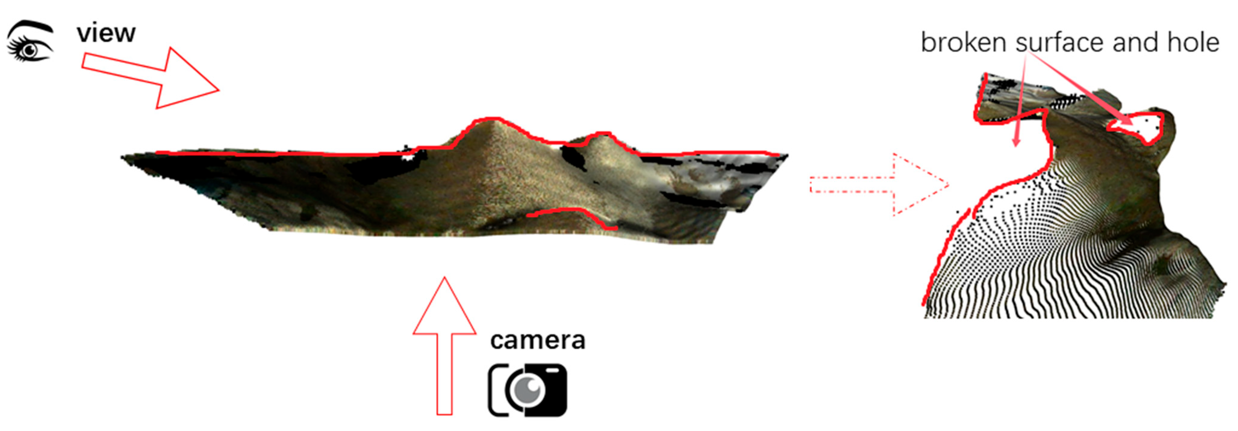
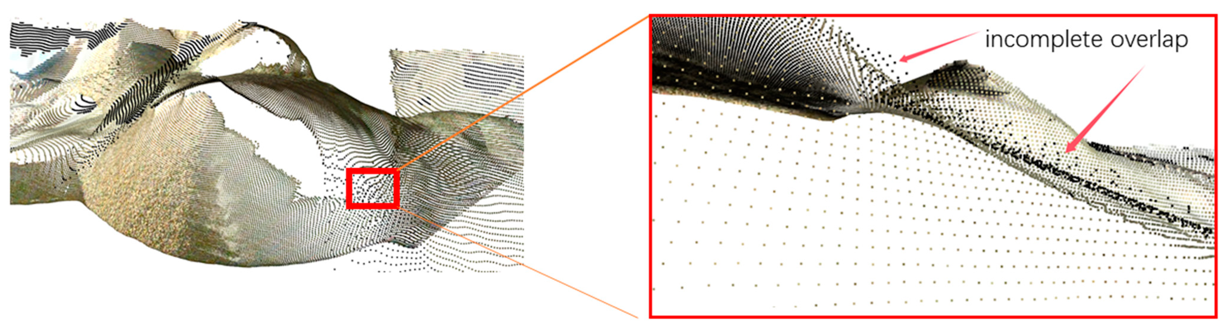
1.2. Challenges in 3D Reconstruction of Grain Piles

Complete 3D information of a grain pile cannot be obtained from a single RGB-D camera view, as the rear surfaces of the grain pile remain occluded, and occlusions between adjacent piles further exacerbate the problem. These factors often lead to defects such as discontinuities or voids in the acquired surface point cloud. To capture comprehensive 3D information, it is therefore necessary to combine images captured from multiple camera viewpoints.
Even when the camera is positioned directly above a grain pile, limitations imposed by the silo’s internal height and the camera’s field of view can prevent the capture of surface information from the far side of the pile. As illustrated in Figure 2, although the camera faces the grain pile and appears to capture its surface shape, a side view reveals that the acquired point cloud is incomplete, with missing surface details and localized voids on the rear side of the pile.
To address the limitation that a single RGB-D camera view cannot capture the complete 3D information of a grain pile, multiple camera orientations can be employed to obtain more comprehensive surface data. As illustrated in Figure 3, with an increasing number of viewpoints, the reconstructed 3D representation of the grain pile becomes progressively more complete. The surface discontinuities and gaps observed in single-view reconstructions are significantly reduced as additional camera perspectives are incorporated. If a sufficient number of viewpoints are used, it is possible to capture nearly complete 3D information of the grain pile within the field of view of the RGB-D cameras. However, while employing multiple viewpoints enhances data completeness, it also reduces measurement efficiency and introduces cumulative errors across multiple captures. Therefore, it is crucial to balance measurement efficiency and reconstruction accuracy when designing multi-view acquisition strategies.
When multiple relative orientation cameras are utilized to acquire the point cloud data of a grain pile, the resulting reconstruction does not form a perfectly continuous surface. Although the use of multiple viewpoints significantly improves the situation by providing additional information from the rear surfaces and reducing the extent of breakages and voids, noticeable defects still persist. Moreover, an important yet often overlooked issue arises in the overlap regions of different viewpoint point clouds. In these intersection areas, the combined point clouds form a denser region, but a closer inspection reveals that the surface reconstructions from different views do not fully align, as illustrated in Figure 4. This misalignment results in noticeable surface wrinkles after 3D reconstruction, which contradicts the physical reality that the surface of a grain pile—due to the natural flow of granular materials—should be continuous and smooth. Such inconsistencies in the reconstructed surface lead to inaccuracies in the calculated volume of the grain pile. Therefore, it is essential to address both the surface discontinuities (such as breakages and voids) and the misalignment issues between overlapping point clouds during reconstruction to ensure that the resulting surface is continuous, smooth, and more accurately reflects the true structure of the grain pile.

1.3. Surface Reconstruction and Volume Calculation Methods for Grain Piles

To address the challenges where a single camera viewpoint cannot capture the complete 3D structure of a grain pile and where surface reconstruction from multiple viewpoints still results in defects such as breakage, voids, and incomplete overlap in intersection areas, leading to incomplete surface reconstruction and inaccurate volume estimation, this study proposes a three-dimensional reconstruction and volume calculation method based on B-spline interpolation and clustered means (BICM) for grain pile surfaces. The proposed method resolves the issues described in Section 1.2 through the following strategies:
  • Surface continuity enhancement
To resolve the gaps and voids in the point cloud data obtained from multiple camera angles, the BICM method applies B-spline interpolation fitting. This approach eliminates surface discontinuities and produces a continuous, smooth 3D surface of the grain pile, thereby overcoming the incomplete surface reconstruction caused by defects in multi-view point clouds.
2.
Balancing measurement efficiency and accuracy
Larger sampling step sizes improve measurement efficiency and accelerate data processing but reduce the accuracy of surface reconstruction due to coarser B-spline interpolation grids. To balance measurement efficiency and reconstruction accuracy, this study systematically analyzes the relationship between different sampling step sizes and mesh interpolation step sizes on the fitted grain surface and volume estimation. Based on the analysis results, optimal parameters for B-spline interpolation are determined, achieving a balance between measurement efficiency and measurement accuracy.
3.
Correction of intersection region misalignment
To address the incomplete overlap in intersection regions formed by multiple viewpoint point clouds, the BICM method applies a clustering approach to average the points in these areas. Specifically, the relationship between five different sampling step sizes (0.1 m, 0.075 m, 0.05 m, 0.02 m, and 0.01 m) and their effects on volume estimation is analyzed. By clustering and averaging the non-overlapping regions, the method mitigates surface wrinkles caused by point cloud misalignment and reduces the influence of sampling variation, leading to an efficient and stable grain volume estimation.
The BICM method enables real-time 3D reconstruction of grain surfaces and piles within storage silos, providing crucial data for intelligent grain storage management. It also generates accurate 3D maps to support the navigation and motion planning of autonomous robots operating inside silos, promoting the application of RGB-D camera technology in the agricultural Internet of Things. In the following sections, the design of the proposed method, experimental validation, and result discussions will be detailed. surface is continuous, smooth, and more accurately reflects the true structure of the grain pile.

2. Materials and Methods

In this study, the multi-angle measurement scheme for acquiring grain pile images and point clouds was first established, and the RGB images, depth maps, and point cloud data of the grain pile surfaces were collected using an RGB-D camera. Subsequently, the YOLOv11 model was employed to detect the grain pile and determine its location within the silo. Following detection, the depth maps and point cloud data were processed through a series of operations, including cropping, merging, clustering, down-sampling, and correction. Finally, the BICM method was applied to reconstruct the surface from the 3D point cloud and to calculate the volume of the grain pile. The overall technical workflow is illustrated in Figure 5.

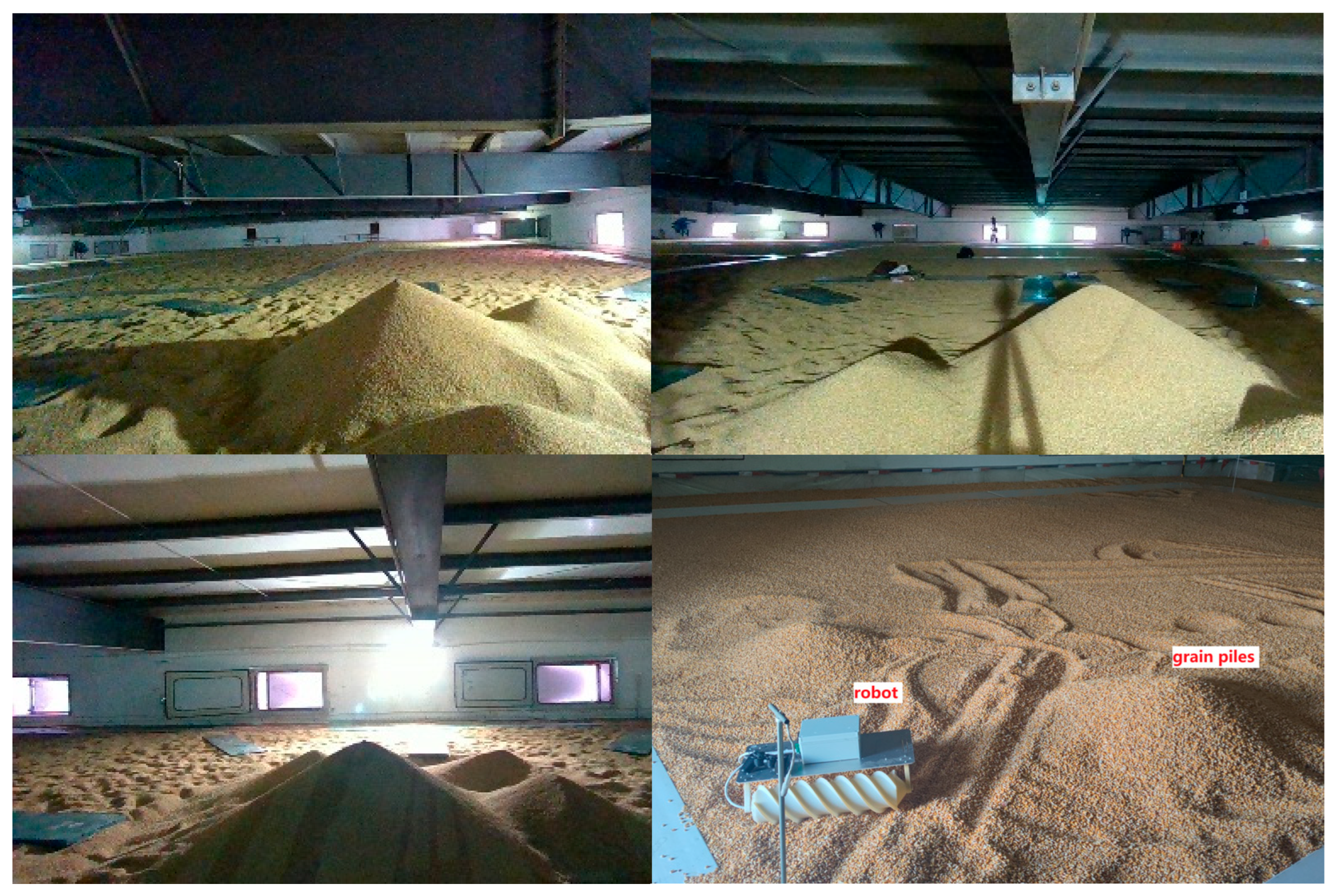
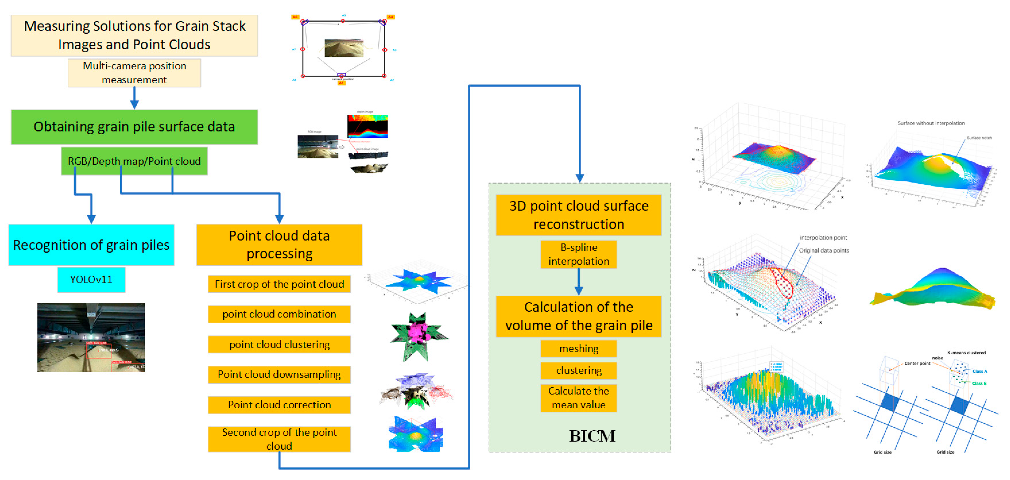
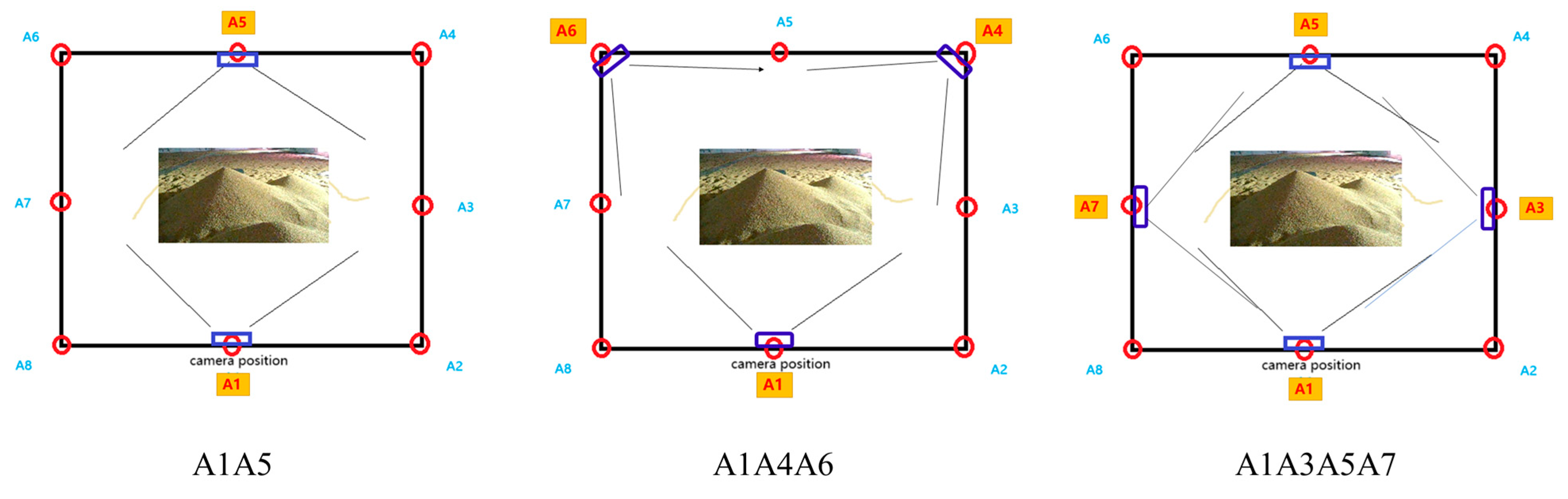
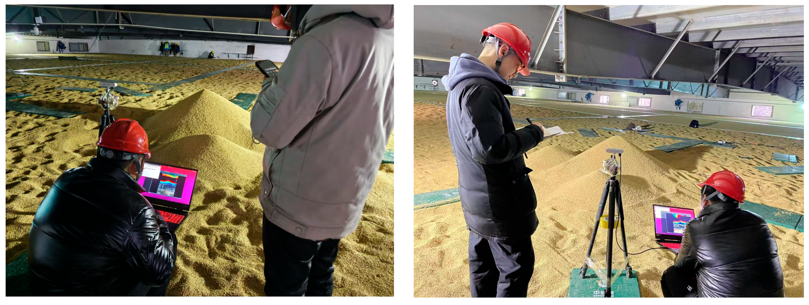
2.1. Measurement Solutions for Images and Point Clouds

The RGB-D camera used in this study to acquire point cloud data was the RealSense D455 depth-aware camera developed by Intel, designed to support computer vision and deep learning applications. This camera integrates a standard camera with an infrared (IR) sensor to provide high-quality depth images and RGB color images and is equipped with an SDK support package for development and integration.
In the grain silo, a local area was selected and designated as the measurement scene, as shown in Figure 6. Since a single camera cannot capture the information on the rear side of the grain pile, it was necessary to fuse and process point cloud data obtained from different camera locations to reconstruct the complete point cloud of the grain pile. Points A1, A2, A3, …, A8 were defined on the sides of a square with a side length of 5 m. Specifically, A1, A3, A5, and A7 correspond to the midpoints of the sides, while A2, A4, A6, and A8 represent the corners. During measurement, the RGB-D camera was placed at these points, one position at a time, at a height of 1 m and angled toward the grain pile located within the square frame. Depth point cloud data were collected sequentially from A1 to A8.
Various combinations of these measurement points were used to capture the surface information of the grain pile from different angles, including setups with two, three, four, or even eight camera positions. In addition to differences in the number of camera placements, the spatial arrangement also influenced the quality of the data. For instance, while there are 40 possible three-position combinations, configurations along the same straight line, such as A8A1A2, were less effective compared to diagonal combinations such as A1A4A6 or A2A4A6. Moreover, in practical applications, increasing the number of measurement positions does not necessarily lead to better results, as both efficiency and computational load must be considered. Therefore, a balance between measurement efficiency and accuracy must be achieved.
In this study, the two-position combination A1A5, the three-position combination A1A4A6, and the four-position combination A1A3A5A7 were selected as representative cases. The yellow background in Figure 6 highlights the camera placements and shooting angles used for comparison and analysis of their respective measurement performances. The actual measurement scene is presented in Figure 7.

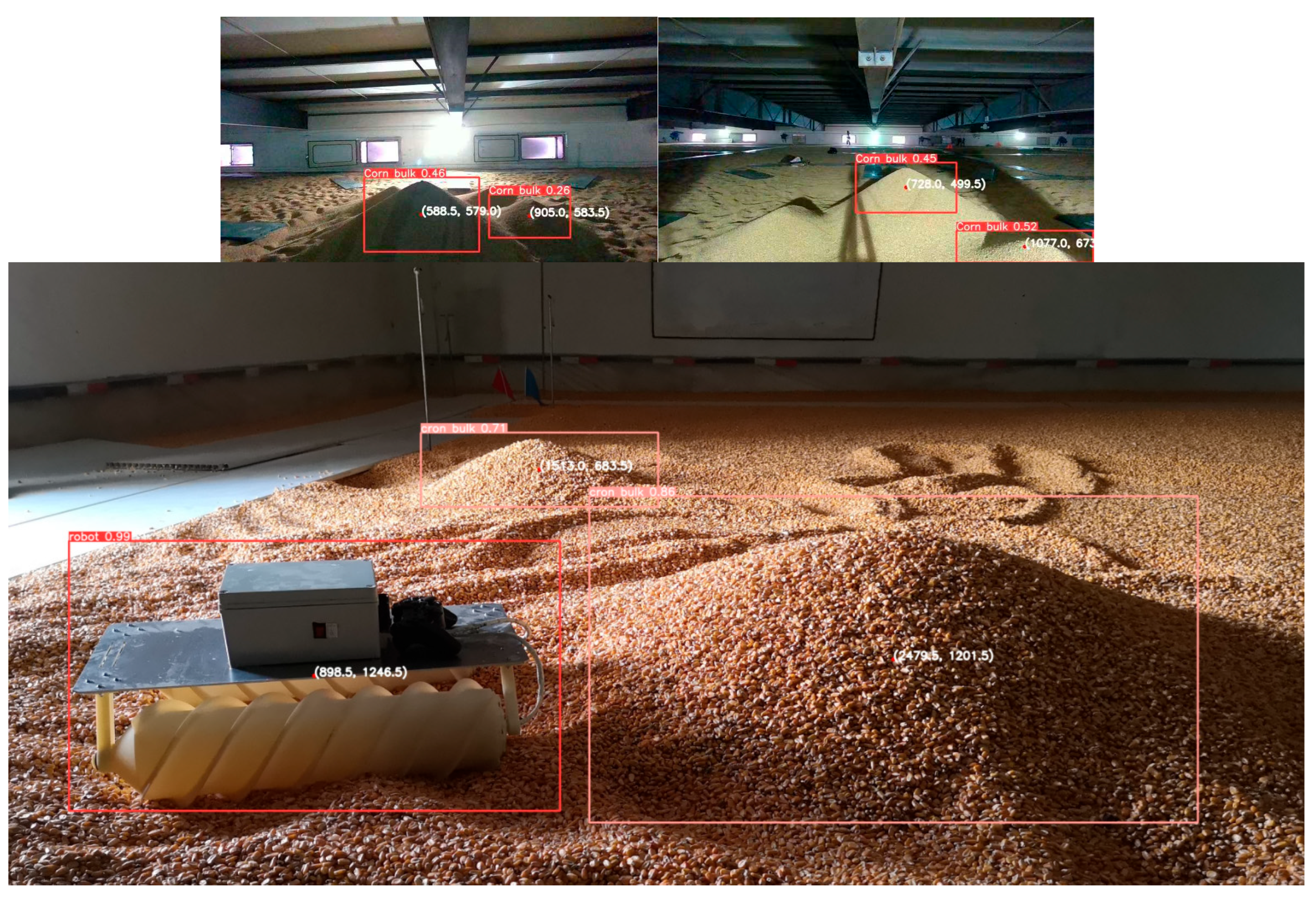
2.2. Recognition of Grain Piles

In this study, a grain pile visual detection dataset containing 1013 original images was constructed. Through data augmentation strategies such as geometric transformations (including rotation, translation, and scaling) and photometric transformations (including brightness and contrast adjustments), the dataset was expanded to a total of 64,832 images. After training a model based on the YOLOv11 target detection architecture, the grain pile recognition results are shown in Figure 8. Experimental data indicate that, under standard illumination conditions, the system achieved an average detection accuracy (mAP) of 85% for grain pile targets, while the recognition rate for the flat grain robot body reached up to 99%, with a confidence threshold set at 0.5. However, under low illumination conditions (less than 50 lux), the performance of grain pile detection degraded significantly, with the mAP dropping to a range of 26% to 45%.
It is important to note that the depth information output from the current detection system is based on a monocular visual ranging model, which calculates depth from the coordinates of the center point of the detected bounding box. There are two main limitations associated with this measurement method. First, there is a spatial deviation between the center of the detection frame and the actual geometric center of the grain pile surface, resulting in systematic errors in distance estimation. Second, data from a single frame only capture depth values at discrete points and lack the continuous spatial information necessary for a complete 3D point cloud, including the backside of the grain pile and surface normal vectors. Although this single-point ranging model can provide a rough orientation reference for the grain-leveling robot, it is insufficient for constructing critical morphological parameters such as the volume, slope angle, and curvature of the grain pile. As a result, the system cannot fully meet the demands of simultaneous localization and mapping (SLAM) algorithms, which require dense and detailed 3D environmental representations. To address these limitations, subsequent research integrates 3D vision techniques to perform surface reconstruction and enhance the completeness of spatial perception.

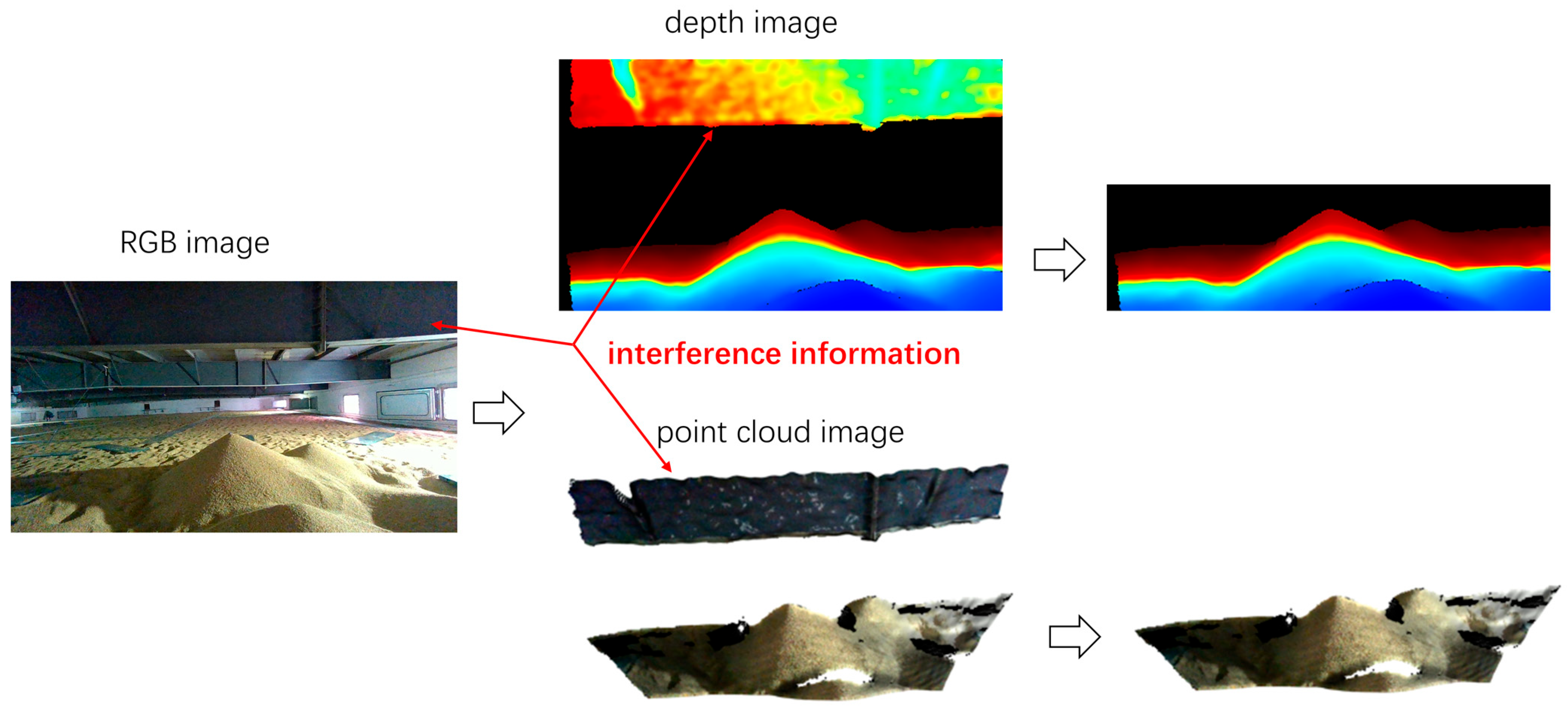
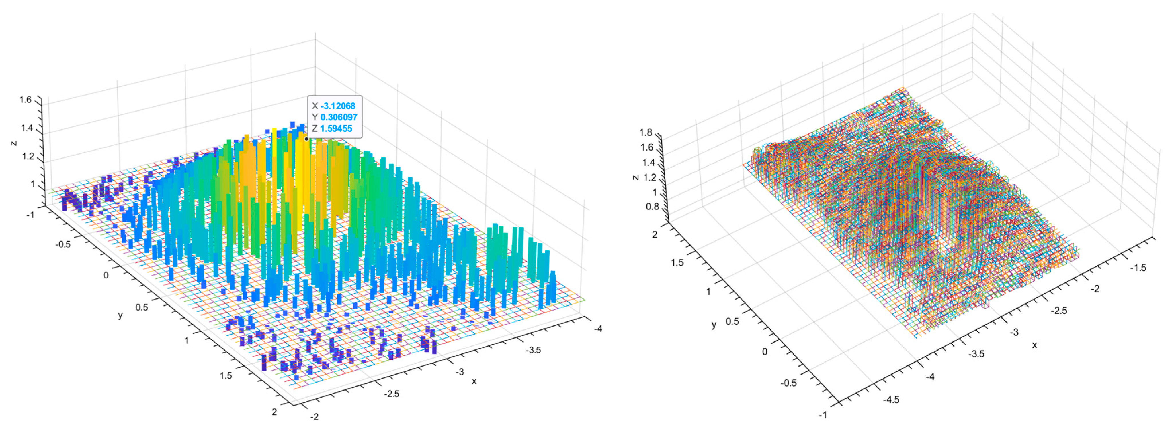
2.3. Processing of 3D Point Cloud Data

Using the RGB images, depth maps, and point clouds acquired by the Intel RealSense D455 RGB-D depth camera, the depth map records the perpendicular distance from each point on the surface of the grain pile to the imaging plane of the camera, while the point cloud provides the three-dimensional coordinates of each surface point. However, the data captured by a single RGB-D camera only represents the surface information of the grain pile from one direction, as illustrated in Figure 2, and does not include information on the backside of the grain pile. To obtain a complete 3D representation, it is therefore necessary to capture data from multiple angles to compensate for the missing information. In addition to the grain pile itself, the RGB-D camera also records other irrelevant structures within the grain silo, such as the top ceiling or partition beams. When the silo is nearly full, the grain surface can reach considerable heights, resulting in the top partition being captured in the images and point clouds. This extraneous information introduces noise that interferes with subsequent point cloud processing, as shown in Figure 9. Therefore, it is necessary to remove these interfering elements, such as internal beams and the ceiling of the silo, to ensure the accuracy of the point cloud data used for further reconstruction and analysis.

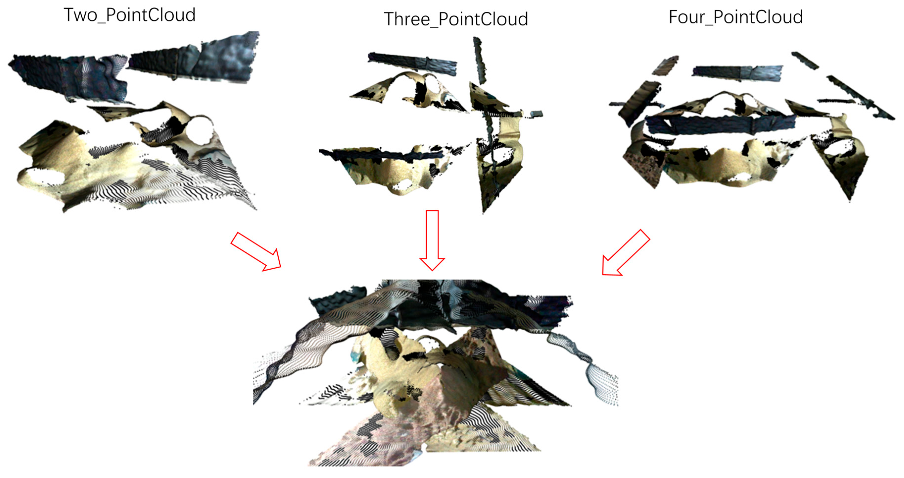
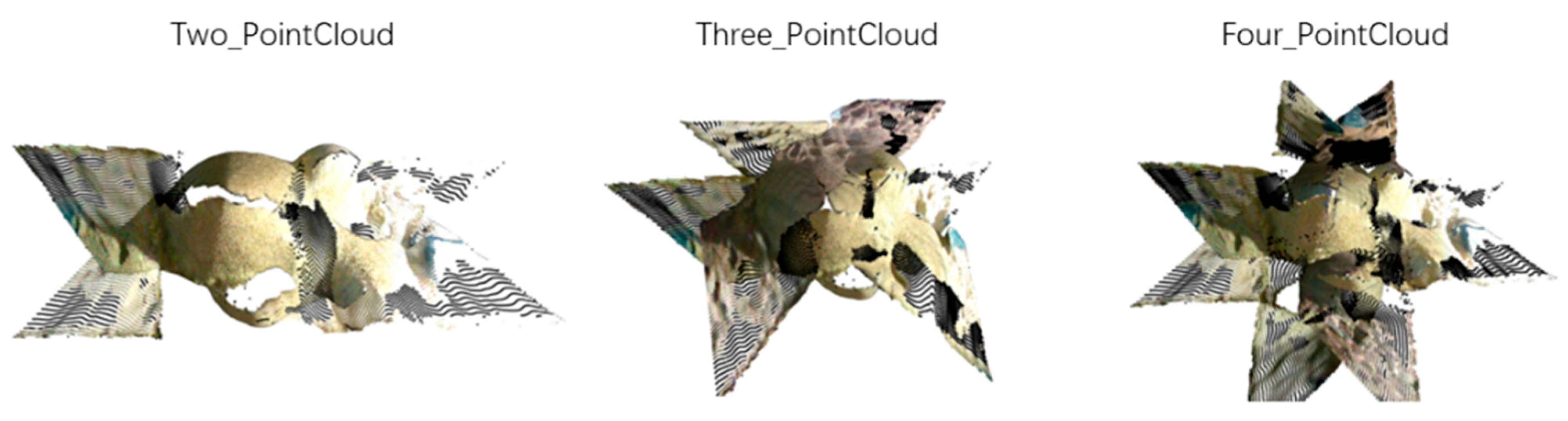
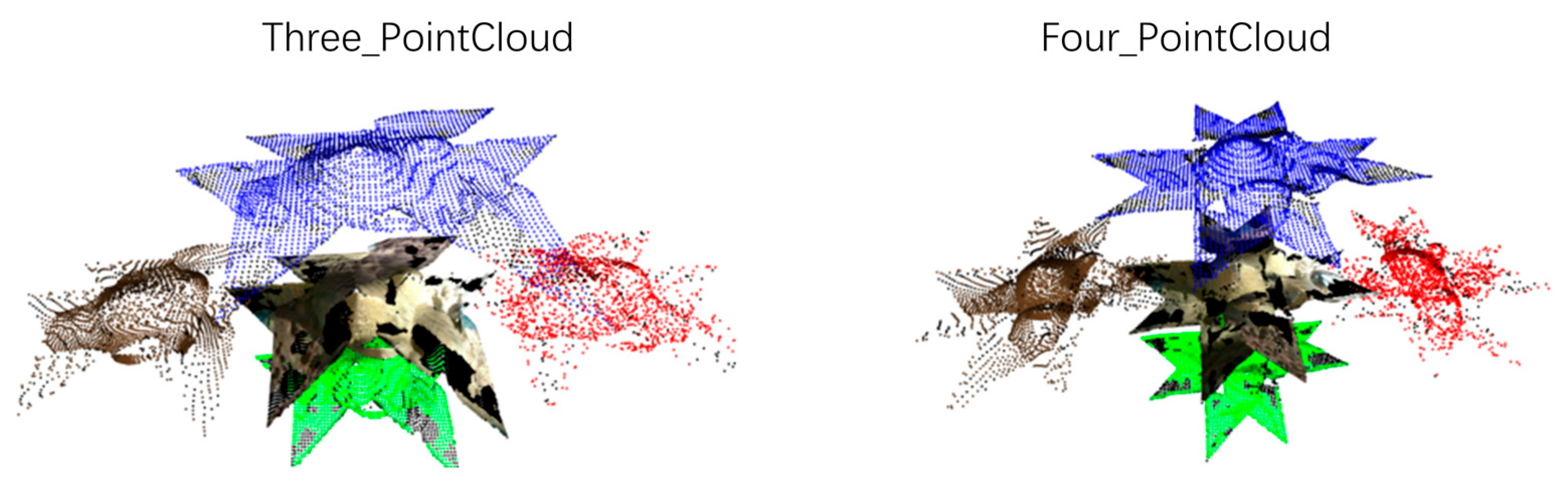
2.3.1. Multi-Angle Point Cloud Combination and Initial Cropping

When reconstructing the 3D information of the grain pile, different combinations of RGB-D camera positions can be selected. In some cases, it is possible to combine the front and back viewpoints, such as A1A5, A3A7, A2A6, and A4A8. Two positional views may not be able to obtain all the complete information of the grain pile, which depends on the camera’s field of view width. More position combinations can be used to construct more complete information about the shape of the pile; for example, three positions can be chosen from A1A4A6, A2A5A8, A3A6A8, etc., and four positions can be chosen from A1A3A5A7 and A2A4A6A8. In the same way, by using the information of the camera in these different positions, new points can be added theoretically continuously to obtain more and more comprehensive point cloud information, but this increases the measurement time as well as introduces more measurement errors. This requires balancing measurement efficiency and measurement accuracy to achieve the most reasonable solution.
When acquiring the position information of each combined point cloud, it is necessary to fuse the depth point cloud data from different viewpoints, i.e., to realize the fusion of the depth point cloud data at each position by rotating and moving the transformed matrix. In the following, two points from A1A5, three points from A1A4A6, and four points from A1A3A5A7 are fused by transformations, and the fusion of other positions is achieved in the same way. Using Open3d (v0.18), Numpy (v1.26.4), Matplotlib (v 3.9.2), OpenCV (v 4.10.0.84), and other libraries can be fused; of course, the use of MATLAB (v2024b) can also do the same thing. Detailed information regarding the matrix after applying the combined rotation and translation transformations can be found in Appendix A.
The above transformation matrix is utilized to perform the corresponding shift and rotation transformations on the point cloud to compose it into a complete 3D grain pile, and the fusion process is shown in Figure 10.
After the point cloud fusion is completed, an initial cropping of the combined point cloud is required to remove extraneous information, such as the beams at the top of the grain silo. A specific height threshold is set for cropping; in this study, a height of 1.5 m was applied to the two-point cloud combination (A1A5), the three-point cloud combination (A1A4A6), and the four-point cloud combination (A1A3A5A7). After cropping, only the grain surface information of the pile is retained, which facilitates subsequent processing. The results after cropping are shown in Figure 11, where the top baffle has been successfully removed.
It can be observed that gaps remain in the fused point clouds from different viewpoints. The two-viewpoint fusion exhibits the largest gaps, followed by the three-viewpoint fusion, while the four-viewpoint fusion results in the smallest gaps. This pattern is attributed to the increased shooting angles; as the number of viewpoints and the range of shooting angles increase, the size of the gaps in the fused point cloud is effectively reduced.

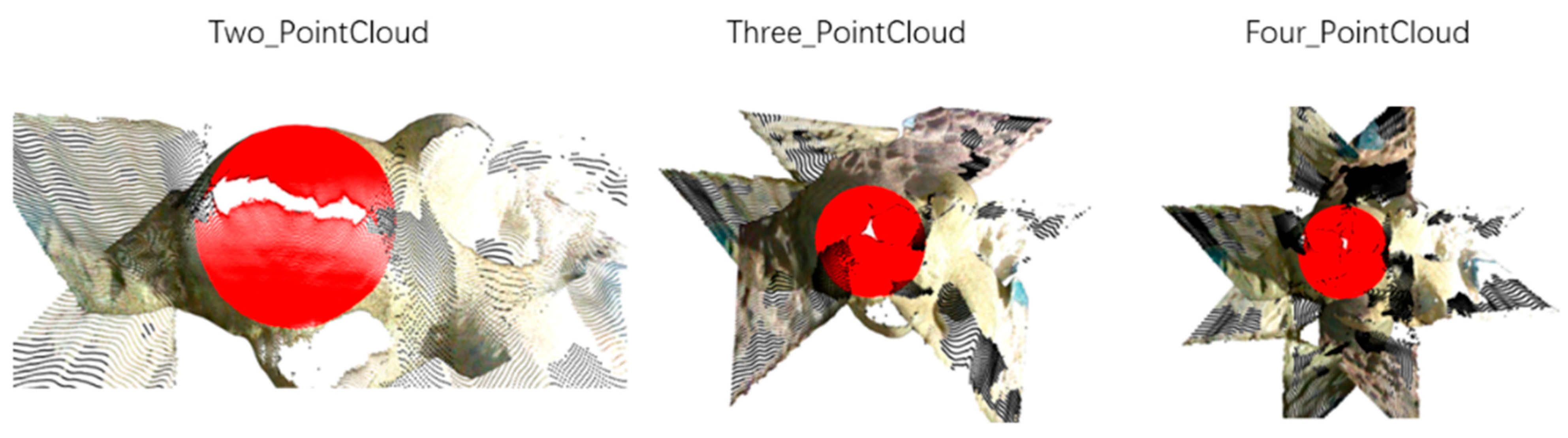
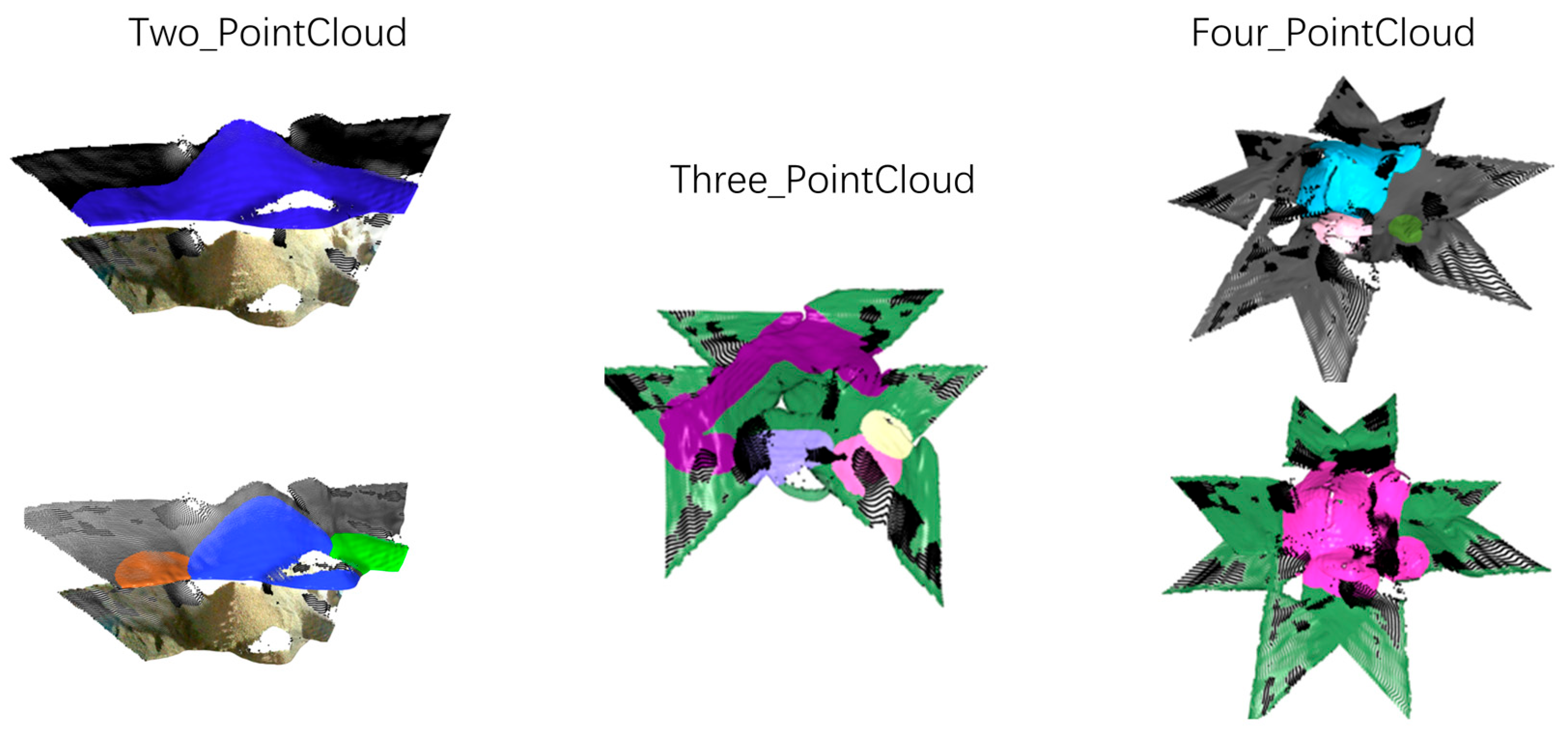
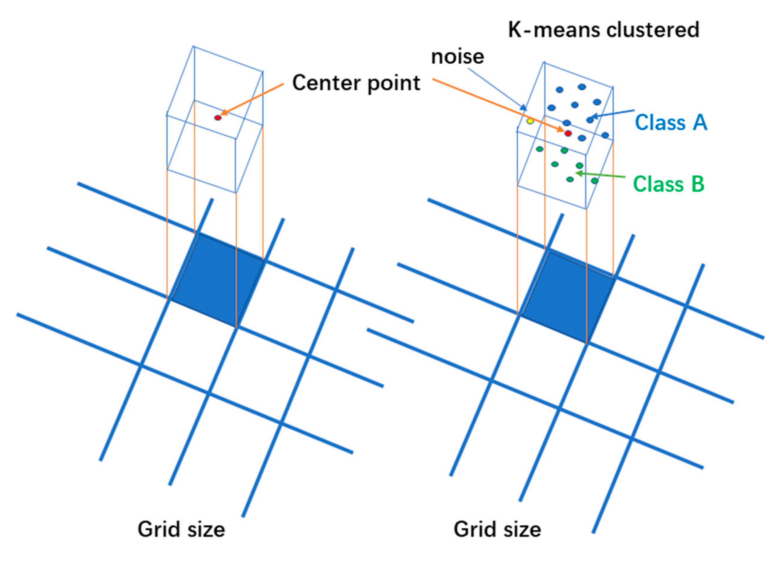
2.3.2. Combined Point Cloud Clustering

The main features of the grain pile can be extracted by applying nearest-neighbor clustering and density-based clustering to the point cloud data of the grain surface. By excluding incomplete horizontal bottom information, a more accurate 3D point cloud representation of the grain pile can be obtained, which is beneficial for subsequent volume calculation.
Using the location information of the grain pile identified by the YOLOv11 image recognition network and aligning the RGB image with the depth point cloud, the corresponding point on the point cloud can be located. From this point, the nearest N points within a specified distance are identified. The result of the point cloud clustering based on distance is shown in red in Figure 12. The center coordinates of the clustered region are (0, −0.5, −2.9), the clustering radius is set to r = 0.98 m, and points with a z-coordinate greater than 0.99 m are retained.
Density-based clustering is an algorithm that identifies clusters based on the local density of data points, enabling the detection of arbitrarily shaped clusters and the automatic filtering of noise. In this study, density-based clustering was applied to the point clouds of different grain piles, with a minimum clustering distance set to 0.285 m and a minimum number of points set to 1950. The basis for the selection of these two parameters generally relies on experience, and the main reference basis here is the density of the point cloud, which is related to the distance between the RGB-D camera and the grain pile as well as the resolution of the camera. Using this method, several distinct grain piles were identified. However, the results were highly sensitive to the choice of parameters, leading to limited stability. The clustering results are shown in Figure 13.
It should be noted that the point cloud obtained through the above clustering method exhibits a relatively large estimation error, as the depth information captured primarily represents surface points rather than points near the center of the grain pile. Nevertheless, this clustered point cloud can serve as a valuable reference for estimating the distance to the grain pile and identifying obstacle information during robot navigation within the grain silo, thereby aiding in work path planning for the grain bin robot.

2.3.3. Point Cloud Down-Sampling Processing

Due to the large volume of point cloud data, direct processing not only requires substantial storage space but also significantly increases computational costs. Therefore, point cloud down-sampling serves as an important preprocessing step, with the primary aim of reducing data size while preserving as much of the original geometric information and features as possible, thereby improving processing efficiency. Additionally, the density of collected point clouds is often non-uniform; down-sampling helps to achieve a more uniform distribution, enhancing the stability and robustness of subsequent algorithms. Common down-sampling methods include voxel grid down-sampling, random down-sampling, uniform down-sampling, curvature-based down-sampling, and farthest point sampling, each with distinct focuses suited to different application scenarios. The choice of down-sampling method involves a trade-off between efficiency and accuracy, depending on specific application requirements. For large-scale point cloud data processing, voxel grid down-sampling and random down-sampling offer fast and efficient solutions, while curvature-based down-sampling and farthest point sampling are more suitable for applications requiring feature extraction or geometric structure preservation. By employing appropriate down-sampling techniques, point cloud data can be processed and analyzed more effectively to meet the needs of different tasks.
The results of applying various down-sampling methods are shown in Figure 14. In the figure, point clouds from three and four camera positions are down-sampled: red represents random sampling, gray indicates uniform sampling, green corresponds to curvature-based down-sampling, and blue denotes voxel grid down-sampling. It can be observed that voxel grid down-sampling best preserves the structural features of the grain pile. Therefore, this study adopts voxel grid down-sampling for the initial preprocessing of point cloud data.

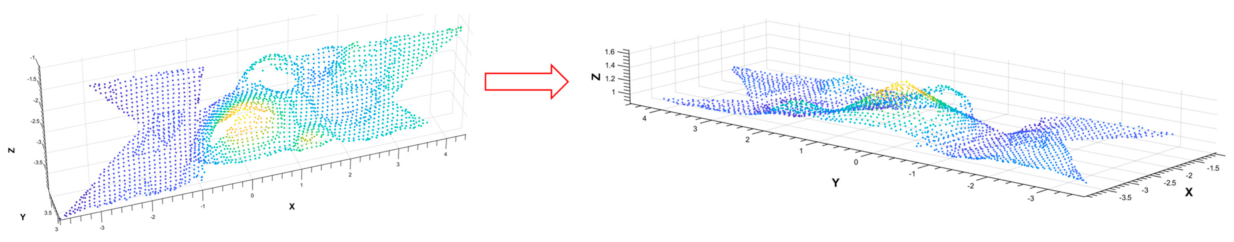
2.3.4. Correction of Point Cloud Position

During measurement, the camera is placed horizontally, resulting in the Z-axis coordinates of the point cloud acquired by the RGB-D depth camera also being horizontal. To accurately represent the actual spatial orientation, it is necessary to adjust the coordinate system so that the Z-axis aligns vertically. The effect of this adjustment is shown in Figure 15. Specifically, the adjustment involves rotating the coordinate system so that the depth direction changes from horizontal to vertical, ensuring that the Z-axis of the grain pile is oriented correctly.
Following the down-sampling processing described previously, it is observed that even when using the same down-sampling method, variations in sampling step size lead to significant differences in the density of the resulting point cloud. This disparity directly impacts subsequent point cloud fitting and volume calculation. Figure 16 illustrates point clouds obtained using sampling step sizes of 0.1 m and 0.01 m, respectively. It can be seen that the sparsity of the point clouds differs markedly; thus, the choice of sampling step size influences both the surface reconstruction accuracy of the grain pile and the precision of the subsequent volume calculations.

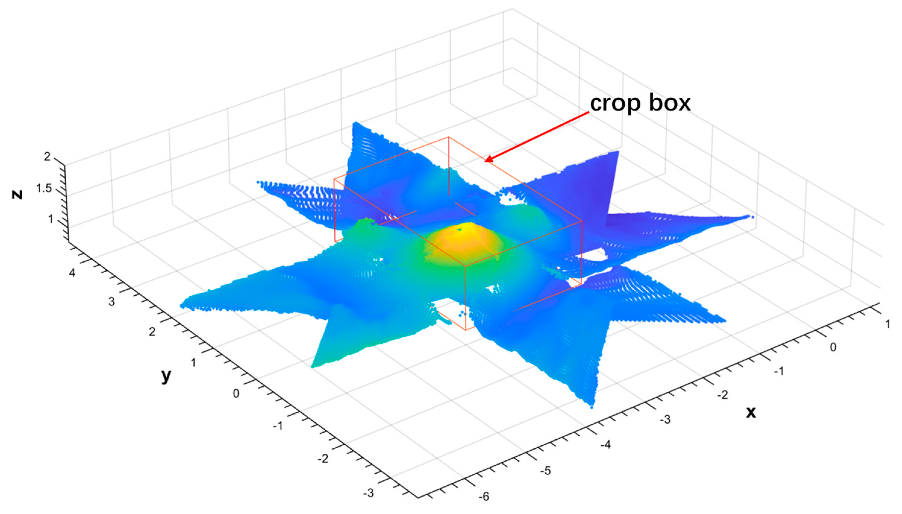
2.3.5. Second Cropping of the Point Cloud

After the down-sampling of the point cloud is completed, some grain surface information is retained when the point clouds from different angles are fused. However, the primary focus is on the information pertaining to the grain pile itself. The point clouds from two and four positions contain nearly identical grain pile information, while the grain surface information differs substantially. To facilitate comparison of the grain pile volume, a second cropping of the excess grain surface is necessary. The clipping box is indicated by the red box in the figure, with the coordinates of its lower-left corner at (−4, −2, −1) and its upper-right corner at (2, 0.5, 2.5), as shown in Figure 17.
The point cloud obtained after cropping is shown in Figure 18, where the interfering information from the grain face has been removed. It is evident that the point clouds from two, three, and four positions exhibit significant differences. The point cloud obtained from two positions has the largest gap in the grain pile, while the point cloud from three positions shows a considerably smaller gap, and the smallest gap is observed with the point cloud from four positions.
The number of points of the point cloud after the cropping of the combined point cloud at different locations is shown in Figure 19. From the first three columns, it can be observed that voxel sampling shows the most significant variation in the number of points, indicating its sensitivity to the sampling step size. In contrast, the last six columns show that radius sampling and uniform sampling are relatively insensitive to changes in the sampling step size. However, as shown in Figure 14, voxel sampling retains the features of the 3D object better. Despite its sensitivity to the sampling step size, voxel sampling proves advantageous in preserving key features. Therefore, it is essential to analyze the influence of different sampling steps on 3D surface reconstruction and volume calculation.

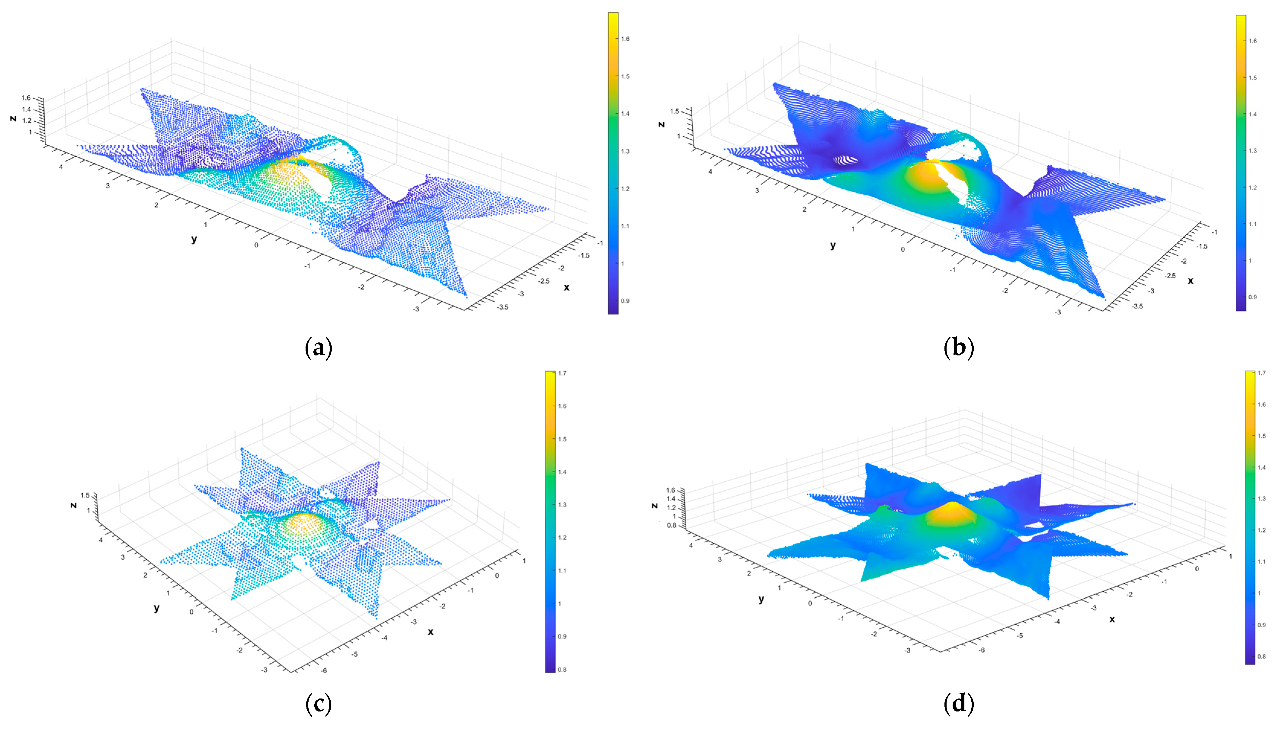
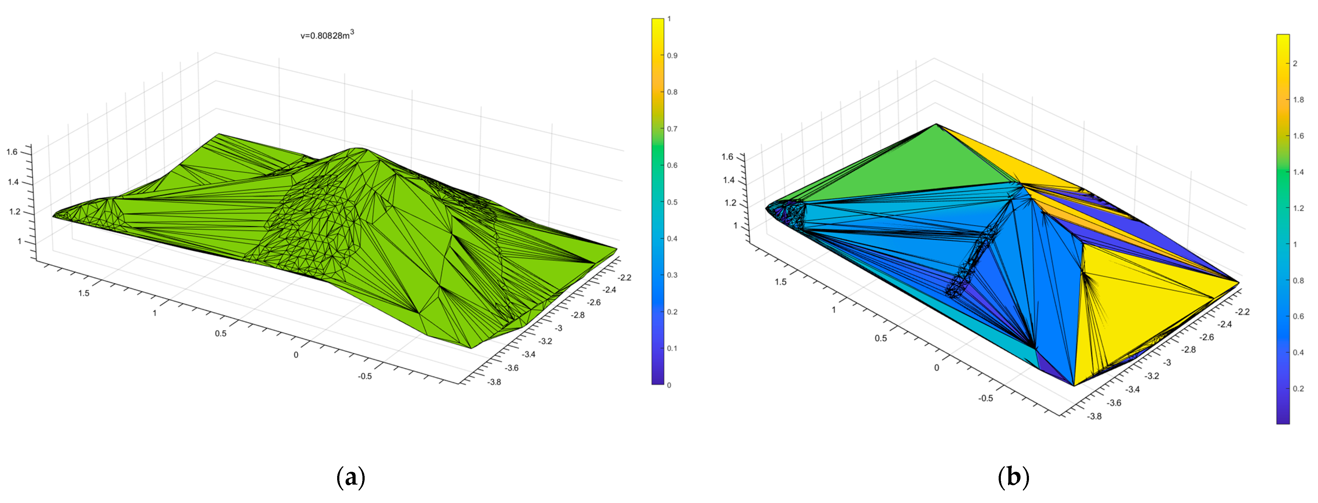
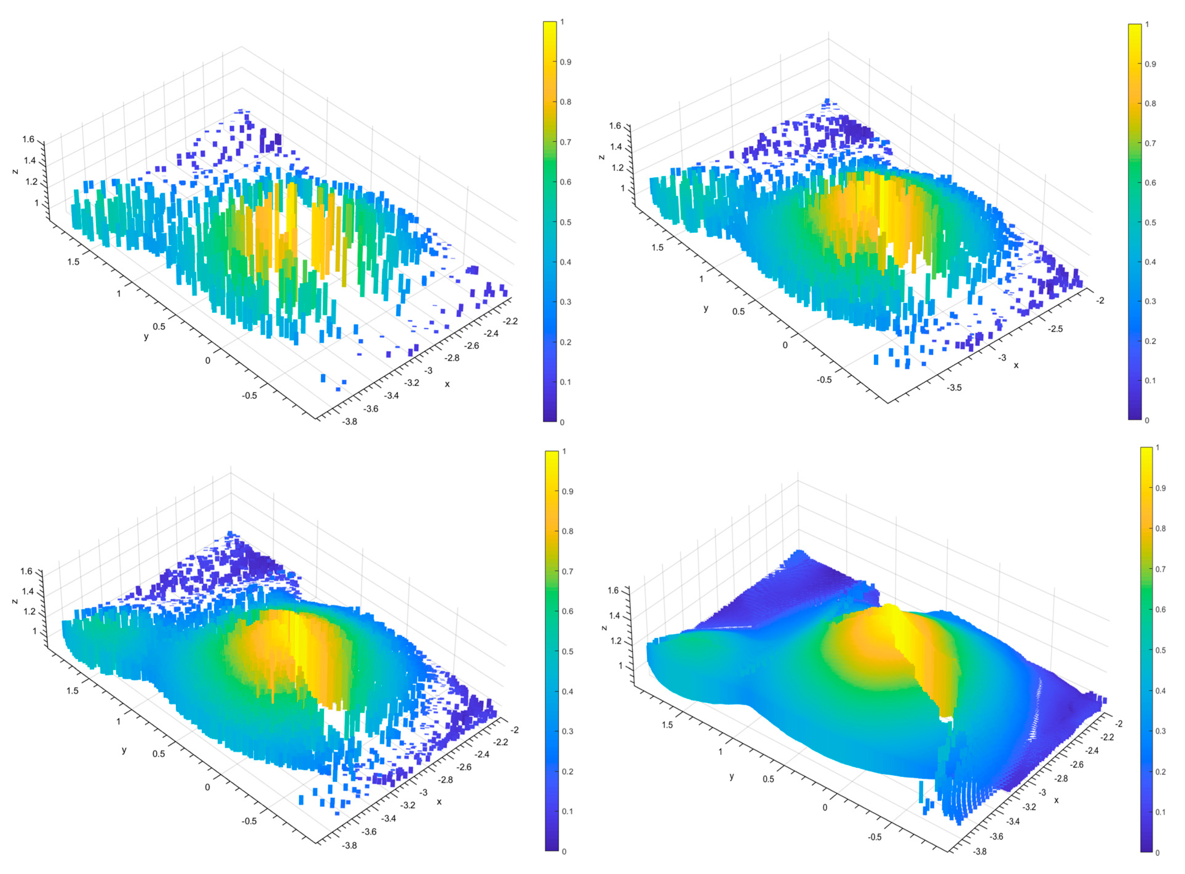
2.3.6. D Surface Reconstruction of Grain Piles

Based on the characteristics of the grain pile point cloud data in the grain silo, which ideally forms a smooth and continuous conical surface due to the self-flowing angle of the grain, a B-spline interpolation and clustered means (BICM) method for 3D reconstruction and volume calculation is proposed. This method takes into account factors such as accuracy, computational complexity, and data structure. This section first analyzes the 3D reconstruction of the grain pile surface, and the volume calculation is addressed in the following section.
Two-dimensional B-spline interpolation is commonly employed to generate smooth interpolated curves or surfaces from a given set of discrete data points (e.g., sparse point clouds, depth maps, etc.). It creates a smooth interpolation function by weighting and summing a set of discrete control points, utilizing segmented polynomials. This method has wide applications in computer graphics, data fitting, and numerical analysis, particularly when dealing with complex data. It is known for its smooth properties and computational efficiency. In the following, we will begin with 1D B-spline interpolation and progressively extend the approach to 2D B-spline interpolation.
The core of the B-spline interpolation method is the B-spline basis functions, which are segmented polynomials that guarantee the smoothness of the interpolation function. The recursive definition of the B-spline basis functions is as follows:
When the order is 0, the B-spline basis function is calculated as follows:
N i , 0 ( x ) = 1 , if   x i x < x i + 1 0 , otherwise
where is the ith basis function and is the transverse coordinate of the control point. For order p, the B-spline basis functions are computed by the following recursive formula:
N i , p ( x ) = x x i x i + p x i N i , p 1 ( x ) + x i + p + 1 x x i + p + 1 x i + 1 N i + 1 , p 1 ( x )
This formula is a linear combination of bias functions based on the previous order p-1. Given a set of control points x_i ,   f x_i   , the 1D B-spline interpolation function is as follows:
S ( x ) = i = 1 n N i , p ( x ) f ( x i )
where f ( x i ) is the known function value at the control point, N i , p ( x ) is the ith B-spline basis function of order p, and S ( x ) is the interpolation result.
Two-dimensional B-spline interpolation has the same basic idea as 1D B-spline interpolation. The difference is that 2D B-spline interpolation takes into account two directions: the x-direction and the y-direction. To make the interpolation function smooth, the key to 2D B-spline interpolation is to use the B-spline basis function for each of the two directions. Given a set of 2D control points { ( x i , y i , f ( x i , y i ) ) } , 2D B-spline interpolation can be performed by using B-spline basis functions for the x and y directions separately. The interpolation function for 2D B-spline interpolation can be expressed as follows:
S ( x , y ) = i = 1 m j = 1 n N i , p ( x ) N j , q ( y ) f ( x i , y j )
  • f ( x i , y j ) is a known function value at the grid point ( x i , y i ) ;
  • N i , p ( x ) is the ith B-spline basis function in the x direction of order p;
  • N j , q ( y ) is the jth B-spline basis function in the y direction of order q.
The 2D B-spline basis function is defined by using the product of the B-spline basis functions in the x-direction and y-direction, respectively, i.e., the 2D B-spline basis function is defined by expanding the one-dimensional B-spline basis function in both directions. In the x direction, the basis function N i , p ( x ) is recursively defined as follows:
N i , p ( x ) = x x i x i + p x i N i , p 1 ( x ) + x i + p + 1 x x i + p + 1 x i + 1 N i + 1 , p 1 ( x )
In the y direction, the basis function N j , q ( y ) is recursively defined as follows:
N j , q ( y ) = y y j y j + q y j N j , q 1 ( y ) + y j + q + 1 y y j + q + 1 y j + 1 N j + 1 , q 1 ( y )
The 2D B-spline interpolation is computed by first interpolating in the x-direction, written as follows:
f ( x , y ) = i = 1 m N i , p ( x ) f ( x i , y )
Then interpolate in the y-direction, written as follows:
S ( x , y ) = j = 1 n N j , q ( y ) i = 1 m N i , p ( x ) f ( x i , y j )
With this formula, we can utilize the smoothness and continuity of the B-spline interpolation function to calculate the interpolation value of any point x. The fitted surface of the point cloud is shown in Figure 20. It can be seen that the red points in the figure are the original data points, and the blue points with red edges are the data points generated by the interpolation and fitting of the BICM method. It is evident that the BICM method effectively fills the surface of the grain pile with the grid of the notch and the void portion at a certain step size, resulting in a continuous and smooth fitted surface of the grain pile.
The piecewise point cloud reconstructed by the Poisson method is shown in Figure 21, and it needs to determine the depth information of the octree of the point cloud, but the adjustment of the parameters is more complex and inflexible. As can be seen in Figure 21 and Figure 22, the reconstruction of the 3D surface of the grain pile is only the surface information of the surface, and the volume information of the grain pile cannot be obtained directly, and the calculation of the volume of the grain pile needs further processing.

2.4. Volume Calculation of the Grain Pile

If the surface points obtained without interpolation will have obvious gaps, as shown in Figure 20, and the step size of the mesh will affect the size of the volume, such as too large will cause the calculated volume to be too large, while too small will make the calculated volume small due to too many gaps.
When using the Alpha surface fitting method to directly calculate the grain pile volume, as shown in Figure 23a, the resulting surface is incomplete and contains small discontinuities. Alternatively, if the volume is calculated based on the spatial convex hull formed by the convex enclosure of the Delaunay triangulation (Delaunay_convhull), as shown in Figure 23b, many flat surfaces are generated, leading to a poor fit to the true shape of the grain pile. However, because this method neglects detailed surface variations, the calculated volume is less accurate but more stable. The results of these two direct surface reconstruction approaches for volume estimation are presented in Figure 23.
After obtaining the 3D surface, the volume beneath it must be calculated. If the surface equation were known, the volume could be obtained via double integration. However, since the grain pile surface is represented by point cloud data collected using an RGB-D depth camera and its explicit surface equation is unknown, alternative methods must be employed. The gridded product method and Simpson’s rule are two commonly used numerical integration techniques for volume estimation. Their main purpose is to approximate the integral by discretizing the region into small blocks and approximating the product function within these blocks.
Let R be the region of integration and be the function to be integrated. Discretize the region R into an m × n grid with each grid cell of size. And, where [ a x , b x ] and [ a y , b y ] are the integration intervals of x and y, respectively, and hence the volume of integration can be approximated as follows:
V i = 0 m 1 j = 0 n 1 f ( x i , y j ) Δ x Δ y
where are the equivalent height coordinates of the mesh nodes? Because the point cloud aligned together may contain multiple points in the same grid interval, the general practice is to take the maximum value of all the points in this grid as the height of the grid and accumulate the volume of all the columns to finally obtain the volume of the final object to be measured, as shown in Figure 24.
The idea of this method is simple and direct, but the accuracy is often not high enough when there is noisy data in the point cloud. This study proposes to use the density clustering averaging method, i.e., the key idea of clustering is that if there are enough points in the neighborhood of a point, then these points are considered to be a part of a cluster, and by clustering and then weighting the averaging method or obtaining the equivalent height value in the grid, thus eliminating the effect of noisy data, and density clustering does not require clusters to be spherical but can handle clusters of arbitrary shape.
Clusters are defined based on two main parameters: the neighborhood radius ϵ defines the range of a point’s neighborhood, and the minimum number of points defines the minimum number of points that a point needs to contain within ϵ’s neighborhood to be used as the core point of a cluster. Let there be a set of points where each point has an ϵ-neighborhood, and a point’s ϵ-neighborhood is the set of all points whose distance from P is less than ϵ, denoted. And it is a core point if and only if, the following is valid:
| N ϵ ( P i ) | M i n P t s
Here, ϵ M i n P t s and are sensitive parameters, but because the surface of the ideal grain pile is continuous, it can be easily controlled here by setting ϵ to 0.05 m and M i n P t s to 200. Then we need to consider the number of clusters of clustering. Again, because the surface of the ideal grain pile is continuous, the number of clusters cannot be too many. Taking into account the existence of the measurement error, the maximum allowable number of clusters is 2. When the amount of clustering exceeds 2, then it means that there is a large noise point that should be resampled. When the density clustering of the cluster meets the requirements the mean value should be sampled instead of the maximum height. If there are n clusters of cluster C and there are | C | points, each point of the Z coordinates were then the clustering of the Z coordinates of the mean (center of gravity) and are calculated as follows:
centroid Z = 1 n * | C | i = 1 | C | Z i
Algorithm 1 for the clustered mean method is as follows:
Algorithm 1: CM(D, ε, MinPts)
        1. Initialize all points as unvisited.
        2. Create an empty list clusters[] to store clusters.
        3. For each point p in D:
                a. If p is unvisited:
                        i. Mark p as visited.
                        ii. Find all points in N_ε(p).
                        iii. If |N_ε(p)| < MinPts:
                                Mark P as noise (outlier).
                        iv. Else:
                                Create a new cluster C.
                                Add p to C.
                                Expand C with all points in N_ε(p).
                                For each point q in N_ε(p), if q is a core point, expand the cluster recursively.
        4. If the number of clusters > 2:
                cluster = sort (clusters)
                cluster = clusters[0 1]
        5. If the number of clusters <= 2:
                a. For each cluster C:
                        Calculate the centroid (mean position) of the cluster:
                        i. centroid_C = (1/|C|) ∗ Σ (x_i, y_i) for all points (x_i, y_i) in C.
                        ii. Assign the centroid_C as the representative position of the cluster.
        6. Return all clusters and their centroids.
In the region where multiple point clouds intersect, a dense point cloud is formed, which essentially represents multiple observations of the same surface by different RGB-D measurement cameras. Ideally, the point clouds would overlap perfectly; however, due to camera positioning errors, interlaced surfaces are formed, and this becomes the critical region addressed by the BICM method. By projecting these paired points onto a grid surface in the XY plane, the 3D volume of the grain pile can be approximated as a cumulative histogram. Within a unit grid cell, there may be 0, 1, or multiple points. If there are 0 points, the height at that location is considered 0; if there is 1 point, the Z-coordinate of that point determines the height of the histogram. When there are multiple points, the BICM method is applied: the points within the unit grid are clustered into two groups (Class A and Class B), corresponding to the surfaces captured by two different measurement cameras, and noise points are eliminated. By averaging the centers of the two clusters, the final center point is obtained, representing the equivalent height for the histogram, as schematically illustrated in Figure 25.
The direct rectangular method for calculating volume is influenced by the collection step size. A step size that is too small results in an underestimated volume because the sampling points are too sparse, while an excessively large step size leads to an overestimated volume and biased computational efficiency. Moreover, as the grid size decreases, an increasing number of grid cells will have a height of zero, further contributing to an initially increasing and then decreasing volume trend, as shown in Figure 26. The sampling step size affects both measurement efficiency and data processing speed, while the mesh interpolation step size impacts the accuracy of surface reconstruction. To balance measurement efficiency and reconstruction accuracy, the optimal sampling step size is determined by analyzing the relationship between different sampling step sizes, mesh interpolation step sizes, and their effects on the reconstructed surface and calculated volume of the grain pile. This analysis reveals the underlying patterns governing the influence of sampling and mesh interpolation step sizes on volume calculation.

3. Results

According to the previous analysis, the Alpha, Poisson, Delaunay_convexhull, and BICM methods were used to fit and reconstruct the 3D surface of the grain heap, respectively. Sampling steps (in meters) of 0.1, 0.075, 0.05, 0.025, and 0.01 were employed for mesh division to obtain a volume comparison across different 3D reconstruction methods, as shown in Table 1 and Figure 27. As shown in Table 1, the true volume of the measured grain pile in this experiment is 1.680 m3. From Table 1 and Figure 27, it can be observed that the Alpha reconstruction method exhibits a large error, with a maximum error of 73.81% and a minimum error of 14.78%. The volume calculated by the Delaunay_convexhull reconstruction method remains constant, with a stable error, and both the maximum and minimum errors are 16.29%. The Poisson reconstruction method achieves a minimum error closer to the true value, with an error of only 0.77%, indicating an accuracy surpassing that of the BICM method; however, it lacks stability, with a maximum error reaching 36.35% and an average error of 27.89%, suggesting that the Poisson method is highly sensitive to the step parameter. In contrast, the volume calculated by the BICM method is stable and close to the true value, with a maximum error of 4.48%, a minimum error of 2.97%, and an average error of 3.52%, showing very little fluctuation. A comprehensive comparison of these methods demonstrates the superiority of the BICM method.
For the same point cloud combination A1A5 with two camera positions, the effects of sampling rate and grid step size on the volume are shown in Figure 28. It can be observed that the three curves labeled with diamonds (BICM method) remain essentially stable, whereas the three curves labeled with square boxes (direct rectangle method) exhibit more fluctuations. The direct rectangle method shows a decreasing trend in volume as the sampling step size decreases at the same sampling rate. This phenomenon occurs because the sampling step becomes too small, resulting in many grid cells being smaller than the point cloud interval, which leads to the appearance of columnar grids with zero height in many locations. As shown in Figure 28, the grid interpolation step size and the sampling step size should be matched: a 0.1 m grid corresponds to an inflection point at a 0.1 m sampling step, a 0.05 m grid corresponds to an inflection point at a 0.05 m sampling step, and a 0.01 m grid corresponds to an inflection point at a 0.001 m sampling step. In other words, the grid interpolation step size should not be smaller than the sampling step size.
A comparison of the grid step sensitivity between the BICM method and the direct rectangular method for the two-point clouds A1A5 is shown in Figure 29. Figure 29a illustrates the relationship between the volume of the grain heap and the sampling step length when the grid step length (in meters) in the direct rectangular method is set to 0.1, 0.075, 0.05, 0.025, and 0.01 for the five sampling steps (in meters) of 0.1, 0.075, 0.05, 0.025, and 0.01, respectively. The relationship surface presents a spatially twisted blade-like shape, and the calculated volume decreases sharply as the grid step decreases, reaching its minimum when both the sampling step and the grid step are at their smallest values. This indicates that the volume calculated by the direct rectangular method is highly sensitive to the grid step parameter and exhibits instability. Figure 29b shows the relationship between the volume calculated by the BICM method and the sampling step and grid step. In this case, the relationship surface remains essentially flat, with the largest error occurring when the sampling step is small and the grid step is large. However, the error consistently remains within 4.5%, demonstrating the stability of the BICM method.
The effect of the number of point clouds on the interpolation step and sampling step for different grids is shown in Figure 30, where A1A5 represents the combination of two-point clouds, A1A4A6 represents the combination of three, and A1A3A5A7 represents the combination of four. It can be observed that the overall patterns of their changes are similar. However, it is worth noting that, although all exhibit a decreasing trend, the inflection points differ among them, and generally, a significant decrease begins when the grid step becomes smaller than the corresponding sampling step. In contrast, when using the BICM method, the volume change remains very small. This stability is attributed to the synchronized adjustment of the mesh size and the division of the cubes during the interpolation process, which adapts to the grid and prevents the occurrence of points with zero height within the mesh.
The comparison of heatmaps using the BICM method and the direct rectangle method for two-point clouds (A1A5), three-point clouds (A1A4A6), and four-point clouds (A1A3A5A7) is shown in Figure 31a, and the histograms of their variations are presented in Figure 31b. From the heatmaps, it can be observed that within each row, the volume of the grain pile in the first three columns changes drastically, whereas in the last three columns, the changes are much smaller. This indicates that the calculated volume using the direct rectangle method is highly sensitive to the grid step size, while the BICM method shows insensitivity to the grid step size and exhibits greater stability. When comparing each column across the different rows (rows 1–5, 6–10, and 11–15), a consistent trend is observed, with the volume decreasing from large to small. However, for the direct rectangle method, the calculated volume is negatively correlated with the sampling step size; smaller sampling step sizes result in larger volume errors, while the BICM method remains largely unaffected by the sampling step size.
The sensitivity of the direct rectangle method and the BICM method to changes in sampling step size and grid step size is more clearly illustrated in the 3D bar charts. The left three columns show the grain pile volumes calculated by the direct rectangle method with step sizes of 0.1 m, 0.05 m, and 0.01 m for the grid steps, while the right three columns show the volumes calculated using the BICM method with the same grid step divisions.
By comparing the point clouds of grain piles combined from different camera viewpoints and sampling at various step lengths for each angle, the optimal sampling step size was determined to be 0.01 m, with a corresponding grid interpolation step size of 0.01 m. Using the BICM method to calculate the volume across the different approaches, the maximum error was 6.29%, the minimum error was 1.13%, and the overall average error was 3.39%. Therefore, to balance measurement efficiency with the minimization of equipment and computational resources, it is feasible to use two orthogonal position measurements in combination with the BICM method, achieving a calculated volume error within 5%.

4. Discussion

Although the BICM method is less sensitive to parameter variations and can be adaptively adjusted by interpolation, and the heat map results show that it has significant stability, it is also subject to a small margin of error. For the three-point cloud combination A1A4A6, the maximum single average error reached 6.29%, the minimum error was 4.85%, and the average error was 5.39%, which may be attributed to inaccuracies in point cloud fusion. For the two-point cloud combination A1A5, the maximum error was 4.49%, the minimum error was 2.97%, and the average error was 3.52%. For the four-point cloud combination A1A3A5A7, the maximum and minimum errors were 1.45% and 1.13%, respectively, with an average error of 1.25%. Across all measurement scenarios, the overall average error was 3.39%. These results indicate that, using an RGB-D camera positioned at two orthogonal viewpoints combined with the BICM method, a volumetric measurement error of less than 5% can be achieved, and the error can be further reduced to 1.25% when using four viewpoints. Therefore, considering measurement efficiency and the minimization of equipment and computational resource consumption, it is feasible to conduct measurements at only two orthogonal positions (aligned along a straight line but facing opposite directions, e.g., A1A5, A3A7, A2A6, and A4A8) in combination with the BICM method.
The accuracy of camera positioning directly affects the precision of point cloud alignment. Accurate determination of the spatial position of the cameras significantly improves point cloud alignment and reduces noise. While down-sampling the point cloud can help remove noise, it is essential to preserve key point cloud features to avoid errors due to overly sparse interpolation or artifacts caused by excessive noise density. In applications where the depth camera is mounted on a mobile robot, point cloud data from different positions can be acquired; however, the accuracy of point cloud fusion will depend heavily on the localization precision of the robot. Furthermore, employing deep learning models trained on point cloud data can enhance fusion accuracy, although it imposes high demands on hardware for both training and prediction.
Although this study focused on a relatively small number of rice grain piles, the BICM method is generalizable and can also be applied to the 3D surface reconstruction and volume calculation of other granular materials such as corn and soybeans. Increasing the image accuracy and detection range of the RGB-D camera can obtain better and more complete local information, detecting mold and pests while estimating the volume of the grain pile, which contributes to the intelligent monitoring of the grain silo.
The key parameter settings of the BICM method are based on the ideal surface continuity of grain piles, yet the specific values must be determined with reference to empirical data. Establishing a comprehensive point cloud dataset of grain piles in silos and employing deep learning or other methods for adaptive parameter adjustment would further improve the accuracy of surface reconstruction and volume calculation. Such 3D information could provide valuable reference data for the autonomous navigation and decision-making of grain silo robots.

5. Conclusions

This article focuses on the problem of surface reconstruction and volume calculation of grain piles based on point cloud information from multiple viewpoints. The proposed BICM method is employed to resolve the issue of incomplete and damaged surface reconstruction that arises from the integration of point clouds acquired from multiple viewpoints. Furthermore, the accuracy and stability of several volume calculation methods are systematically compared and analyzed. Based on the results of our comparative experiments, the following conclusions can be drawn:
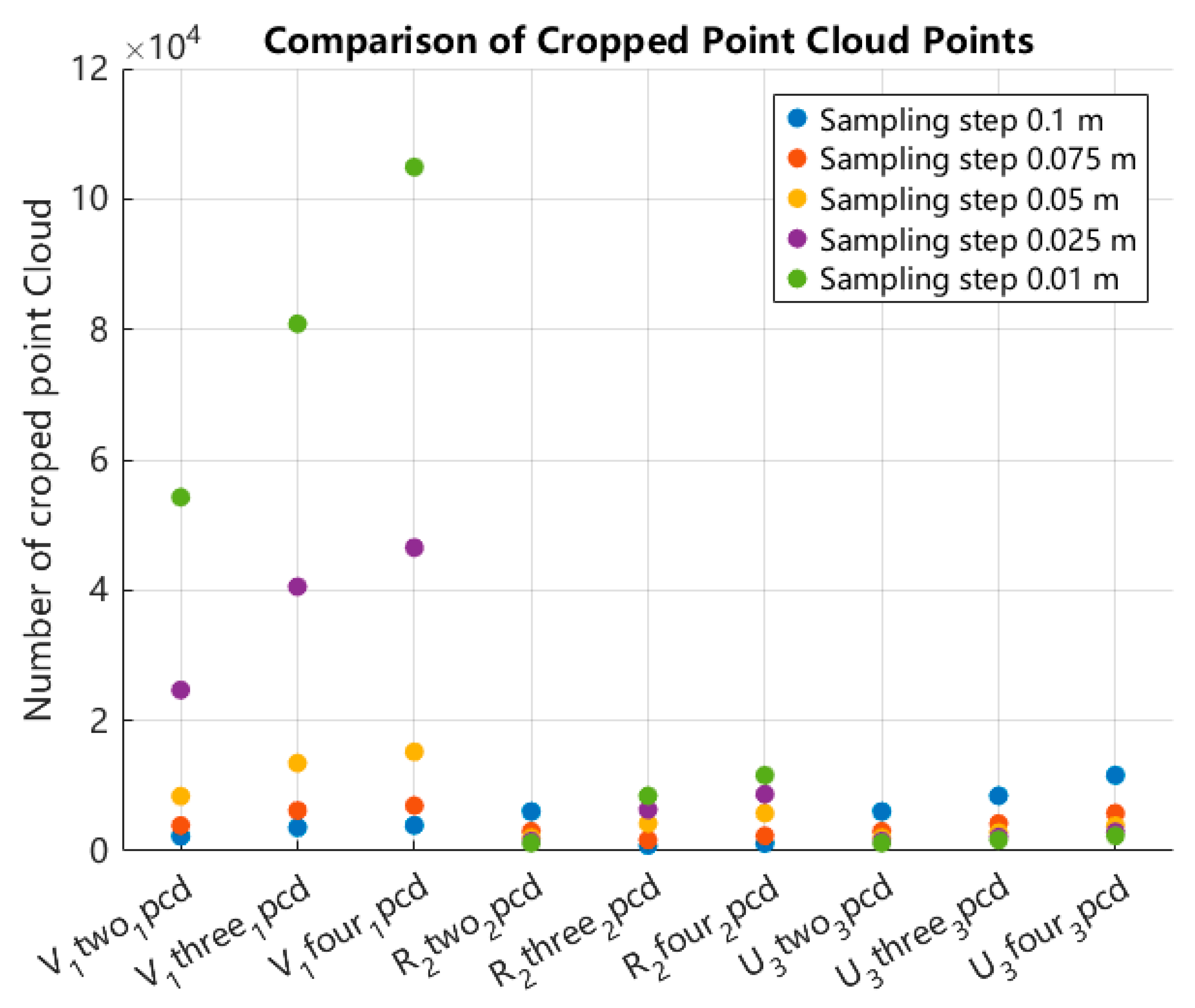
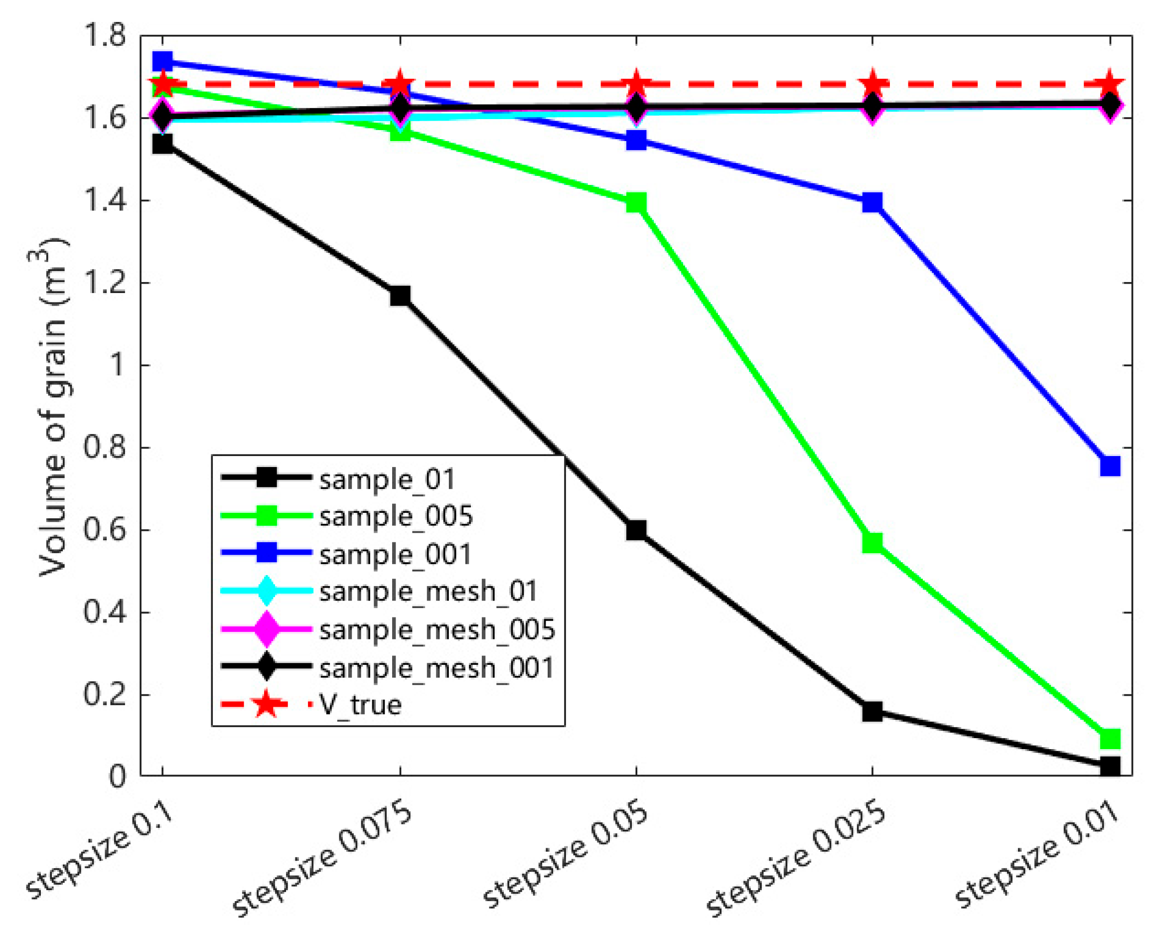
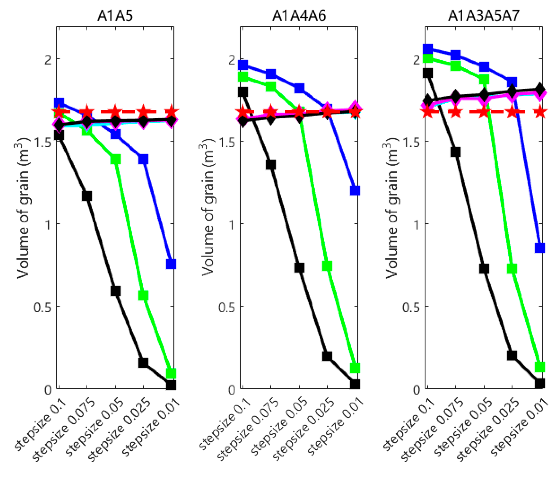
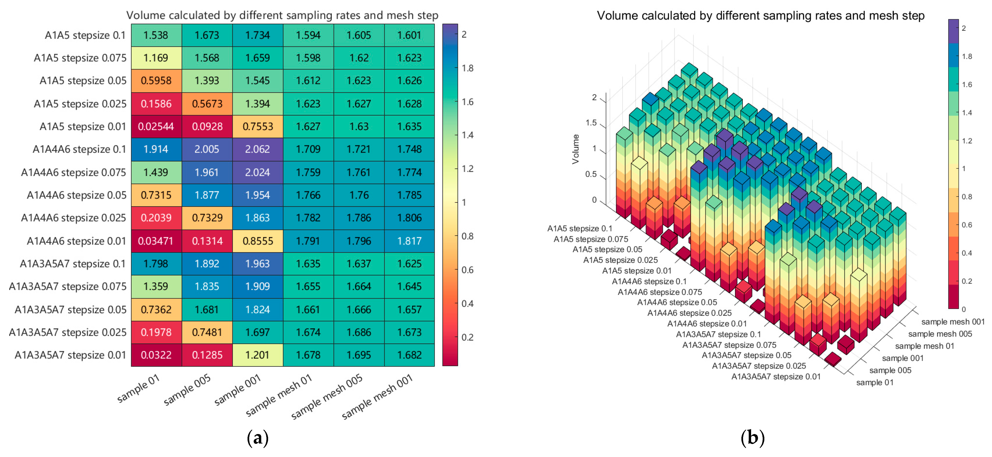
  • Through comparisons of grain pile point clouds obtained by combining 2, 3, and 4 different camera viewpoints, each sampled at step (in meters) lengths of 0.1, 0.075, 0.05, 0.025, and 0.01, and calculating the volume using the BICM method, a maximum error of 6.29%, a minimum error of 1.13%, and an overall average error of 3.39% were achieved. These results demonstrate that the BICM method is an efficient and stable approach for grain pile volume calculation. Therefore, considering measurement efficiency and the minimization of equipment and computational resource usage, it is feasible to achieve a volume calculation error within 5% by employing two opposing viewpoint measurements combined with the BICM method for processing.
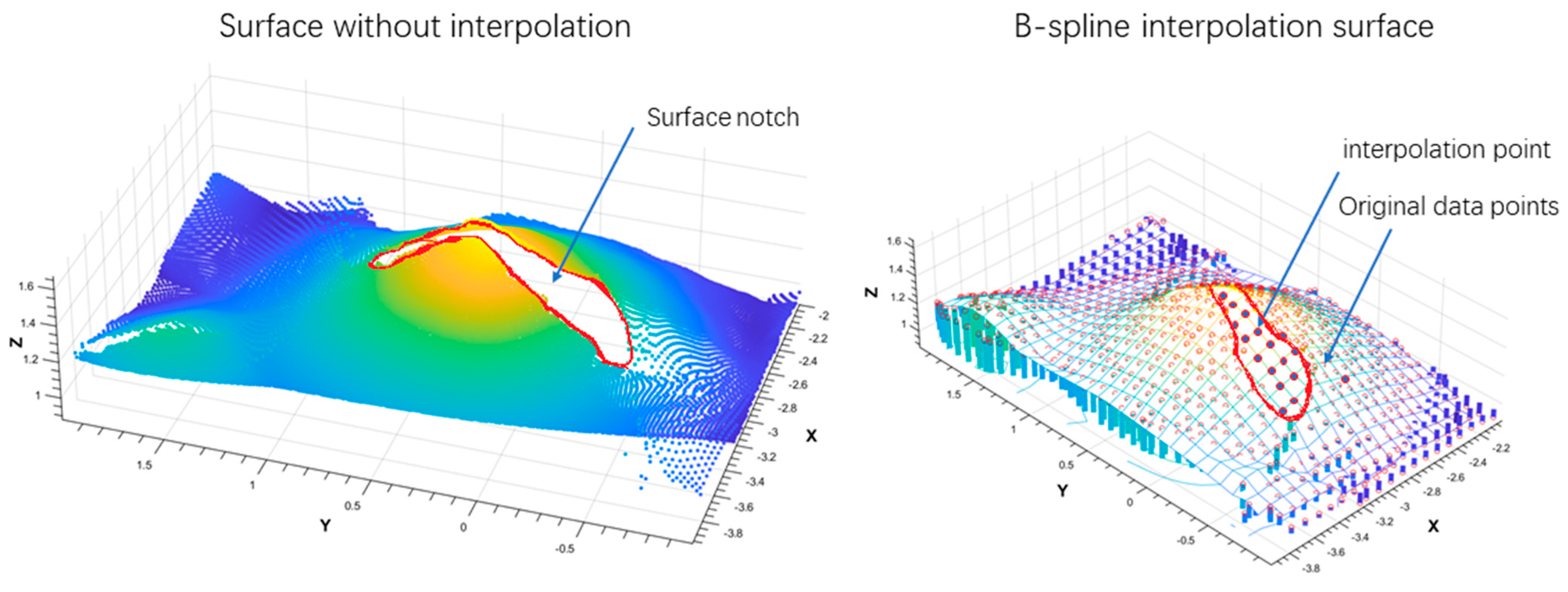
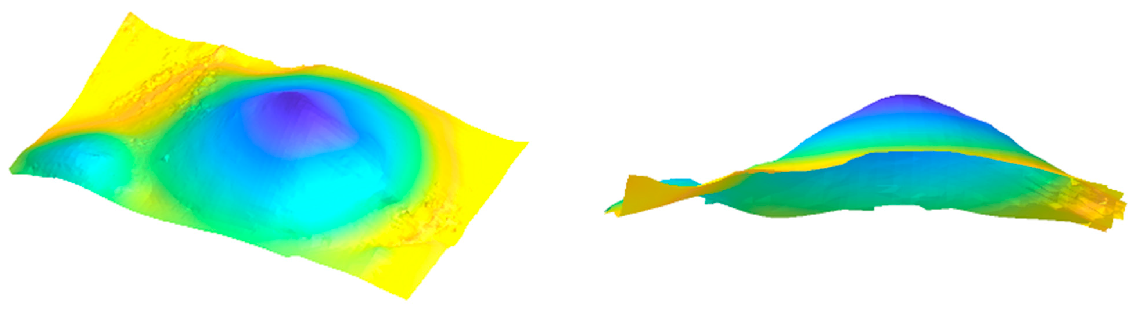
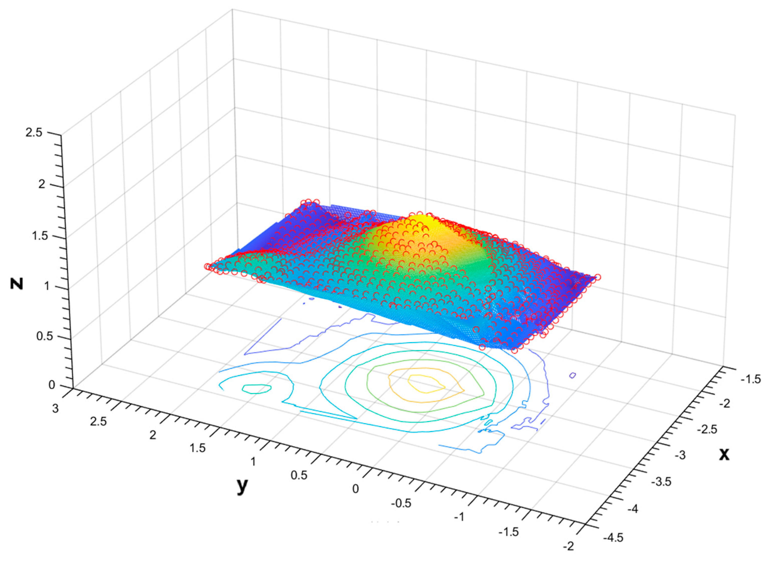
  • The proposed BICM method effectively addresses the issue of significant surface gaps on grain piles by applying B-spline interpolation fitting. It reconstructs smooth and continuous 3D surfaces, successfully overcoming the discontinuities and surface defects caused by the integration of point clouds from multiple camera viewpoints. With its efficient and reliable surface completion performance, the BICM method exhibits strong potential for practical applications in engineering scenarios.
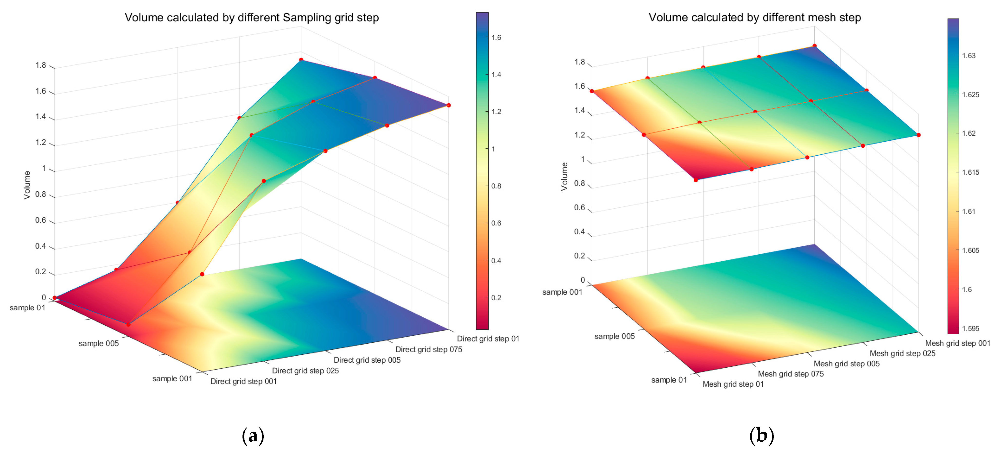
  • By comparing the effects of different sampling step lengths and grid interpolation step lengths on the surface fitting and volume calculation of the grain pile, the relationship between grid interpolation step length and volume calculation accuracy was identified. Specifically, the sampling step length should be matched to the grid interpolation step length, with the optimal configuration determined to be 0.01 m for both.
  • The BICM method enables real-time reconstruction of the 3D model of grain surfaces and grain piles in grain silos, providing essential data for the intelligent management of grain storage, as well as generating 3D maps to support motion planning for robots operating within the silos.

Author Contributions

Conceptualization, L.Y. and W.W.; methodology, L.Y., Z.Y. and F.H.; validation, Z.Y., F.H. and C.R.; formal analysis, L.Y. and W.W.; data curation, C.R., Z.Y. and F.H.; investigation, L.Y. and F.H.; writing—original draft preparation, L.Y., F.H. and Z.Y.; writing—review and editing, C.R., F.H. and L.Y.; supervision, W.W. All authors have read and agreed to the published version of the manuscript.

Funding

This research was supported by the First-Class Discipline Construction Project of Hechi University, Guangxi Industry College of Modern Sericulture and Silk, Guangxi Colleges and Universities Key Laboratory of AI and Information Processing (Hechi University), Education Department of Guangxi Zhuang Autonomous Region, and Proof of Concept of Scientific and Technological Achievements of Jilin University (No. 2024GN023). The authors are highly thankful to the Guangxi Science and Technology Program (No. AA24010001), the Research Project for Young and Middle-Aged Teachers in Guangxi Universities (No. 2024KY0624), the Hechi University research program (No. 2023XJPT010), and the 2024 “Light of Bagui” Study Visit and Training Program (No. [2025] 35) for their financial support.

Data Availability Statement

The original contributions presented in this study are included in the article. Further inquiries can be directed to the corresponding author. The data used to support the findings of this study are available from the corresponding author upon request.

Conflicts of Interest

The authors declare that there are no conflicts of interest.

Appendix A

In three-dimensional space, a rigid body transformation matrix is typically expressed as a 4 × 4 homogeneous transformation matrix, which simultaneously encodes both rotation and translation components. This matrix can be written in the following form:
T = R t 0 T 1 = r 11 r 12 r 13 t x r 21 r 22 r 23 t y r 31 r 32 r 33 t z 0 0 0 1
R 3 × 3 is the rotation matrix, which represents sequential rotations about the z-axis, y-axis, and x-axis, respectively. The translation vector t = [ t x , t y , t z ] T denotes the displacement along each axis. This transformation preserves the rigid structure of an object, maintaining distances and angles during spatial transformations. Based on the spatial configuration of multiple RGB-D cameras in the experimental measurement setup, the transformation matrix was calibrated by integrating the six-axis pose sensors embedded in the cameras and the continuity features of the point cloud. This calibration aimed to minimize the impact of positioning errors as much as possible. The calibrated transformation matrix is given as follows:
Combining the point clouds in the A1A5 direction, the rotate matrix is as follows: rotate= ([0, 186, −5]); the translation matrix is as follows: translate = ([0.2, 0, −5.2]); and the total transformation matrix is as follows:
T 1 = 0.9907 0.0872 0.1041 0.2000 0.0867 0.9962 0.0091 0 0.1045 0 0.9945 5.2000 0 0 0 1.0000
Combining the point clouds in the A1A4A6 direction, the A4 rotate matrix is as follows: rotate1 = ([0, 121.7, −6]); the A4 translation matrix is as follows: translate1 = ([2.89, 0.15, −5.13]); and the A4 total transformation matrix is as follows:
T 2 = 0.5226 0.1045 0.8462 2.8900 0.0549 0.9945 0.0889 0.1500 0.8508 0 0.5255 5.1300 0 0 0 1.0000
The A6 rotate matrix is as follows: rotate2= ([0, −121.7, −5]); the A6 translation matrix is as follows: translate2 = ([−2.35, 0.18, −5.42]; and the A6 total transformation matrix is as follows:
T 3 = 0.5226 0.1045 0.8462 2.3500 0.0549 0.9945 0.0889 0.1800 0.8508 0 0.5255 5.4200 0 0 0 1.0000
Combining the point clouds in the A1A3A5A7 direction, the A3 rotate matrix is as follows: rotate1= ([−4, 90, 6]); the A3 translation matrix is as follows: translate1 = ([2.8, 0, −2.6]); and the A3 total transformation matrix is as follows:
T 4 = 0 0.1736 0.9848 2.8000 0 0.9848 0.1736 0 1.0000 0 0 2.6000 0 0 0 1.0000
The A5 rotate matrix is as follows: rotate2 = ([0, 185, −5]); the A5 translation matrix is as follows: translate2 = ([0.2, 0, −5.3]); and the A5 total transformation matrix is as follows:
T 5 = 0.9924 0.0872 0.0868 0.2000 0.0868 0.9962 0.0076 0 0.0872 0 0.9962 5.3000 0 0 0 1.0000
The A7 rotate matrix is as follows: rotate3 = ([4, −90, 0]); the A7 translation matrix is as follows: translate3 = ([−2.46, 0.13, −2.85]); and the A7 total transformation matrix is as follows:
T 6 = 0 0.0698 0.9976 2.4600 0 0.9976 0.0698 0.1300 1.0000 0 0 2.8500 0 0 0 1.0000

References

  1. Jianyao, Y.; Zhang, Q.; Ge, L.; Chen, J. Technical Methods of National Security Supervision: Grain Storage Security as an Example. J. Saf. Sci. Resil. 2023, 4, 61–74. [Google Scholar] [CrossRef]
  2. Duysak, H.; Yigit, E. Machine Learning Based Quantity Measurement Method for Grain Silos. Measurement 2020, 152, 107279. [Google Scholar] [CrossRef]
  3. Yariv, L.; Kasten, Y.; Moran, D.; Galun, M.; Atzmon, M.; Basri, R.; Lipman, Y. Multiview Neural Surface Reconstruction by Disentangling Geometry and Appearance. Adv. Neural Inf. Process. Syst. 2020, 33, 2492–2502. [Google Scholar]
  4. Pan, Z.; Hou, J.; Yu, L. Optimization Algorithm for High Precision RGB-D Dense Point Cloud 3D Reconstruction in Indoor Unbounded Extension Area. Meas. Sci. Technol. 2022, 33, 055402. [Google Scholar] [CrossRef]
  5. Lutz, É.; Coradi, P.C. Applications of New Technologies for Monitoring and Predicting Grains Quality Stored: Sensors, Internet of Things, and Artificial Intelligence. Measurement 2022, 188, 110609. [Google Scholar] [CrossRef]
  6. Xu, Y.; Nan, L.; Zhou, L.; Wang, J.; Wang, C.C.L. HRBF-Fusion: Accurate 3D Reconstruction from RGB-D Data Using On-the-Fly Implicits. ACM Trans. Graph. 2022, 41, 1–19. [Google Scholar] [CrossRef]
  7. Kurtser, P.; Lowry, S. RGB-D Datasets for Robotic Perception in Site-Specific Agricultural Operations—A Survey. Comput. Electron. Agric. 2023, 212, 108035. [Google Scholar] [CrossRef]
  8. Liu, X.; Li, J.; Lu, G. Improving RGB-D-Based 3D Reconstruction by Combining Voxels and Points. Vis. Comput. 2023, 39, 5309–5325. [Google Scholar] [CrossRef]
  9. Vila, O.; Boada, I.; Coll, N.; Fort, M.; Farres, E. Automatic Silo Axis Detection from RGB-D Sensor Data for Content Monitoring. ISPRS J. Photogramm. Remote Sens. 2023, 203, 345–357. [Google Scholar] [CrossRef]
  10. Huang, T. Fast Neural Distance Field-Based Three-Dimensional Reconstruction Method for Geometrical Parameter Extraction of Walnut Shell from Multiview Images. Comput. Electron. Agric. 2024, 224, 109189. [Google Scholar] [CrossRef]
  11. Yu, S.; Liu, X.; Tan, Q.; Wang, Z.; Zhang, B. Sensors, Systems and Algorithms of 3D Reconstruction for Smart Agriculture and Precision Farming: A Review. Comput. Electron. Agric. 2024, 224, 109229. [Google Scholar] [CrossRef]
  12. Hu, K.; Ying, W.; Pan, Y.; Kang, H.; Chen, C. High-Fidelity 3D Reconstruction of Plants Using Neural Radiance Fields. Comput. Electron. Agric. 2024, 220, 108848. [Google Scholar] [CrossRef]
  13. Hamidpour, P.; Araee, A.; Baniassadi, M. Transfer Learning-Based Techniques for Efficient 3D-Reconstruction of Functionally Graded Materials. Mater. Des. 2024, 248, 113415. [Google Scholar] [CrossRef]
  14. Lyu, X.; Sun, Y.-T.; Huang, Y.-H.; Wu, X.; Yang, Z.; Chen, Y.; Pang, J.; Qi, X. 3DGSR: Implicit Surface Reconstruction with 3D Gaussian Splatting. ACM Trans. Graph. 2024, 43, 1–12. [Google Scholar] [CrossRef]
  15. Kim, J.; Lee, D.; Kwon, S. Volume Estimation Method for Irregular Object Using RGB-D Deep Learning. Electronics 2025, 14, 919. [Google Scholar] [CrossRef]
  16. Miranda, J.C.; Arnó, J.; Gené-Mola, J.; Lordan, J.; Asín, L.; Gregorio, E. Assessing Automatic Data Processing Algorithms for RGB-D Cameras to Predict Fruit Size and Weight in Apples. Comput. Electron. Agric. 2023, 214, 108302. [Google Scholar] [CrossRef]
  17. Yang, M.; Cho, S.-I. High-Resolution 3D Crop Reconstruction and Automatic Analysis of Phenotyping Index Using Machine Learning. Agriculture 2021, 11, 1010. [Google Scholar] [CrossRef]
  18. Yang, T.; Ye, J.; Zhou, S.; Xu, A.; Yin, J. 3D Reconstruction Method for Tree Seedlings Based on Point Cloud Self-Registration. Comput. Electron. Agric. 2022, 200, 107210. [Google Scholar] [CrossRef]
  19. Wu, Z.; Li, H.; Lu, C.; He, J.; Wang, Q.; Liu, D.; Cui, D.; Li, R.; Wang, Q.; He, D. Development and Evaluations of an Approach with Full Utilization of Point Cloud for Measuring the Angle of Repose. Comput. Electron. Agric. 2023, 209, 107799. [Google Scholar] [CrossRef]
  20. Xie, P.; Du, R.; Ma, Z.; Cen, H. Generating 3D Multispectral Point Clouds of Plants with Fusion of Snapshot Spectral and RGB-D Images. Plant Phenomics 2023, 5, 0040. [Google Scholar] [CrossRef]
  21. Yang, D.; Yang, H.; Liu, D.; Wang, X. Research on Automatic 3D Reconstruction of Plant Phenotype Based on Multi-View Images. Comput. Electron. Agric. 2024, 220, 108866. [Google Scholar] [CrossRef]
  22. Li, X.; Liu, B.; Shi, Y.; Xiong, M.; Ren, D.; Wu, L.; Zou, X. Efficient Three-Dimensional Reconstruction and Skeleton Extraction for Intelligent Pruning of Fruit Trees. Comput. Electron. Agric. 2024, 227, 109554. [Google Scholar] [CrossRef]
  23. Zhu, Y.; Cao, S.; Song, T.; Xu, Z.; Jiang, Q. 3D Reconstruction and Volume Measurement of Irregular Objects Based on RGB-D Camera. Meas. Sci. Technol. 2024, 35, 125010. [Google Scholar] [CrossRef]
  24. Hu, H.; Song, A. Digital Image Correlation Calculation Method for RGB-D Camera Multi-View Matching Using Variable Template. Measurement 2025, 240, 115617. [Google Scholar] [CrossRef]
  25. Wei, P.; Yan, L.; Xie, H.; Qiu, D.; Qiu, C.; Wu, H.; Zhao, Y.; Hu, X.; Huang, M. LiDeNeRF: Neural Radiance Field Reconstruction with Depth Prior Provided by LiDAR Point Cloud. ISPRS J. Photogramm. Remote Sens. 2024, 208, 296–307. [Google Scholar] [CrossRef]
  26. Shi, C.; Tang, F.; Wu, Y.; Ji, H.; Duan, H. Accurate and Complete Neural Implicit Surface Reconstruction in Street Scenes Using Images and LiDAR Point Clouds. ISPRS J. Photogramm. Remote Sens. 2025, 220, 295–306. [Google Scholar] [CrossRef]
  27. Qin, K.; Li, J.; Zlatanova, S.; Wu, H.; Gao, Y.; Li, Y.; Shen, S.; Qu, X.; Yang, Z.; Zhang, Z.; et al. Novel UAV-Based 3D Reconstruction Using Dense LiDAR Point Cloud and Imagery: A Geometry-Aware 3D Gaussian Splatting Approach. Int. J. Appl. Earth Obs. Geoinf. 2025, 140, 104590. [Google Scholar] [CrossRef]
  28. Vulpi, F.; Marani, R.; Petitti, A.; Reina, G.; Milella, A. An RGB-D Multi-View Perspective for Autonomous Agricultural Robots. Comput. Electron. Agric. 2022, 202, 107419. [Google Scholar] [CrossRef]
  29. Qi, H.; Wang, C.; Li, J.; Shi, L. Loop Closure Detection with CNN in RGB-D SLAM for Intelligent Agricultural Equipment. Agriculture 2024, 14, 949. [Google Scholar] [CrossRef]
  30. Vélez, S. Integrated Framework for Multipurpose UAV Path Planning in Hedgerow Systems Considering the Biophysical Environment. Crop Prot. 2025, 187, 106992. [Google Scholar] [CrossRef]
  31. Conti, A.; Poggi, M.; Cambareri, V.; Oswald, M.R.; Mattoccia, S. ToF-Splatting: Dense SLAM Using Sparse Time-of-Flight Depth and Multi-Frame Integration. arXiv 2025, arXiv:2504.16545. [Google Scholar]
  32. Storch, M. Comparative Analysis of UAV-Based LiDAR and Photogrammetric Systems for the Detection of Terrain Anomalies in a Historical Conflict Landscape. Sci. Remote Sens. 2025, 11, 100191. [Google Scholar] [CrossRef]
  33. Zhang, N.; Canini, K.; Silva, S.; Gupta, M. Fast Linear Interpolation. J. Emerg. Technol. Comput. Syst. 2021, 17, 1–15. [Google Scholar] [CrossRef]
  34. Klančar, G.; Zdešar, A.; Krishnan, M. Robot Navigation Based on Potential Field and Gradient Obtained by Bilinear Interpolation and a Grid-Based Search. Sensors 2022, 22, 3295. [Google Scholar] [CrossRef]
  35. Li, D.; Cheng, B.; Xiang, S. Direct Cubic B-Spline Interpolation: A Fuzzy Interpolating Method for Weightless, Robust and Accurate DVC Computation. Opt. Lasers Eng. 2024, 172, 107886. [Google Scholar] [CrossRef]
  36. Essanhaji, A.; Errachid, M. Lagrange Multivariate Polynomial Interpolation: A Random Algorithmic Approach. J. Appl. Math. 2022, 2022, 8227086. [Google Scholar] [CrossRef]
  37. Supajaidee, N.; Chutsagulprom, N.; Moonchai, S. An Adaptive Moving Window Kriging Based on K-Means Clustering for Spatial Interpolation. Algorithms 2024, 17, 57. [Google Scholar] [CrossRef]
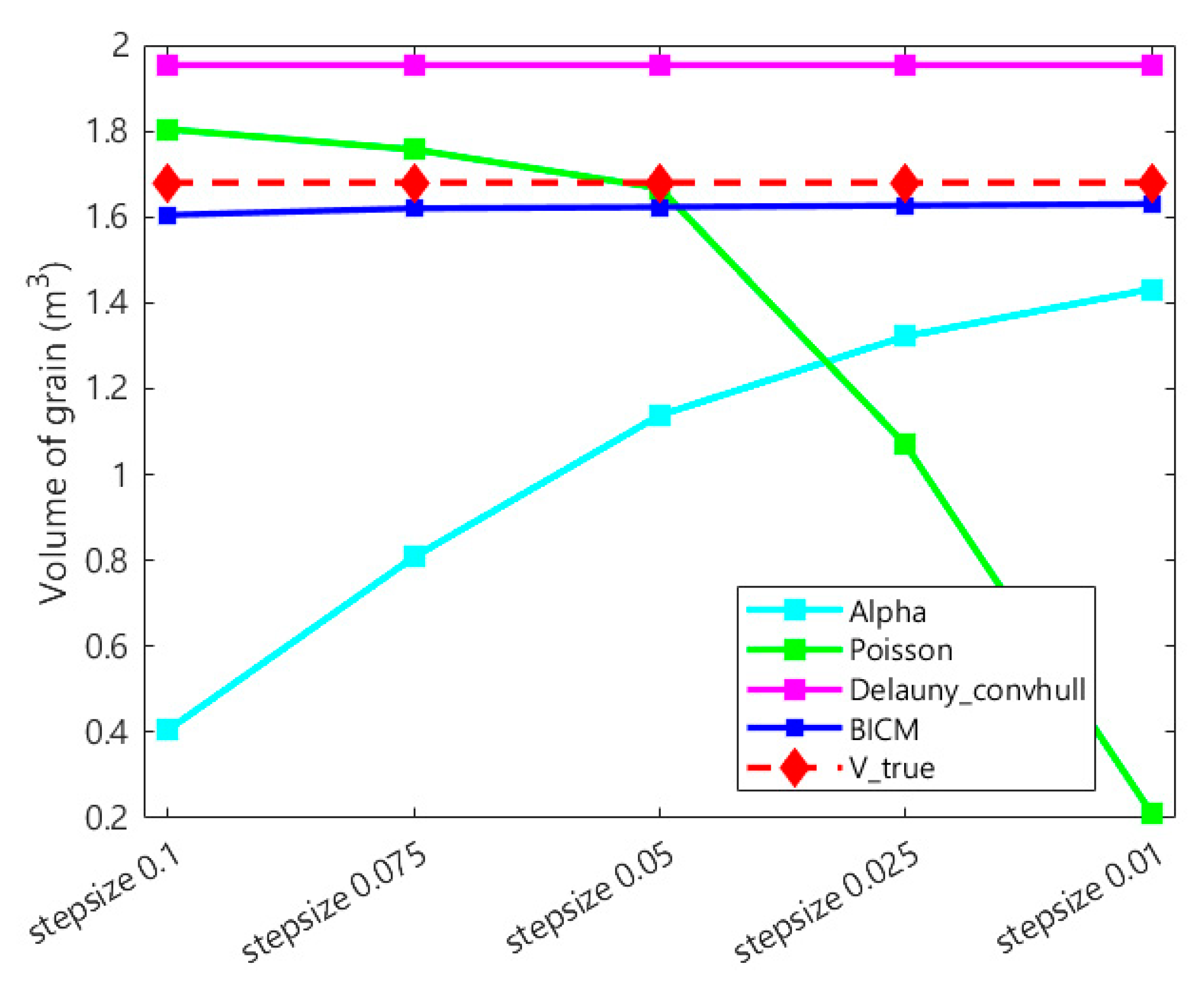
Figure 1. Real scene of the grain pile inside the silo.
Agriculture 15 01208 g001
Figure 2. Point cloud acquired by a single-view RGB-D camera.
Agriculture 15 01208 g002
Figure 3. Combined point cloud from multiple RGB-D camera views.
Agriculture 15 01208 g003
Figure 4. Locally enlarged view of the combined point cloud from two intersecting perspectives.
Agriculture 15 01208 g004
Figure 5. Schematic diagram of the technical workflow.
Agriculture 15 01208 g005
Figure 6. Placement of measurement cameras.
Agriculture 15 01208 g006
Figure 7. Actual measurement scene.
Agriculture 15 01208 g007
Figure 8. Identification of the grain pile and silo robot.
Agriculture 15 01208 g008
Figure 9. Depth map and point cloud obtained from a single RGB-D camera.
Agriculture 15 01208 g009
Figure 10. Point cloud fusion process.
Agriculture 15 01208 g010
Figure 11. Combined point cloud after the first cropping.
Agriculture 15 01208 g011
Figure 12. Point cloud clustering based on distance.
Agriculture 15 01208 g012
Figure 13. Density-based clustering results of multi-view point clouds.
Agriculture 15 01208 g013
Figure 14. Comparison of point cloud down-sampling effects.
Agriculture 15 01208 g014
Figure 15. Coordinate axis transformation of the point cloud.
Agriculture 15 01208 g015
Figure 16. Comparison of different sampling steps in point clouds. (a) A1A5 step size of 0.1 m. (b) A1A5 step size of 0.01 m. (c) A1A3A5A7 step size of 0.1 m. (d) A1A3A5A7 step size of 0.01 m.
Agriculture 15 01208 g016
Figure 17. Position of the cropping box.
Agriculture 15 01208 g017
Figure 18. Combined point cloud after the second cropping. (a) A1A5. (b) A1A4A6. (c) A1A3A5A7.
Agriculture 15 01208 g018
Figure 19. Comparison of point counts before and after point cloud cropping.
Agriculture 15 01208 g019
Figure 20. Fitted surface using B-spline interpolation.
Agriculture 15 01208 g020
Figure 21. Sheet-like surface reconstructed using the Poisson method.
Agriculture 15 01208 g021
Figure 22. Distribution of original data points on the fitted surface.
Agriculture 15 01208 g022
Figure 23. Volume calculation by direct surface enclosure reconstruction: (a) alpha-shape surface fitting method; (b) Delaunay-convex hull surface fitting method.
Agriculture 15 01208 g023
Figure 24. Volume estimation using the cylindrical approximation method.
Agriculture 15 01208 g024
Figure 25. Schematic diagram of equivalent cell height calculation in the grid interpolation method.
Agriculture 15 01208 g025
Figure 26. Comparison of grain pile volumes under different grid steps.
Agriculture 15 01208 g026
Figure 27. Volume of different 3D reconstruction methods.
Agriculture 15 01208 g027
Figure 28. Effects of sampling rate and step size on point cloud volume.
Agriculture 15 01208 g028
Figure 29. Sensitivity comparison of sampling step and grid step to grain pile volume: (a) relationship between sampling step/grid step and volume using the direct rectangular method; (b) relationship between sampling step/BICM grid step and volume.
Agriculture 15 01208 g029
Figure 30. Effects of sampling rate and step size on the volume of different point clouds.
Agriculture 15 01208 g030
Figure 31. Comparison of volume variations under different sampling rates and grid interpolation steps: (a) heat map of volume changes; (b) histogram of volume changes.
Agriculture 15 01208 g031
Table 1. Volume comparison of the grain pile calculated by different 3D reconstruction methods.
Mesh Interpolation StepAlphaPoissonDelaunay_ConvhullBICM
grid_0.10.40571.8041.95381.6046
grid_0.0750.80831.7571.95381.6199
grid_0.051.13831.66711.95381.623
grid_0.0251.32211.06941.95381.6266
grid_0.011.43180.212151.95381.6301
true volume1.680
maximum error73.81%36.35%16.29%4.48%
minimum error14.78%0.77%16.29%2.97%
average error39.21%27.89%16.29%3.52%
Disclaimer/Publisher’s Note: The statements, opinions and data contained in all publications are solely those of the individual author(s) and contributor(s) and not of MDPI and/or the editor(s). MDPI and/or the editor(s) disclaim responsibility for any injury to people or property resulting from any ideas, methods, instructions or products referred to in the content.

