Article

Flow Control of Tractor Multi-Channel Hydraulic Tester Based on AMESim and PSO-Optimized Fuzzy-PID

1
College of Engineering, Nanjing Agricultural University, Nanjing 210031, China
2
Jiangsu Province Agricultural Machinery Test and Identification Station, Nanjing 210017, China
*
Author to whom correspondence should be addressed.
Agriculture 2025, 15(11), 1190; https://doi.org/10.3390/agriculture15111190
Submission received: 16 March 2025 / Revised: 26 May 2025 / Accepted: 28 May 2025 / Published: 30 May 2025
(This article belongs to the Section Agricultural Technology)

Abstract

To improve the dynamic response, linearity, and control accuracy of the YYSCT-250-3 tractor multi-circuit hydraulic output power tester, this study develops a particle swarm optimization (PSO)-tuned fuzzy-proportional–integral–derivative (Fuzzy-PID) control strategy. By modulating the actuator-driven ball valve’s rotation angle (0–90°) in the proportional flow valve, the controller uses both the flow rate error and its rate of change between the setpoint and the flow meter feedback as fuzzy inputs to adjust the PID outputs. A detailed mathematical model of the electro-hydraulic proportional flow system is established, incorporating hydraulic resistance torque on the ball valve spool and friction coefficients to enhance accuracy. Through MATLAB/Simulink (R2022a) simulations, the PSO algorithm optimizes the fuzzy membership functions and PID gains, yielding faster response, reduced overshoot, and minimal steady-state error. The optimized controller achieved relative steady-state flow errors within ±1.0% and absolute flow control errors within ±0.5 L/min, significantly outperforming the traditional PID controller. These results demonstrate that the PSO-optimized Fuzzy-PID approach effectively addresses the flow control challenges of the YYSCT-250-3, enhancing both testing efficiency and precision. This work provides a robust theoretical framework and practical reference for rapid, high-precision flow control in multi-channel hydraulic power testing.

1. Introduction

The YYSCT-250-3 tractor multi-circuit hydraulic output power tester (Nanjing, Jiangsu, China) is vital equipment for inspecting agricultural machinery and advancing agricultural modernization. Precise flow control is a core aspect of precision agriculture, directly affecting system reliability and stability. However, existing testers still rely on conventional PID strategies for flow control, which suffer from accuracy limitations due to frictional losses between the proportional flow valve and its seat—ultimately compromising output power performance and stability [1,2].
Electro-hydraulic proportional flow valves serve as the core components of hydraulic systems, and their control accuracy directly influences overall system performance. In recent years, driven by the growing demand for smart agriculture and precision agricultural machinery, researchers both domestically and internationally have made significant advances in electro-hydraulic proportional flow valve control: Wang et al. [3] introduced a segmented PID control strategy utilizing working flow rate feedback. Through extensive experimental validation, they demonstrated that this approach delivers superior flow control accuracy and fertilization precision compared to constant-speed systems, albeit at the cost of increased overshoot. Soren Ketelsen et al. [4] developed a pump-controlled differential cylinder drive system to enhance response speed; however, it remains inadequate in terms of precise flow control, model fidelity, and on-vehicle validation. Sun [5] proposed a sliding-mode control method based on the adaptive reaching law to address the nonlinearity and parameter uncertainties in the electro-hydraulic position-servo system, thereby enhancing the system’s control precision and robustness. Li et al. [6] designed a hydraulic proportional flow valve with pressure-compensation functionality, but the improvement in flow response time was limited. These studies have mostly focused on the design and simulation stages, with few actual experimental applications, and have not effectively addressed issues such as nonlinearity and time delay. However, existing studies mainly suffer from two key limitations: (1) traditional optimization algorithms struggle to balance multi-objective conflicts (e.g., references [3,4,5] fail to address the trade-offs among response speed, overshoot, and steady-state accuracy); (2) the dynamic coupling between the rotational resistance torque and the friction coefficient of the proportional valve is not considered (e.g., reference [6]). These limitations, to some extent, restrict the effectiveness of existing methods in full-condition adaptive control and complex nonlinear compensation scenarios.
For the limitations of traditional PID algorithms, PID improvement schemes based on fuzzy control theory have received widespread attention for their superior stability and suitability for nonlinear systems [7,8,9,10,11,12]. For instance, Luo et al. [13] employed feedforward Fuzzy-PID to address nonlinearities in microbial fuel cell systems, ensuring rapid voltage stabilization. Ghasemi et al. [14] proposed a Fuzzy-PID control method based on nonlinear dynamic analysis, which enhances the response speed and steady-state accuracy of traditional control approaches under nonlinear and time-varying conditions. Peng et al. [15] addressed the asymmetric characteristics of an electro-hydraulic servo-valve cylinder system by employing a dual-fuzzy algorithm to compensate for its control deficiencies. In multi-channel coupled hydraulic systems such as the YYSCT-250-3, the design of control strategies faces unique challenges: (1) strong nonlinear disturbances caused by spool vibrations resulting from hydraulic shocks and pressure fluctuations induced by fluid pulsations; (2) time-varying parameters arising from sudden field load variations (40–200 L/min) and oil temperature changes (−20 °C to 60 °C); and (3) the inherent trade-off between response speed and overshoot suppression.
Although Niu Bin [16] enhanced valve control accuracy by integrating PID and fuzzy logic, the rule base still depends on empirical knowledge. Hou Yuanxin et al. [17] proposed a neural-network-based PID method with self-adaptive parameters, but it suffers from high computational complexity. Mounce et al. [18] demonstrated the effectiveness of GA–fuzzy control in drainage networks; however, it did not address the friction–flow coupling effect unique to hydraulic systems [19,20,21,22,23,24,25].
Therefore, the research objectives of this study are as follows:
(1)
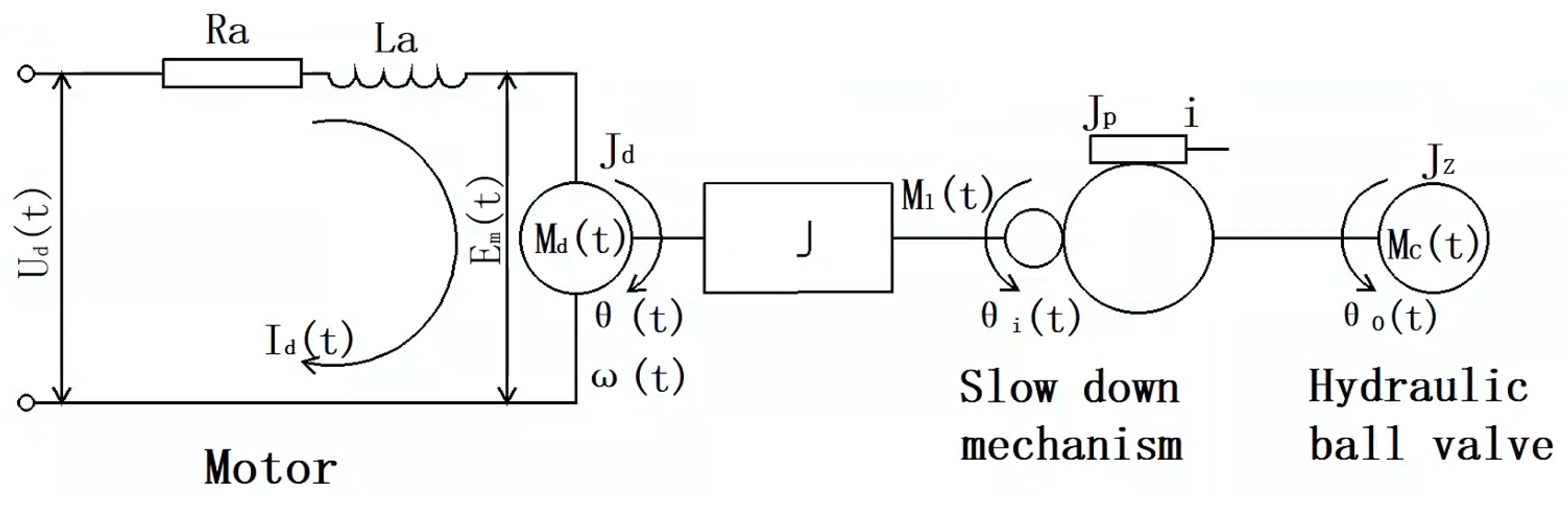
Modeling level: A dynamic torque equation for the ball valve considering the friction coefficient is established, and a modified transfer function model integrating hydraulic fluid force and damping effects is derived to improve the modeling accuracy and dynamic response analysis capability of the hydraulic control system.
(2)
Simulation level: On the co-simulation platform of AMESim2020.1 and MATLAB/Simulink, a PSO-based multi-objective fitness function is constructed to perform Pareto-optimal searching for fuzzy quantization factors and PID parameters, thereby enhancing the precision and efficiency of control parameter optimization.
(3)
Engineering application level: A hardware-in-the-loop (HIL) testing platform based on the OLE for process control (OPC) protocol is developed to address parameter transfer issues between the simulation environment and real vehicle working conditions, thereby improving the adaptability and reliability of the control strategy in engineering applications.
In summary, this study addresses the nonlinear coupling and control accuracy issues of the YYSCT-250-3 system by integrating model correction, algorithm optimization, and engineering platform development, thereby enhancing the intelligence and control performance of agricultural hydraulic equipment [26,27,28]. The structure of this paper is organized as follows: Section 2 introduces the system structure and operating principles; Section 3 establishes the valve transfer function model; Section 4 designs the flow controller; Section 5 presents simulations and experiments; and Section 6 provides the conclusions.

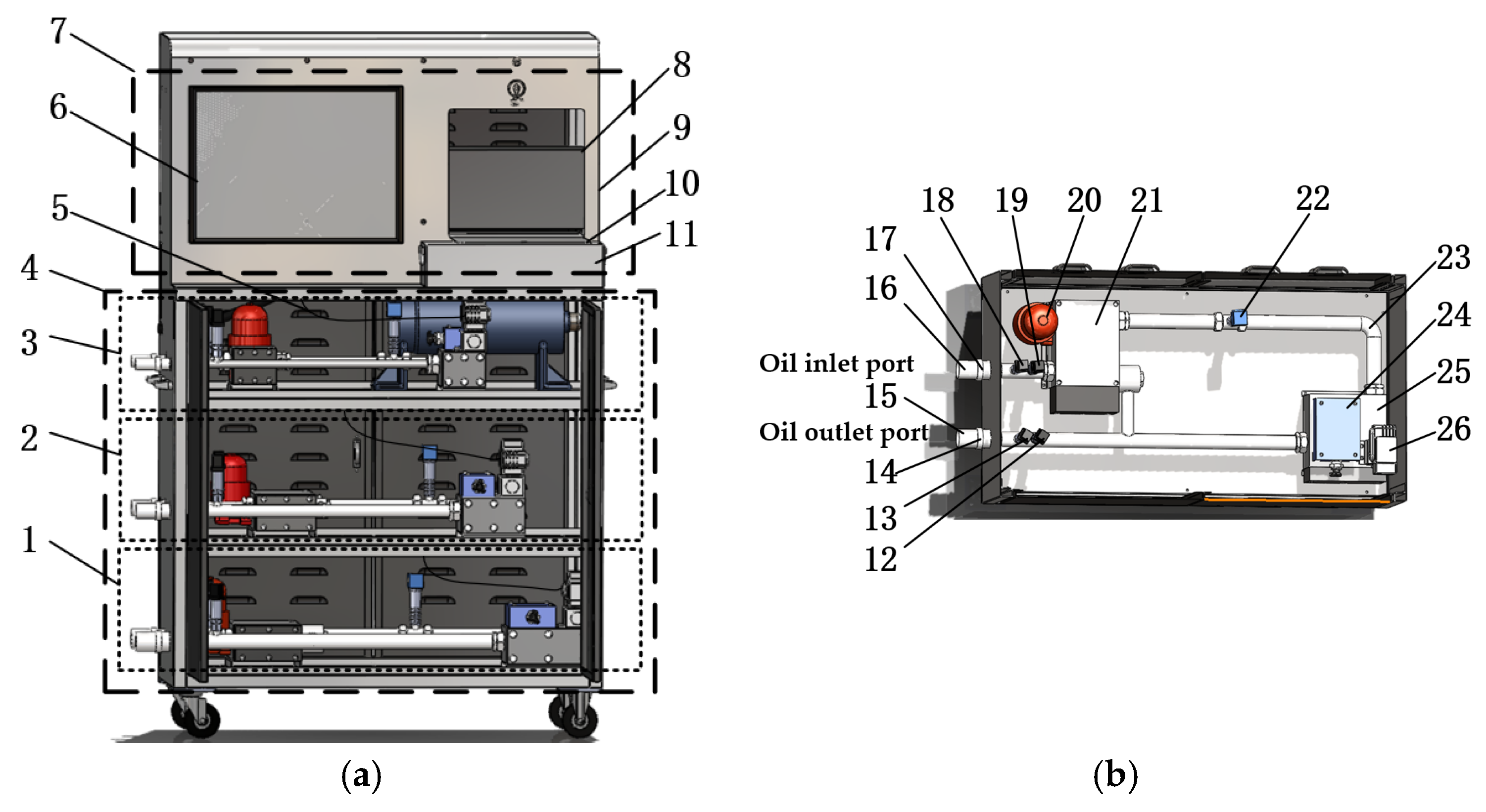
2. Structure and Working Principle of YYSCT-250-3

2.1. Structure of YYSCT-250-3

The overall structure of the YYSCT-250-3 studied here consists of a control–display unit, a measurement unit, and an enclosure. The control–display unit is mounted on the upper part of the enclosure, while the measurement unit is installed on the lower part; the two are linked by communication cables. The complete tester assembly is shown in Figure 1.
The control–display unit comprises an industrial all-in-one touchscreen, communication cables, a printer, and a PLC controller. The measurement unit consists of three tractor hydraulic output-power measurement modules for high, medium, and low flow rates. Each measurement module includes a quick-release coupling, inlet hose, high-pressure hose, pressure sensor, temperature sensor, filter, flow meter, proportional flow valve, relief valve, check valve, and return hose. Hydraulic oil flows through the inlet hose, the components of the measurement module, and the return hose to form the hydraulic output-power test circuit. The proportional flow valve system refers to the electro-hydraulic proportional flow valve shown as item 26 in Figure 1b; it consists of a hydraulic ball valve, an electric actuator, a Fuzzy-PID controller, and associated hardware.
The YYSCT-250-3 measures output power via the pressure differential between its inlet and outlet ports, as depicted in Figure 1b. The key component controlling hydraulic oil flow is the electro-hydraulic proportional flow ball valve (26), which is installed in Measurement Unit 4 in Figure 1a. Measurement Unit 4 comprises three sub-systems—high-, medium-, and low-flow hydraulic test systems—each covering a different flow range; flow is regulated by adjusting the valve’s opening. The main performance parameters of the YYSCT-250-3 are listed in Table 1.

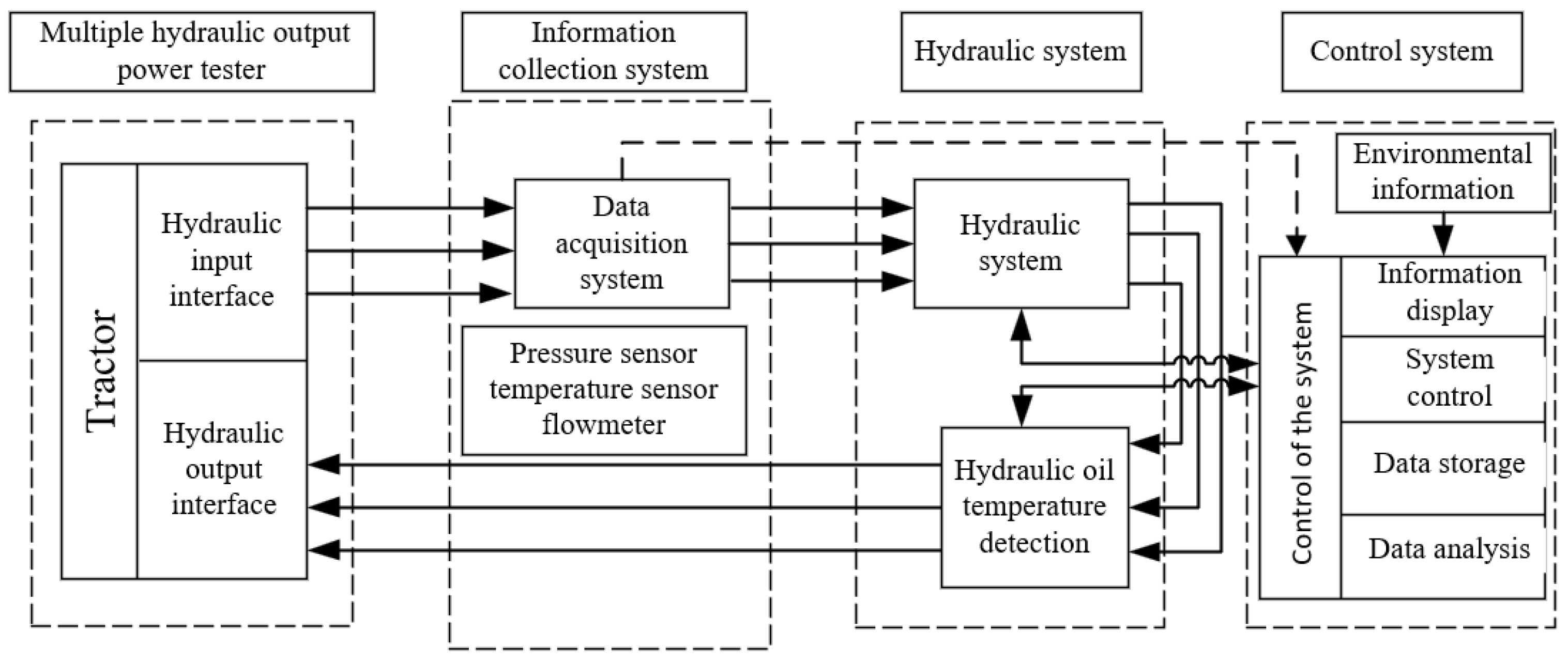
2.2. Composition of Hydraulic Output Power Tester Parameter Detection

The performance parameter detection equipment for tractor multi-circuit hydraulic output devices mainly consists of three parts: an information acquisition system, a hydraulic system, and a control system, as shown in Figure 2.
Information collection system: Primarily composed of hydraulic oil temperature sensors, pressure sensors, flow sensors, and data acquisition cards, it collects key information and processes data in real time, transmitting them to the control system. The collection of performance parameters involves theoretical analysis, sensor selection, and information acquisition and conditioning technologies to meet the design and testing requirements of tractor hydraulic systems.
Hydraulic System: Mainly includes relief valves, electro-hydraulic proportional control valves, oil tanks, and temperature control systems.
Control System: The test control interface features key parameter displays, key parameter curves, and control areas, facilitating real-time operation and data display during testing.

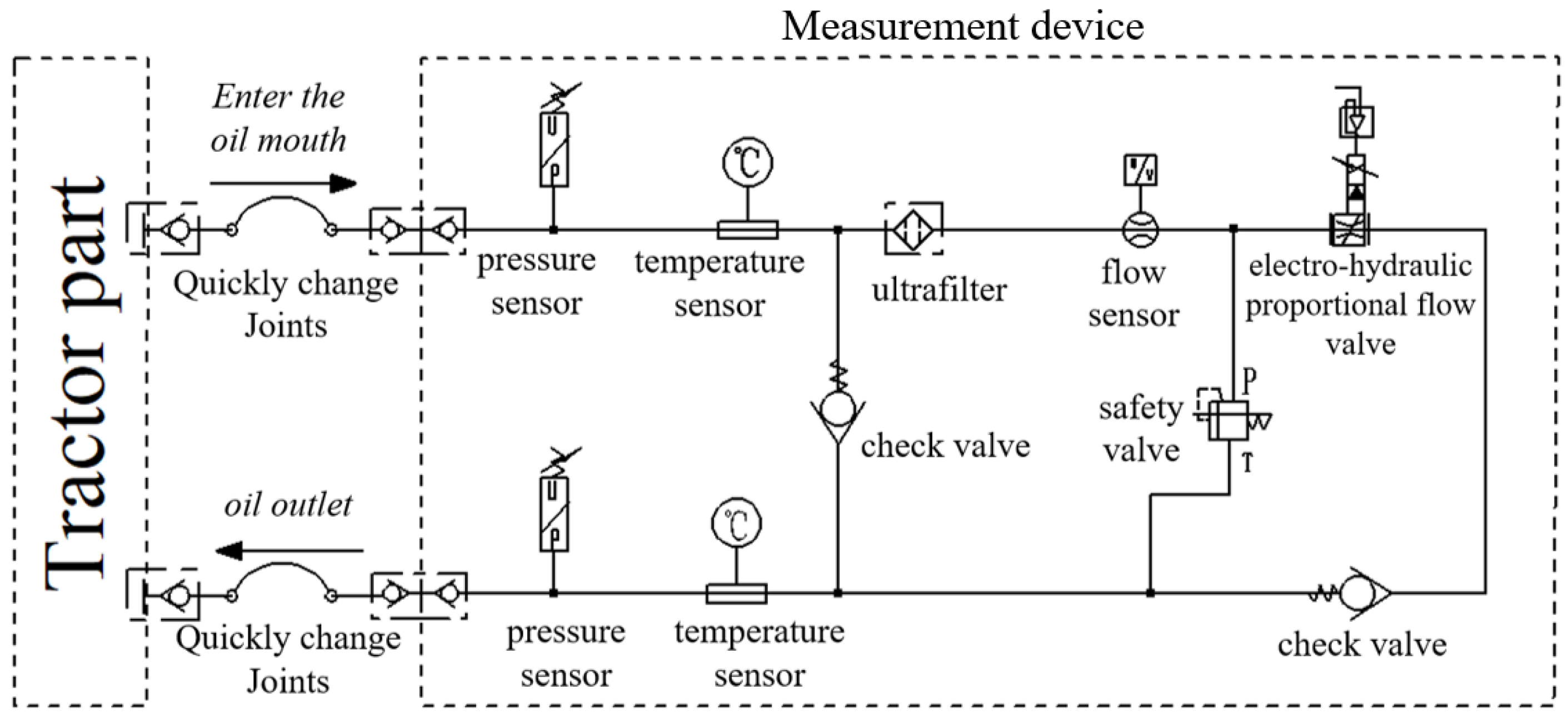
2.3. Working Principle of YYSCT-250-3

By adjusting the opening of the proportional flow valve on the hydraulic output tester to regulate circuit flow, and calculating hydraulic output power from the relationship between power, flow, and pressure, the YYSCT-250-3 achieves improved testing accuracy and efficiency across different horsepower and flow ranges. Its hydraulic testing principle is illustrated in Figure 3.
The maximum effective hydraulic power P through a pair of hydraulic connectors is calculated using Equation (1):
  P = ( P 1 P 2   ) Q 60   η
where P is effective hydraulic power through a pair in kW (kW); P1 is pressure at the hydraulic connector near the tractor output (MPa); P2 is the pressure at the hydraulic connector near the tractor input (MPa); Q is measured flow rate (L/min); η is the hydraulic output power correction coefficient, obtained from pipeline power losses.

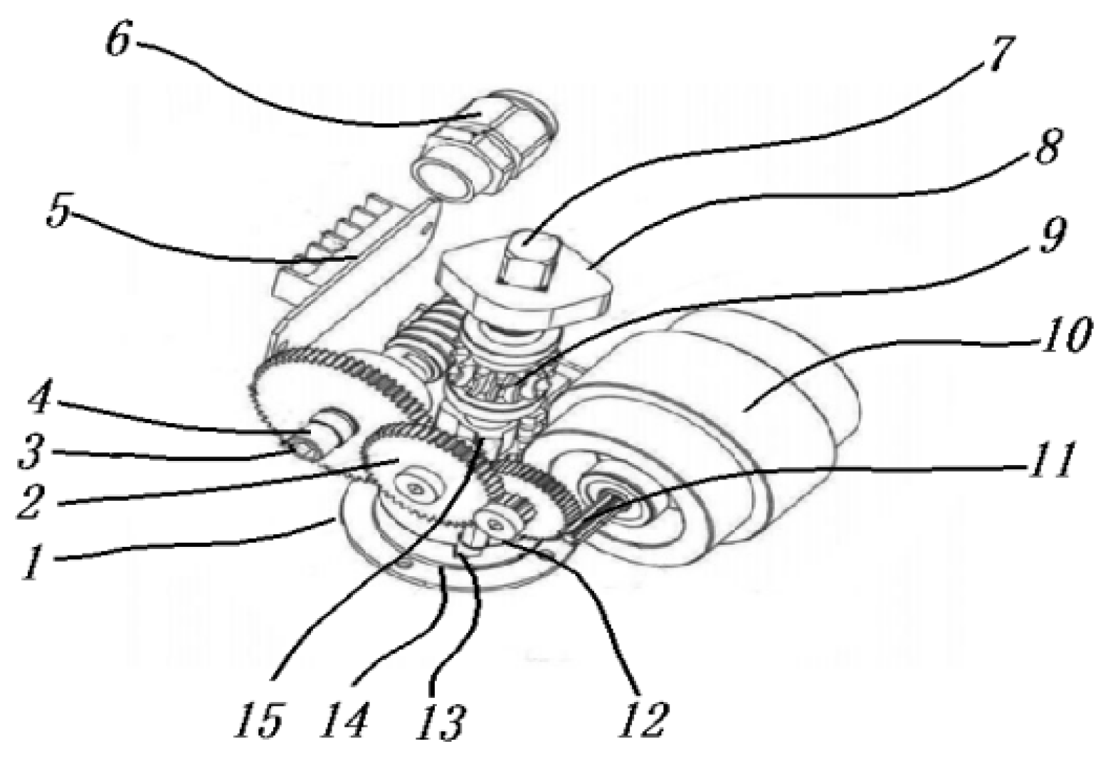
3. Working Principle and Transfer Function Model of Electro-Hydraulic Proportional Flow Valve

3.1. Working Principle of Electro-Hydraulic Proportional Flow Valve

The torque output by the electric actuator is transmitted directly to the hydraulic ball valve spool, and its resulting angular displacement corresponds to the rotation angle of the valve spool.
Relative   opening   of   valve   cell = θ 90 ° × 100 %
where θ is valve core angle (°).
By deriving the mathematical model of the electric actuator, the relationship between its output angular displacement and the applied voltage was established, thereby enabling control of the flow valve opening via voltage adjustment. The motor, driven by armature input voltage, produces torque on its shaft; this torque is first transmitted through a gearbox reduction mechanism to the worm, then through a worm-and-wheel reduction stage to the ball valve stem, causing the valve spool to rotate and alter the flow area, thus regulating flow. The internal structure of the electric actuator is shown in Figure 4.
The drive motor in the electric actuator is a DC servomotor, which offers high energy efficiency, excellent start–stop performance, a favorable mechanical time constant, and high-precision speed and position control. It is widely used in actuators of digital control systems to achieve precise constant-speed regulation and electronically driven speed profiles.

3.2. Construction of the Transfer Function Model for Electro-Hydraulic Proportional Flow Valve

The electric actuator consists of two main components—the motor and the worm-and-wheel reduction gearbox. Figure 5 shows the mathematical model of the electro-hydraulic proportional flow valve system, and the derived transfer function between the input voltage and the output angular displacement is as follows:
The dynamic balance equation of the DC motor, based on Kirchhoff’s law, yields the voltage balance equation:
U d ( t ) = R a I d ( t ) + L a d I d ( t ) d t + E m ( t )
where U d is the motor armature input voltage (V), R a is the armature winding resistance (Ω), I d is the current (A) flowing through the armature winding, L a is the armature winding inductor (H), and E m is the motor induction counter potential (V).
Based on the law of magnetic field action on current-carrying coils, the torque equation is:
M d ( t ) = K m I d ( t )
where M d is the motor output torque (N·m), and K m is the torque coefficient of electric motor (N·m/A).
By applying Newton’s second law for rotational motion, a torque equation is established. Since relative movement between the valve spool and seat generates frictional force—which can degrade control precision—the angular control of the ball valve must account for the spool’s inertial torque, fluid-induced damping torque, and the motor’s friction coefficient, while neglecting fluid forces and friction between seals and the valve stem. The motor’s friction coefficient is incorporated into the system transfer function and is primarily influenced by the materials chosen for the spool and seat. The relevant parameters are listed in Table 2.
M d ( t ) M l ( t ) J z · d 2 θ d t 2 C · d θ d t F f F m = J m d w ( t ) d t
M l = f w ( t )
where M l ( t ) is the load torque on the input shaft of the reduction mechanism (N·m), J m is the motor’s moment of inertia (kg·m2), ω ( t ) is the motor speed (r/min). Based on the torque balance equation, substituting Equation (6) into Equation (5) yields the differential equation for the rotation angle:
M d ( t ) = ( J m + J z ) θ ¨ ( t ) + ( f + C ) θ ˙ ( t ) + F f + F m
where θ ( t ) is the motor output rotation angle (rad), f is the motor viscosity friction coefficient (N·m·s/rad), M c is the load moment (N·m) of the ball valve, J is the motor shaft moment of inertia (kg·m2), and J z is the inertia of rotation of the ball valve core (kg·m2).
J Z = r 2 · d m
where r is the radius of each point on the valve core, and dm is the infinitesimal mass element. C is the damping coefficient of the mechanical system and hydraulic fluid acting on the valve rotation. According to the structure of this ball valve, this coefficient is taken as 0.55. F f is the fluid force term, and the pressure difference and flow change of hydraulic fluid in the pipeline determine the fluid force. The fluid force is expressed as follows:
F f = Δ P · A = Δ P · θ   ( t ) 90 · A
Δ P is the pressure difference of the inlet and outlet, which changes with the opening of the ball valve. It is calculated by the Bernoulli equation and the pipeline hydrodynamic formulation. A is the effective force area and depends on the opening of the valve.
A = D   2 · β
where β is the geometric opening coefficient, varying with the angle θ . For circular section valves, flow is obtained directly by the sensor; F m is a friction force term; due to the friction between seals or stems, the expression of the friction force is:
F m = μ · N ( θ ) · c o s θ
μ is the friction coefficient, determined by the material and the working environment, and N is the forward force, derived from the pretension force of seals and fluid pressure. When the ball valve rotates to an angle θ, the effective component of the forward force in the vertical direction of the sealing surface becomes N θ · c o s θ .
Substituting Equation (7) into Equation (4) yields the differential equation of the rotation angle:
I d ( t ) = 1 K m ( J m + J z ) θ ¨ ( t ) + ( f + C ) θ ˙ ( t ) + F f + F m
Substituting Equation (12) into Equation (3) yields the differential equation of the rotation angle.
U d ( t ) = R a K m ( J m + J Z ) θ ¨ ( t ) + ( f + C ) θ ˙ ( t ) + F f + F m + L a K m ( J m + J Z ) θ ( t ) + ( f + C ) θ ¨ ( t ) + E m ( t )
E m = K e θ ˙ ( t )
where K e is the anti-potential coefficient of the motor (V/rad).
Integrate Formula (14) into Formula (13) to obtain the differential equation between the motor rotation angle and the voltage:
( L a J m + L a J z ) θ ( t ) + ( R a J m + R a J z + L a f + L a C ) θ ¨ ( t ) + ( R a f + K m K e + R a C ) θ ˙ ( t ) + R a ( Δ P · θ ( t ) 90 · A + μ · N ) = K m U d ( t )
Taking the Laplace transform of the above equation yields the following equilibrium equation:
( L a J m + L a J z ) s 3 θ ( s ) + ( R a J m + R a J z + L a f + L a C ) s 2 θ ( s ) + ( R a f + K m K e + R a C ) s θ ( s ) + R a · Δ P · θ ( s ) 90 A + R a · μ · N = K m U d ( s )
After simplification, the transfer function between the angle and voltage of the armature-controlled DC motor is obtained:
Θ ( s ) U ( s ) = K m ( L a J m + L a J z ) s 3 + ( R a J m + R a J z + L a f + L a C ) s 2 + ( R a f + K m K e + R a C ) s + R a · Δ P · A 90 R a · μ · N s
After the motor shaft delivers torque to the reduction mechanism’s input shaft, it is first slowed by the gear reduction stage, then further decelerated and torque-multiplied by the worm-and-wheel stage, and finally transmitted via the reduction mechanism’s output shaft to the valve stem, driving the valve spool to rotate. The following relationship applies:
i = M c M l = θ i θ o = w i w o
where i is the transmission ratio of the deceleration mechanism, θ i is the input shaft angle (rad) of the deceleration mechanism, θ o is the ball valve core shaft angle (rad), ω i is the input shaft speed of the deceleration mechanism (r/min), and ω o is the output shaft speed of the deceleration mechanism (r/min).
The relation between input and output corners of the deceleration mechanism is:
θ ( s ) θ o ( s ) = i
By combining Equations (17) and (19), the transfer function of the electro-hydraulic proportional flow valve system’s electric actuator is obtained:
G ( s ) = Θ O ( s ) U ( s ) = K m i ( L a J m + L a J z ) s 3 + ( R a J m + R a J z + L a f + L a C ) s 2 + ( R a f + K m K e + R a C ) s + R a · Δ P · A 90
The system friction coefficient has the following relationship:
f = Δ M d ( t ) + M c ( t ) i   η w
In the equation, η represents the transmission efficiency of the drive mechanism.
According to the law of conservation of energy, there are:
1 2 J O w O     2 = 1 2 J i   w i       2 η
The moment of inertia on the output side is converted to the input side as follows:
J i = J O i η
The system moment of inertia has the following relationship:
J   = J m + J p + J z i η
where J m is the moment of inertia of the motor shaft (kg·m2), J p is the moment of inertia of the reducer converted to the motor shaft (kg·m2), J z is the moment of inertia of the load ball valve (kg·m2). The complete transfer function of the electric actuator is obtained combined with the DC servo motor and the reduction mechanism:
G ( s ) = Θ o ( s ) U ( s ) = K m i ( L a J m + L a J z ) s 3 + ( R a J m + R a J z + L a f + L a C ) s 2 + ( R a f + K m K e + R a C ) s + R a · Δ P · A 90 R a · μ · N i s
The transfer function establishes the relationship between the valve core’s angular displacement and the motor voltage, enabling control of the electro-hydraulic proportional flow valve’s opening by adjusting the voltage.

3.3. Parameter Selection for Electric Actuator

Based on the torque, rotation angle, and speed requirements of the hydraulic ball valve, NT-5 series (50 N·m) and NT-10 series (100 N·m) electric actuators were selected. The hydraulic tester is equipped with three flow segments (inner diameters of 32 mm, 25 mm, and 10 mm), with maximum flow rates of 250 L/min, 166 L/min, and 100 L/min, respectively. At a flow rate of 100 L/min, the ball valve requires an input torque of 50 N·m; at 166 L/min and 250 L/min, the required input torque is 100 N·m. The valve core has a rotation stroke of 90°, and the main parameters of the electric actuators are listed in Table 2.
By substituting the values from Table 2 into Equation (25), the specific transfer functions for the NT-5 and NT-10 electric actuators used in the electro-hydraulic proportional flow valves are obtained.

4. Design of Electro-Hydraulic Proportional Flow Controller

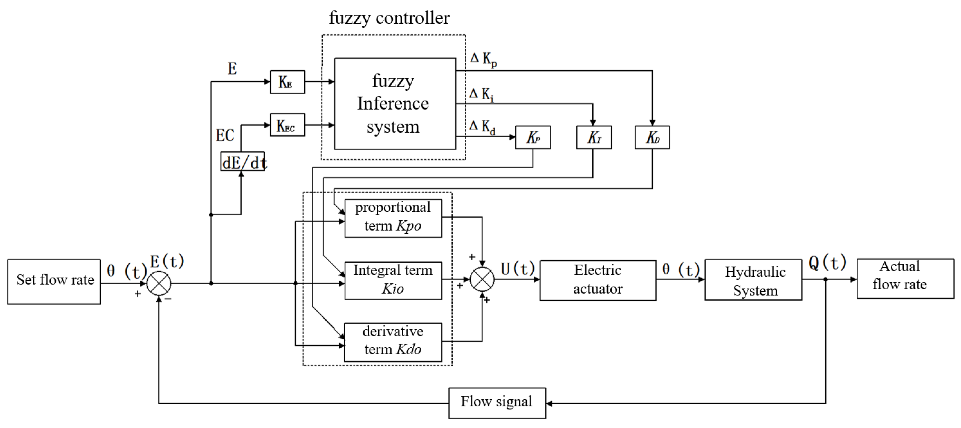
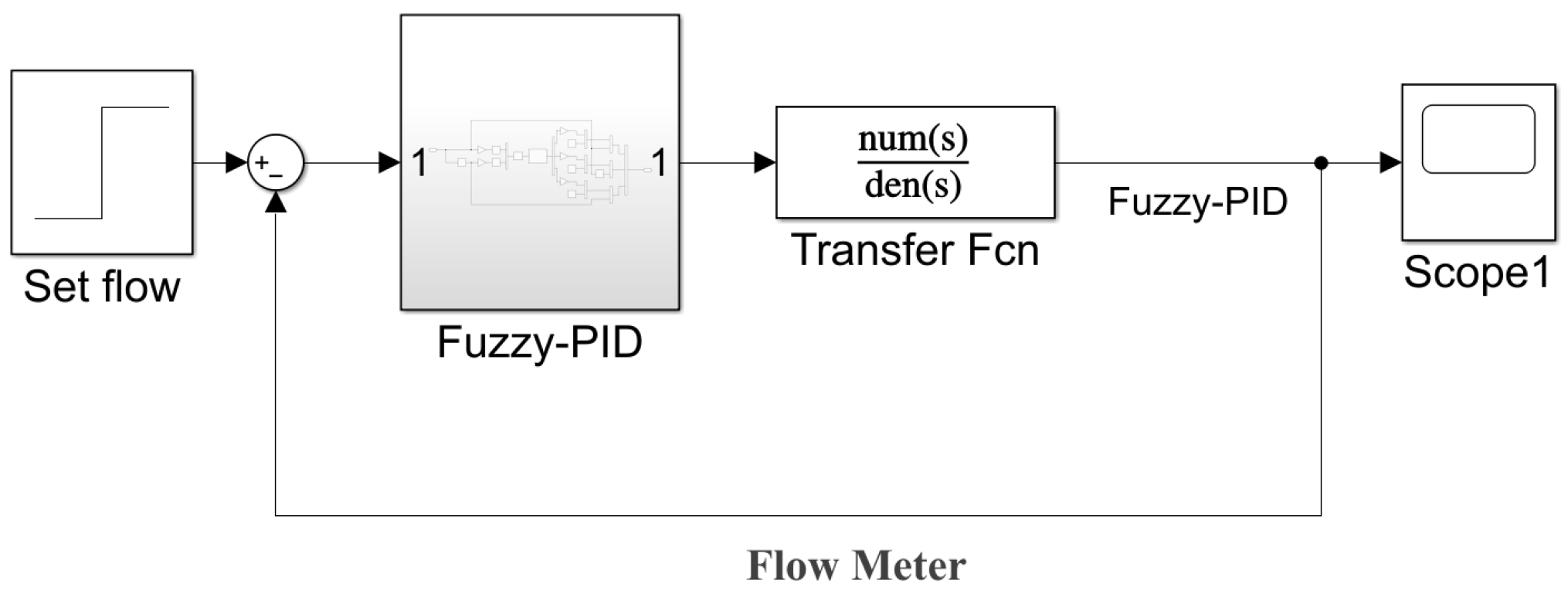
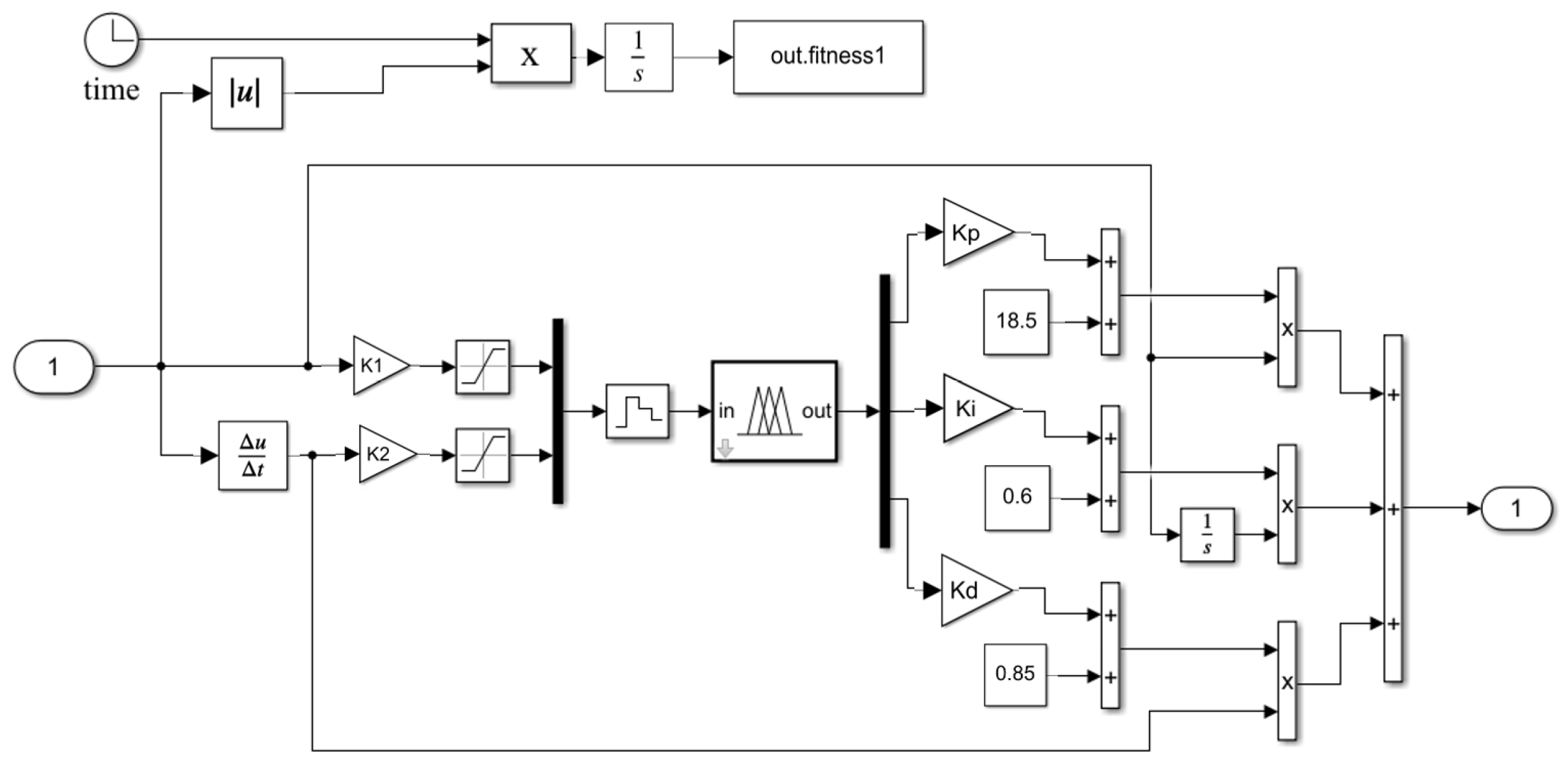
4.1. Fuzzy-PID Controller Design

The core of the Fuzzy-PID controller comprises both the traditional PID control algorithm and fuzzy inference mechanisms. As illustrated in Figure 6, the PID control algorithm is expressed as:
u ( t ) = K p   e ( t ) + K i o t e ( t ) + K d d e ( t ) d ( t )
where Kp is the proportional coefficient, Ki is the integration coefficient, Kd is the differential coefficient, and e(t) is the real-time displacement deviation.
The self-tuning Fuzzy-PID controller uses the error (E) and the rate of change of the error (EC) as inputs, meeting the requirement for real-time adjustment of PID parameters based on E and EC. By integrating fuzzy theory, the PID parameters are online corrected to meet the varying requirements for controller parameters under different E and EC conditions, thereby improving the control performance of the controlled system.
This paper designs a hydraulic system Fuzzy-PID flow control block diagram as shown in Figure 6, adopting a self-tuning Fuzzy-PID controller structure. The electro-hydraulic proportional flow valve controller consists of a fuzzy controller and a PID controller. The inputs to the fuzzy controller are the rotation angle error E (with gain KE) and the error rate EC (with gain KEC). The outputs are the three correction parameters for the PID controller: ΔKp, ΔKi, and ΔKd [29]. The three input parameters of the PID controller are determined according to the following equation, where Kp0, Ki0, and Kd0 represent the initial values of the proportional gain, integral gain, and derivative gain of the PID controller, respectively, and are determined empirically.
K p = K p 0 + Δ K p K i = K i 0 + Δ K i K d = K d 0 + Δ K d

4.2. Establishment and Fuzzification of Fuzzy Controller Input and Output Variables

Based on the above analysis, the MATLAB (R2022a) setting window was first opened to set E and EC as input ports and Kp, Ki, and Kd as output ports.
After setting the input port quantification factors KE and KEC and the output ports Kp, Ki, and Kd, the range of each domain is determined. The [−3, 3] domain (e.g., in Mamdani controllers) maps to 7 linguistic levels, adapting to various plants and eliminating unit-dependency issues. Set input end and deviation change rate theory domain [−3, 3], set output end, Kp, Ki, Kd theory domains, respectively, [−3, 3], set Kp, Ki, Kd theory domains [−0.3, 0.3], [−0.06, 0.06], [−0.3, 0.3], the fuzzy subset of its control is set to negative, negative, negative, zero, zero, center, center, in logical reasoning rules: PB, PM, PS, ZO, NS, NM, NB; membership function selection for a more sensitive trimf type [30,31].

4.3. Determination of Membership Functions and Establishment of Fuzzy Control Rules

Due to its small memory usage and simple computational characteristics, the triangular membership function is particularly suitable for fuzzy control with online parameter adjustment. It is commonly used in fuzzy control systems, especially when real-time parameter modification is required, offering high efficiency. Therefore, this paper selects the triangle to describe the fuzzy sets of each variable.
Based on expert experience, the control rule table is established [32,33]. The quantization factors KE and KEC are set within the ranges of [−3, 3] and [−3, 3], respectively. The output variables Kp, Ki, and Kd are selected, and the fuzzy rules for the system are established as shown in Table 3.

4.4. PSO-Optimized Fuzzy-PID Control for Flow Valve

The performance of a fuzzy controller is limited by the complexity of rule and membership function design, as well as empirical requirements. The PSO algorithm, an intelligent optimization algorithm with few parameters and fast convergence, is suitable for optimizing Fuzzy-PID controller parameters. In PSO, particle movement is influenced by both its own and the group’s best solutions, with the fitness function measuring the distance between the particle and the solution. The nonlinear and time-varying characteristics of the hydraulic system align well with PSO’s global search capability. PSO, through multi-particle collaboration, avoids local optima, outperforming traditional single-point optimization methods.
The velocity of each particle is represented by xv and yv, respectively, indicating the velocity along the X and Y axes. The position update of the particle is realized by the calculation of the current position and velocity information, and each particle knows the best value obtained in the search process and the corresponding XY coordinate. This information reflects the search process of the particle, and each particle also knows the best value in the solution space. Each search agent adjusts its position according to the following information: (1) current position (x, y); (2) current speed (xv, yv); (3) the value of the current position of the historical individual; (4) the value of the current preferred solution of the group [34].
The velocity and position of each particle are updated according to Equations (28) and (29), respectively.
v i k + 1 = v i k + c 1 · r a n d 1 · ( p b e s t i s i k ) + c 2 · r a n d 2 · ( g b e s t s i k )
s i k + 1 = s i k + v i k + 1
During the PSO, where v i k is the current velocity of the particle i at the k iteration, v i k + 1 is the new velocity of particle i in the generation k iteration, c 1 is the individual learning factor; c 2 is the group learning factor, r a n d 1,2 is a random number between 0 and 1, s i k is the current position of particle i in the generation k iteration, s i k + 1 is the new position of particle i in the generation k iteration, p b e s t i is the optimal position of the individual in generation i, and gbest is the group optimal position. During the PSO process, each particle updates its current position using vector operations, as illustrated in Figure 7.

4.4.1. Selection of Objective Function

In parameter optimization, the objective function is used to evaluate the system performance, selecting different objective functions to reflect different performance dimensions. The ideal objective function should be easy to calculate and accurately evaluate the system performance. The ITAE criterion was chosen as the objective function because of its small transient response oscillation and good selectivity for parameters. Equation (30) is a mathematical expression of the integral time absolute error (ITAE) criterion: an objective function of this integral form, expressing the cumulative value of the absolute error over the whole time period from beginning to end. Typically, a smaller ITAE indicates that the controller can eliminate errors more quickly, reduce overshoot and oscillations, and maintain very low steady-state error over long-term operation, thus improving both transient response and steady-state accuracy.
I T A E = 0 t e ( t )   d t

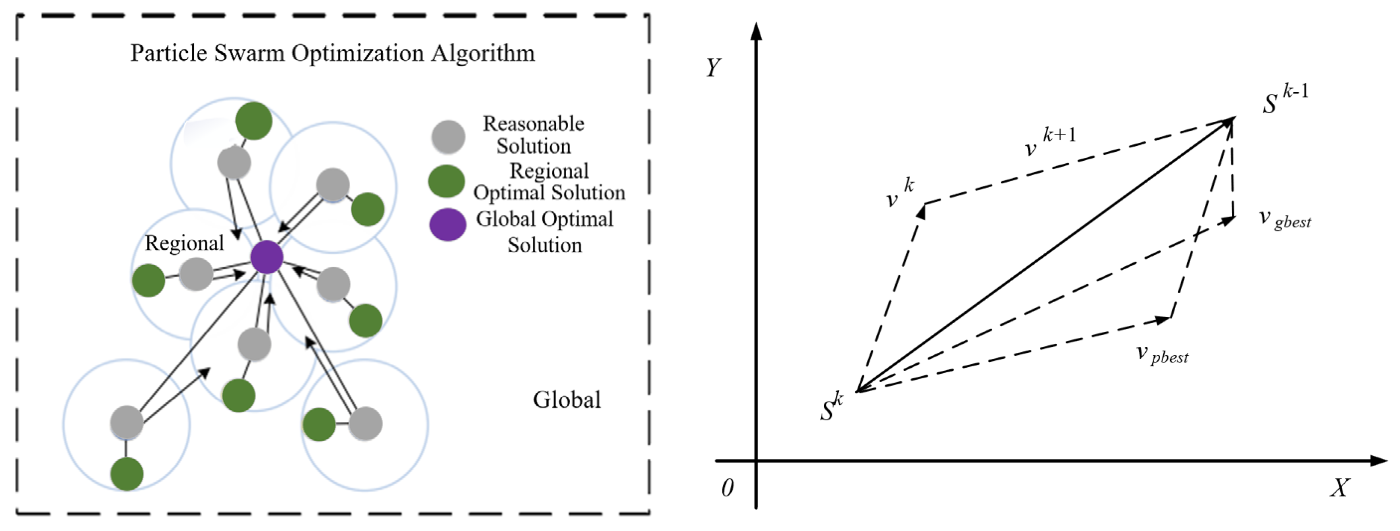
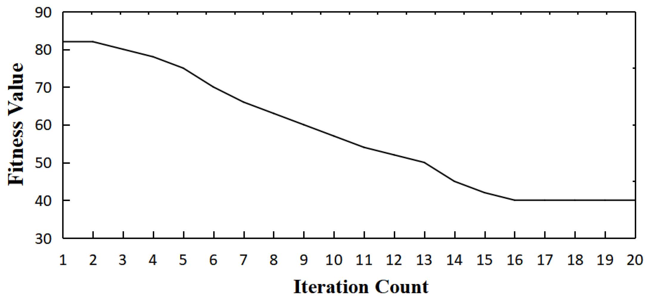
4.4.2. PSO Parameter Settings and Iteration Process

The parameters of the PSO algorithm are shown in Table 4. Increasing the inertia weight nnn enhances the global search capability, and its typical range is from 0.9 to 1.2. In this study, a value of 0.9 was selected. The learning factors c1 and c2 generally range from 0 to 4, and 2 is selected in this paper. For general engineering problems, the PSO sizes are usually between 20 and 100, and increasing the size can improve the convergence and find the global optimal solution but requires a corresponding increase in the number of iterations. When the scale increases to a certain extent, the improvement of convergence is no longer obvious, and the scale N is chosen to be 50. The dimension D represents the number of unknowns in the problem, and this paper involves five parameters, KE, KEC, Kp, Ki, and Kd, so the dimension is set to 5. Too small a number of iterations t will result in unstable output, while too many will increase the computation time. In the optimization process, the number of iterations is adjusted according to practical considerations, with 20 iterations set in this study.

5. Simulation Analysis and Experimental Study of Electro-Hydraulic Proportional Flow Valve Flow Control

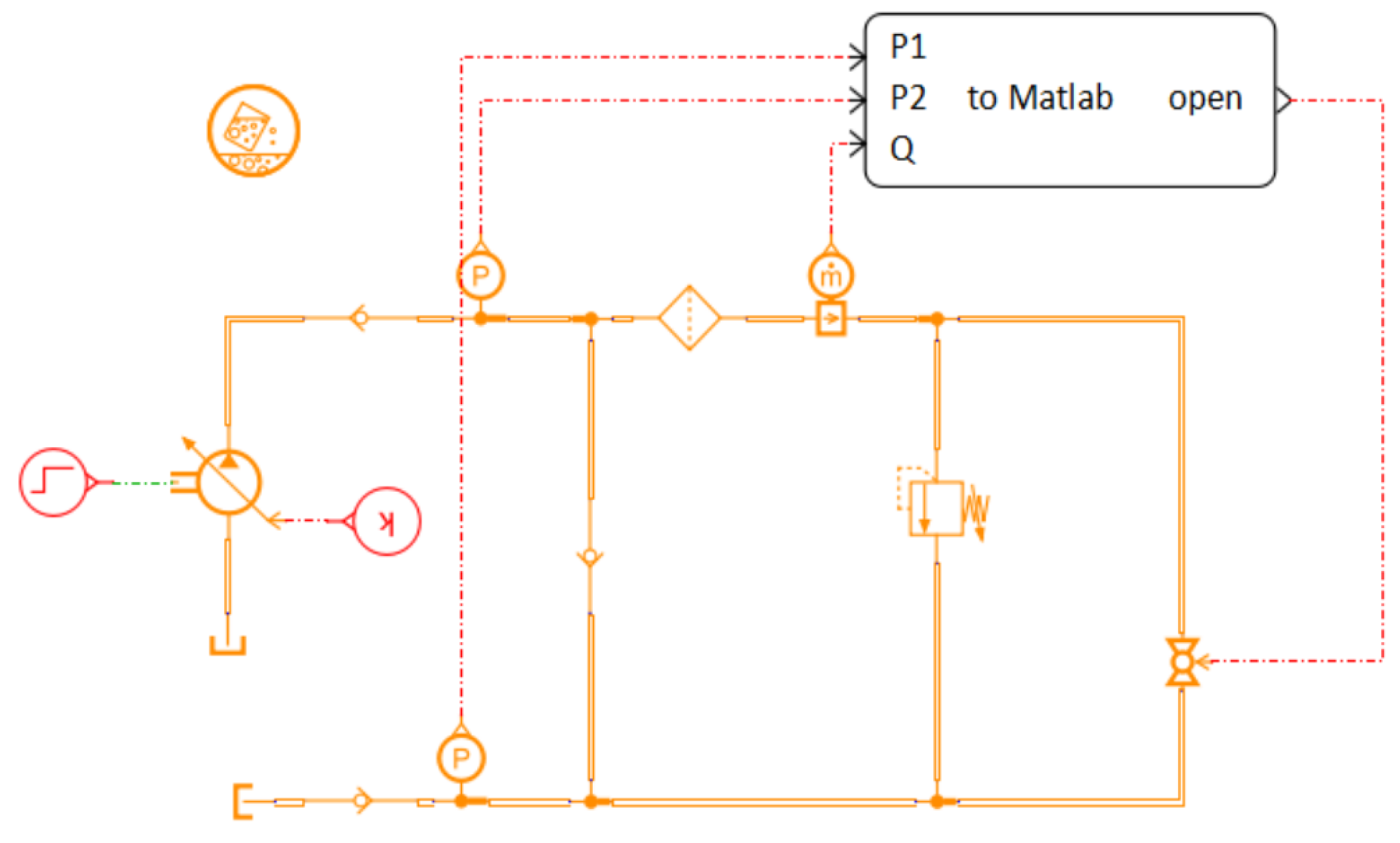
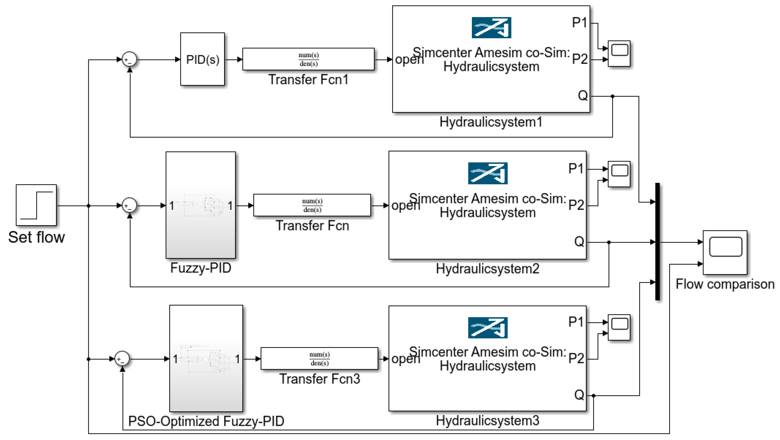
5.1. Establishment of Hydraulic Control System Co-Simulation Model

Based on the approximate relationship between hydraulic pipeline flow and the input angle of the ball valve, a flow control model of the hydraulic system is established using a hydraulic tester. This model takes the ball valve angle as input and the flow signal from the system flow meter as output, adjusting the flow in the pipeline by varying the input angle.
Due to the nonlinear characteristics of the hydraulic system, it is difficult to describe the relationship between input and output with a single mathematical equation or transfer function. Therefore, the AMEsim hydraulic simulation module is used to build a simulation model of the system as a substitute for a theoretically derived mathematical model. In AMEsim, an interface is created to pass the valve angle as an input variable to the ball valve module, and the flow meter output is connected to the system output interface, thereby linking the pipeline flow to the ball valve input angle.
The simulation model is built based on the hydraulic test circuit diagram shown in Figure 1. A variable power hydraulic pump is used to simulate the tractor part, providing flow and pressure to the test pipeline. The hydraulic pipeline modeling of the test circuit is shown in Figure 8.
After completing the construction of the hydraulic pipeline model, a MATLAB/Simulink co-simulation interface module is added to transfer the system’s input and output variables to MATLAB. The AMEsim hydraulic simulation model is used as the transfer function of the hydraulic part and, together with the transfer function of the electro-hydraulic proportional flow valve actuator, serves as the controlled object in the subsequent MATLAB simulation analysis for flow control. By configuring the components and parameters of the “Hydraulic Control System Simulation Model” shown in Figure 8, the hydraulic system simulation model is completed.

5.2. Simulation Model of Electro-Hydraulic Proportional Flow Control System

The electro-hydraulic proportional control system simulation model includes a comparison of three control methods. Figure 9 and Figure 10 show the simulation models of the Fuzzy-PID controller and the PSO-optimized Fuzzy-PID controller, respectively.
Figure 11 illustrates the variation curve of the performance index ITAE during the PSO simulation iteration process. In this study, the fitness value was multiplied by a gain factor of 10−4 to facilitate data observation. By analyzing the iterative process, it can be observed that the parameters approach their optimal values after 16 iterations. Upon reaching the maximum number of iterations, the performance index requirement is satisfied, and the iteration process concludes. The optimized parameter values are presented in Table 5.
By iteratively optimizing the fuzzy factors, the PSO-optimized Fuzzy-PID tuning results are obtained, as shown in Table 5. The optimized parameter values are Ke = 0.12, Kec = 0.006, with a corresponding fitness value of ITAE = 0.041.

5.3. Stability and Robustness Analysis of the PSO-Optimized Fuzzy-PID Controller

To verify the stability and robustness of the PSO-optimized Fuzzy-PID controller in the flow control task, the controller was implemented using the MATLAB/Simulink interface, and 20 independent simulation experiments based on Figure 11 were conducted. The mean and standard deviation of the 20 ITAE values were calculated, and a one-way analysis of variance (one-way ANOVA) was performed to assess the significance of differences among the simulation runs.
As shown in Table 6, results from 20 independent simulation experiments indicate that the PSO-optimized Fuzzy-PID controller exhibits good robustness: the average ITAE is 0.0410 (σ ≈ 0.00045), and the ANOVA test yields a p-value of 0.212 (>0.05), confirming its stability in the flow control of the hydraulic power tester and providing a basis for subsequent field experiments.
This study uses AMEsim and MATLAB/Simulink for co-simulation of the flow control system. The control system simulation model is built in MATLAB/Simulink. Based on the controller parameters designed in this study, a controller simulation model is constructed in Simulink, and the derived transfer function along with the SimulinkCosim co-simulation interface module is integrated into the control model. These two submodules are then encapsulated. The final electro-hydraulic proportional flow control system simulation model based on the YYSCT-250-3 is shown in Figure 12.
Relevant system parameters are input into the simulation model and configured sequentially according to the system model parameters of the low-flow, medium-flow, and high-flow circuits. A step signal is applied to the input flow for simulation testing.

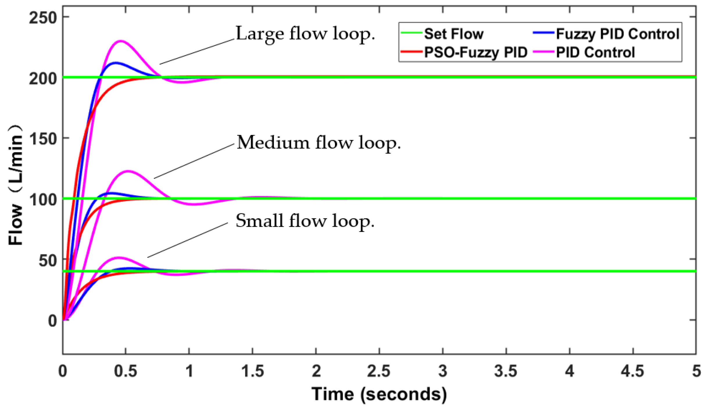
5.4. Analysis of Hydraulic Simulation Results for Different Flow Rate Loop Sections

During the low-flow simulation in AMESim, the hydraulic pipe diameter was set to 15 mm, the maximum flow rate of the hydraulic pump was set to 100 L/min, and the rotational speed was 2000 r/min. After running the Simulink simulation, the step response curve of the flow rate was obtained as shown in Figure 13, and the corresponding performance indicators are listed in Table 5. From the step response of the low-flow circuit (Figure 13), it can be seen that the traditional PID control exhibits the fastest response time (0.48 s) but comes with the largest overshoot. Based on this, the Fuzzy-PID control reduces the overshoot to 6.2%, with a slightly increased response time of 0.51 s, and effectively suppresses oscillations. Further employing PSO-optimized Fuzzy-PID results in an almost negligible overshoot (only 0.1%) and a response time of 0.68 s. Although the differences in response times among the three control methods are minimal—indicating a similar sensitivity of the low-flow system to the control strategies—in terms of steady-state performance, the traditional PID achieves a steady-state error of less than 2%, slightly outperforming the Fuzzy-PID. The Fuzzy-PID accelerates convergence and reduces oscillations, while the PSO-Fuzzy-PID further suppresses overshoot and minimizes system impact, achieving the best overall performance.
For the medium-flow simulation, the pipe diameter in AMESim was set to 25 mm, and the hydraulic pump’s maximum flow rate was set to 166 L/min. After running the Simulink simulation, the step response curve was obtained (Figure 13), with corresponding performance indicators listed in Table 5. The step response shows that traditional PID control results in the largest overshoot and the longest response time. With the addition of a fuzzy controller, the maximum overshoot is significantly reduced. After PSO, the Fuzzy-PID overshoot is nearly eliminated. Although the response times of the three control methods are similar, indicating no significant difference in sensitivity, the steady-state error of traditional PID is less than 2%, slightly outperforming Fuzzy-PID. However, Fuzzy-PID effectively suppresses oscillations and improves steady-state convergence speed. The PSO-optimized Fuzzy-PID further reduces overshoot and system impact, achieving superior overall performance. In summary, for the medium-flow control loop, the PSO-optimized Fuzzy-PID offers the shortest settling time and minimal overshoot, outperforming both traditional PID and standard Fuzzy-PID control.
For the high-flow simulation, the loop pipe diameter in AMESim was set to 32 mm, and the hydraulic pump’s maximum flow rate was 250 L/min. After running the Simulink simulation, the step response curve (Figure 13) was obtained, and system performance indicators are summarized in Table 7. Results show that traditional PID control produces the largest overshoot and longest response time. Introducing a fuzzy controller significantly reduces the overshoot, while PSO-optimized Fuzzy-PID nearly eliminates it. Response times among the three methods are similar, indicating negligible difference in responsiveness for high-flow systems. Although traditional PID achieves a steady-state error below 2%, slightly better than Fuzzy-PID, the latter improves convergence speed and suppresses oscillations. PSO-Fuzzy-PID further minimizes overshoot and reduces system impact. Overall, for high-flow control loops, the PSO-optimized Fuzzy-PID achieves the best performance in terms of settling time and overshoot, outperforming both traditional PID and standard Fuzzy-PID.

5.5. Test and Result Analysis

To verify the accuracy of the simulation model, an experiment was conducted in April 2024 at the Nanjing Agricultural University-Baima Teaching and Research Base in Lishui District, Nanjing, on the “YYSCT-250-3”. The test machines used included various specifications of flow tractors such as the Huanghai-Jinma YEX504, Ruiwo F1200, and Fubotian-2604.
The set flow rates were set to 40 L/100 L/200 L/min, with the tractor hydraulic pump’s rated speed at 2000 r/min, the relief valve set to 35 MPa, and using 46# hydraulic oil. Under normal temperature conditions, the flow control program of the test instrument was activated. After setting the target flow rate, the flow in the hydraulic test circuit was initially zero, and the electro-hydraulic proportional valve spool was fully open. The tractor then started to supply oil to the test circuit, and the flow regulation test began. As the hydraulic pump supplied oil, the flow was controlled by precisely adjusting the ball valve opening. Flow characteristic tests of the hydraulic system were conducted, with three sets of tests repeated to reduce errors. The average values were taken, and the test data were plotted into response curves, as shown in Figure 14, Figure 15 and Figure 16.
To verify the performance of the designed PSO-optimized Fuzzy-PID controller in flow control, the Fuzzy-PID control algorithm is implemented in MATLAB/Simulink and connected to the PLC programmable controller via LabVIEW. The optimized control parameters are input into the YYSCT-250-3 hydraulic system test equipment for real-time adjustment and performance testing. The field and equipment of this experiment are shown in Figure 17.

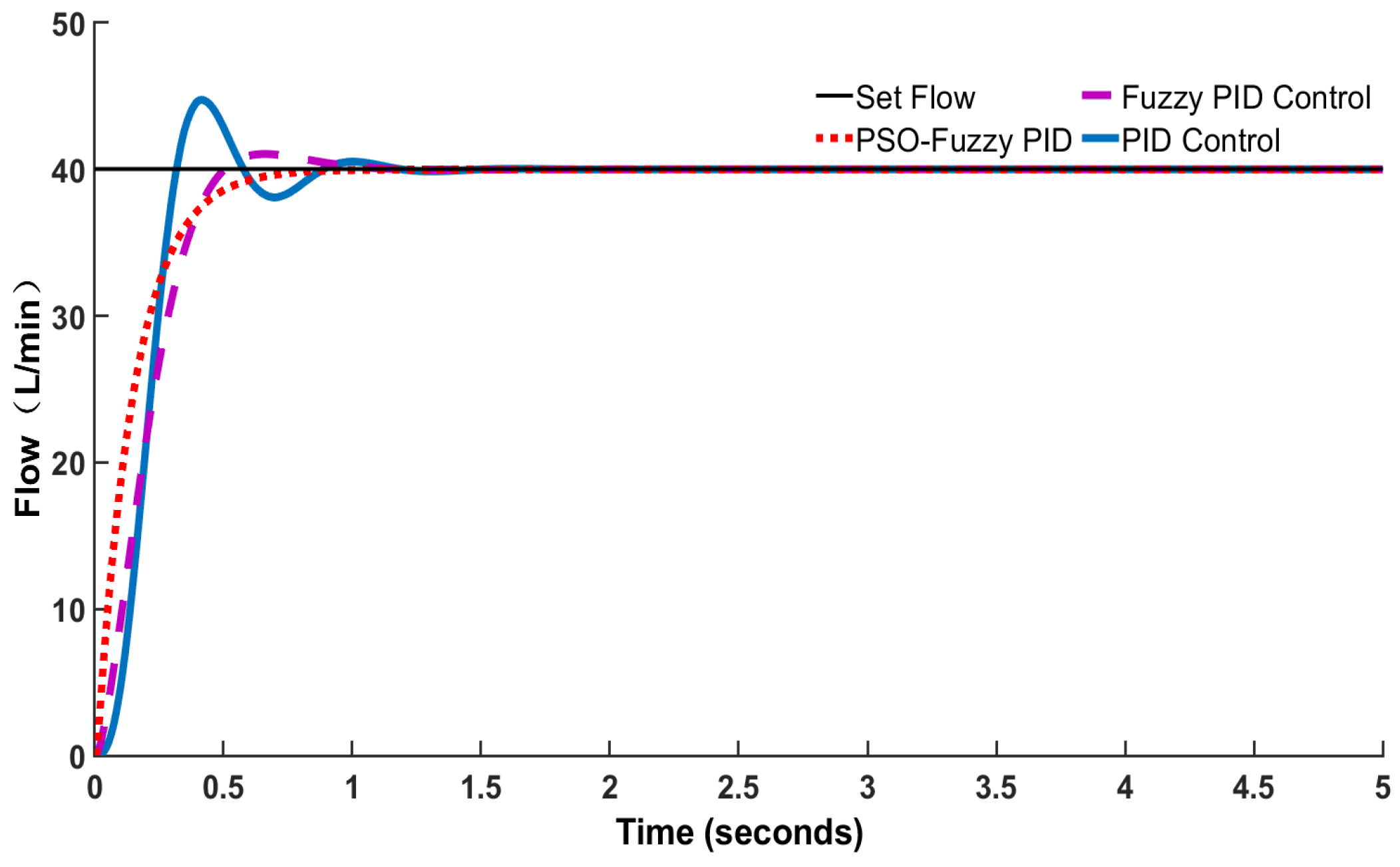
5.5.1. Low Flow Rate YYSCT-250-3 Test

To verify the precise flow control at 40 L/min for the YYSCT-250-3, the flow was accurately controlled by adjusting the opening of the proportional flow ball valve. The system flow control response curve is shown in Figure 14, and the corresponding data are presented in Table 8.
As shown in Figure 14, experiments were conducted on the low-flow 40 L/min circuit model using three control methods: PID, Fuzzy-PID, and PSO-optimized Fuzzy-PID. The results indicate that the performance of the PSO-optimized fuzzy control is superior to the first two methods. Overall, the controller’s performance in flow control meets the target requirements.
As shown in Figure 14, the system response time for all three control methods under the low flow of 40 L/min is 0.3 s. With PID control, the settling time is 1 s and the overshoot is 9.0%. With Fuzzy-PID control, the settling time is 0.88 s and the overshoot is 2.4%. Under PSO-optimized Fuzzy-PID, the settling time is 0.8 s and the overshoot is almost 0. The overshoot of the PSO-optimized Fuzzy-PID control is minimal, not exceeding 1.0%, with a steady-state error within ±1.0%. The PSO-optimized Fuzzy-PID controller achieves the target flow control requirements. Overall, unlike the simulation experiment, the PID and Fuzzy-PID responses exhibit larger overshoots, likely due to flow fluctuations caused by various influencing factors in the hydraulic system. From the steady-state time perspective, the designed controller meets the expected target, reaching the set flow value within 1 s. During the low-flow 40 L/min test, the flow stabilized at 40.4 L/min, its absolute steady-state error is within ±0.5 L/min of the set target value, and the relative error is 1.0% of the target value. To optimize its parameters, the PSO algorithm rapidly converges to the optimal Fuzzy-PID settings in just a few iterations, thereby greatly reducing both the system’s overshoot and steady-state error. This demonstrates that, in control scenarios with strong nonlinearities and time-varying characteristics (such as hydraulic systems), the adaptive parameter-tuning capability of the proposed algorithm offers significant advantages.
Based on the data in Table 8, the improvement of PSO-Fuzzy-PID over traditional methods is calculated as follows: Overshoot Elimination: PSO-Fuzzy-PID achieves nearly 100% overshoot elimination across low, medium, and high flow rates, while Fuzzy-PID only eliminates 73.3%, 53.8%, and 21.2%, respectively. Settling Time Optimization: Compared to PID, PSO reduces settling time by 20–41% (e.g., for low flow rates: 1 s → 0.8 s, a 20% improvement). Compared to Fuzzy-PID, it further optimizes settling time by 9.1–13.3% (e.g., for medium flow rates: 0.9 s → 0.78 s, a 13.3% improvement). Although the PSO-Fuzzy-PID controller demonstrates excellent performance across all flow rates, the improvement in overshoot reduction in medium- and high-flow conditions is not as pronounced as at low flow. This may be attributed to factors such as increased system friction, pipeline volume effects, and oil temperature variations under high-flow conditions.

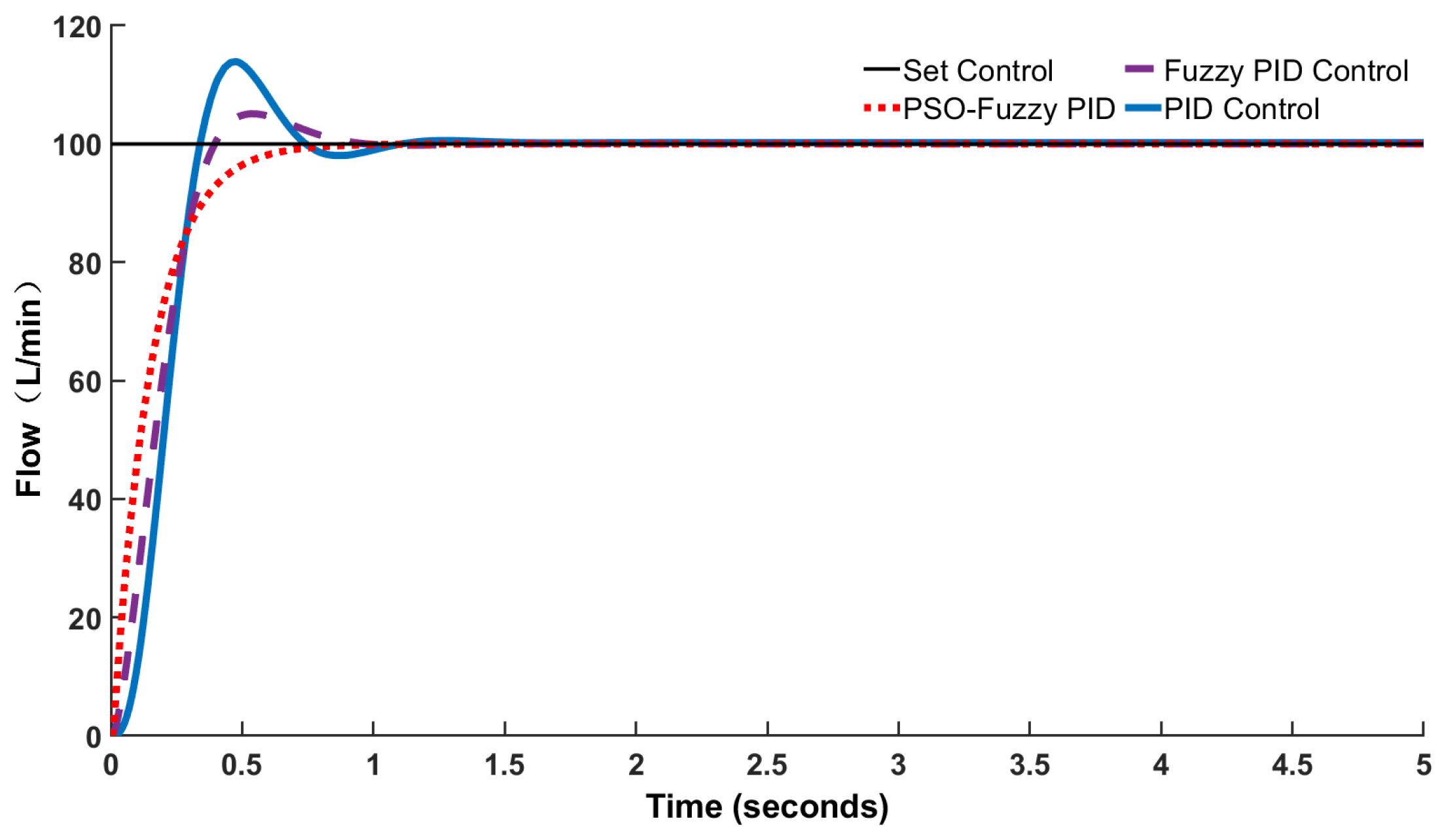
5.5.2. Medium Flow Rate YYSCT-250-3 Test

To verify the precise flow control of the YYSCT-250-3 at a flow rate of 100 L/min, the system controls the opening of the proportional flow valve. The system’s flow control response curve can be seen in Figure 15 and Table 8.
As shown in Figure 15, experiments were conducted on the medium-flow 100 L/min circuit model using three control methods: PID, Fuzzy-PID, and PSO-optimized Fuzzy-PID. The results indicate that the performance of the PSO-optimized fuzzy control is superior to the first two methods. Overall, the controller’s performance in flow control meets the target requirements.
As shown in Figure 15, for the medium flow rate of 100 L/min, the system response time under all control methods is 0.32 s. Under PID control, the settling time is 1.1 s with an overshoot of 16.9%. Under Fuzzy-PID control, the settling time is 0.9 s, and the response time is 0.8 s with an overshoot of 7.8%. With PSO-optimized Fuzzy-PID, the settling time is 0.78 s, and the overshoot is nearly 0%. The PSO-optimized Fuzzy-PID controller effectively meets the target requirements for flow regulation. The system ultimately stabilizes at 100.5 L/min, its absolute steady-state error is within ±0.5 L/min of the set target value, and the relative error is 0.5% of the target value.
Through the global optimization of KE, KEC, and PID parameters using the particle swarm optimization (PSO) algorithm, the limitations of traditional fuzzy control relying on expert experience are overcome. As shown in Figure 8, PSO converges within 16 iterations, demonstrating its rapid optimization capability.
Flow-Pressure Coupling Suppression: The flow equation of the hydraulic system is [35]:
Q = C d   A 2 Δ P ρ
Optimize the PID parameters (ΔKp, ΔKi, ΔKd) (reference Equation (27)) to improve the dynamic performance. The proportional valve opening A is adjusted to compensate for the influence of ΔP fluctuations and reduce the oscillation caused by the intrinsic lag ring of the electro-hydraulic proportional valve. The intrinsic retardation of the electro-hydraulic proportional valve causes a small jitter in the PID/Fuzzy-PID curve in Figure 14, Figure 15 and Figure 16. After PSO, the Kp gain was increased to 9.16 (see Table 4), which enhanced the system stiffness, and the test results verified the smoothness improvement of the curve after PSO.
Under medium-flow conditions, due to the strong coupling between flow and pressure, significant nonlinear fluctuations persist in the system, especially during sudden load changes and switching processes, where secondary oscillations are likely to occur. To address this issue, future research may incorporate state observation or robust control strategies to further suppress coupling disturbances and improve overshoot mitigation.

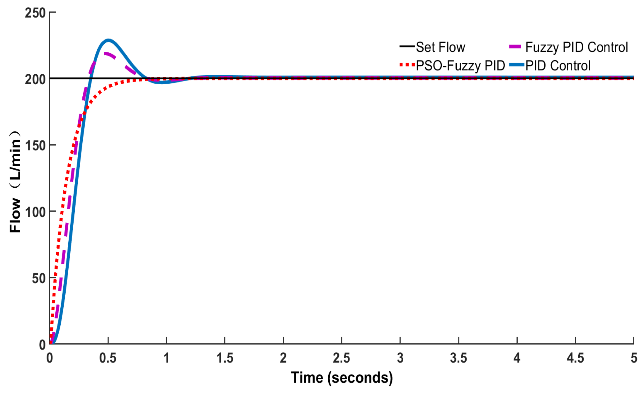
5.5.3. High Flow Rate YYSCT-250-3 Test

To verify the precise flow control of the YYSCT-250-3 at a flow rate of 200 L/min, the system controls the opening of the proportional flow valve. The system’s flow control response curve can be seen in Figure 16 and Table 8.
Experiments were conducted on the high-flow 200 L/min circuit model using three control methods: PID, Fuzzy-PID, and PSO-optimized Fuzzy-PID. The results indicate that the performance of the PSO-optimized Fuzzy control is superior to the first two methods. Overall, the controller’s performance in flow control meets the target requirements.
As shown in Figure 16, the flow control test results indicate that for the high flow of 200 L/min, the system response time for all three methods is 0.35 s. With PID control, the settling time is 1.4 s and the overshoot is 14.6%; with Fuzzy-PID control, the settling time is 0.92 s and the overshoot is 11.5%; with PSO-optimized Fuzzy-PID, the settling time is 0.82 s and the overshoot is nearly 0. The PSO-optimized Fuzzy-PID controller achieves flow regulation that meets the target requirements. Overall, unlike the simulation experiment, the PID and Fuzzy-PID responses exhibit smaller overshoots, likely due to the hydraulic system itself eliminating some friction power losses, which reduces flow fluctuations. From the perspective of settling time, the designed controller meets the expected target, reaching the set flow range within 1.00 s. During the test, the flow stabilized at 200.5 L/min, its absolute steady-state error is within ±0.5 L/min of the set target value, and the relative error is 0.5% of the target value. Hydraulic Shock Suppression: According to the fluid mechanics momentum equation:
F = ρ   Q   v
PSO causes the overshoot to approach zero (as shown in Table 8), directly reducing the instantaneous flow impact force. In the experiment, the PSO curve exhibits no overshoot, reducing hydraulic shock by more than 90% compared to PID.
Compared with the simulation of Figure 13, Figure 14, Figure 15 and Figure 16, the steady state error of the PSO controller was 0.5 L/min under a low flow (40 L/min) and high flow (200 L/min), proving that its robust performance was better in the full flow range, while the traditional PID increased from 9.0% to 14.6% when the flow increased, with poor adaptability. PSO reduces the steady state time by 30–40%, reduces the pressure loss caused by frequent valve adjustment. Taking the 200 L/min working condition as an example, PSO brings the system into the steady state in 0.58 s (1.4 s → 0.82 s in advance) and reduces the energy consumption of hydraulic output by Equation (1). A reduction in energy consumption of over 30% can be achieved, demonstrating that the fast-converging control strategy offers a significant advantage in minimizing energy losses.
These results indicate that the PSO-Fuzzy-PID controller maintains steady-state flow control errors within ±0.5 L/min across the full operating range (40–200 L/min), demonstrating strong robustness against system nonlinearities and parameter fluctuations.

6. Conclusions

This study addresses the nonlinear coupling and dynamic hysteresis challenges in flow control of a tractor multi-channel hydraulic tester (YYSCT-250-3) by constructing a hydraulic system simulation model in AMESim and introducing a PSO-optimized Fuzzy-PID controller. Through a tri-level innovation path of model correction, algorithm optimization, and platform validation, both theoretical and engineering breakthroughs were achieved. The main conclusions are as follows:
(1)
This work is the first to systematically analyze the nonlinear coupling mechanism between hydraulic damping and friction effects and to establish a modified transfer function model incorporating spool resistance torque and fluid pulsation dynamics. Experimental results show that the prediction error converges within ±0.5%, significantly improving modeling accuracy under complex conditions. The model reveals the mechanical–fluid interaction mechanism from a multi-physics coupling perspective and provides a theoretical foundation for high-precision flow regulation.
(2)
The PSO-based multi-objective fitness function within the AMESim–MATLAB co-simulation framework overcomes the empirical dependency of traditional Fuzzy-PID control. Tests show that, under 40 L/min conditions, the system overshoot is reduced by 78.9% compared to segmented PID [3] (from 1.42% to 0.3%), and the number of convergence iterations is 37% lower than that of GA-optimized control [18] (from 32 to 20), demonstrating the algorithm’s global optimization efficiency and control robustness in complex hydraulic systems.
(3)
The hardware-in-the-loop (HIL) testing platform based on the OPC protocol resolves the parameter transfer gap between simulation and real-vehicle conditions. Under steady-state flow conditions (40–200 L/min), the absolute control error is within ±0.5 L/min (relative error ≤ ±1.0%), showing superior accuracy and consistency over traditional Fuzzy-PID methods [7]. The modular plug-and-play design offers a standardized technical interface for the intelligent upgrade of agricultural hydraulic systems.
(4)
The current model does not account for viscosity changes under extreme oil temperatures (<−20 °C or >60 °C). Future work will incorporate temperature–viscosity compensation to enhance environmental adaptability. In addition, advanced control methods such as adaptive robust control (ARC) and model predictive control (MPC) will be introduced to improve real-time control accuracy and expand the theoretical and technical scope of intelligent control in agricultural hydraulics. In addition, online self-tuning mechanisms and machine-vision-based flow detection will be introduced to establish a more intelligent, closed-loop adaptive control system.
(5)
In terms of scalability, future work will explore coordinated control strategies for multi-channel hydraulic circuits to mitigate power oscillations caused by uneven flow distribution. The proposed friction–flow coupling model shows potential for lifespan prediction, expanding the theoretical perspective of condition monitoring. The PSO-Fuzzy-PID approach also demonstrates good transferability to scenarios such as combine harvester drive control and precision irrigation distribution. Future research will integrate emerging technologies such as digital twins and edge computing to promote the evolution of agricultural hydraulic systems toward adaptive, high-reliability, and low-energy solutions.

Author Contributions

Conceptualization, Q.L., Z.L. and X.B.; methodology, Q.L. and X.D.; software, Q.L.; validation, Z.L. and X.B.; investigation, Z.L. and X.B.; resources, X.D.; writing—original draft preparation, Y.L. and Q.L.; writing—review and editing, Q.L., X.D. and Z.L.; visualization, Q.L. and X.B.; supervision, Z.L. and X.B.; project administration, X.B. and Z.L. All authors have read and agreed to the published version of the manuscript.

Funding

The National Key Research and Development Plan (grant number: 2022YFD2001202) and research and development project of tractor multiplex hydraulic output device performance parameter testing equipment (grant number: NJ2022-16).

Institutional Review Board Statement

Not applicable.

Data Availability Statement

The data presented in this study are available on demand from the corresponding authors at xiaotingdeng@njau.edu.cn or 17852036730@163.com (Q.L.).

Acknowledgments

The authors thank the anonymous reviewers for providing critical comments and suggestions that improved the manuscript.

Conflicts of Interest

The authors declare no conflicts of interest.

References

  1. Gu, L.C.; Qi, Z.L.; Li, J.B. Application study of fuzzy and PID control in flow control of hydraulic power source at variable speed. Mech. Des. Manuf. 2021, 4, 29–33. [Google Scholar]
  2. Ma, F.; Miao, J.; Fan, G.; Li, S.; Ye, F.; Luo, Y. Design and Experiment of a Profiling Soil Covering Device for Sugarcane Planter in Hilly Areas. Trans. Chin. Soc. Agric. Eng. 2025, X, 1–11. [Google Scholar]
  3. Wang, H.; Liu, Y.H.; Zhou, L.M.; Zhou, H.Y.; Niu, K.; Xu, M.H. Design and Experiment of a Segmented PID Control System for Fertilizer Flow in a Fertilizer Seeder. Trans. Chin. Soc. Agric. Mach. 2023, 54, 32–40+94. [Google Scholar]
  4. Ketelsen, S.; Padovani, D.; Andersen, T.O.; Ebbesen, M.K.; Schmidt, L. Classification and Review of Pump-Controlled Differential Cylinder Drives. Energies 2019, 12, 1293. [Google Scholar] [CrossRef]
  5. Sun, C.; Dong, X.; Wang, M.; Li, J. Sliding mode control of electro-hydraulic position servo system based on adaptive reaching law. Appl. Sci. 2022, 12, 6897. [Google Scholar] [CrossRef]
  6. Li, M.S.; Ye, J.; Xie, B.; Yang, S.; Zeng, B.G.; Liu, J. Design and Experiment of a Hydraulic Proportional Flow Valve for Tractor Hydraulic Chassis. Trans. Chin. Soc. Agric. Mach. 2018, 49, 397–403. [Google Scholar]
  7. Mao, W.; Ji, Z.K.; Wei, H.L.; Peng, X.W. Application Research of Fuzzy PID Composite Control in Electro-Hydraulic Proportional Servo Systems. Hydraul. Pneum. 2019, 1, 95–99. [Google Scholar] [CrossRef]
  8. Li, H.T.; Li, W.; Hu, C.Y.; Wang, R.; Luo, K.K. Fault-Tolerant Control Method for Electro-Hydraulic Servo Systems Based on Fuzzy PID Signal Compensation. Gas Turbine Technol. 2021, 34, 15–22. [Google Scholar]
  9. Li, W.J.; Gong, G.F.; Liu, J.; Zhang, Y.K.; Yang, H.Y. Simulation of Train Braking Electro-Hydraulic System Based on High-Frequency Solenoid Valve Pressure Control. J. Cent. South Univ. (Sci. Technol.) 2020, 51, 340–348. [Google Scholar]
  10. Wrat, G.; Bhola, M.; Ranjan, P.; Mishra, S.K.; Das, J. Energy Saving and Fuzzy-PID Position Control of Electro-Hydraulic System by Leakage Compensation through Proportional Flow Control Valve. ISA Trans. 2020, 101, 269–280. [Google Scholar] [CrossRef]
  11. Huang, K.W.; Qin, X.P.; Zhan, J.; She, Y.; Wu, F.; Miao, D.; Yang, S.M. Fuzzy PID Control for Hydraulic Steering of Heavy-Duty AGV. Hydraul. Pneum. 2021, 45, 108–115. [Google Scholar]
  12. Chen, Z.G.; Hu, S.C.; Li, X.Q. Variable amplitude hydraulic control system based on fuzzy PID. Chin. Hydraul. Pneum. 2021, 45, 156–162. [Google Scholar]
  13. Luo, Q.Z.; An, A.M.; Zhang, H.C.; Meng, F.C. Non-Linear Performance Analysis and Voltage Control of MFC Based on Feedforward Fuzzy Logic PID Strategy. J. Cent. South Univ. 2019, 26, 3359–3371. [Google Scholar] [CrossRef]
  14. Ghasemi, A.; Azimi, M.M. Adaptive fuzzy PID control based on nonlinear disturbance observer for quadrotor. J. Vib. Control 2022, 29, 965–2977. [Google Scholar] [CrossRef]
  15. Peng, H.; Wang, J.Z.; Shen, W.; Li, D.Y. Application of Dual Fuzzy Control with Compensation Factor in Electro-Hydraulic Servo Valve-Controlled Asymmetric Cylinder Systems. J. Mech. Eng. 2017, 53, 184–192. [Google Scholar] [CrossRef]
  16. Niu, B. Research on Performance of Intelligent Control Valve Based on PID Fuzzy Control. Supervisor: Fan, Y.G. Master’s Thesis, Xi’an Shiyou University, Xi’an, China, 2023. [Google Scholar]
  17. Hou, Y.; Fan, J. Research on Hydraulic Drive Active Heaving Compensation Predictive Control Based on Neural Network PID Control. J. Mach. Tools Hydraul. 2020, 48, 145–148. [Google Scholar]
  18. Mounce, S.; Shepherd, W.; Ostojin, S.; Abdel-Aal, M.; Schellart, A.; Shucksmith, J.; Tait, S. Optimisation of a fuzzy logic-based local real-time control system for mitigation of sewer flooding using genetic algorithms. J. Hydroinform. 2020, 22, 281–295. [Google Scholar] [CrossRef]
  19. Liu, B. Speed Tracking Control of Vehicle Hydraulic Transmission Based on IPSO Fuzzy PID. Automot. Maint. 2024, 3, 26–28. [Google Scholar]
  20. Shen, Z.; Cheng, H.; Li, H. Design of an Electro-hydraulic Proportional Position Control System for Sugarcane Topper Cutter Based on Fuzzy PID Method. Trans. Chin. Soc. Agric. Mach. 2025, Online First, 1–13. Available online: http://kns.cnki.net/kcms/detail/11.1964.s.20241010.1555.002.html (accessed on 22 February 2025).
  21. Li, Y.; Li, Y.Z. Fuzzy PID parameter optimization of valve controlled hydraulic cylinder based on improved ant colony algorithm. Mach. Des. Manuf. 2018, 7, 143–146. [Google Scholar]
  22. Wu, C.W.; Zhu, Y.C.; Gao, Q. Fuzzy adaptive PID control of pneumatic position servo system using high-speed on/off valves. Chin. Hydraul. Pneum. 2021, 45, 47–53. [Google Scholar]
  23. Zhang, J.; Zhang, C.Y.; Zhang, S.H.; Hu, Z.Q. Multi-Cylinder Position Synchronization Control Based on Mean Coupling. Hydraul. Pneum. 2021, 2, 50–55. [Google Scholar]
  24. Zhao, S. Research on the hydraulic servo flow control method based on LADRC. J. Eng. Mech. Control 2022, 20, 45–52. [Google Scholar]
  25. Yao, Y.F.; Chen, X.G.; Ji, C.; Chen, J.C.; Zhang, H.; Pan, F. Design and Experiment of a Monomer Actuator for Corn Precision Planters Based on Fuzzy PID Control. Trans. Chin. Soc. Agric. Eng. 2022, 38, 12–21. [Google Scholar]
  26. Qi, W.; Yang, B.; Chao, Y. Research on Synchronization of Hydraulic Fracturing Pumps Based on Fuzzy RBF. Mach. Tool Hydraul. 2023, 51, 44–50. [Google Scholar]
  27. Mao, W.; Zheng, Y.S.; Wang, D.R.; Sun, J.; Dou, X.Z. Analysis of Flow Characteristics of V-Ball Valves with Different Cone Angles. Hydraul. Pneum. 2021, 45, 165–171. [Google Scholar]
  28. Yi, P.F.; Ma, S.W.; Zhang, J.P.; Li, Y.F.; Ren, L. Transient Flow Characteristics Analysis of PVC Ball Valves Based on Dynamic Mesh Simulation. J. Water Resour. Archit. Eng. 2022, 20, 130–135+141. [Google Scholar]
  29. Xiao, M.H.; Ma, Y.; Wang, C.; Chen, J.; Zhu, Y.; Bartos, P.; Geng, G. Design and Experiment of Fuzzy-PID Based Tillage Depth Control System for a Self-Propelled Electric Tiller. Int. J. Agric. Biol. Eng. 2023, 16, 116–125. [Google Scholar] [CrossRef]
  30. Chen, L.J.; Peng, Z.Q.; Sun, J.Q.; Gao, W.; Hua, Z.; Ai, C. Adaptive Compensation Control for Nonlinear Position of Pilot-Operated Electro-Hydraulic Proportional Valves. Hydraul. Pneum. 2021, 45, 64–71. [Google Scholar]
  31. Solovjev, D.S. Improving the electroplating coating uniformity based on fuzzy control of the setting value using the combined defuzzification method with the presence of stochastic influences. Solid State Phenom. 2022, 6653, 112–120. [Google Scholar] [CrossRef]
  32. Chen, J.; Lu, Q.; Bai, J.; Xu, X.; Yao, Y.; Fang, W. A Temperature Control Method for Microaccelerometer Chips Based on Genetic Algorithm and Fuzzy PID Control. Micromachines 2021, 12, 1511. [Google Scholar] [CrossRef] [PubMed]
  33. Shi, C.D.; Zhang, Y.C. Research on speed control of hydraulic drive spindle based on fuzzy adaptive PID controller. Chin. J. Eng. Mach. 2020, 18, 516–520. [Google Scholar]
  34. Tian, M.; Platinum, B.; Li, J.H.Q. A fertilization control system based on genetic algorithm. J. Agric. Eng. 2021, 37, 21–30. [Google Scholar]
  35. Hao, W.; Jiyun, Z.; Chao, C.; Yunfei, W.; He, Z. Modeling and simulation analysis of a novel proportional water flow valve with a digital pilot stage. Proc. Inst. Mech. Eng. Part E 2024, 09544089231224325. [Google Scholar] [CrossRef]
Figure 1. Overall structure diagram of YYSCT-250-3. (a) Front sectional view (1—High-flow Hydraulic Test System. 2—Medium-flow Hydraulic Test System. 3—Low-flow Hydraulic Test System. 4—Measurement Unit. 5—Communication Cable. 6—All-in-One Industrial Control–Display. 7—Control and Display Unit. 8—Printer. 9—Enclosure/Casing. 10—Boss/Protrusion. 11—Toolbox) (b) Bottom sectional view (12, 19—Temperature Sensor. 13, 18—Pressure Sensor. 14, 17—Quick-connect Coupling. 15—Return Hose. 16—Inlet Hose. 20—Filter. 21, 25—Check Valve. 22—Flow Meter. 23—High-pressure Hydraulic Hose. 24—Relief Valve. 26—Electro-hydraulic Proportional Flow Valve).
Agriculture 15 01190 g001
Figure 2. The composition of testing equipment for the performance parameters of the tractor multi-way hydraulic output device.
Agriculture 15 01190 g002
Figure 3. Hydraulic test loop.
Agriculture 15 01190 g003
Figure 4. Internal structure of electric actuator. (1—Protective Cover. 2—Gear Assembly. 3—Slot. 4—Worm Gear. 5—Terminal Block. 6—Wire Lock. 7—Turbine Shaft. 8—Turbine Shaft Stopper. 9—Turbine. 10—Motor Assembly. 11—Roto. 12—Dial. 13—Pointer/Needle. 14—Glass Panel. 15—Switch Stopper).
Agriculture 15 01190 g004
Figure 5. Mathematical model of electro-hydraulic proportional flow valve system.
Agriculture 15 01190 g005
Figure 6. Schematic diagram of Fuzzy-PID hydraulic flow controller.
Agriculture 15 01190 g006
Figure 7. Schematic diagram of particle position adjustment.
Agriculture 15 01190 g007
Figure 8. Simulation model of hydraulic control system.
Agriculture 15 01190 g008
Figure 9. Fuzzy-PID simulation model.
Agriculture 15 01190 g009
Figure 10. PSO-optimized Fuzzy-PID simulation model.
Agriculture 15 01190 g010
Figure 11. Change curve of ITAE performance index of PSO algorithm.
Agriculture 15 01190 g011
Figure 12. Simulation model of electro-hydraulic proportional flow control system.
Agriculture 15 01190 g012
Figure 13. Simulated Step Responses of Control Loops under Different Flow Conditions.
Agriculture 15 01190 g013
Figure 14. Circuit test results at 40 L/min.
Agriculture 15 01190 g014
Figure 15. Loop test result at 100 L/min.
Agriculture 15 01190 g015
Figure 16. Loop test result at 200 L/min.
Agriculture 15 01190 g016
Figure 17. Test the site and the device.
Agriculture 15 01190 g017
Table 1. Main structural and performance parameters of YYSCT-250-3.
ParametersUnitsValues
Overall dimensions (door closed state)mm1200 × 700 × 1800
Supply voltageHz220 VAC/50 Hz
Weightkg350
Low flowL/min~100
Medium flowL/min~166
High flowL/min~250
Hydraulic input/output port pressureMPa(0~40) MPa, accuracy: 0.5% FS
Hydraulic oil temperature°C(0~150) °C, accuracy: ±0.5 °C
Table 2. Parameters of NT-5 and NT-10 electric actuators.
ParametersNT-5-50 N·mNT-10-100 N·m
Motor shaft moment of inertia (J)6.01 × 10⁻⁴ kg·m21.2 × 10−3 kg·m2
Friction coefficient (f)1.4 × 10⁻⁵ N·m·s/rad2.8 × 10−5 N·m·s/rad
Stator resistance (Ra)2.12 Ω1.56 Ω
Gear reduction ratio (i)100100
Motor back-EMF constant (Ke)0.126 V/rad0.25 V/rad
Electrical inductance (La)4.2 mH4.52 mH
Torque constant (Km)15.9 N·m/A8.7 N·m/A
Moment of inertia of the load ball valve (Jz)1.0 × 10⁻⁵ kg·m27.7 × 10−5 kg·m2
Table 3. Fuzzy rules for Kp, Ki, and Kd.
EC\ENBNMNSZ0PSPMPB
NBZO/NB/NSZO/NB/NSPS/NB/NSPS/NM/NSPM/ZO/NSPM/ZO/NSPM/ZO/NS
NMZO/NB/NSZO/NB/NSPS/NM/NSPS/NM/NSPM/NS/NSPM/ZO/NSPM/ZO/NS
NSZO/NM/NSZO/NM/NSPS/ZO/NSPS/NS/NSPM/ZO/ZOPM/PS/ZOPM/PS/ZO
Z0ZO/ZO/NSZO/NS/NSPS/ZO/ZOPS/ZO/ZOPM/PS/ZOPM/PM/PSPM/PM/PS
PSPS/NM/NSPS/NS/NSPS/ZO/ZOPS/PS/ZOPM/PS/ZOPM/PM/PSPM/PB/PS
PMPS/NM/PSPS/ZO/PSPM/PS/PSPM/PM/PSPB/PM/PSPB/PB/PSPB/PB/PS
PBPS/ZO/PSPS/ZO/PMPM/ZO/PMPM/PM/PMPB/PB/PMPB/PB/PBPB/PB/PM
Table 4. Particle swarm algorithm parameter setting.
Namenc1, c2NDt
Parameter0.9250520
Table 5. Fuzzy-PID tuning results of particle swarm optimization.
Parameter-Tuning ResultsKeKecKpKiKdITAE
PSO-Optimized Parameter Values0.120.0069.160.080.50.041
Table 6. ITAE data statistics.
Number of Runs (i)ITAE(i)Number of Runs (i)ITAE(i)Number of Runs (i)ITAE(i)Number of Runs (i)ITAE(i)
10.041760.0408110.0404160.0409
20.040970.0414120.0412170.0411
30.040580.0406130.0408180.0406
40.041190.0410140.0408190.0415
50.0413100.0407150.0413200.0410
Table 7. Performance Indicators of Loop Step Response under Different Flow Rates.
CategoryOvershootResponse TimeSettling Time
Low-flow loopPID17.6%0.48 s1.64 s
Fuzzy-PID6.2%0.51 s0.85 s
PSO-optimized Fuzzy-PID0.1%0.68 s0.76 s
Medium-flow loopPID22.3%0.62 s1.71 s
Fuzzy-PID5.8%0.43 s0.78 s
PSO-optimized Fuzzy-PID0.1%0.58 s0.69 s
High-flow loop13.00%0.54 s1.16 s13.00%
4.00%0.46 s0.69 s4.00%
0.06%0.44 s0.51 s0.06%
Table 8. Test results of low, medium, and high flow rates.
Flow Specifications
(L/min)
Controlling MeansOvershoot (%)Settling Time (s)Response Time (s)
Low flow 40 L/minPID9.01.000.30
Fuzzy-PID2.40.880.30
PSO-Fuzzy PID00.800.30
Medium flow
100 L/min
PID16.91.100.32
Fuzzy-PID7.80.900.32
PSO-Fuzzy PID00.780.32
High flow
200 L/min
PID14.61.400.35
Fuzzy-PID11.50.920.35
PSO-Fuzzy PID00.820.35
Disclaimer/Publisher’s Note: The statements, opinions and data contained in all publications are solely those of the individual author(s) and contributor(s) and not of MDPI and/or the editor(s). MDPI and/or the editor(s) disclaim responsibility for any injury to people or property resulting from any ideas, methods, instructions or products referred to in the content.

