
E-CLIP: An Enhanced CLIP-Based Visual Language Model for Fruit Detection and Recognition

Abstract
1. Introduction
- (1)
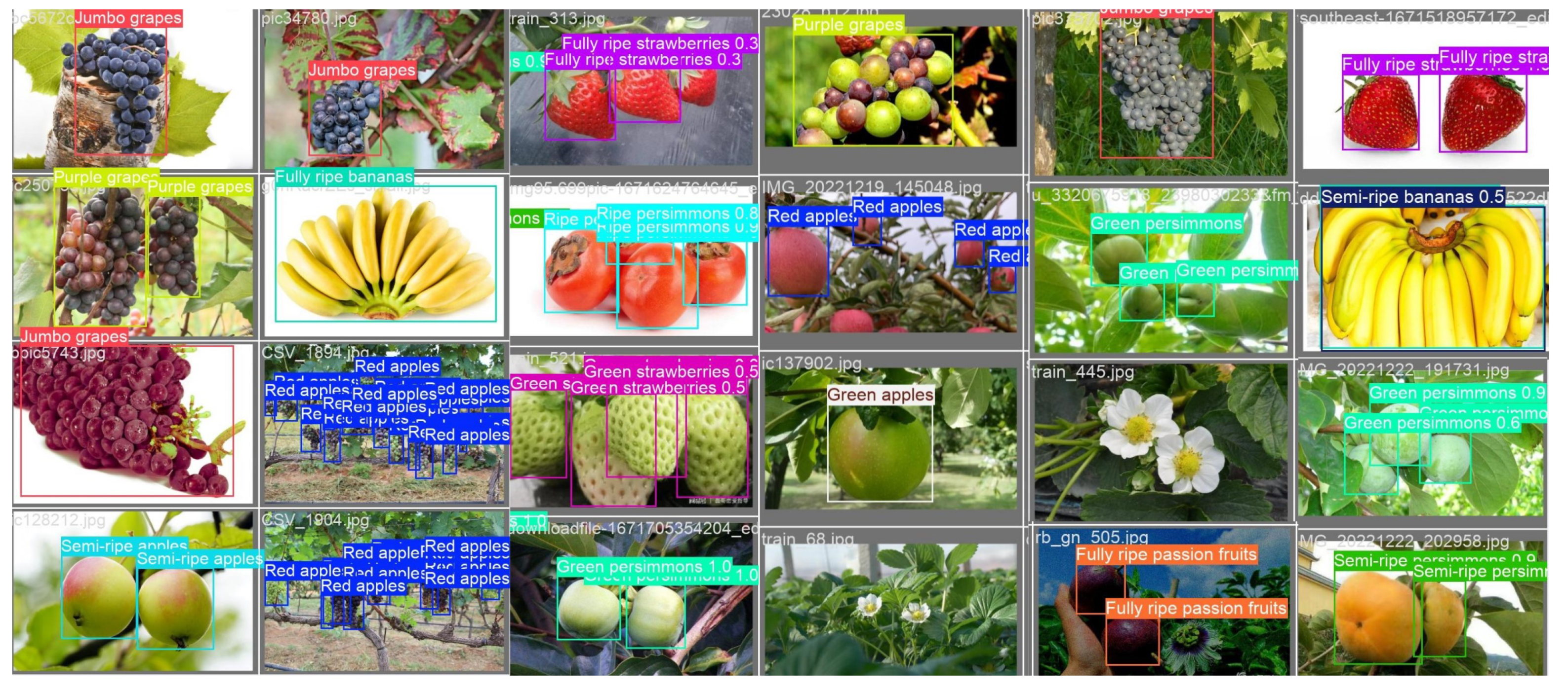
- Multimodal Fruit Dataset: A multimodal dataset was constructed specifically designed for fruit recognition in agricultural robotics. The dataset comprises 6770 real-world orchard images spanning 12 fruit categories, with 7 categories annotated at three maturity levels (unripe, semi-ripe, and ripe). Additionally, we generated 100 natural language queries using Qwen-7B to establish semantic alignments between visual features and textual descriptions. This dataset facilitates both fine-grained maturity detection and open-set recognition, enabling systems to adapt to dynamic picking instructions.
- (2)
- Natural Language Instruction Module: An input module for natural language instructions has been developed, integrating a language model parser, enabling robots to perform complex tasks based on natural language commands (through text or voice inputs). This enhances operational flexibility and user interaction. Furthermore, this language input will be combined with image data to improve the accuracy of subsequent fruit detection and recognition. The method significantly lowers the technical threshold for agricultural robots, aiding in their wider adoption and utilization in fruit picking.
- (3)
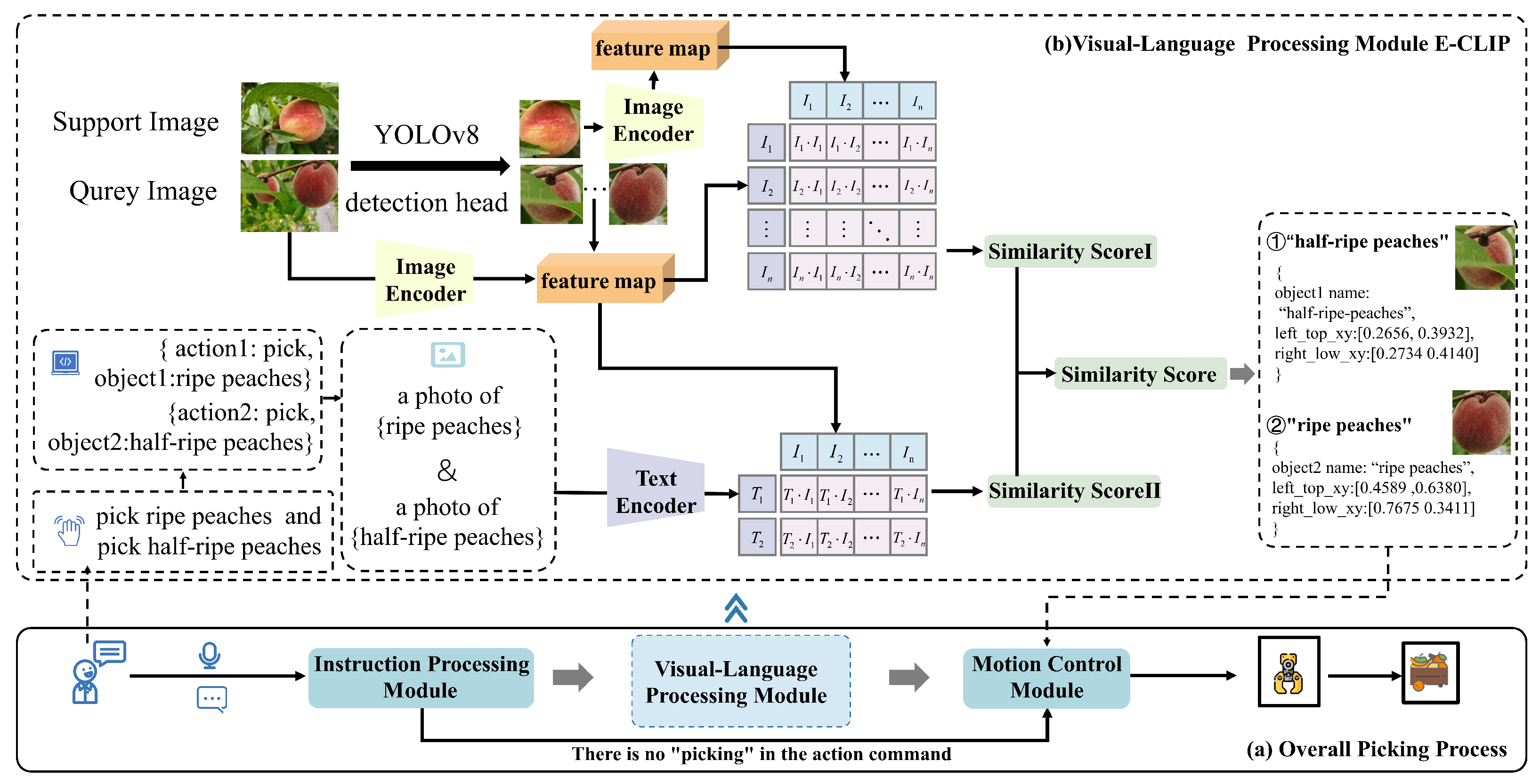
- Enhanced CLIP Model Architecture: An enhanced CLIP model architecture has been proposed, modifying the original CLIP framework by incorporating three key components: a YOLO detection head, an image–image contrastive learning branch, and an image–text contrastive learning branch. The YOLO detection head is used to detect fruit regions within images; the image–image contrastive learning branch focuses on identifying similarities between different fruit images, enhancing the model’s recognition capability in scenarios with scarce data and complex environmental conditions. The image-to-text contrastive learning branch contrasts structured natural language instructions with images, learning the relationship between instructions and fruit features. This not only enhances the model’s understanding of task requirements but also leverages the mapping between text and images in zero-shot scenarios, thus improving the model’s generalization ability.
2. Materials and Methods
2.1. Multimodal Dataset
2.1.1. Dataset Construction
- Field capture: Use a high-resolution camera to capture clear images under various occlusion conditions (such as slight occlusion/moderate occlusion/heavy occlusion).
- Open data sources: Additional images of mangoes and tomatoes were sourced from open-access repositories to enhance dataset diversity.
2.1.2. Dataset Preprocessing
2.2. The Overall Framework of Fruit-Picking System
- (1)
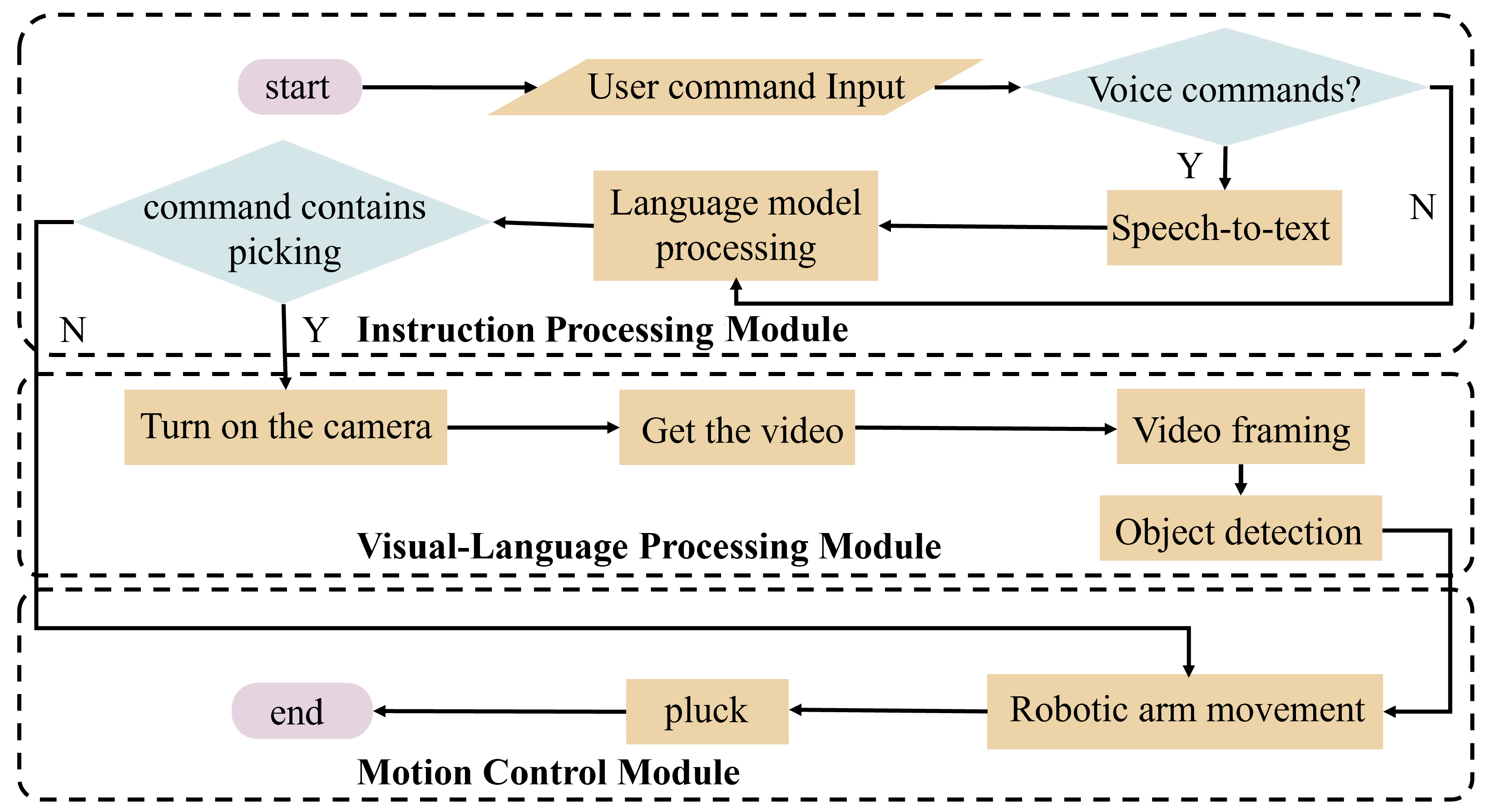
- Instruction Processing Module: Processes natural language commands describing picking requirements.
- (2)
- Visual Language Processing Module: Analyzes multimodal information including vision and text data, through the VLM for context understanding and object recognition, then outputs the 2D bounding box coordinates of detected targets.
- (3)
- Motion Control Module: Generates actionable motor commands by fusing prior perception results.
2.2.1. Instruction Processing Module
2.2.2. Visual Language Processing Module
- (1)
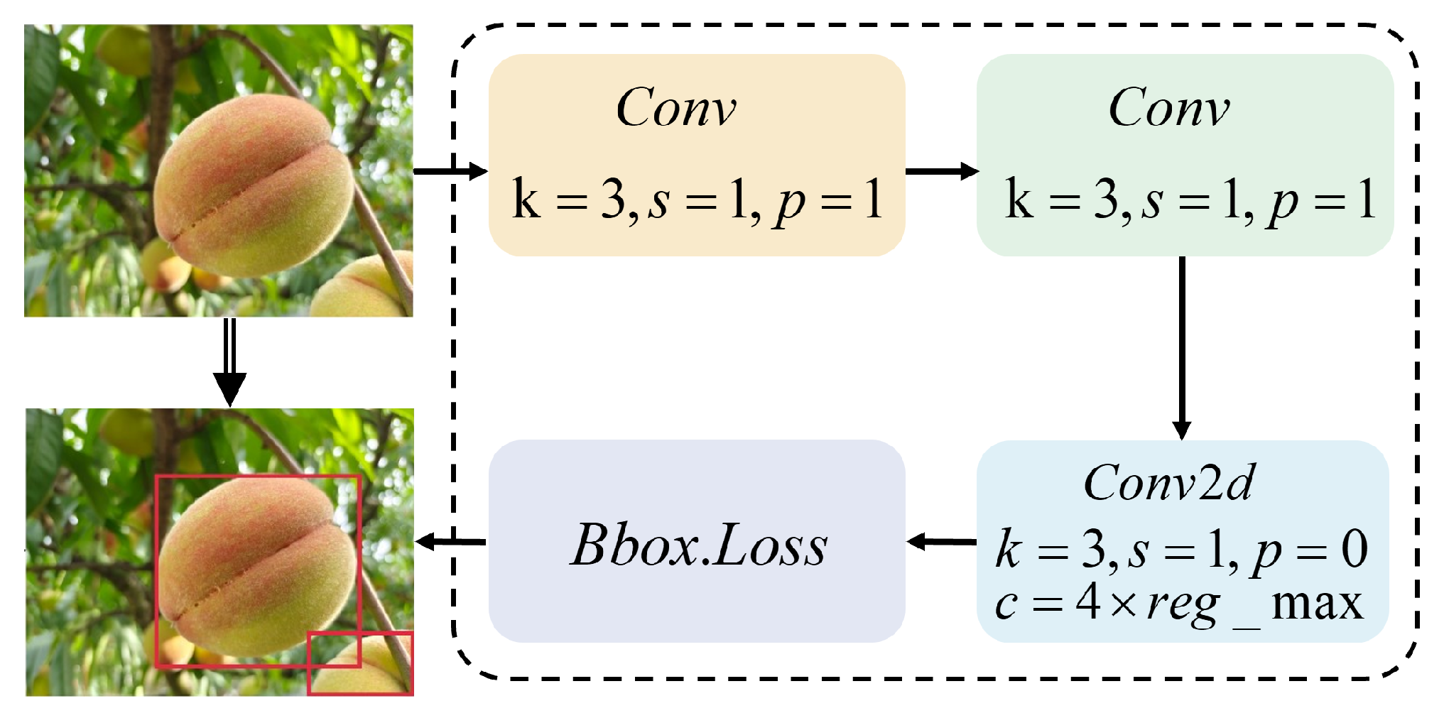
- YOLOv8 Detection Head
- (2)
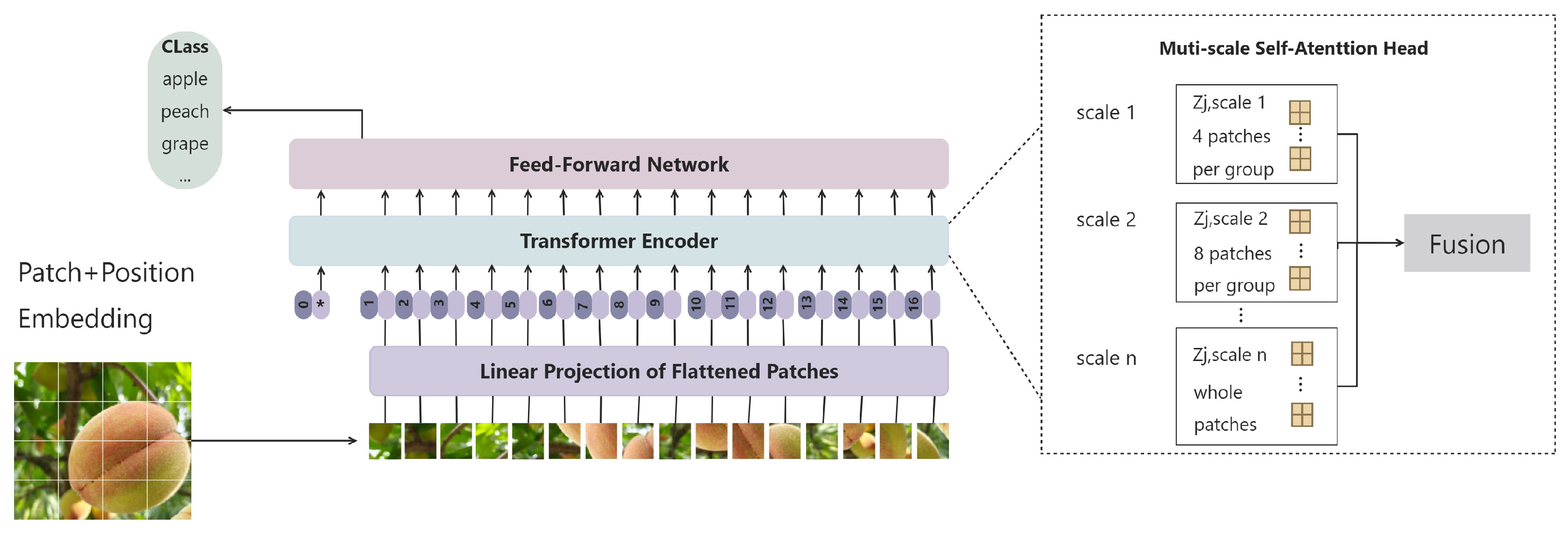
- Image Encoder
- (3)
- Text Encoder
- (4)
- Loss Function
- (5)
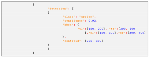
- Fruit Detection Output
2.3. Experimental Setup
2.3.1. Implementation Details
2.3.2. Hyperparameter Settings
2.3.3. Evaluation Metrics
- (1)
- Precision (P), reflecting the proportion of true positive samples among all detected positives, is defined as:where denotes correctly identified positive samples, and represents false positives.
- (2)
- Recall (R), which quantifies the fraction of actual positives accurately predicted by the model, is given by:where indicates negatives incorrectly classified as such.
- (3)
- The F1 score, calculated as the harmonic mean of precision and recall, provides a balanced assessment:
- (4)
- Average precision (AP) measures localization accuracy by determining the area under the precision–recall curve. Mean average precision (mAP), an aggregate measure across all classes, reflects overall detection performance:where N is the total number of classes.
- (5)
- Intersection over union (IoU), indicating spatial overlap between predicted and ground-truth bounding boxes, is expressed as:where A and B represent the areas of the predicted and ground-truth bounding boxes, respectively.
- (6)
- GFLOPs, measuring computational complexity, are calculated as follows:where H and W are the height and width of the output feature map, respectively.
- (7)
- Parameters quantify the total trainable parameters within the model, particularly convolutional layers, via the following:where K is the convolutional kernel size, is the number of input channels, and is the number of output channels.
- (8)
- Finally, FPS, representing inference speed, is given by the following:where N is the total number of processed frames, and is the total inference time in seconds.
3. Results and Discussion
3.1. Language Model Comparison
3.2. Visual Language Model Evaluation
3.2.1. Model Performance Comparision
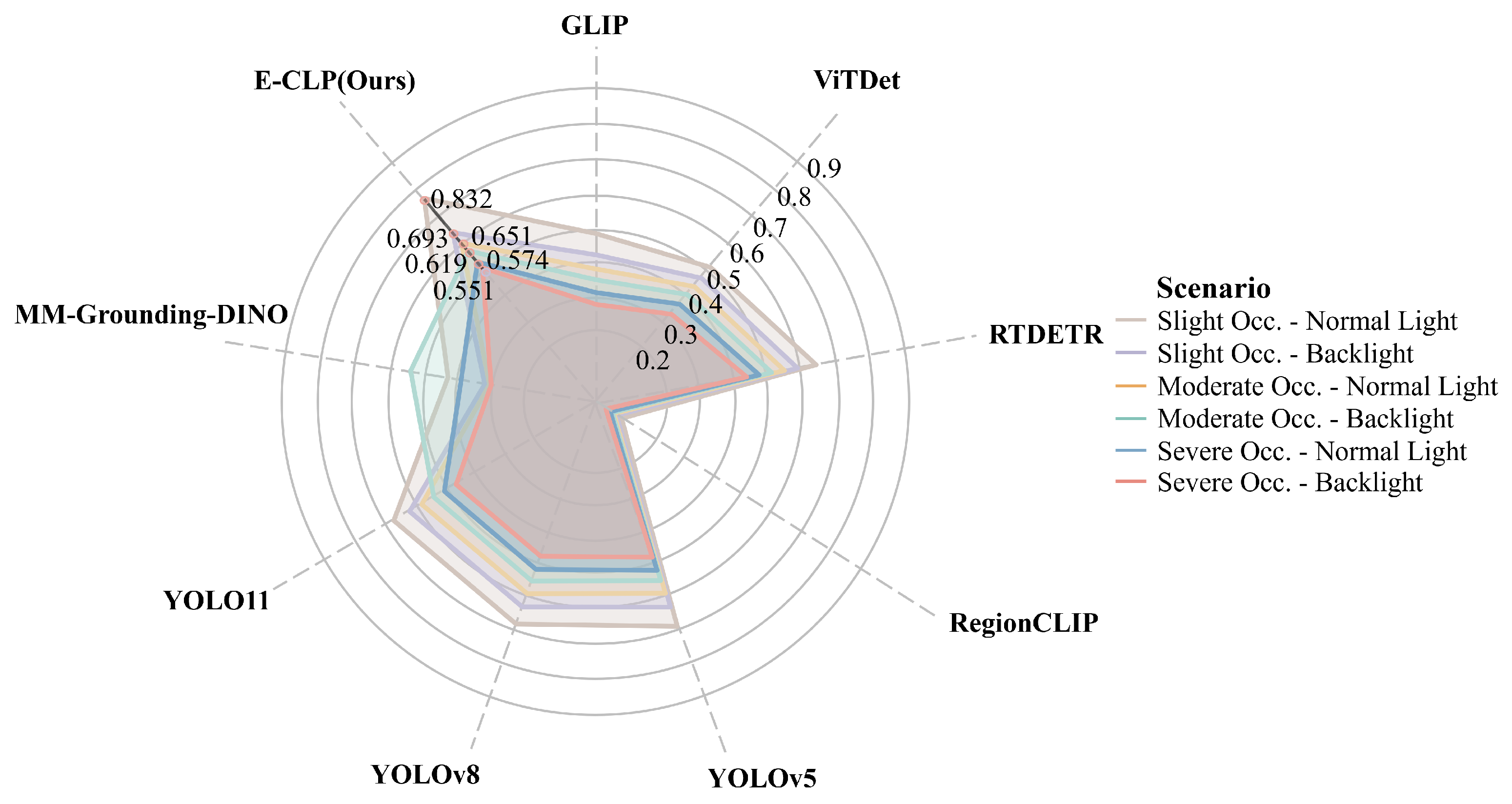
3.2.2. Robustness Assessment
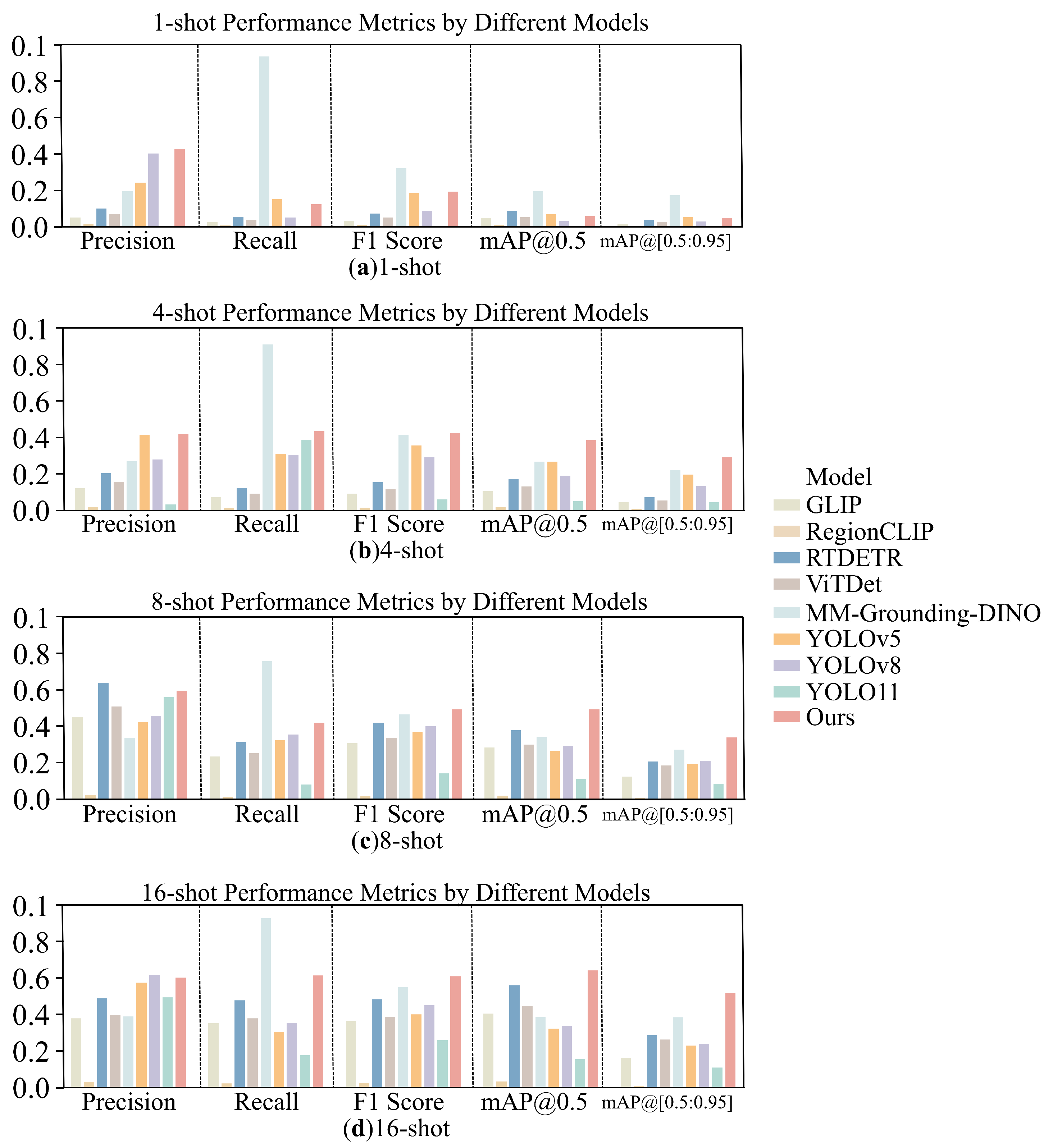
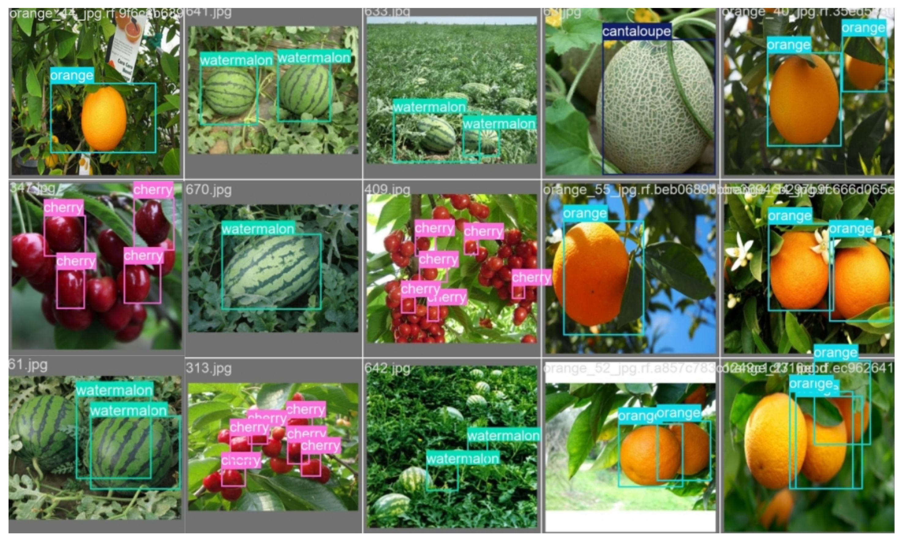
3.2.3. Generalization Assessment
3.2.4. Ablation Studies
3.2.5. Computational Efficiency
3.3. Limitation and Future Work
4. Conclusions
Author Contributions
Funding
Institutional Review Board Statement
Data Availability Statement
Acknowledgments
Conflicts of Interest
Appendix A. The JSON Output Format
Appendix B. Language Model JSON Specification
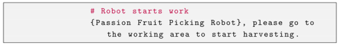
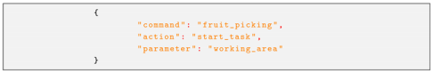
Appendix B.1. Start Harvesting Task
Appendix B.2. End Harvesting Task


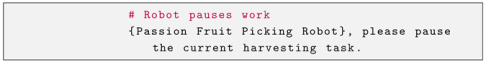
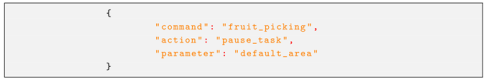
Appendix B.3. Pause Work
Appendix B.4. Resume Work


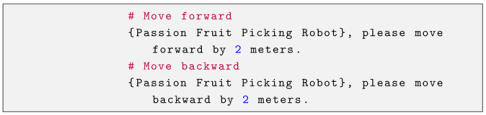
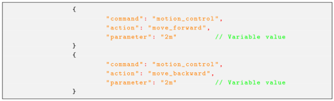
Appendix B.5. Robot Voice-Controlled Movement
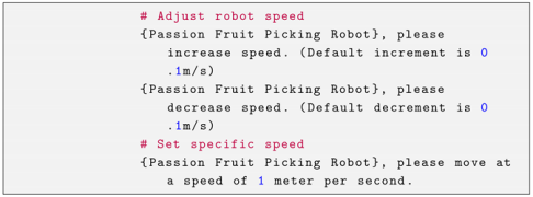
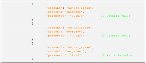
Appendix B.6. Speed Adjustment Control
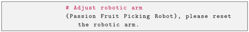
Appendix B.7. Reset Arm Position

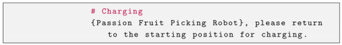
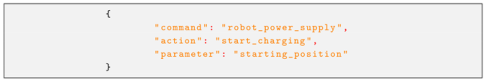
Appendix B.8. Self-Charging
Appendix C. Command Extraction and Entity Recognition Results

| ID | Original Command | Action | Entity |
|---|---|---|---|
| 1 | For semi-ripe apples, use special tools for picking. | Picking | Semi-ripe apples |
| 2 | Start from the edge of the orchard and gradually move inward to pick ripe apples. | Picking | Ripe apples |
| 3 | After rain, check and pick brighter apples. | Checking, Picking | Brighter apples |
| 4 | Use sensors to detect sugar content and decide when to pick unripe apples. | Deciding Picking Time | Unripe apples |
| 5 | Pick those that are close to full ripeness but have not yet fallen. | Picking | Nearly fully ripe apples |
| 6 | To ensure quality, prioritize picking apples with smooth and undamaged surfaces. | Prioritize Picking | Smooth and undamaged apples |
| 7 | Create a picking route mAP@[0.5:0.95] in the orchard to plan the picking of different types of apples. | Planning Picking | Different types of apples |
| 8 | Use drones to assist in locating hard-to-reach apples. | Assisting Location | Apples |
| 9 | Utilize AI vision systems to analyze the optimal picking time for apples. | Analyzing Picking | Apples |
| 10 | Record the location of each apple during picking for subsequent management. | Recording Location | Apples |
| 11 | To protect the environment, pick wild apples without disrupting the ecosystem. | Picking | Wild apples |
| 12 | By comparing the characteristics of different varieties, learn how to more Accuracyurately pick apples. | Learning Picking | Apples |
| 13 | Combine weather forecast information to schedule picking activities ahead of time to ensure the quality of apples. | Scheduling Picking | Apples |
| 14 | Improve picking techniques using machine learning to increase efficiency while reducing damage to apples. | Improving Picking Techniques | Techniques |
| 15 | At night, use infrared cameras to help pick apples that ripen at night. | Helping Picking | Nightly ripe apples |
| 16 | Develop specialized applications to guide workers on correctly picking various types of apples. | Guiding Picking | Various types of apples |
| 17 | Train pickers to understand the best picking methods for each type of apple. | Training Picking | Picking methods |
| 18 | For special events, carefully select and pick the highest quality apples. | Carefully Selecting, Picking | Highest quality apples |
| 19 | Through community cooperation, jointly participate in the local orchard’s apple picking work. | Participating Picking | Apples |
| 20 | During the harvest season, organize volunteersto pick large quantities of ripe apples together. | Organizing Picking | Ripe apples |
| 21 | Pick wild apples from bushes near the ground. | Picking | Wild apples |
| 22 | Find the highest branches and pick the largest apples there. | Picking | Largest apples |
| 23 | When detecting specific colors, pick high-hanging apples. | Picking | Specific color apples |
| 24 | On dewy mornings, pick fresh apples before the dew dries. | Picking | Fresh apples |
| 25 | Carefully distinguish and only pick fully ripe apples. | Picking | Fully ripe apples |
| 26 | Avoid damaging surrounding leaves and precisely pick the hard apples. | Precisely Picking | Hard apples |
| 27 | Find and pick hidden apples among dense foliage. | Picking | Hidden apples |
| 28 | Use image recognition technology to assist in picking rare apples. | Assisting Picking | Rare apples |
| 29 | Adjust strategies Accuracyording to seasonal changes to pick suitable apples. | Adjusting Picking | Apples |
| 30 | Optimize routes efficiently to pick multiple apples using smart algorithms. | Optimizing Path, Picking | Apples |
| 31 | Carefully pick ripe apples from fruit trees. | Carefully Picking | Ripe apples |
| 32 | Instruct robots to go to the orchard to select and pick fresh apples. | Selecting, Picking | Fresh apples |
| 33 | Use robotic arms to Accuracyurately pick brightly colored apples. | Accuracyurately Picking | Brightly colored apples |
| 34 | In greenhouses, search for and pick ripe clusters of apples. | Searching, Picking | Ripe clusters of apples |
| 35 | Detect and pick small apples hanging on lower branches. | Detecting, Picking | Small apples |
| 36 | Identify and pick apples whose color has changed from green to red. | Identifying, Picking | Green to red apples |
| 37 | Confirm the fruit is ripe and then start picking round apples. | Confirming, Picking | Round apples |
| 38 | Select and pick apples based on size and color. | Selecting, Picking | Apples |
| 39 | Remove apples that have changed color from the tree. | Removing | Changed color apples |
| 40 | Safely pick soft apples from vines or branches. | Safely Picking | Soft apples |
| 41 | Use drones to take aerial photos to help locate apples that need picking. | Helping Locating | Apples |
| 42 | Robots selectively pick apples based on preset maturity criteria. | Selectively Picking | Apples |
| 43 | Set up an automatic navigation system in the orchard to assist in picking apples. | Assisting Picking | Apples |
| 44 | Develop new picking algorithms to adapt to different sizes and shapes of apples. | Developing Algorithms | Apples |
| 45 | Apply augmented reality (AR) technology to guide pickers to find the best locations for apples. | Guiding Picking | Apples |
| 46 | Conduct a comprehensive scan of all apples in a specific area before starting to pick. | Scanning, Picking | Apples |
| 47 | Use laser rangefinders to determine the exact position of each apple. | Determining Position | Apples |
| 48 | Integrate environmental sensors to monitor weather conditions, optimizing the timing for picking unripe apples. | Monitoring, Optimizing | Unripe apples |
| 49 | Employ wearable devices like smart glasses to assist workers in efficient picking of apples. | Assisting Picking | Apples |
| 50 | Use machine vision recognition technology to Accuracyurately locate apples against complex backgrounds. | Locating | Apples |
| 51 | Determine the optimal picking time by detecting color changes in fruits to start picking apples. | Detecting, Picking | Apples |
| 52 | Instruct robots to search and only pick apples that meet specific maturity standards. | Searching, Picking | Maturity standard apples |
| 53 | Assess the hardness of the fruit with sensors to determine the picking time, ensuring apples are at their best maturity. | Assessing, Picking | Apples |
| 54 | When detected sugar content reaches peak, instruct robots to pick ripe apples. | Instructing, Picking | Ripe apples |
| 55 | Use image recognition technology to analyze surface features of the fruit, selecting high-maturity apples. | Analyzing, Picking | High-maturity apples |
| 56 | Identify and prioritize picking fully ripe apples. | Identifying, Prioritizing Picking | Fully ripe apples |
| 57 | Screen and pick apples that meet predefined maturity parameters. | Screening, Picking | Apples |
| 58 | Confirm that the size and color of the fruit meet maturity requirements before initiating the picking program for apples. | Confirming, Initiating | Apples |
| 59 | Predict the optimal maturity of each type of apple using machine learning algorithms to schedule picking times. | Predicting, Scheduling | Apples |
| 60 | Regularly monitor environmental conditions (such as temperature, humidity) to optimize the picking plan and ensure the maturity of apples. | Monitoring, Optimizing | Apples |
| 61 | Based on fruit growth cycle data, intelligently determine when to pick apples. | Determining, Picking | Apples |
| 62 | Perform a quick check before picking to ensure all selected apples have reached the expected maturity. | Checking, Ensuring | Apples |
| 63 | Use infrared imaging technology to assist in judging the internal maturity of apples, guiding precise picking. | Judging, Guiding | Apples |
| 64 | Combine weather forecast information to plan picking activities in advance, ensuring apples are picked at optimal maturity. | Planning, Ensuring | Apples |
| 65 | Use automated systems to monitor the development progress of each apple, determining specific picking dates. | Monitoring, Determining | Apples |
| 66 | Dynamically adjust picking strategies during the process to Accuracyommodate different types of apples based on real-time maturity analysis. | Analyzing, Adjusting | Apples |
| 67 | Develop dedicated software to help growers identify which apples have reached ideal maturity, ready for picking. | Developing Software, Helping | Apples |
| 68 | Collect data through wireless sensor networks, analyzing and predicting the maturity trends of apples on each tree. | Collecting, Analyzing, Predicting | Apples |
| 69 | Use AI models to simulate the maturation process of apples under different environmental conditions, providing scientific picking suggestions. | Simulating, Providing | Apples |
| 70 | Equip multi-spectral cameras for precise assessment of apple maturity, executing picking tasks Accuracyordingly. | Assessing, Executing | Apples |
| 71 | Differentiate between semi-ripe and fully ripe apples, selecting appropriate picking targets as needed. | Differentiating, Selecting | Apples |
| 72 | Accuracyurately predict the maturity of apples by referencing historical data and current environmental conditions, scheduling picking Accuracyordingly. | Predicting, Scheduling | Apples |
| 73 | Use machine vision systems to perform 3D scans of fruits to assess their shape and maturity, deciding whether to pick apples. | Scanning, Assessing, Deciding | Apples |
| 74 | Leverage deep-learning-based algorithms enabling robots to efficiently recognize and pick mature apples in complex backgrounds. | Recognizing, Picking | Apples |
| 75 | Before picking, conduct gentle touch tests to verify if apples are sufficiently ripe. | Testing, Verifying | Apples |
| 76 | Set multiple maturity thresholds to allow robots to flexibly handle the picking needs of different types of apples. | Setting, Handling | Apples |
| 77 | Judge maturity based on the aroma release pattern of the fruit, selectively picking suitable apples. | Judging, Picking | Apples |
| 78 | Continuously update information about the maturity of apples during the picking process, enhancing picking efficiency and quality. | Updating, Enhancing | Apples |
| 79 | Combine various non-invasive detection methods, such as sound waves and spectral analysis, to determine the maturity of apples. | Combining, Determining | Apples |
| 80 | Robots remotely control picking actions based on cloud platform data analysis capabilities, ensuring only correctly matured apples are picked. | Controlling, Ensuring | Apples |
| 81 | Receive real-time feedback through mobile applications, adjusting the robot’s maturity evaluation standards for apples. | Receiving, Adjusting | Apples |
| 82 | Recognize prematurely or delayed-ripening apples due to weather reasons, adjusting picking strategies Accuracyordingly. | Recognizing, Adjusting | Apples |
| 83 | Customize maturity detection schemes based on the characteristics of different varieties of apples, improving picking Accuracy. | Customizing, Improving | Apples |
| 84 | Utilize blockchain to record the entire process from sowing to picking, ensuring transparency and traceability of maturity information for each apple. | Recording, Ensuring | Apples |
| 85 | Flexibly adjust picking operations for apples based on user-set maturity preferences. | Adjusting | Apples |
| 86 | Before picking, confirm the final maturity of apples, avoiding premature or late picking. | Confirming, Avoiding | Apples |
| 87 | Simulate natural pollination processes to promote fruit development, ensuring apples reach ideal maturity at picking time. | Promoting, Ensuring | Apples |
| 88 | Use virtual reality (VR) training modules to familiarize operators with how to judge the maturity of different kinds of apples. | Training, Judging | Apples |
| 89 | Instantly evaluate and select the ripest apples during the picking process. | Evaluating, Selecting | Apples |
| 90 | See those very bright-colored apples? It’s time to pick them. | Picking | Bright-colored apples |
| 91 | This morning I noticed some apples started changing color; please help me pick these ripe fruits. | Picking | Ripe fruits |
| 92 | Can you gently pick those just perfectly ripe apples in the orchard while the dew is still on? | Picking | Perfectly ripe apples |
| 93 | When you lightly touch those hanging apples on the tree, if they feel soft but not mushy, please pick them. | Picking | Soft but not mushy apples |
| 94 | Look at those darker-colored apples at the top of the tree; please help me pick them. | Picking | Darker-colored apples |
| 95 | Accuracyording to the weather forecast, these days are perfect for picking; please prepare in advance and do not miss any batch of ripe apples. | Preparing, Picking | Ripe apples |
| 96 | The greenhouse environment is well controlled; robot, you can check and pick those apples that have ripened ideally. | Checking, Picking | Ripe apples |
| 97 | Before picking, observe the color and size of each apple; choose only the perfect ones. | Observing, Choosing | Perfect apples |
| 98 | Through touch and visual inspection, determine which apples have reached ideal maturity, then carefully pick them. | Determining, Picking | Apples |
| 99 | As soon as you smell the sweet aroma in the air, it’s time to go pick those enticingly scented apples. | Picking | Enticingly scented apples |
| 100 | Monitor the weather conditions and select sunny days for picking to ensure the sweetness and quality of the apples. | Picking | apples |
References
- Chen, Z.; Lei, X.; Yuan, Q.; Qi, Y.; Ma, Z.; Qian, S.; Lyu, X. Key Technologies for Autonomous Fruit- and Vegetable-Picking Robots: A Review. Agronomy 2024, 14, 2233. [Google Scholar] [CrossRef]
- Nyyssönen, A. Vision-Language Models in Industrial Robotics. Bachelor’s Thesis, Faculty of Engineering and Natural Sciences, Tampere University, Tampere, Finland, 2024. [Google Scholar]
- Sapkota, R.; Ahmed, D.; Karkee, M. Comparing YOLOv8 and Mask R-CNN for instance segmentation in complex orchard environments. Artif. Intell. Agric. 2024, 13, 84–99. [Google Scholar] [CrossRef]
- Jiang, L.; Jiang, H.; Jing, X.; Dang, H.; Li, R.; Chen, J.; Majeed, Y.; Sahni, R.; Fu, L. UAV-based field watermelon detection and counting using YOLOv8s with image panorama stitching and overlap partitioning. Artif. Intell. Agric. 2024, 13, 117–127. [Google Scholar] [CrossRef]
- Zhou, J.; Zhang, Y.; Wang, J. A Dragon Fruit Picking Detection Method Based on YOLOv7 and PSP-Ellipse. Sensors 2023, 23, 3803. [Google Scholar] [CrossRef] [PubMed]
- Liu, W.; Anguelov, D.; Erhan, D.; Szegedy, C.; Reed, S.; Fu, C.Y.; Berg, A.C. SSD: Single Shot MultiBox Detector. In Computer Vision—ECCV 2016; Springer: Berlin/Heidelberg, Germany, 2016; pp. 21–37. [Google Scholar] [CrossRef]
- Liang, Q.; Zhu, W.; Long, J.; Wang, Y.; Sun, W.; Wu, W. A Real-Time Detection Framework for On-Tree Mango Based on SSD Network. In Proceedings of the Intelligent Robotics and Applications, Newcastle, NSW, Australia, 9–11 August 2018; Chen, Z., Mendes, A., Yan, Y., Chen, S., Eds.; Springer: Berlin/Heidelberg, Germany, 2018; pp. 423–436. [Google Scholar]
- Vasconez, J.; Delpiano, J.; Vougioukas, S.; Auat Cheein, F. Comparison of convolutional neural networks in fruit detection and counting: A comprehensive evaluation. Comput. Electron. Agric. 2020, 173, 105348. [Google Scholar] [CrossRef]
- Wang, P.; Niu, T.; He, D. Tomato Young Fruits Detection Method under Near Color Background Based on Improved Faster R-CNN with Attention Mechanism. Agriculture 2021, 11, 1059. [Google Scholar] [CrossRef]
- Xu, P.; Fang, N.; Liu, N.; Lin, F.; Yang, S.; Ning, J. Visual recognition of cherry tomatoes in plant factory based on improved deep instance segmentation. Comput. Electron. Agric. 2022, 197, 106991. [Google Scholar] [CrossRef]
- Bordes, F.; Pang, R.Y.; Ajay, A.; Li, A.C.; Bardes, A.; Petryk, S.; Mañas, O.; Lin, Z.; Mahmoud, A.; Jayaraman, B.; et al. An Introduction to Vision-Language Modeling. arXiv 2024, arXiv:2405.17247. [Google Scholar]
- Radford, A.; Kim, J.W.; Hallacy, C.; Ramesh, A.; Goh, G.; Agarwal, S.; Sastry, G.; Askell, A.; Mishkin, P.; Clark, J.; et al. Learning. arXiv 2021, arXiv:2103.00020. [Google Scholar]
- Li, J.; Li, D.; Xiong, C.; Hoi, S. BLIP: Bootstrapping Language-Image Pre-training for Unified Vision-Language Understanding and Generation. arXiv 2022, arXiv:2201.12086. [Google Scholar]
- Li, J.; Li, D.; Savarese, S.; Hoi, S. BLIP-2: Bootstrapping Language-Image Pre-training with Frozen Image Encoders and Large Language Models. arXiv 2023, arXiv:2301.12597. [Google Scholar]
- Liu, H.; Li, C.; Wu, Q.; Lee, Y.J. Visual Instruction Tuning. arXiv 2023, arXiv:2304.08485. [Google Scholar]
- Bai, J.; Bai, S.; Yang, S.; Wang, S.; Tan, S.; Wang, P.; Lin, J.; Zhou, C.; Zhou, J. Qwen-VL: A Versatile Vision-Language Model for Understanding, Localization, Text Reading, and Beyond. arXiv 2023, arXiv:2308.12966. [Google Scholar]
- Cao, Y.; Chen, L.; Yuan, Y.; Sun, G. Cucumber disease recognition with small samples using image-text-label-based multi-modal language model. Comput. Electron. Agric. 2023, 211, 107993. [Google Scholar] [CrossRef]
- Zhou, Y.; Yan, H.; Ding, K.; Cai, T.; Zhang, Y. Few-Shot Image Classification of Crop Diseases Based on Vision–Language Models. Sensors 2024, 24, 6109. [Google Scholar] [CrossRef]
- Tan, C.; Cao, Q.; Li, Y.; Zhang, J.; Yang, X.; Zhao, H.; Wu, Z.; Liu, Z.; Yang, H.; Wu, N.; et al. On the Promises and Challenges of Multimodal Foundation Models for Geographical, Environmental, Agricultural, and Urban Planning Applications. arXiv 2023, arXiv:2312.17016. [Google Scholar]
- Qing, J.; Deng, X.; Lan, Y.; Li, Z. GPT-aided diagnosis on agricultural image based on a new light YOLOPC. Comput. Electron. Agric. 2023, 213, 108168. [Google Scholar] [CrossRef]
- Jocher, G.; Qiu, J.; Chaurasia, A. Ultralytics YOLO (Version 8.0.0). 2023. Available online: https://github.com/ultralytics/ultralytics (accessed on 9 April 2025).
- Dosovitskiy, A.; Beyer, L.; Kolesnikov, A.; Weissenborn, D.; Zhai, X.; Unterthiner, T.; Dehghani, M.; Minderer, M.; Heigold, G.; Gelly, S.; et al. An Image is Worth 16x16 Words: Transformers for Image Recognition at Scale. arXiv 2021, arXiv:2010.11929. [Google Scholar]
- Vaswani, A.; Shazeer, N.; Parmar, N.; Uszkoreit, J.; Jones, L.; Gomez, A.N.; Kaiser, L.; Polosukhin, I. Attention Is All You Need. arXiv 2023, arXiv:1706.03762. [Google Scholar]
- Li, Y.; Bubeck, S.; Eldan, R.; Giorno, A.D.; Gunasekar, S.; Lee, Y.T. Textbooks Are All You Need II: Phi-1.5 technical report. arXiv 2023, arXiv:2309.05463. [Google Scholar]
- Yang, A.; Yang, B.; Hui, B.; Zheng, B.; Yu, B.; Zhou, C.; Li, C.; Li, C.; Liu, D.; Huang, F.; et al. Qwen-2 Technical Report. arXiv 2024, arXiv:2407.10671. [Google Scholar]
- Zhou, B.; Hu, Y.; Weng, X.; Jia, J.; Luo, J.; Liu, X.; Wu, J.; Huang, L. TinyLLaVA: A Framework of Small-scale Large Multimodal Models. arXiv 2024, arXiv:2402.14289. [Google Scholar]
- OpenAI. GPT-4 Technical Report. arXiv 2024, arXiv:2303.08774. [Google Scholar]
- DeepSeek-AI. DeepSeek-R1: Incentivizing Reasoning Capability in LLMs via Reinforcement Learning. arXiv 2025, arXiv:2501.12948. [Google Scholar]
- DeepSeek-AI. DeepSeek-V2: A Strong, Economical, and Efficient Mixture-of-Experts Language Model. arXiv 2024, arXiv:2405.04434. [Google Scholar]
- DeepSeek-AI. DeepSeek-V3 Technical Report. arXiv 2025, arXiv:2412.19437. [Google Scholar]
- Li, L.H.; Zhang, P.; Zhang, H.; Yang, J.; Li, C.; Zhong, Y.; Wang, L.; Yuan, L.; Zhang, L.; Hwang, J.N.; et al. Grounded Language-Image Pre-training. arXiv 2022, arXiv:2112.03857. [Google Scholar]
- Li, Y.; Xie, S.; Chen, X.; Dollar, P.; He, K.; Girshick, R. Benchmarking Detection Transfer Learning with Vision Transformers. arXiv 2021, arXiv:2111.11429. [Google Scholar]
- Zhao, Y.; Lv, W.; Xu, S.; Wei, J.; Wang, G.; Dang, Q.; Liu, Y.; Chen, J. DETRs Beat YOLOs on Real-time Object Detection. arXiv 2024, arXiv:2304.08069. [Google Scholar]
- Zhong, Y.; Yang, J.; Zhang, P.; Li, C.; Codella, N.; Li, L.H.; Zhou, L.; Dai, X.; Yuan, L.; Li, Y.; et al. RegionCLIP: Region-based Language-Image Pretraining. arXiv 2021, arXiv:2112.09106. [Google Scholar]
- Zhao, X.; Chen, Y.; Xu, S.; Li, X.; Wang, X.; Li, Y.; Huang, H. An Open and Comprehensive Pipeline for Unified Object Grounding and Detection. arXiv 2024, arXiv:2401.02361. [Google Scholar]
- Khanam, R.; Hussain, M. What is YOLOv5: A deep look into the internal features of the popular object detector. arXiv 2024, arXiv:2407.20892. [Google Scholar]
- Yaseen, M. What is YOLOv8: An In-Depth Exploration of the Internal Features of the Next-Generation Object Detector. arXiv 2024, arXiv:2408.15857. [Google Scholar]
- Khanam, R.; Hussain, M. YOLOv11: An Overview of the Key Architectural Enhancements. arXiv 2024, arXiv:2410.17725. [Google Scholar]


| Category | Maturity | Total Instances | Category | Maturity | Total Instances |
|---|---|---|---|---|---|
| Apple | Mature | ||||
| Semi-mature | 568 | Lychee | - | 448 | |
| Immature | |||||
| Banana | Mature | ||||
| Semi-mature | 217 | Lemon | - | 451 | |
| Immature | |||||
| Grapes | Mature | ||||
| Semi-mature | 395 | Pear | - | 451 | |
| Immature | |||||
| Strawberry | Mature | ||||
| Semi-mature | 265 | Tomato | - | 357 | |
| Immature | |||||
| Persimmon | Mature | ||||
| Semi-mature | 379 | Mango | - | 1223 | |
| Immature | |||||
| Peach | Mature | ||||
| Semi-mature | 1308 | ||||
| Immature | |||||
| Passion Fruit | Mature | ||||
| Semi-mature | 708 | ||||
| Immature | |||||
| Total | 3840 | Total | 2930 | ||
| Total: | 6770 | ||||
| Component | Specification | Usage |
|---|---|---|
| GPU | NVIDIA RTX 4090D | Model inference and computation acceleration |
| CPU | AMD EPYC 9754 | Data preprocessing and backend services |
| Memory | 60 GB | Store model parameters, intermediate cache, and temporary data |
| Storage | System Disk: 30 GB SSD; Data Disk: 50 GB SSD | Fast loading of training data and model files |
| Component | Version | Usage |
|---|---|---|
| Operating System | Ubuntu 22.04 | Provides a reliable runtime environment |
| Framework | PyTorch 2.5.1 | Supports model training and inference |
| Python Environment | Python 3.12 | Manages script execution and dependencies |
| CUDA Toolkit | CUDA 12.4 | Enables GPU acceleration for deep learning |
| Model | Input Length (Chinese Characters) | Quantization | GPU Num | Speed (Tokens/s) | Accuracy (%) |
|---|---|---|---|---|---|
| Phi-2 [24] | 30–50 | BF16 | 1 | 42.5 | 91.00 |
| Phi-2 [24] | 30–50 | GPTQ-Int4 | 1 | 47.3 | 91.40 |
| Phi-2 [24] | 30–50 | AWQ | 1 | 43.9 | 90.7 |
| Qwen2-7B [25] | 30–50 | BF16 | 1 | 34.7 | 95.10 |
| Qwen2-7B [25] | 30–50 | GPTQ-Int4 | 1 | 36.2 | 94.80 |
| Qwen2-7B [25] | 30–50 | AWQ | 1 | 33.1 | 93.80 |
| TinyLlava [26] | 30–50 | BF16 | 1 | 30.5 | 91.10 |
| TinyLlava [26] | 30–50 | GPTQ-Int4 | 1 | 34.2 | 90.90 |
| GPT-4 [27] | 30–50 | BF16 | 1 | 30.2 | 94.60 |
| GPT-4 [27] | 30–50 | GPTQ-Int4 | 1 | 34.8 | 94.80 |
| GPT-4 [27] | 30–50 | AWQ | 1 | 33.6 | 93.80 |
| Deepseek-R1 [28] | 30–50 | BF16 | 1 | 21.8 | 93.60 |
| Deepseek-V2 [29] | 30–50 | FP8 | 1 | 32.2 | 95.20 |
| Deepseek-V3 [30] | 30–50 | 3-bit | 1 | 12.3 | 94.80 |
| Model | Precison | Recall | F1 Score | mAP@0.5 | mAP@[0.5:0.95] |
|---|---|---|---|---|---|
| GLIP [31] | 0.516 | 0.523 | 0.519 | 0.507 | 0.226 |
| ViTDet [32] | 0.539 | 0.554 | 0.546 | 0.542 | 0.366 |
| RTDERT [33] | 0.671 | 0.691 | 0.681 | 0.683 | 0.396 |
| RegionCLIP [34] | 0.081 | 0.089 | 0.085 | 0.084 | 0.036 |
| MM-Grounding-DINO [35] | 0.413 | 0.708 | 0.522 | 0.413 | 0.248 |
| YOLOv5 [36] | 0.682 | 0.706 | 0.694 | 0.721 | 0.568 |
| YOLOv8 [37] | 0.711 | 0.723 | 0.717 | 0.720 | 0.558 |
| YOLO11 [38] | 0.728 | 0.710 | 0.719 | 0.718 | 0.557 |
| E-CLIP (ours) | 0.778 | 0.728 | 0.752 | 0.791 | 0.652 |
| Model | Scenario | Precision | Recall | F1 Score | mAP@0.5 | mAP@[0.5:0.95] |
|---|---|---|---|---|---|---|
| GLIP | Slight Occ.—Normal Light | 0.527 | 0.531 | 0.529 | 0.528 | 0.241 |
| ViTDet | Slight Occ.—Normal Light | 0.541 | 0.564 | 0.552 | 0.553 | 0.372 |
| RTDETR | Slight Occ.—Normal Light | 0.689 | 0.701 | 0.695 | 0.693 | 0.405 |
| RegionCLIP | Slight Occ.—Normal Light | 0.096 | 0.103 | 0.099 | 0.091 | 0.042 |
| MM-Grounding-DINO | Slight Occ.—Normal Light | 0.468 | 0.874 | 0.610 | 0.468 | 0.289 |
| YOLOv5 | Slight Occ.—Normal Light | 0.728 | 0.703 | 0.715 | 0.736 | 0.575 |
| YOLOv8 | Slight Occ.—Normal Light | 0.724 | 0.728 | 0.726 | 0.729 | 0.561 |
| YOLO11 | Slight Occ.—Normal Light | 0.732 | 0.711 | 0.721 | 0.727 | 0.559 |
| E-CLIP (ours) | Slight Occ.—Normal Light | 0.836 | 0.829 | 0.832 | 0.832 | 0.661 |
| GLIP | Slight Occ.—Backlight | 0.472 | 0.481 | 0.476 | 0.462 | 0.205 |
| ViTDet | Slight Occ.—Backlight | 0.502 | 0.515 | 0.508 | 0.508 | 0.335 |
| RTDETR | Slight Occ.—Backlight | 0.623 | 0.643 | 0.633 | 0.635 | 0.362 |
| RegionCLIP | Slight Occ.—Backlight | 0.070 | 0.078 | 0.074 | 0.073 | 0.035 |
| MM-Grounding-DINO | Slight Occ.—Backlight | 0.352 | 0.700 | 0.468 | 0.352 | 0.201 |
| YOLOv5 | Slight Occ.—Backlight | 0.635 | 0.658 | 0.646 | 0.673 | 0.530 |
| YOLOv8 | Slight Occ.—Backlight | 0.663 | 0.675 | 0.669 | 0.672 | 0.520 |
| YOLO11 | Slight Occ.—Backlight | 0.678 | 0.662 | 0.670 | 0.670 | 0.519 |
| E-CLIP (ours) | Slight Occ.—Backlight | 0.702 | 0.689 | 0.695 | 0.693 | 0.589 |
| GLIP | Moderate Occ.—Normal Light | 0.427 | 0.437 | 0.432 | 0.418 | 0.183 |
| ViTDet | Moderate Occ.—Normal Light | 0.468 | 0.482 | 0.475 | 0.475 | 0.316 |
| RTDETR | Moderate Occ.—Normal Light | 0.581 | 0.602 | 0.591 | 0.593 | 0.340 |
| RegionCLIP | Moderate Occ.—Normal Light | 0.060 | 0.068 | 0.064 | 0.063 | 0.014 |
| MM-Grounding-DINO | Moderate Occ.—Normal Light | 0.337 | 0.790 | 0.473 | 0.335 | 0.276 |
| YOLOv5 | Moderate Occ.—Normal Light | 0.590 | 0.613 | 0.601 | 0.627 | 0.495 |
| YOLOv8 | Moderate Occ.—Normal Light | 0.615 | 0.628 | 0.621 | 0.628 | 0.487 |
| YOLO11 | Moderate Occ.—Normal Light | 0.632 | 0.617 | 0.624 | 0.626 | 0.485 |
| E-CLIP (ours) | Moderate Occ.—Normal Light | 0.634 | 0.665 | 0.649 | 0.651 | 0.581 |
| GLIP | Moderate Occ.—Backlight | 0.394 | 0.403 | 0.398 | 0.384 | 0.165 |
| ViTDet | Moderate Occ.—Backlight | 0.433 | 0.447 | 0.440 | 0.442 | 0.295 |
| RTDETR | Moderate Occ.—Backlight | 0.541 | 0.562 | 0.551 | 0.553 | 0.313 |
| RegionCLIP | Moderate Occ.—Backlight | 0.055 | 0.062 | 0.058 | 0.057 | 0.012 |
| MM-Grounding-DINO | Moderate Occ.—Backlight | 0.586 | 0.554 | 0.569 | 0.582 | 0.209 |
| YOLOv5 | Moderate Occ.—Backlight | 0.550 | 0.573 | 0.561 | 0.585 | 0.462 |
| YOLOv8 | Moderate Occ.—Backlight | 0.575 | 0.588 | 0.581 | 0.586 | 0.455 |
| YOLO11 | Moderate Occ.—Backlight | 0.591 | 0.577 | 0.584 | 0.583 | 0.453 |
| E-CLIP (ours) | Moderate Occ.—Backlight | 0.581 | 0.643 | 0.610 | 0.619 | 0.523 |
| GLIP | Severe Occ.—Normal Light | 0.352 | 0.362 | 0.357 | 0.345 | 0.142 |
| ViTDet | Severe Occ.—Normal Light | 0.397 | 0.410 | 0.403 | 0.403 | 0.275 |
| RTDETR | Severe Occ.—Normal Light | 0.502 | 0.523 | 0.512 | 0.514 | 0.294 |
| RegionCLIP | Severe Occ.—Normal Light | 0.048 | 0.055 | 0.051 | 0.050 | 0.012 |
| MM-Grounding-DINO | Severe Occ.—Normal Light | 0.426 | 0.759 | 0.553 | 0.426 | 0.324 |
| YOLOv5 | Severe Occ.—Normal Light | 0.512 | 0.535 | 0.523 | 0.551 | 0.435 |
| YOLOv8 | Severe Occ.—Normal Light | 0.535 | 0.548 | 0.541 | 0.548 | 0.425 |
| YOLO11 | Severe Occ.—Normal Light | 0.552 | 0.539 | 0.545 | 0.545 | 0.423 |
| E-CLIP (ours) | Severe Occ.—Normal Light | 0.552 | 0.601 | 0.575 | 0.574 | 0.483 |
| GLIP | Severe Occ.—Backlight | 0.316 | 0.325 | 0.320 | 0.308 | 0.121 |
| ViTDet | Severe Occ.—Backlight | 0.358 | 0.371 | 0.364 | 0.363 | 0.251 |
| RTDETR | Severe Occ.—Backlight | 0.462 | 0.483 | 0.472 | 0.474 | 0.261 |
| RegionCLIP | Severe Occ.—Backlight | 0.032 | 0.039 | 0.035 | 0.034 | 0.001 |
| MM-Grounding-DINO | Severe Occ.—Backlight | 0.332 | 0.595 | 0.428 | 0.328 | 0.208 |
| YOLOv5 | Severe Occ.—Backlight | 0.472 | 0.495 | 0.483 | 0.508 | 0.402 |
| YOLOv8 | Severe Occ.—Backlight | 0.495 | 0.508 | 0.501 | 0.505 | 0.395 |
| YOLO11 | Severe Occ.—Backlight | 0.512 | 0.499 | 0.505 | 0.503 | 0.393 |
| E-CLIP (ours) | Severe Occ.—Backlight | 0.513 | 0.576 | 0.543 | 0.551 | 0.462 |
| Precison | Recall | F1 Score | mAP@0.5 | mAP@[0.5:0.95] | |
|---|---|---|---|---|---|
| 1-shot | 0.431 | 0.125 | 0.194 | 0.059 | 0.049 |
| 4-shot | 0.420 | 0.438 | 0.429 | 0.387 | 0.292 |
| 8-shot | 0.596 | 0.421 | 0.493 | 0.492 | 0.340 |
| 16-shot | 0.606 | 0.618 | 0.612 | 0.646 | 0.523 |
| Precision | Recall | F1 Score | mAP@0.5 | mAP@[0.5:0.95] | |
|---|---|---|---|---|---|
| Orange | 0.505 | 0.632 | 0.561 | 0.649 | 0.442 |
| Watermelon | 0.664 | 0.610 | 0.636 | 0.619 | 0.248 |
| Cantaloupe | 0.944 | 0.615 | 0.745 | 0.819 | 0.492 |
| Cherry | 0.356 | 0.679 | 0.467 | 0.415 | 0.129 |
| All | 0.617 | 0.634 | 0.625 | 0.626 | 0.328 |
| Image–Image Module | Text–Image Module | F1 Score | mAP@0.5 | mAP@[0.5:0.95] |
|---|---|---|---|---|
| √ | √ | 0.752 | 0.791 | 0.652 |
| √ | × | 0.695 (↓0.057) | 0.683 (↓0.108) | 0.521 (↓0.131) |
| × | √ | 0.686 (↓0.066) | 0.667 (↓0.124) | 0.513 (↓0.139) |
| Precision | Recall | F1 Score | mAP@0.5 | mAP@[0.5:0.95] | |
|---|---|---|---|---|---|
| 0.0 | 0.318 | 0.638 | 0.419 | 0.396 | 0.281 |
| 0.1 | 0.357 | 0.622 | 0.453 | 0.413 | 0.306 |
| 0.2 | 0.414 | 0.641 | 0.511 | 0.523 | 0.389 |
| 0.3 | 0.445 | 0.644 | 0.526 | 0.529 | 0.390 |
| 0.4 | 0.502 | 0.553 | 0.527 | 0.614 | 0.479 |
| 0.5 | 0.638 | 0.692 | 0.663 | 0.661 | 0.512 |
| 0.6 | 0.778 | 0.728 | 0.752 | 0.791 | 0.652 |
| 0.7 | 0.445 | 0.644 | 0.526 | 0.529 | 0.39 |
| 0.8 | 0.434 | 0.656 | 0.528 | 0.532 | 0.399 |
| 0.9 | 0.337 | 0.558 | 0.421 | 0.385 | 0.281 |
| 1.0 | 0.305 | 0.707 | 0.419 | 0.387 | 0.272 |
| GFLOPs () | Parameters () | FPS | |
|---|---|---|---|
| VitDet | 321.94 | 563.20 | 26.45 |
| RTDERT | 231.72 | 409.23 | 28.79 |
| GLIP | 415.17 | 954.19 | 18.76 |
| RegionCLIP | 518.52 | 923.01 | 14.79 |
| MM-Grounding-DINO | 39.61 | 201.26 | 4.76 |
| YOLOv5 | 24.1 | 9.13 | 135.14 |
| YOLOv8 | 28.7 | 11.15 | 272.27 |
| YOLO11 | 6.50 | 2.60 | 83.33 |
| E-CLIP (ours) | 98.61 | 86.42 | 54.82 |
Disclaimer/Publisher’s Note: The statements, opinions and data contained in all publications are solely those of the individual author(s) and contributor(s) and not of MDPI and/or the editor(s). MDPI and/or the editor(s) disclaim responsibility for any injury to people or property resulting from any ideas, methods, instructions or products referred to in the content. |
© 2025 by the authors. Licensee MDPI, Basel, Switzerland. This article is an open access article distributed under the terms and conditions of the Creative Commons Attribution (CC BY) license (https://creativecommons.org/licenses/by/4.0/).
Share and Cite
Zhang, Y.; Shao, Y.; Tang, C.; Liu, Z.; Li, Z.; Zhai, R.; Peng, H.; Song, P. E-CLIP: An Enhanced CLIP-Based Visual Language Model for Fruit Detection and Recognition. Agriculture 2025, 15, 1173. https://doi.org/10.3390/agriculture15111173
Zhang Y, Shao Y, Tang C, Liu Z, Li Z, Zhai R, Peng H, Song P. E-CLIP: An Enhanced CLIP-Based Visual Language Model for Fruit Detection and Recognition. Agriculture. 2025; 15(11):1173. https://doi.org/10.3390/agriculture15111173
Chicago/Turabian StyleZhang, Yi, Yang Shao, Chen Tang, Zhenqing Liu, Zhengda Li, Ruifang Zhai, Hui Peng, and Peng Song. 2025. "E-CLIP: An Enhanced CLIP-Based Visual Language Model for Fruit Detection and Recognition" Agriculture 15, no. 11: 1173. https://doi.org/10.3390/agriculture15111173
APA StyleZhang, Y., Shao, Y., Tang, C., Liu, Z., Li, Z., Zhai, R., Peng, H., & Song, P. (2025). E-CLIP: An Enhanced CLIP-Based Visual Language Model for Fruit Detection and Recognition. Agriculture, 15(11), 1173. https://doi.org/10.3390/agriculture15111173