Hybrid Deep Learning Approaches for Improved Genomic Prediction in Crop Breeding

Abstract

Genomic selection plays a crucial role in breeding programs designed to improve quantitative traits, particularly considering the limitations of traditional methods in terms of accuracy and efficiency. Through the integration of genomic data, breeders are able to obtain more accurate predictions of breeding values. In this study, we proposed and evaluated four deep learning architectures—CNN-LSTM, CNN-ResNet, LSTM-ResNet, and CNN-ResNet-LSTM—that are specifically designed for genomic prediction in crops. After conducting a comprehensive evaluation across multiple datasets, including those for wheat, corn, and rice, the LSTM-ResNet model exhibited superior performance by achieving the highest prediction accuracy in 10 out of 18 traits across four datasets. Additionally, the CNN-ResNet-LSTM model demonstrated notable results, showcasing the best predictive performance for four traits. These findings underscore the efficacy of hybrid models in identifying complex patterns, as they integrate skip connections to mitigate the vanishing gradient problem and enable the extraction of hierarchical features while elucidating intricate relationships among genetic markers. Our analysis of SNP sampling indicated that maintaining SNP counts within the range of 1000 to the full set significantly influences prediction efficiency. Furthermore, we conducted a comprehensive comparative analysis of predictive performance among random selection, marker-assisted selection, and genomic selection utilizing wheat datasets. Collectively, these results provide significant insights into crop genetics, enhancing breeding predictions and advancing global food security and sustainability.

1. Introduction

Genomic selection (GS) represents a revolutionary tool in plant breeding, significantly accelerating the development of improved crop varieties with enhanced traits through the utilization of high-density genome-wide molecular markers for predicting the breeding values across diverse traits [1]. GS empowers breeders to make selections based on detailed genomic information, thereby facilitating earlier and more precise predictions of performance. This approach substantially decreases the duration required to complete breeding cycles, thus accelerating the release of new varieties that possess desired traits [2]. Traditional breeding methods frequently depend on phenotypic selection, which can be susceptible to environmental influences and may not reliably reflect the genetic potential of individuals. Marker-Assisted Selection (MAS) is a sophisticated breeding methodology that leverages known genetic markers linked to desirable traits to enhance the precision and efficiency of selection processes. By enabling the early identification of promising candidates, MAS expedites the breeding cycle and diminishes dependence on traditional phenotype-based selection approaches. Furthermore, Genome-Wide Association Studies (GWAS) serve as a complementary technique by systematically analyzing the entire genome of multiple individuals to identify novel genetic variants associated with specific traits. While MAS directly applies pre-identified markers for immediate application in breeding programs, GWAS focuses on uncover associations across the genome, enhancing our understanding of the genetic underpinnings of complex traits. Essentially, MAS is targeted and applied, whereas GWAS is exploratory and research- focused. In contrast, GS utilizes high-density genome-wide molecular markers to predict genomic breeding value more accurately, thereby reducing the influence of environmental variability [3].

GS employs three principal methodologies: statistical models, machine learning (ML), and deep learning (DL). Each approach offers unique advantages in predicting breeding values and elucidating genetic architectures [4]. Statistical methods, such as Genomic Best Linear Unbiased Prediction (GBLUP) [5] and ridge regression Best Linear Unbiased Prediction (rrBLUP) [6], extend the traditional BLUP framework by integrating genomic data. Bayesian models, such as Ridge Regression (BRR), BayesA, BayesB, and BayesC, utilize a Gaussian prior distribution on marker effects within a Bayesian framework, thereby facilitating the estimation of breeding values [7,8]. These models effectively predict breeding values by assuming a linear relationship between marker effects and trait performance, encompassing both additive and non-additive effects [9]. They are computationally efficient and easy to implement, which has made them popular choices for GS in various crops. However, traditional statistical methods often fail to capture nonlinear effects and lack self-learning capabilities [10]. To address these limitations, ML techniques are increasingly being utilized in genomic selection. ML provides a flexible framework capable of handling complex nonlinear relationships and continuously improve predictive performance as the volume of available data increases [10]. Notable machine learning models used in genomic selection include Random Forest (RF), Support Vector Machines (SVM), Reproducing Kernel Hilbert Space (RKHS), and Kernel Additive Models (KAML) [11,12].

DL has emerged as a powerful extension of machine learning, leveraging neural networks to identify complex patterns within data [13,14]. Notable architectures in this domain, including Multilayer Perceptrons (MLPs) [15], Convolutional Neural Networks (CNNs) [16], Long Short-Term Memory networks (LSTMs) [17], and Residual Neural Networks (ResNet) [18], have propelled significant advancements. Specifically, CNNs, designed for process grid-like data such as images, have revolutionized the field of computer vision by facilitating tasks like image classification and object detection while significantly reducing the reliance on manual feature engineering. Through convolution operations that apply the same filter across various regions of the input, CNNs effectively minimize the number of model parameters and preserve spatial invariance. LSTMs, a specialized variant of Recurrent Neural Networks (RNNs), excel in capturing long-term dependencies within sequential data, rendering them indispensable for natural language processing tasks such as machine translation and text generation. ResNet [18], developed by Kaiming He and colleagues, revolutionizes deep learning by having each layer learn residual relationships, which effectively addresses the degradation problem often encountered in deeper networks. ResNet innovative design includes cross-layer connections that create shortcut pathways, allowing inputs to be combined with convolutional results and thus enhancing overall performance. Together, these advancements underscore the transformative impact of deep learning across a wide range of applications.

Recent advancements in DL have significantly enhanced predictive capabilities in the field of plant breeding. A study conducted by Montesinos-López et al. demonstrated that DL methods outperformed GBLUP in predictive accuracy for six out of nine traits evaluated in wheat and maize [19]. The DeepGS model has also demonstrated outstanding performance in plant breeding by effectively integrating phenotypic and genomic data, thereby enhancing the predictive accuracy for complex traits [20]. The DNNGP method, developed by Wang et al., utilizes principles from CNNs and has achieved notable success across various datasets [21]. Liu et al. illustrated the superiority of single and dual CNN models over ridge regression-based best linear unbiased prediction in forecasting soybean traits, such as yield, protein content, oil content, moisture content, and plant height [22]. Furthermore, Zingaretti et al. found that DL models consistently surpassed traditional linear statistical models in predicting traits with epistatic variances in allopolyploid species such as strawberry (Fragaria × ananassa) and blueberry (Cyanococcus spp.) [23]. Notably, these studies highlight the significant potential of deep learning approaches to improve predictive accuracy for complex traits in plant breeding programs.

CNNs [24] are highly effective for feature extraction from complex, high-dimensional genomic data, enabling the capture of critical local patterns. LSTMs [25] excel at modeling sequential data, adeptly capturing temporal dependencies among genes, making them suitable for genomic applications. ResNets [26] mitigate vanishing gradient issues by incorporating skip connections, facilitating deeper network training and improved feature learning. By combining these architectures into a hybrid model, we want to leverage their strengths for enhanced feature extraction and sequence modeling, which is particularly beneficial for the complexities of genomic data. As hybrid deep learning models have shown significant performance improvements in bioinformatics, this choice aligns with cutting-edge research trends and aims to enhance prediction accuracy and robustness in genomic selection [27].

In this study, we introduce hybrid algorithms combining CNN-LSTM, CNN-ResNet, LSTM-ResNet, and CNN-ResNet-LSTM for genomic selection. By leveraging genotype data from wheat, corn, and rice, we demonstrate significant improvements in prediction accuracy, particularly with the LSTM-ResNet model. Additionally, the research explores the efficiency of SNP sampling, showing that controlling SNPs between 10,000 and 15,000 enhances computational efficiency. A comparative analysis further reveals that genomic selection outperforms traditional methods, including random and marker-assisted selection, in predicting complex traits. The findings highlight the potential of these hybrid models to elevate the precision of crop trait predictions, contributing valuable insights to the field of crop genetics and promoting global food security. These models are evaluated against traditional approaches using genotype data from rice, maize, and wheat datasets to predict phenotype data. The results demonstrate a significant improvement in prediction accuracy, particularly with the LSTM-ResNet model, thereby providing a novel method to enhance the accuracy of crop trait predictions.

Currently, there is a growing body of research applying deep learning techniques to genome-wide selection. However, there is a notable lack of studies that integrate different deep learning algorithms to explore their collective effectiveness in this area. To address this gap, we employed three distinct deep learning strategies: CNN, LSTM, and ResNet in this study. By creating a hybrid model that integrates these methodologies, we aim to investigate the predictive performance of genome-wide selection. This approach of integrating various hybrid models has seen significant advancements in other fields, such as natural language processing with large language models. By leveraging the strengths of each deep learning strategy, we hope to enhance the accuracy and reliability of predictions in genome-wide selection, ultimately contributing to more efficient breeding strategies and improved trait predictions in agricultural research.

2. Materials and Methods

2.1. Datasets Used for Genomic Prediction

Four distinct datasets were utilized in this study, each representing populations of varying population sizes and species with diverse reproductive systems: wheat599, wheat2000, rice299, and G2F_2017 (as detailed in

Table 1. Datasets used in this research.

Species	Dataset	Population Size	Marker Number	Environment	Trait	Abbr.
Wheat	Wheat599	599	1279	env1	grain yield	GY
Wheat	Wheat599	599	1279	env2	grain yield	GY
Wheat	Wheat599	599	1279	env3	grain yield	GY
Wheat	Wheat599	599	1279	env4	grain yield	GY
Wheat	Wheat2000	2000	33,709	1	thousand kernel weight	TKW
Wheat	Wheat2000	2000	33,709	1	test weight	TW
Wheat	Wheat2000	2000	33,709	1	grain length	GL
Wheat	Wheat2000	2000	33,709	1	grain width	GW
Wheat	Wheat2000	2000	33,709	1	grain hardness	GH
Wheat	Wheat2000	2000	33,709	1	grain protein	GP
Rice	Rice299	299	73,147	1	filled grain percentage	FGP
Rice	Rice299	299	73,147	1	flag leaf width	FLW
Rice	Rice299	299	73,147	1	plant height	PH
Rice	Rice299	299	73,147	1	spikelet number per Panicle	SPN
Maize	G2F_2017	356	21,011	1	days to pollen	DTP
Maize	G2F_2017	356	21,011	1	ear height	EH
Maize	G2F_2017	356	21,011	1	plant height	PH
Maize	G2F_2017	356	21,011	1	yield	Y

). All data referenced in our manuscript are detailed in the references section. To aid readers in understanding the datasets, we have provided the relevant traits and SNP quantities. For those seeking a more comprehensive exploration of these datasets, we encourage referring to the cited literature.

The wheat599 dataset encompasses 599 [28] historical wheat lines sourced from the International Maize and Wheat Improvement Center (CIMMYT) Global Wheat Program (Texcoco, Mexico). This program is widely recognized for its significant contributions to enhancing wheat varieties, thereby improving productivity and resilience across diverse environments. Genotyping of these lines involved recording binary markers indicating the presence (1) or absence (0) of specific traits. Following rigorous quality control procedures, a total of 1279 DArT markers were retained for subsequent analysis.

The second dataset, designated as wheat2000, comprised 2000 Iranian bread wheat (Triticum aestivum) landraces sourced from the CIMMYT wheat gene bank (Texcoco, Mexico). These landraces were genotyped using 33,709 DArT markers [29], with each allele coded as 1 (present) or 0 (absent) for each accession, thereby providing a binary representation of the genetic variability within the dataset. The dataset includes phenotypic traits such as thousand kernel weight (TKW), test weight (TW), grain length (GL), grain width (GW), grain hardness (GH), and grain protein (GP). This allows for an in-depth analysis of the relationships between genetic markers and important agronomic characteristics.

The third dataset, referred to as the rice299 dataset, was obtained from the irrigated rice breeding program at the International Rice Research Institute (IRRI) (Los Baños, Laguna, Philippines) [30]. This dataset includes a curated collection of 73,147 single nucleotide polymorphisms (SNPs). Alongside the genetic data, phenotypic information was collected for several key traits, including filled grain percentage (FGP), flag leaf width (FLW), plant height (PH), and spikelet number per panicle (SPN).

The fourth dataset originates from the G2F project, an interdisciplinary initiative aimed at elucidating genotype-by-environment interactions in maize (United States). This project involves collaborators from multiple disciplines [31]. For the current study, 356 hybrids were selected, focusing on four key traits: Days to Pollen (DTP), Ear Height (EH), Plant Height (PH), and Yield (Y). SNPs with a minor allele frequency greater than 5% and a per-locus missing rate less than 10% were retained, resulting in a final set of 21,011 SNPs.

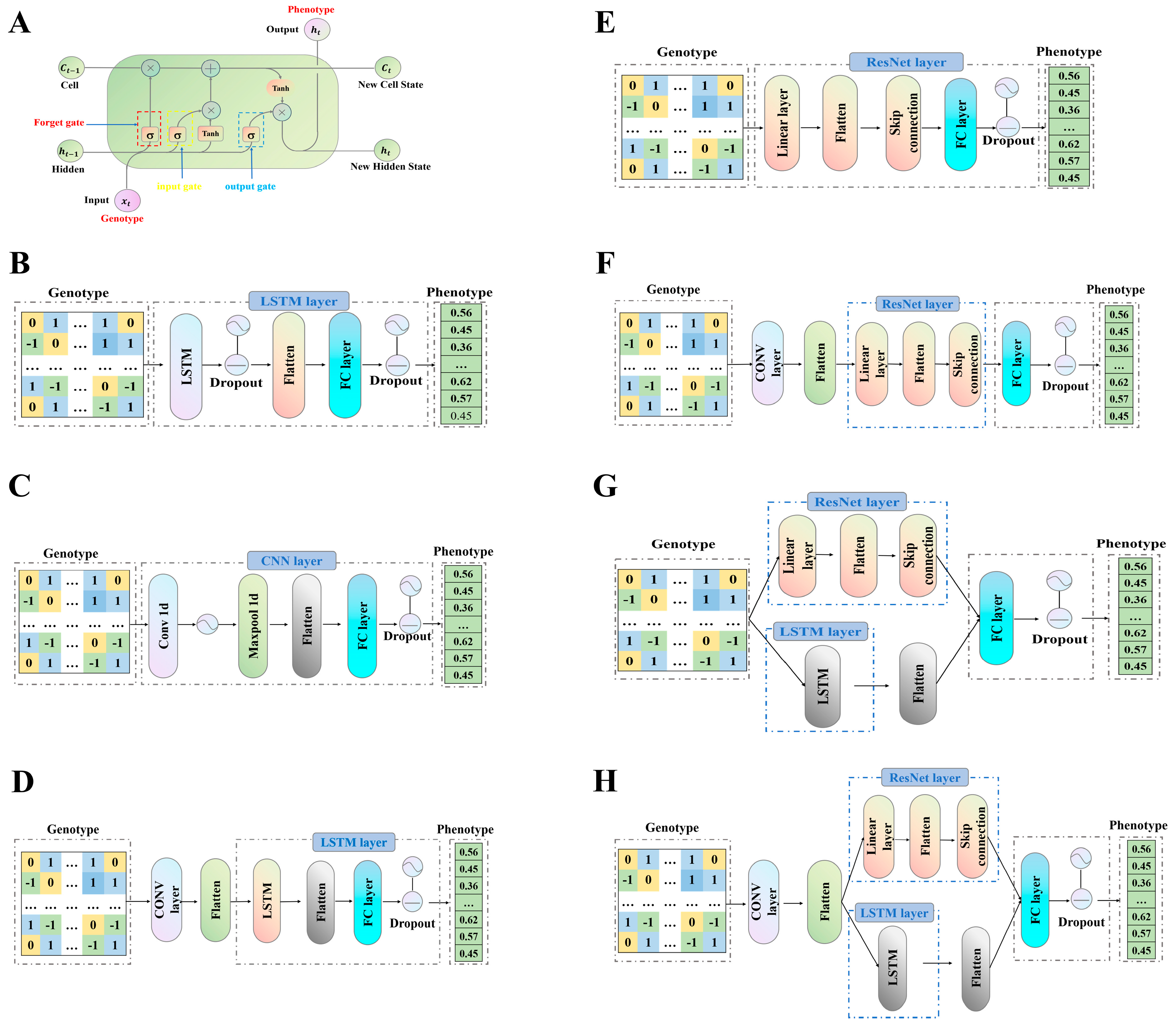
2.2. Design and Aichitecture of Hybrid Models

LSTM networks represent a specialized from of RNN that incorporates distinct components, such as the cell state, forget gate, input gate, and output gate (Figure 1A). The LSTM architecture utilized in this study includes an input layer, a forward LSTM layer, a fully connected layer, and an output layer (Figure 1B). The architecture of a CNN primarily comprises three types of layers: convolutional layers, pooling layers, and fully connected layers (Figure 1C).

To enhance the effectiveness of feature extraction and improve the model’s capability to process complex data, the CNN architecture can more accurately capture features, reduce computational complexity, and optimize information flow. This integration significantly contributes to improving the model’s performance and training efficiency (Figure 1D).

The incorporation of a ResNet architecture facilitates the convergence of deeper networks by leveraging residual learning, thereby diminishing reliance on gradients and mitigating the vanishing gradient problem. The CNN-ResNet hybrid structure integrates the depth advantages of ResNet with the feature extraction capabilities of CNNs, enabling it to manage complex tasks while preserving high training efficiency and alleviating the degradation issue that arises with network deepening (Figure 1E,F).

To address challenges such as gradient explosion and computational inefficiency associated with deep network layers, this study constructed a multi-level feature extraction module by integrating ResNets and LSTM (Figure 1G). This module aims to effectively extract features at multiple levels.

ResNet represents a significant topological structure within CNNs. CNNs consist of three essential components: convolutional layers, pooling layers, and fully connected layers. The key innovation of ResNets lies in the introduction of residual blocks, which facilitate efficient information propagation across layers and mitigate performance degradation as network depth increases.

The general formula for ResNet is presented as follows:

$$y_l=h\left(x_l\right)+F(x_l,W_l)$$

(1)

$$x_{l+1}=f\left(y_l\right)$$

(2)

Here, $x_l$ represents the input of the l layer, $F(x_l,W_l)$ denotes the convolution operation in the l layer with $W_l$ as the convolution kernel (weight matrix), $h\left(x_l\right)$ represents the identity mapping, $y_l$ represents the output of the residual block, and $f\left(y_l\right)$ denotes the activation function.

To enhance feature extraction and improve the model’s ability to process complex data, a CNN structure was integrated into the framework outlined in CNN-ResNet-LSTM. This enhancement facilitates more effective feature representation, mitigates computational complexity, and optimizes information flow, thereby significantly boosting model performance and training efficiency (Figure 1H).

2.3. Model Training Parameters

In this study, hybrid models were implemented using PyTorch 2.1 within a Python 3.11 environment on a Linux operating system [32]. PyTorch utilized GPU acceleration through CUDA 12.4 to optimize performance. We implemented a grid search method to prevent overfitting. Specifically, if the model’s predictive performance decreased in subsequent evaluations, the training process was terminated. Training parameters for the deep learning models, including the learning rate, batch size, number of epochs, and other relevant settings for each dataset, are detailed in Tables S1–S4.

Mean Squared Error (MSE) was adopted as the loss function of the hybrid models. The formula for calculating MSE is presented below.

$$MSE={\displaystyle \frac{1}{N}}{\sum }_{i=1}^n{\left(y_i-{\widehat{y}}_i\right)}^2$$

(3)

where $N$ represents the number of sample materials, $y_i$ represents a trait label, ${\widehat{y}}_i$ represents the predicted value of traits, and $y_i-{\widehat{y}}_i$ represents the residual error.

The traditional methods employed in the comparative experiments encompassed BayesA, BayesB, BayesC, and Bayesian Ridge Regression (BayesBRR). These methods were implemented using the Bayesian Generalized Linear Regression (BGLR) package [33]. The parameters settings were meticulously configured as follows: the probability that marker effects are non-zero (prob) was set to 0.5, based on the assumption that approximately half of the markers have non-zero effects. The total number of MCMC iterations (nIter) was set to 2000 to ensure sufficient model convergence and reliability. A burn-in period (burnIn) of 500 iterations was established to discard initial values and enhance model accuracy. The degrees of freedom for the prior distribution of variance (df) were set to 5, thereby providing a robust analytical framework.

2.4. Model Evaluation

We performed an extensive comparative analysis of four hybrid models—CNN-LSTM, CNN-ResNet, LSTM-ResNet, and CNN-ResNet-LSTM—against statistical models (BayesA, BayesB, BayesC, and BayesBRR), as well as standalone CNN and LSTM models. The performance of each model was assessed using 10-fold cross-validation. The dataset was randomly partitioned into 10 equal subsets (folds). A total of 10 training and testing iterations were performed. In each iteration, one subset served as the test set while the remaining nine subsets constituted the training set. Consequently, 10 evaluation outcomes were generated, and their average was taken as the final performance metric [34]. The predictive accuracy of the models was evaluated by computing the Pearson correlation coefficient (R) between the observed values and the predicted values from each model on the test set. The formula for this calculation is provided below:

$$R={\displaystyle \frac{\sum _{i=1}^n(X_i-\overline{X})(Y_i-\overline{Y})}{\sqrt{\sum _{i=1}^n{\left(X_i-\overline{X}\right)}^2}\sqrt{\sum _{i=1}^n{\left(Y_i-\overline{Y}\right)}^2}}}$$

(4)

where $n$ represents the total number of data points or samples used in the calculation, and $X_i$ denotes the individual predicted values generated by the model, while $Y_i$ refers to the individual actual values or ground truth outcomes. The mean of the predicted values is indicated by $\overline{X}$, and the mean of the actual values is represented by $\overline{Y}$.

2.5. The Impact of the Number of SNPs on Prediction Methods

We utilized the Wheat2000, Rice299, and G2F_2017 datasets to investigate the impact of SNP quantity on the model’s predictive performance. The Wheat599 dataset, comprising 1279 SNPs, was excluded from our analysis owing to its comparatively limited SNP count. This study employed a random sampling strategy to evaluate the model’s performance across different quantities of SNPs, specifically at levels of 1000, 5000, 10,000, and 15,000 SNPs. For each specified SNP quantity, 10-fold cross-validation experiments were conducted to ensure reliability and reduce potential noise. The performance was assessed using Pearson’s correlation coefficient (R).

2.6. A Comparison of the Application Effects of GS Based on LSTM-ResNet

This study employed three assisted breeding methods—Random Selection, MAS, and GS—to evaluate the efficacy of the proposed hybrid model in breeding applications. We initiated our study by conducting a GWAS [35] using the mixed linear model (MLM) [36] implemented in GAPIT 3.5 [37] software. To effectively account for population structure and genetic relatedness, we included the first two principal components from principal component analysis (PCA) [38] in our model, along with a kinship matrix. This approach allowed us to identify the top 10 and 100 SNPs with the smallest p-values as potential markers. Utilizing the effect values of these markers, we then calculated the predicted outcomes through the MAS [39] method. However, the original dataset did not provide specific chromosomal locations or physical position information for the SNPs. To simplify our analysis, we assumed that all selected SNP sites were located on the same chromosome and ordered their physical positions according to their sequence in the dataset. The detailed results of the MAS data are presented in the supplementary materials (see Supplementary Tables S6–S15).

To compare the selection efficiency of the three breeding strategies, namely GS, MAS, and random selection, we conducted a selection intensity analysis. This analytical approach quantitatively assesses the relative selection strength of various methods in improving target traits. The formula for calculating selection intensity is as follows:

$$i={\displaystyle \frac{{\overline{x}}_s-\overline{x}}{\sigma }}$$

(5)

where ${\overline{x}}_s$ denotes the mean phenotypic value of the selected individuals, $\overline{x}$ is the mean phenotypic value of the entire population, and $\sigma$ corresponds to the standard deviation of the population’s phenotypic values. The detailed procedure is illustrated in Figure 2, which outlines the steps taken in the comparison of these methods.

Step 1: Test Dataset Construction

For the Wheat599 dataset, we systematically selected a random sample of 120 instances, whereas for the Wheat2000 dataset, we randomly selected 400 instances. This initial sampling formed the foundation for our subsequent analyses, enabling us to evaluate the performance of various breeding methods on these designated subsets.

Step 2: Sampling Selection

In the second step, we implemented three methods to evaluate their effectiveness. Random Selection involved randomly choosing 50% of the samples from the test set. GS focused on selecting the top 50% of samples based on predicted phenotypes generated by the LSTM-ResNet model. MAS utilized GWAS to identify the top 10 SNPs and the 100 SNPs most strongly associated with phenotypic traits within each dataset. Subsequently, molecular markers were employed to predict phenotypes for the test set samples, and the top 50% were selected based on these predictions. By utilizing these methods, we were able to compare the proportions of the top 50% in the test set to evaluate the accuracy and efficacy of each approach.

Step 3: Validation

The final step involved evaluating the selected samples by comparing their predicted values against the observed values. For the Wheat599 dataset, we assess the selected samples relative to the top 60 samples based on observed values. Similarly, for the Wheat2000 dataset, we compared the selected samples to the top 200 samples based on observed values. This validation process enabled us to evaluate the reliability of each breeding method in accurately predicting phenotypic traits.

3. Results

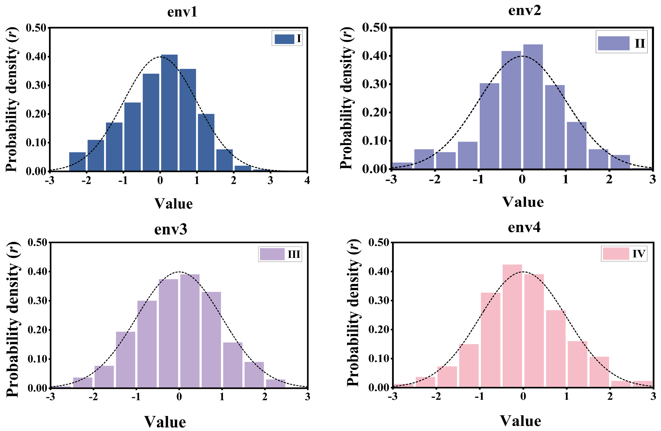
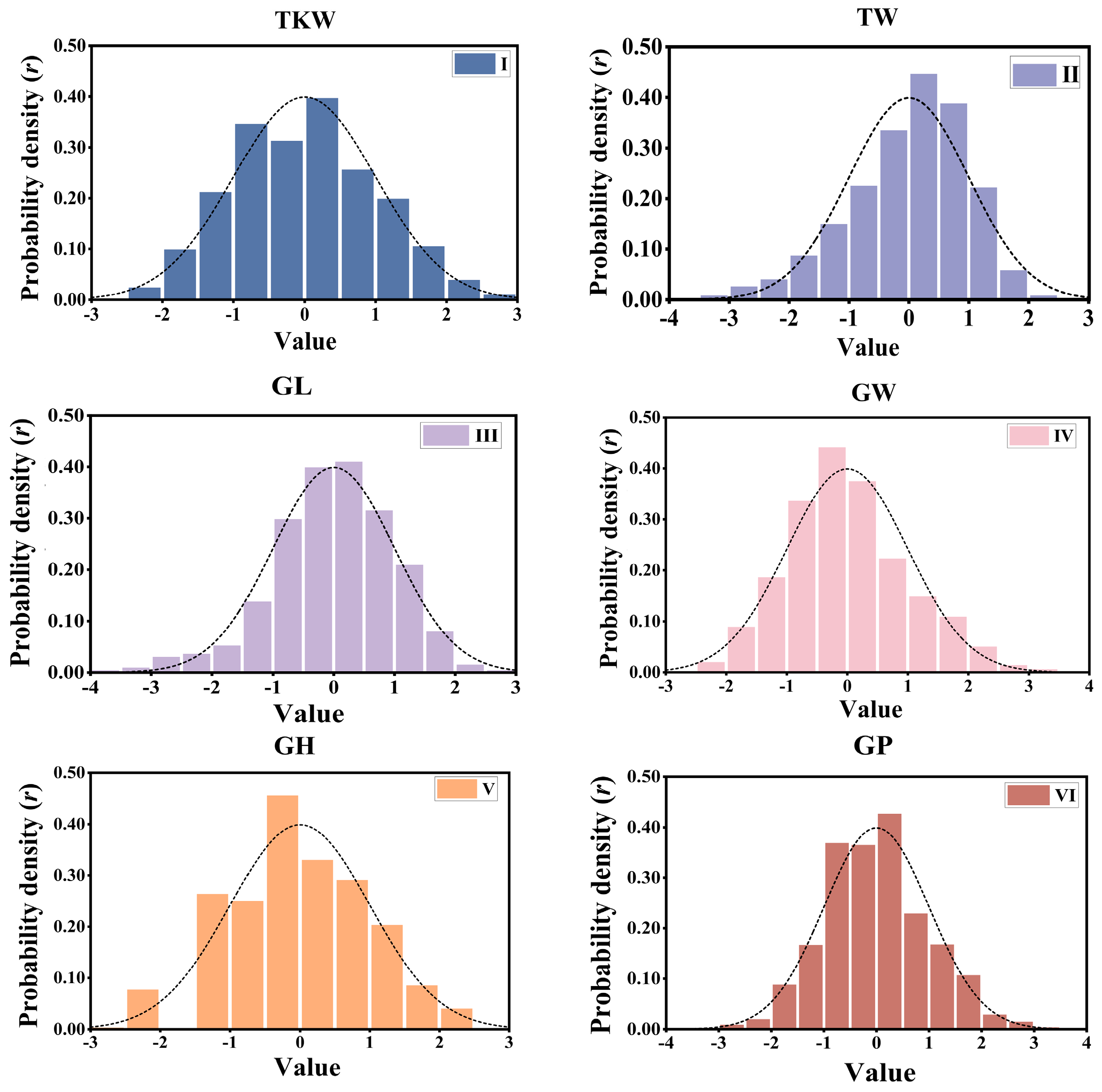
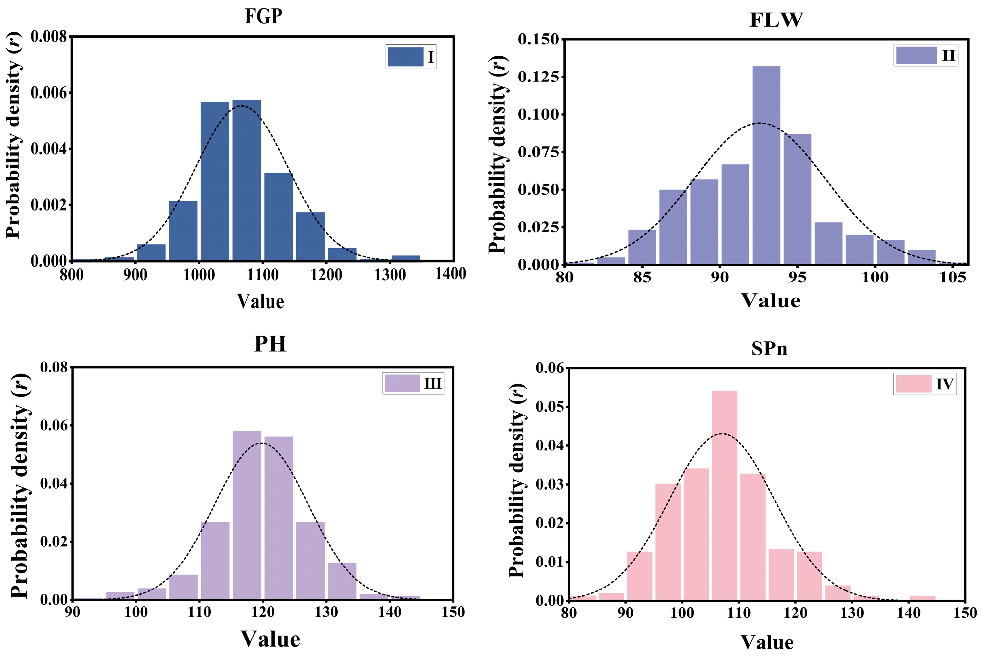
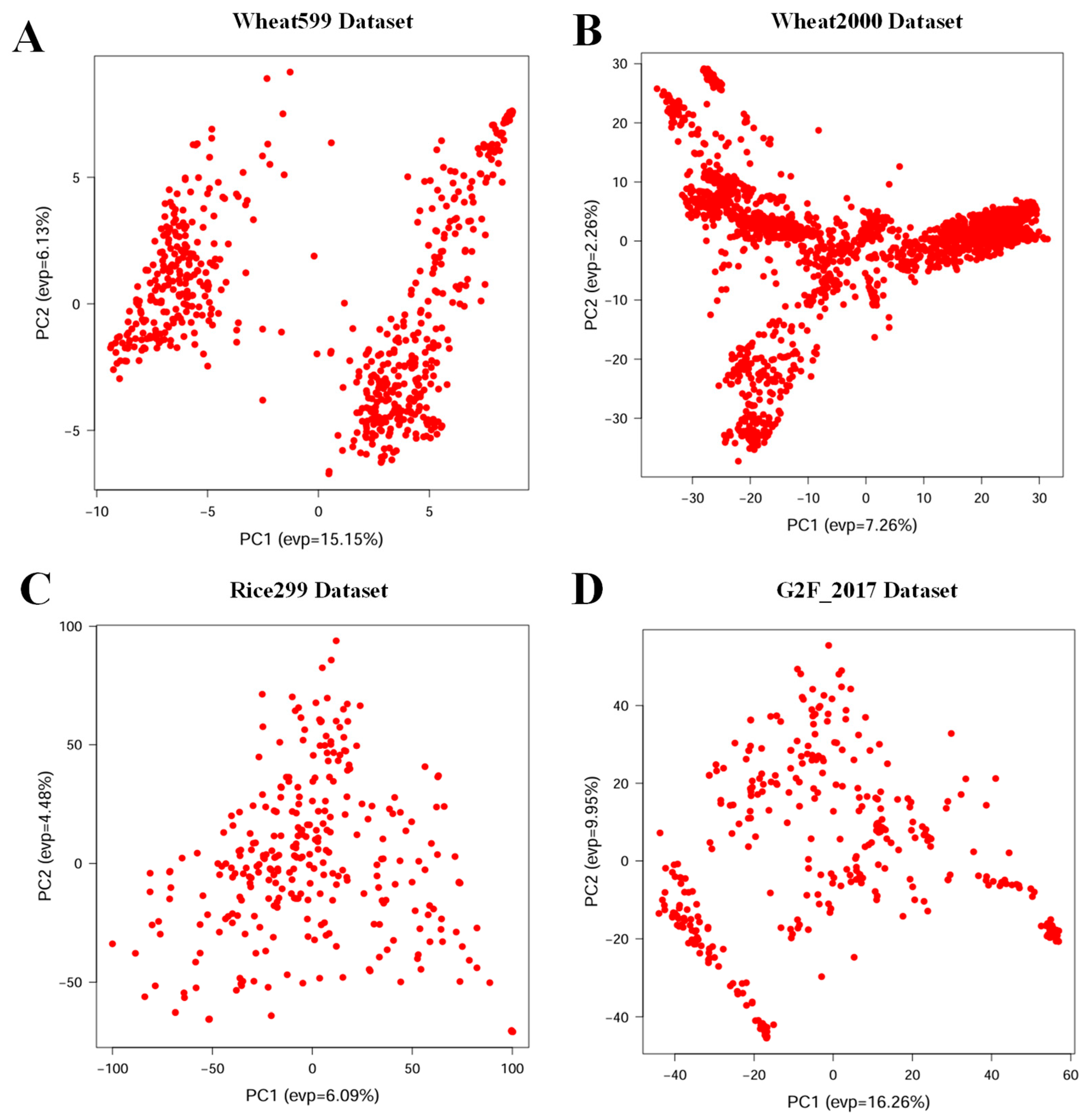
3.1. Phenotypic Distribution and Genetic Diversity

To gain a deeper understanding of the phenotypic distribution, we conducted visual analyses of the data from the datasets utilized in this study: Wheat599, Wheat2000, Rice299, and G2F. Panel A displays the frequency distributions of phenotypes from four environments within the Wheat599 dataset (Figure 3), each exhibiting similar distribution characteristics. Panel B presents six phenotypic traits from the Wheat2000 dataset (Figure 4), including Thousand Kernel Weight, Test Weight, and Grain Length, all of which showcase comparable distributions. Panel C focuses on the Rice299 dataset (Figure 5), emphasizing the variability in traits such as Percentage of Filled Grains and Plant Height. Finally, Panel D features four traits from the G2F_2017 dataset (Figure 6), highlighting the distribution patterns of Days to Pollen and Yield. Overall, the phenotypic distributions do not exhibit any unusual patterns, making them suitable for subsequent phenotypic prediction analyses.

The genetic diversity varied significantly among the four datasets. Due to the different construction methods of each crop population, the germplasm exhibited distinct distribution patterns, as indicated by a PCA that utilized SNPs from all populations as input (Figure 7). Furthermore, the rich genetic and phenotypic diversity captured in these datasets supports the validation of the accuracy and stability of the modeling algorithms employed in this study.

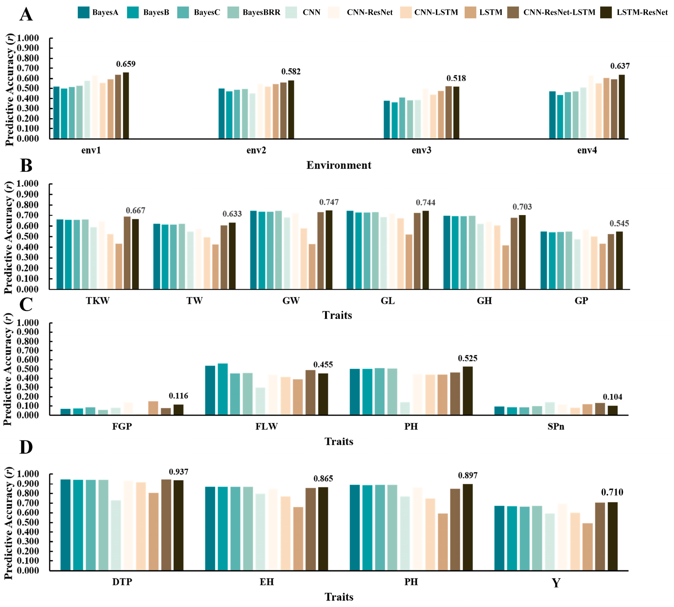
3.2. Evaluation of Prediction Accuracy for Hybrid Models and Other Methods

In this study, predictive accuracy was evaluated across four datasets (Wheat599, Wheat2000, Rice299, and G2F) by evaluating the correlation coefficients validation sets within the 10-fold cross-validation.

The predictive performances of various models on the Wheat599 validation dataset across four environments (env1, env2, env3, env4) exhibit distinct patterns in accuracy (Figure 8A, Table S5). In env1, the LSTM-ResNet model achieves the highest accuracy of 0.659, followed by CNN-ResNet at 0.632. In env2, LSTM-ResNet again leads with an accuracy of 0.582, while CNN-ResNet ranks second with 0.546. In env3, the best-performing model is CNN-ResNet-LSTM, achieving an accuracy of 0.521, closely followed by CNN-ResNet at 0.502. Finally, in env4, LSTM-ResNet leads with an accuracy of 0.637, and CNN-ResNet follows closely with 0.634. Overall, the results indicate that LSTM-ResNet consistently outperforms other models across all environments, with CNN-ResNet also demonstrating strong performance, particularly in env1 and env4.

The predictive performances of various models on the Wheat2000 validation dataset across different traits (TKW, TW, GW, GL, GH, GP) exhibit notable variations in accuracy (Figure 8B, Table S5). For TKW, CNN-ResNet-LSTM achieves the highest score of 0.687, followed closely by LSTM-ResNet at 0.667. In the TW metric, LSTM-ResNet leads with a score of 0.633, while BayesBRR follows with 0.622. For GW, LSTM-ResNet excels again with a score of 0.747, closely followed by BayesA at 0.745. In GL, both BayesA and LSTM-ResNet achieve the highest score of 0.744, with BayesBRR coming in second at 0.735. In the GH category, LSTM-ResNet once again performs best with a score of 0.703, followed closely by BayesA and BayesBRR at 0.695. Finally, for GP, CNN-ResNet achieves the highest score of 0.57, with BayesA and BayesBRR both scoring 0.545. Overall, these results underscore the superior performance of hybrid models, particularly LSTM-ResNet and CNN-ResNet-LSTM, across multiple traits in the Wheat2000 dataset.

The predictive performances of various models on the Rice299 validation dataset for different traits (FGP, FLW, PH, SPn) exhibit noticeable variations in accuracy (Figure 8C, Table S5). For FGP, the LSTM model achieves the highest score of 0.152, followed closely by CNN-ResNet with a score of 0.141. In terms of FLW, BayesB leads with a score of 0.562, while BayesA follows at 0.533. For PH, LSTM-ResNet stands out with a score of 0.525, closely trailed by BayesA at 0.502. Lastly, for the SPn trait, BayesBRR records the highest score of 0.101, followed by CNN-ResNet-LSTM at 0.135. Overall, these results highlight the varied performance of different models, with LSTM and BayesB demonstrating particularly robust performances across multiple traits in the Rice299 dataset.

The predictive performances of various models on the G2F_2017 validation dataset across different traits (DTP, EH, PH, Yield) exhibit distinct outcomes (Figure 8D, Table S5). For DTP, CNN-ResNet-LSTM achieves the highest score of 0.946, closely followed by BayesA with a score of 0.944. In terms of EH, both BayesA and BayesB achieve a score of 0.868, while CNN-ResNet follows with a score of 0.848. For PH, LSTM-ResNet excels with a score of 0.897, slightly ahead of BayesA at 0.89. Finally, in the Yield category, CNN-ResNet-LSTM leads with a score of 0.703, followed by CNN-ResNet at 0.697. Overall, the results indicate that models such as CNN-ResNet-LSTM and LSTM-ResNet demonstrate superior performance across multiple traits in the G2F_2017 dataset, consistently outperforming models like BayesA and BayesB.

3.3. Comparison of Hybrid Deep Learning Model Architectures and Their Predictive Performance

In this study, the architectures of four hybrid models—CNN-ResNet, CNN-LSTM, CNN-ResNet-LSTM, and LSTM-ResNet—were systematically structured, and the model with the highest number of top predictive performances was summarized (

Table 2. Summary of model architectures and their predictive performance.

Model/Layer	CNN Layer	Flatten Layer	ResNet Layer	Fully Connected (FC) Layer	Dropout Layer	ReLU Layer	The Quantity of Highest Scores	Traits with Highest Accuracy
CNN-ResNet	Conv1d, ReLU, Maxpool1d, Flatten	√	Linear, Flatten, Skip Connected	√	√	√	1	Wheat 2000_GP
CNN-LSTM	Conv1d, ReLU, Maxpool1d, Flatten	√	×	√	√	√	×	×
CNN-ResNet-LSTM	Conv1d, ReLU, Maxpool1d, Flatten	√	Linear, Flatten, Skip Connected	√	√	√	4	Wheat 599_env3; Wheat 2000_TKW; Rice 299_SPn; G2F_2017_DTP
LSTM-ResNet	×	×	Linear, Flatten, Skip Connected	√	√	√	10	Wheat 599_env1/env2/env4; Wheat 2000_TW/GL/GW/GH; Rice 299_PH; G2F_2017_PH/Yield
LSTM	×	×	×	√	√	√	1	Wheat 599_FGP
BayesA	×	×	×	×	×	×	1	G2F_2017_EH
BayesB	×	×	×	×	×	×	1	Rice 299_FLW

The symbol ‘√’ denotes that the model incorporates the corresponding layer, whereas ‘×’ signifies that the model excludes that particular layer.

). The comprehensive analysis of the predictive performance of 10 models across all four datasets—Wheat 599, Wheat 2000, Rice 299, and G2F 2017—revealed substantial variations in efficacy among the genomic selection models. Notably, the LSTM-ResNet model exhibited consistently superior performance across multiple traits, achieving the 10 highest prediction accuracies for 18 traits across four datasets. Notably, for key traits or environmental conditions such as Wheat599_env1/env2/env4, Wheat2000_TW/GL/GW/GH, Rice299_PH, and G2F_2017_PH/Yield, the proposed model demonstrated significantly superior predictive accuracy compared to all other models. Additionally, the CNN-ResNet-LSTM model exhibited remarkable results by achieving the highest predictive accuracy across four traits, including env3 in the Wheat 599 dataset, TKW in the Wheat 2000 dataset, SPn in the Rice 299 dataset, and DTP in the G2F 2017 dataset. Despite the overall strong performance of hybrid deep learning models, traditional models demonstrated robust competitiveness in specific contexts. For instance, BayesB achieved the highest accuracy for the FLW trait in the Rice 299 dataset, whereas BayesA showed the best performance for the EH trait in the G2F 2017 dataset (Table 2).

These results highlight the advantages of the hybrid model LSTM-ResNet in leveraging skip connections and its ability to extract hierarchical features for effectively identifying complex patterns, making it the best-performing model. This enables such models to discern intricate relationships among genetic markers. Collectively, the LSTM-ResNet and CNN-ResNet-LSTM architectures offer robust solutions for tasks requiring a comprehensive understanding of both spatial and temporal dynamics within complex datasets. Particularly, the LSTM-ResNet architecture excels in capturing complex environmental and trait patterns. Furthermore, these findings underscore the ongoing relevance of Bayesian models in specific applications.

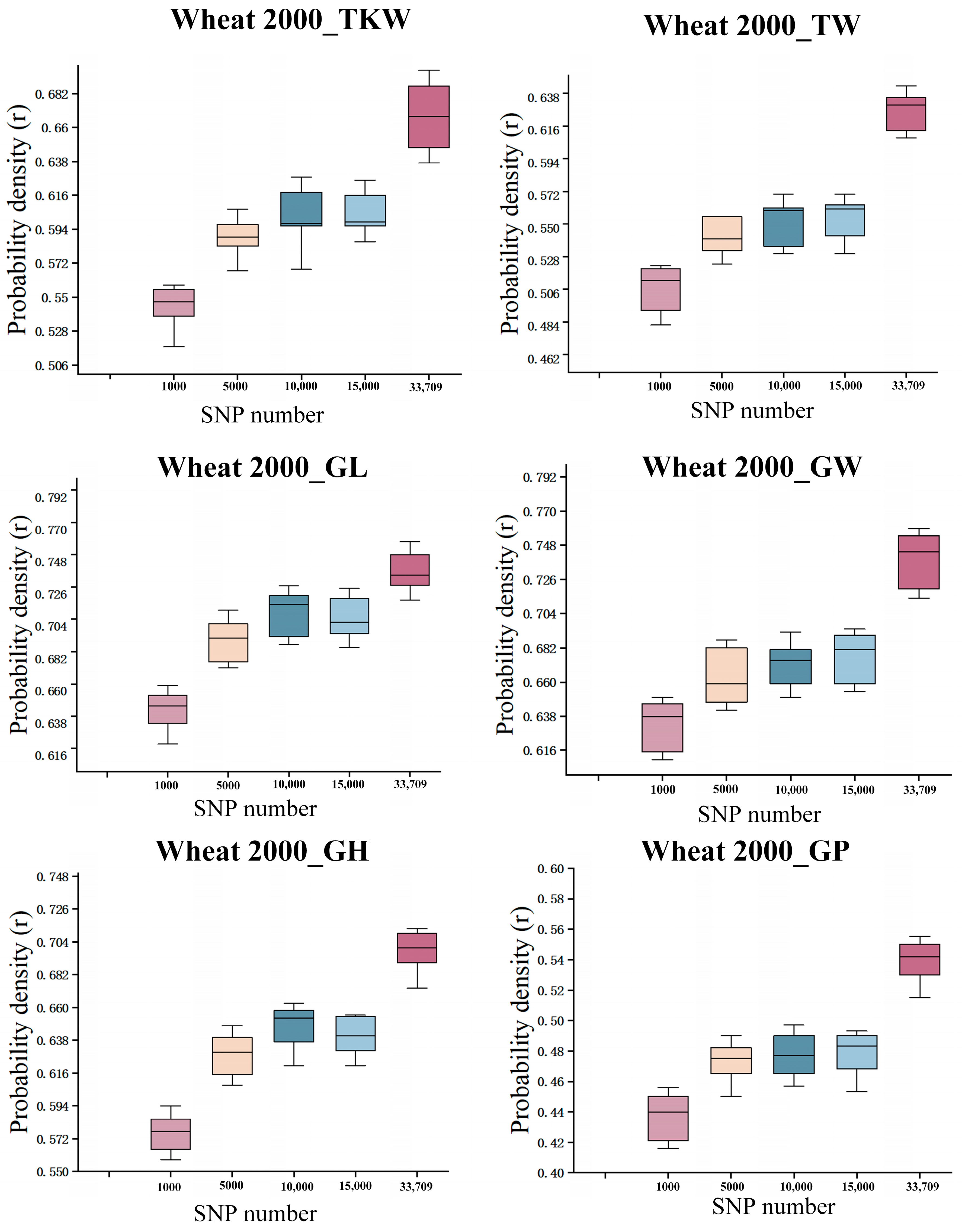
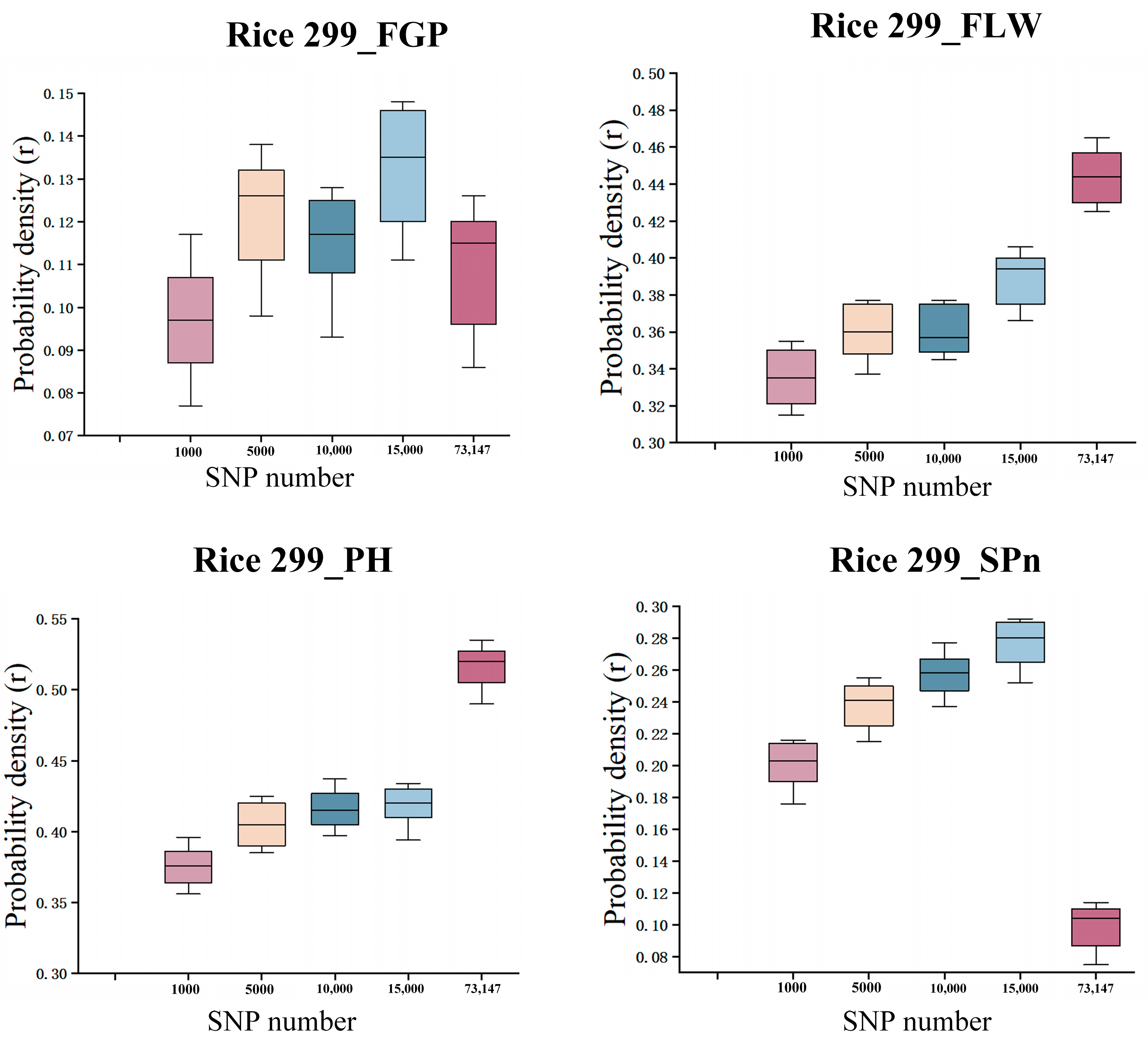
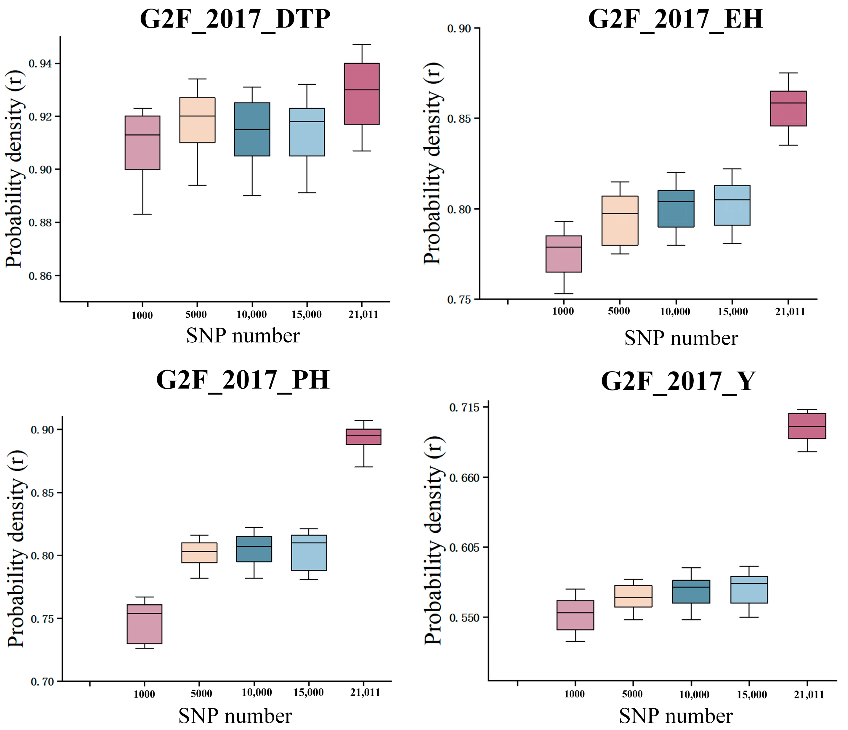
3.4. The Impact of Randomly Selecting the Number of SNPs on Prediction Methods

The number of SNPs reportedly has a significant influence on the performance of GS prediction methods [40]. The table enumerates the predictive accuracies of various traits across different datasets, namely, Wheat 2000, Rice 299, and G2F 2017, based on varying numbers of SNPs: 1000, 5000, 10,000, 15,000, and the full set of SNPs.

Using the LSTM-ResNet model on the Wheat2000 dataset, predictions were made with randomly sampled SNP subsets of different sizes (1000, 5000, 10,000, 15,000, and all 33,709 SNPs) (Figure 9). Each experiment was repeated 10 times to evaluate the model’s stability and accuracy. The six subplots in the figure correspond to six traits: thousand kernel weight (TKW), total weight (TW), grain length (GL), grain width (GW), plant height (GH), and growth period (GP). Overall, as the number of SNPs increased, the predictive performance (correlation coefficient r) generally improved, with the model performing best when using all SNPs. Additionally, the predictability varied among traits; for example, the r values for TKW, GL, and GH were generally higher than for GP, indicating stronger predictive ability of the model for certain traits. Furthermore, the improvement from 10,000 to 15,000 SNPs tended to plateau, reflecting a degree of information redundancy or diminishing marginal returns.

In the Rice299 dataset, SNP subsets of different sizes (1000; 5000; 10,000; 15,000; and all 73,147 SNPs) were randomly sampled (Figure 10), and for each subset, modeling and prediction were repeated 10 times to evaluate the prediction accuracy for four traits: FGP (filled grain percentage), FLW (flag leaf width), PH (plant height), and SPn (spikelet number). The results are shown in the figure. Overall, the predictive performance for FLW and PH steadily improved as the number of SNPs increased, reaching the highest accuracy when using all SNPs. This indicates that these two traits are more sensitive to genetic features, and that more SNP information helps the model capture their complex genetic background. For FGP and SPn, prediction performance reached a relatively high level at 15,000 SNPs but decreased when using the full set of SNPs, suggesting that excessive features may introduce redundancy or noise, which negatively impacts model performance. Model stability was assessed by repeating the sampling 10 times, and the boxplots clearly illustrate the distribution and variability of prediction results under different SNP number conditions, highlighting the importance of appropriately controlling feature dimensionality in genomic selection.

In the G2F_2017 dataset, SNP subsets of varying sizes (1000, 5000, 10,000, 15,000, and all 21,011 SNPs) were randomly selected (Figure 11), and each subset underwent 10 repeated modeling and prediction runs to assess the accuracy for four traits: days to pollen shed (DTP), ear height (EH), plant height (PH), and yield (Y). The results, shown in the figure, reveal clear trends. Prediction accuracy for EH and PH consistently improved with the increasing number of SNPs, achieving the highest performance when using the full SNP set, indicating that these traits are strongly influenced by genetic variation and benefit from comprehensive genomic information. For yield (Y), prediction accuracy improved up to 15,000 SNPs and then reached a plateau, with the full SNP set providing the best precision overall. Stability of the model predictions was confirmed through the 10-fold repeated sampling, and the boxplots effectively depict the distribution and variability of results across SNP subsets. These findings underscore the importance of balancing SNP quantity to maximize predictive power while avoiding potential noise, highlighting the critical role of feature dimension control in genomic selection.

3.5. The Application Outcomes of GS Based on LSTM-ResNet

In contemporary crop breeding, the precision and efficiency of selection methodologies are pivotal determinants of the success or failure of the breeding process [41]. With the rapid advancement of genomic technologies, random selection methods are progressively being supplanted by more advanced techniques such as GS and MAS. This study investigates the application potential of these advanced methods in crop breeding by comparing their performance relative to random selection across diverse environments and traits. In this study, MAS predictions were performed using the top 10 SNPs and 100 SNPs selected from GWAS. Detailed MAS data are available in the supplementary materials (see Supplementary Tables S6–S15).

The results presented in

Table 3. The selection intensity of GS, MAS, and Random.

Datasets	GS	MAS TOP 100 SNP	MAS TOP 10 SNP	Random
Wheat599_env1	0.539	0.569	0.281	0.021
Wheat599_env2	0.447	0.449	0.233	−0.113
Wheat599_env3	0.349	0.593	0.084	−0.168
Wheat599_env4	0.444	0.491	0.331	−0.034
Wheat2000_TKW	0.540	0.457	0.231	−0.078
Wheat2000_TW	0.463	0.104	0.097	0.022
Wheat2000_GL	0.552	0.572	0.294	−0.122
Wheat2000_GW	0.586	0.466	0.238	−0.006
Wheat2000_GH	0.591	0.538	0.235	−0.002
Wheat2000_GP	0.458	0.572	0.292	−0.052

indicate that the selection intensity of the GS model and the MAS TOP 100 model is comparable across several datasets. This suggests that utilizing the 100 SNPs most closely associated with traits can achieve prediction performance similar to that of the GS model. For instance, in multiple environments, the MAS TOP 100 scores are consistently close to those of GS, as observed in Wheat599_env1 (0.569 for MAS TOP 100 versus 0.539 for GS) and Wheat2000_GL (0.572 for MAS TOP 100 versus 0.552 for GS). However, both the GS and MAS TOP 100 models outperform the MAS TOP 10 model, which reflects weaker predictive performance due to its reliance on a smaller subset of SNPs tightly linked to the analyzed traits. For example, MAS TOP 10 exhibits significantly lower accuracies, such as 0.281 in the Wheat599_env1 dataset compared to GS and MAS TOP 100. Additionally, all three models—GS, MAS TOP 100, and MAS TOP 10—demonstrate superior performance compared to the Random model, which consistently demonstrates inferior results across all datasets. This analysis underscores the critical importance of judicious SNP selection for enhancing predictive accuracy while also highlighting that even the least effective model (MAS TOP 10) still markedly surpasses the Random model. Furthermore, these findings reinforce the conclusion that GS is better equipped to manage complex, high-dimensional genomic data, reliably identifying superior individuals.

4. Discussion

In this study, we developed four hybrid models—CNN-ResNet, CNN-LSTM, LSTM-ResNet, and CNN-ResNet-LSTM—by integrating the architectures of CNN, LSTM, and ResNet for genomic selection. To evaluate their performance, we utilized four datasets to compare the prediction accuracy of these hybrid models with that of deep learning models (CNN and LSTM) and statistical models (BayesA, BayesB, BayesC, and BayesBRR). Our findings revealed that the LSTM-ResNet model achieved the highest performance across 10 traits out of a total of 18 traits across all four datasets. Furthermore, the CNN-ResNet-LSTM model performed exceptionally well in four traits within the same datasets, while the CNN-ResNet model demonstrated superiority in one trait in the Wheat599 dataset (Table 3). These results highlight the potential value of our hybrid modeling approach. However, no single model consistently outperformed all others across every test dataset. Overall, the LSTM-ResNet hybrid model demonstrated superior performance across a wider spectrum of datasets, thereby validating its significance in the field of genomic selection predictions and suggesting avenues for the exploration of novel modeling strategies.

The use of different deep learning frameworks to build genomic prediction models has already achieved notable successes. Each of these models possesses unique characteristics that are tailored for different applications in genomic selection and agricultural data analysis. For example, DNNGP includes three CNN layers, one batch normalization layer to mitigate overfitting, and two dropout layers [21]. DeepCCR combines a convolutional neural network with bidirectional long short-term memory [42]. SoyDNGP consists of 12 convolutional layers and a single fully connected layer [43]. GPformer employs a transformer-based architecture to efficiently process time series and spatial data [44], while Cropformer integrates a CNN layer with a multi-headed self-attention mechanism [45]. These models reflect significant advancements in genomic selection and agricultural analytics, demonstrating strong competitiveness based on their distinctive methodologies. Additionally, hybrid models such as LSTM-ResNet exhibit strong performance across multiple traits, which emphasizes the necessity of continued exploration and research to enhance our understanding and application of genomic selection methodologies. However, none have consistently outperformed control methods across all traits, highlighting the considerable challenge of identifying a deep learning model with universal excellence [46]. Sustained exploration of network structures and parameter optimization remains crucial for further progress in this domain.

While the hybrid model exhibited superior performance across a broader range of traits, Bayesian methods also demonstrated impressive predictive abilities for specific traits. For instance, in predicting the EH trait of the G2F_2017 dataset, all four Bayesian methods outperformed other models. However, for other traits, Bayesian methods performed slightly less effectively than LSTM-ResNet, as observed with the GW trait in the Wheat2000 dataset (Figure 5). Indeed, Abdollahi-Arpanahi et al. noted in their comparative analysis of various genomic prediction methods that BayesB achieved higher prediction accuracy than MLP and CNN [47]. Similarly, Pook demonstrated that BayesA exhibited marginally better predictive performance compared to MLP and CNN [48]. Therefore, Bayesian methods demonstrate significant value and competitiveness compared to other approaches in specific contexts.

Furthermore, we investigated the performance of the well-performing LSTM-ResNet hybrid model with respect to feature selection. A random sampling approach was applied to all SNP markers to assess the prediction accuracy of the LSTM-ResNet model. Our findings revealed that, except for the Rice299_FGP and Rice299_SPn test datasets, the highest prediction accuracy was consistently achieved when all available SNP features were utilized. This indicates that the number of SNP features is crucial for the model’s predictive accuracy. Indeed, a similar trend was observed with LightGBM, wherein prediction accuracy increased as the number of SNP features expanded [49]. However, HGATGS did not exhibit a clear improvement in prediction accuracy with the increasing number of SNP features, which might be attributed to the hypergraph attention network architecture it employs [50]. For the Rice299_FGP and Rice299_SPn datasets, the optimal prediction accuracy was attained with 15,000 SNP features, suggesting a degree of redundancy in the features used by the LSTM-ResNet model for these particular datasets. In practical applications of genomic selection [51], it may be beneficial to reduce the number of SNP features, which could also lower the costs associated with SNP detection. Consequently, establishing an optimal number of SNPs should be aligned with the specific characteristics of the dataset in question.

In this study, we utilized a random selection approach to evaluate the impact of varying numbers of markers on prediction accuracy. However, it is important to note that multiple marker selection methods exist, including biologically [52] informed selection strategies. Focusing on the most informative SNPs [53] can significantly enhance the model’s predictive accuracy by minimizing noise and improving the relevance of the genetic markers used. Therefore, when selecting markers, it is crucial to balance predictive accuracy and the associated costs of marker detection [54]. Achieving this balance can optimize prediction performance while ensuring economic efficiency in practical applications.

Genomic Selection (GS) has become a vital and robust tool in modern breeding programs, particularly for traits characterized by polygenic inheritance and environmental interactions [55]. Unlike traditional Marker-Assisted Selection (MAS), which relies on a limited set of markers associated with specific traits, GS utilizes a genome-wide array of genetic markers [56]. In this study, we conducted a comparative analysis of random selection, MAS, and GS using wheat samples. We evaluated the correlation coefficients between the predicted and actual values for each model. In our wheat breeding program, random selection is implemented at the F2 seed stage. Typically, over 1000 F2 seeds are produced, but only 200 seeds are randomly selected for cultivation. With advancements in MAS, DNA is extracted from all seeds using endosperm-derived extraction methods, and 200 seeds are selected based on specific molecular markers that meet predefined criteria. Following this phase, GS is employed to select an additional set of 200 seeds based on predicted genetic outcomes.

In this study, we systematically evaluated the predictive performance of deep learning models for genomic selection using three datasets: Wheat599, Wheat2000, and Rice299. Although we did not directly replicate traditional genomic prediction methods such as GBLUP and Random Forest, a previous study [50] has comprehensively assessed these methods on the same datasets. According to their results, when using the full set of SNPs, the average prediction accuracies (r values) of GBLUP for various traits were 0.47, 0.65, and 0.26 on the Wheat599, Wheat2000, and Rice299 datasets, respectively. In comparison, the LSTM-ResNet model proposed in this study achieved higher average maximum r values of 0.599, 0.673, and 0.300 on the corresponding datasets under the same conditions. These results indicate that deep learning models possess stronger capabilities in modeling high-dimensional, nonlinear genotype–phenotype relationships. By incorporating residual connections into the model architecture, we enhanced the extraction of complex genomic features, which significantly improved prediction performance.

This study simulates the entire process using publicly available wheat datasets, specifically Wheat599 and Wheat2000. The results unequivocally demonstrate that GS consistently surpasses MAS across all evaluated scenarios when utilizing a limited number of SNPs. This suggests that GS can significantly enhance selection gains while reducing breeding cycles [57,58]. Research conducted by the International Maize and Wheat Improvement Center (CIMMYT) further indicates that GS has the potential to halve breeding cycles while producing lines with markedly improved agronomic performance [59]. Furthermore, GS has been successfully integrated into breeding programs for various legume crops, including peas, chickpeas, groundnuts, and pigeon peas.

In the future, we should delve into the applications of hybrid models in genome-wide selection from multiple perspectives. Hybrid models that integrate explainability techniques can help demystify the “black box” nature of deep learning. For instance, methods such as Local Interpretable Model-agnostic Explanations (LIME) [60] and attention mechanisms can elucidate which features the model deems most critical during predictions. This transparency is essential for establishing trust among researchers and practitioners, as it enables them to validate the model’s findings against established biological knowledge and experimental data. Moreover, by pinpointing the most relevant SNPs and genetic markers that contribute to trait predictions, feature importance analysis provides researchers with valuable insights into the factors driving the model’s performance. This understanding facilitates more effective model optimization and enables breeders to focus their efforts on the most impactful genetic variations. Techniques like permutation importance and SHapley Additive exPlanations (SHAP) values [61] can effectively quantify the influence of individual SNPs, offering actionable insights into the genetic architecture of traits. The exploration and application of these techniques will significantly enhance the efficiency of genome-wide selection.

In the future, exploring other deep learning model architectures within the hybrid modeling framework will be crucial for further enhancing the efficiency of genome-wide selection. Experimenting with alternative architectures, such as Transformer models, attention mechanisms, and graph neural networks, has the potential to develop even more powerful hybrid models. These advancements can help capture the complex relationships within genomic data and improve the overall predictive capabilities of the models.

Additionally, the further promotion and application of hybrid models in agriculture are expected to yield significant benefits across various sectors of the industry. By enhancing predictive capabilities, these models can facilitate more informed decision-making, ultimately leading to improved agricultural practices and outcomes.

5. Conclusions

In conclusion, the increasing demand for DL approaches in plant breeding highlights the significant potential of integrated models to enhance genetic gains for quantitative traits on a larger scale. This study systematically evaluated four hybrid models for predicting traits from SNP data in GS. These models effectively handle complex genomic datasets, facilitating accurate trait predictions based on SNP information. Furthermore, by addressing the vanishing gradient problem, these models enhance overall prediction accuracy. Notably, the LSTM-ResNet model demonstrated superior performance, achieving the highest prediction accuracy for 10 out of 18 traits across four datasets, including wheat, corn, and rice. Additionally, this study revealed that maintaining SNP counts within a range of 1000 to the full dataset significantly impacts prediction efficiency.

References

1. Meuwissen, T.H.; Hayes, B.J.; Goddard, M. Prediction of total genetic value using genome-wide dense marker maps. Genetics 2001, 157, 1819–1829. [Google Scholar] [CrossRef] [PubMed]
2. Xu, Y.; Ma, K.; Zhao, Y.; Wang, X.; Zhou, K.; Yu, G.; Li, C.; Li, P.; Yang, Z.; Xu, C. Genomic selection: A breakthrough technology in rice breeding. Crop J. 2021, 9, 669–677. [Google Scholar] [CrossRef]
3. Crossa, J.; Pérez-Rodríguez, P.; Cuevas, J.; Montesinos-López, O.; Jarquín, D.; De Los Campos, G.; Burgueño, J.; González-Camacho, J.M.; Pérez-Elizalde, S.; Beyene, Y. Genomic selection in plant breeding: Methods, models, and perspectives. Trends Plant Sci. 2017, 22, 961–975. [Google Scholar] [CrossRef]
4. Tong, H.; Nikoloski, Z. Machine learning approaches for crop improvement: Leveraging phenotypic and genotypic big data. J. Plant Physiol. 2021, 257, 153354. [Google Scholar] [CrossRef]
5. Gao, H.; Christensen, O.F.; Madsen, P.; Nielsen, U.S.; Zhang, Y.; Lund, M.S.; Su, G. Comparison on genomic predictions using three GBLUP methods and two single-step blending methods in the Nordic Holstein population. Genet. Sel. Evol. 2012, 44, 8. [Google Scholar] [CrossRef]
6. Endelman, J.B. Ridge regression and other kernels for genomic selection with R package rrBLUP. Plant Genome 2011, 4, 250–255. [Google Scholar] [CrossRef]
7. Pérez, P.; de Los Campos, G. Genome-wide regression and prediction with the BGLR statistical package. Genetics 2014, 198, 483–495. [Google Scholar] [CrossRef]
8. Habier, D.; Fernando, R.L.; Kizilkaya, K.; Garrick, D.J. Extension of the Bayesian alphabet for genomic selection. BMC Bioinform. 2011, 12, 186. [Google Scholar] [CrossRef]
9. Munoz, P.; Resende, M.; Peter, G.; Huber, D.; Kirst, M.; Quesada, T. Effect of BLUP prediction on genomic selection: Practical considerations to achieve greater accuracy in genomic selection. BMC Proc. 2011, 5, P49. [Google Scholar] [CrossRef]
10. Jiang, S.; Cheng, Q.; Yan, J.; Fu, R.; Wang, X. Genome optimization for improvement of maize breeding. Theor. Appl. Genet. 2020, 133, 1491–1502. [Google Scholar] [CrossRef]
11. Ogutu, J.O.; Piepho, H.-P.; Schulz-Streeck, T. A comparison of random forests, boosting and support vector machines for genomic selection. BMC Proc. 2011, 5, S11. [Google Scholar] [CrossRef] [PubMed]
12. Montesinos-López, A.; Montesinos-López, O.A.; Montesinos-López, J.C.; Flores-Cortes, C.A.; de la Rosa, R.; Crossa, J. A guide for kernel generalized regression methods for genomic-enabled prediction. Heredity 2021, 126, 577–596. [Google Scholar] [CrossRef] [PubMed]
13. Sengupta, S.; Basak, S.; Saikia, P.; Paul, S.; Tsalavoutis, V.; Atiah, F.; Ravi, V.; Peters, A. A review of deep learning with special emphasis on architectures, applications and recent trends. Knowl.-Based Syst. 2020, 194, 105596. [Google Scholar] [CrossRef]
14. Chan, K.Y.; Abu-Salih, B.; Qaddoura, R.; Ala’M, A.-Z.; Palade, V.; Pham, D.-S.; Del Ser, J.; Muhammad, K. Deep neural networks in the cloud: Review, applications, challenges and research directions. Neurocomputing 2023, 545, 126327. [Google Scholar] [CrossRef]
15. Chen, J.-F.; Do, Q.H.; Hsieh, H.-N. Training artificial neural networks by a hybrid PSO-CS algorithm. Algorithms 2015, 8, 292–308. [Google Scholar] [CrossRef]
16. LeCun, Y.; Bottou, L.; Bengio, Y.; Haffner, P. Gradient-based learning applied to document recognition. Proc. IEEE 1998, 86, 2278–2324. [Google Scholar] [CrossRef]
17. Hochreiter, S.; Schmidhuber, J. Long short-term memory. Neural Comput. 1997, 9, 1735–1780. [Google Scholar] [CrossRef]
18. He, K.; Zhang, X.; Ren, S.; Sun, J. Deep residual learning for image recognition. In Proceedings of the IEEE Conference on Computer Vision and Pattern Recognition, Las Vegas, NV, USA, 27–30 June 2016; pp. 770–778. [Google Scholar]
19. Montesinos-López, A.; Montesinos-López, O.A.; Gianola, D.; Crossa, J.; Hernández-Suárez, C.M. Multi-environment genomic prediction of plant traits using deep learners with dense architecture. G3 Genes Genomes Genet. 2018, 8, 3813–3828. [Google Scholar] [CrossRef]
20. Ma, W.; Qiu, Z.; Song, J.; Li, J.; Cheng, Q.; Zhai, J.; Ma, C. A deep convolutional neural network approach for predicting phenotypes from genotypes. Planta 2018, 248, 1307–1318. [Google Scholar] [CrossRef]
21. Wang, K.; Abid, M.A.; Rasheed, A.; Crossa, J.; Hearne, S.; Li, H. DNNGP, a deep neural network-based method for genomic prediction using multi-omics data in plants. Mol. Plant 2023, 16, 279–293. [Google Scholar] [CrossRef]
22. Liu, Y.; Wang, D.; He, F.; Wang, J.; Joshi, T.; Xu, D. Phenotype prediction and genome-wide association study using deep convolutional neural network of soybean. Front. Genet. 2019, 10, 1091. [Google Scholar] [CrossRef] [PubMed]
23. Zingaretti, L.M.; Gezan, S.A.; Ferrão, L.F.V.; Osorio, L.F.; Monfort, A.; Muñoz, P.R.; Whitaker, V.M.; Pérez-Enciso, M. Exploring deep learning for complex trait genomic prediction in polyploid outcrossing species. Front. Plant Sci. 2020, 11, 25. [Google Scholar] [CrossRef] [PubMed]
24. Li, Z.; Liu, F.; Yang, W.; Peng, S.; Zhou, J. A survey of convolutional neural networks: Analysis, applications, and prospects. IEEE Trans. Neural Netw. Learn. Syst. 2021, 33, 6999–7019. [Google Scholar] [CrossRef]
25. Lindemann, B.; Müller, T.; Vietz, H.; Jazdi, N.; Weyrich, M. A survey on long short-term memory networks for time series prediction. Procedia Cirp 2021, 99, 650–655. [Google Scholar] [CrossRef]
26. Wu, D.; Wang, Y.; Xia, S.-T.; Bailey, J.; Ma, X. Skip connections matter: On the transferability of adversarial examples generated with resnets. arXiv 2020, arXiv:2002.05990. [Google Scholar]
27. Zhang, D.; Yang, F.; Li, J.; Liu, Z.; Han, Y.; Zhang, Q.; Pan, S.; Zhao, X.; Wang, K. Progress and perspectives on genomic selection models for crop breeding. Technol. Agron. 2025, 5, e006. [Google Scholar] [CrossRef]
28. Mclaren, C.G.; Bruskiewich, R.M.; Portugal, A.M.; Cosico, A.B. The International Rice Information System. A Platform for Meta-Analysis of Rice Crop Data. Plant Physiol. 2005, 139, 637–642. [Google Scholar] [CrossRef]
29. Crossa, J.; Jarquín, D.; Franco, J.; Pérez-Rodríguez, P.; Burgueño, J.; Saint-Pierre, C.; Vikram, P.; Sansaloni, C.; Petroli, C.; Akdemir, D. Genomic prediction of gene bank wheat landraces. G3 Genes Genomes Genet. 2016, 6, 1819–1834. [Google Scholar] [CrossRef]
30. Spindel, J.; Begum, H.; Akdemir, D.; Virk, P.; Collard, B.; Redona, E.; Atlin, G.; Jannink, J.-L.; McCouch, S.R. Genomic selection and association mapping in rice (Oryza sativa): Effect of trait genetic architecture, training population composition, marker number and statistical model on accuracy of rice genomic selection in elite, tropical rice breeding lines. PLoS Genet. 2015, 11, e1004982. [Google Scholar] [CrossRef]
31. McFarland, B.A.; AlKhalifah, N.; Bohn, M.; Bubert, J.; Buckler, E.S.; Ciampitti, I.; Edwards, J.; Ertl, D.; Gage, J.L.; Falcon, C.M. Maize genomes to fields (G2F): 2014–2017 field seasons: Genotype, phenotype, climatic, soil, and inbred ear image datasets. BMC Res. Notes 2020, 13, 71. [Google Scholar] [CrossRef]
32. Paszke, A.; Gross, S.; Chintala, S.; Chanan, G.; Yang, E.; DeVito, Z.; Lin, Z.; Desmaison, A.; Antiga, L.; Lerer, A. Automatic differentiation in pytorch. In Proceedings of the 31st Conference on Neural Information Processing Systems (NIPS 2017), Long Beach, CA, USA, 4–9 December 2017. [Google Scholar]
33. Meher, P.K.; Rustgi, S.; Kumar, A. Performance of Bayesian and BLUP alphabets for genomic prediction: Analysis, comparison and results. Heredity 2022, 128, 519–530. [Google Scholar] [CrossRef] [PubMed]
34. Bengio, Y.; Grandvalet, Y. No unbiased estimator of the variance of k-fold cross-validation. J. Mach. Learn. Res. 2004, 5, 1089–1105. [Google Scholar] [CrossRef]
35. Hayes, B. Overview of statistical methods for genome-wide association studies (GWAS). In Genome-Wide Association Studies and Genomic Prediction; Humana Press: Totowa, NJ, USA, 2013; pp. 149–169. [Google Scholar] [CrossRef]
36. Stroup, W.W.; Ptukhina, M.; Garai, J. Generalized Linear Mixed Models: Modern Concepts, Methods and Applications; Chapman and Hall/CRC: Boca Raton, FL, USA, 2024. [Google Scholar]
37. Wang, J.; Zhang, Z. GAPIT version 3: Boosting power and accuracy for genomic association and prediction. Genom. Proteom. Bioinform. 2021, 19, 629–640. [Google Scholar] [CrossRef] [PubMed]
38. Greenacre, M.; Groenen, P.J.; Hastie, T.; d’Enza, A.I.; Markos, A.; Tuzhilina, E. Principal component analysis. Nat. Rev. Methods Primers 2022, 2, 100. [Google Scholar] [CrossRef]
39. Boopathi, N.M.; Boopathi, N.M. Marker-assisted selection (MAS). In Genetic Mapping and Marker Assisted Selection: Basics, Practice and Benefits; Springer: New Delhi, India, 2020; pp. 343–388. [Google Scholar]
40. Heffner, E.L.; Jannink, J.L.; Sorrells, M.E. Genomic selection accuracy using multifamily prediction models in a wheat breeding program. Plant Genome 2011, 4, 65–75. [Google Scholar] [CrossRef]
41. Wang, X.; Yang, Z.; Xu, C. A comparison of genomic selection methods for breeding value prediction. Sci. Bull. 2015, 60, 925–935. [Google Scholar] [CrossRef]
42. Ma, X.; Wang, H.; Wu, S.; Han, B.; Cui, D.; Liu, J.; Zhang, Q.; Xia, X.; Song, P.; Tang, C.; et al. DeepCCR: Large-scale genomics-based deep learning method for improving rice breeding. Plant Biotechnol. J. 2024, 22, 2691–2693. [Google Scholar] [CrossRef]
43. Gao, P.; Zhao, H.; Luo, Z.; Lin, Y.; Feng, W.; Li, Y.; Kong, F.; Li, X.; Fang, C.; Wang, X. SoyDNGP: A web-accessible deep learning framework for genomic prediction in soybean breeding. Brief. Bioinform. 2023, 24, bbad349. [Google Scholar] [CrossRef]
44. Wu, C.; Zhang, Y.; Ying, Z.; Li, L.; Wang, J.; Yu, H.; Zhang, M.; Feng, X.; Wei, X.; Xu, X. A transformer-based genomic prediction method fused with knowledge-guided module. Brief. Bioinform. 2024, 25, bbad438. [Google Scholar] [CrossRef]
45. Wang, H.; Yan, S.; Wang, W.; Chen, Y.; Hong, J.; He, Q.; Diao, X.; Lin, Y.; Chen, Y.; Cao, Y.; et al. Cropformer: An interpretable deep learning framework for crop genomic prediction. Plant Commun. 2025, 6, 101223. [Google Scholar] [CrossRef]
46. Ahmed, S.F.; Alam, M.S.B.; Hassan, M.; Rozbu, M.R.; Ishtiak, T.; Rafa, N.; Mofijur, M.; Shawkat Ali, A.; Gandomi, A.H. Deep learning modelling techniques: Current progress, applications, advantages, and challenges. Artif. Intell. Rev. 2023, 56, 13521–13617. [Google Scholar] [CrossRef]
47. Abdollahi-Arpanahi, R.; Gianola, D.; Peñagaricano, F. Deep learning versus parametric and ensemble methods for genomic prediction of complex phenotypes. Genet. Sel. Evol. 2020, 52, 12. [Google Scholar] [CrossRef] [PubMed]
48. Pook, T.; Freudenthal, J.; Korte, A.; Simianer, H. Using Local Convolutional Neural Networks for Genomic Prediction. Front. Genet. 2020, 11, 561497. [Google Scholar] [CrossRef]
49. Ke, G.; Meng, Q.; Finley, T.; Wang, T.; Chen, W.; Ma, W.; Ye, Q.; Liu, T.-Y. Lightgbm: A highly efficient gradient boosting decision tree. Adv. Neural Inf. Process. Syst. 2017, 30, 3149–3157. [Google Scholar]
50. He, X.; Wang, K.; Zhang, L.; Zhang, D.; Yang, F.; Zhang, Q.; Pan, S.; Li, J.; Bai, L.; Sun, J.; et al. HGATGS: Hypergraph Attention Network for Crop Genomic Selection. Agriculture 2025, 15, 409. [Google Scholar] [CrossRef]
51. Helyar, S.J.; Hemmer-Hansen, J.; Bekkevold, D.; Taylor, M.I.; Ogden, R.; Limborg, M.T.; Cariani, A.; Maes, G.E.; Diopere, E.; Carvalho, G. Application of SNPs for population genetics of nonmodel organisms: New opportunities and challenges. Mol. Ecol. Resour. 2011, 11, 123–136. [Google Scholar] [CrossRef]
52. Chapman, D.; Pescott, O.L.; Roy, H.E.; Tanner, R. Improving species distribution models for invasive non-native species with biologically informed pseudo-absence selection. J. Biogeogr. 2019, 46, 1029–1040. [Google Scholar] [CrossRef]
53. Uppu, S.; Krishna, A.; Gopalan, R.P. A review on methods for detecting SNP interactions in high-dimensional genomic data. IEEE/ACM Trans. Comput. Biol. Bioinform. 2016, 15, 599–612. [Google Scholar] [CrossRef]
54. e Sousa, M.B.; Galli, G.; Lyra, D.H.; Granato, Í.S.C.; Matias, F.I.; Alves, F.C.; Fritsche-Neto, R. Increasing accuracy and reducing costs of genomic prediction by marker selection. Euphytica 2019, 215, 18. [Google Scholar] [CrossRef]
55. Kuppuraj, S.A.M. Genomic Selection for Phenotype. In Climate-Smart Rice Breeding; Springer: Singapore, 2024; p. 167. [Google Scholar]
56. Xu, Y.; Lu, Y.; Xie, C.; Gao, S.; Wan, J.; Prasanna, B.M. Whole-genome strategies for marker-assisted plant breeding. Mol. Breed. 2012, 29, 833–854. [Google Scholar] [CrossRef]
57. Voss-Fels, K.P.; Cooper, M.; Hayes, B.J. Accelerating crop genetic gains with genomic selection. Theor. Appl. Genet. 2019, 132, 669–686. [Google Scholar] [CrossRef] [PubMed]
58. Alahmad, S.; Rambla, C.; Voss-Fels, K.P.; Hickey, L.T. Accelerating breeding cycles. In Wheat Improvement: Food Security in a Changing Climate; Springer International Publishing: Cham, Switzerland, 2022; pp. 557–571. [Google Scholar]
59. Montesinos-López, O.A.; Montesinos-López, A.; Hernandez-Suarez, C.M.; Barrón-López, J.A.; Crossa, J. Deep-learning power and perspectives for genomic selection. Plant Genome 2021, 14, e20122. [Google Scholar] [CrossRef] [PubMed]
60. Nagahisarchoghaei, M.; Karimi, M.M.; Rahimi, S.; Cummins, L.; Ghanbari, G. Generative local interpretable model-agnostic explanations. In Proceedings of the The International FLAIRS Conference, Clearwater, FL, USA, 14–17 May 2023. [Google Scholar]
61. Van den Broeck, G.; Lykov, A.; Schleich, M.; Suciu, D. On the tractability of SHAP explanations. J. Artif. Intell. Res. 2022, 74, 851–886. [Google Scholar] [CrossRef]
Figure 1. Diagrams of the model frameworks utilized in this study. (A) Internal structure of the LSTM unit; (B) schematic representation of the LSTM-based genomic prediction framework; (C) schematic representation of the CNN-based genomic prediction framework; (D) schematic representation of the CNN-LSTM-based genomic prediction framework; (E) schematic representation of the ResNet-based genomic prediction framework; (F) schematic overview of the CNN-ResNet-based genomic prediction framework; (G) schematic representation of the LSTM-ResNet -based genomic prediction framework; (H) schematic representation of the CNN-ResNet-LSTM-based genomic prediction framework. Dropout: A regularization technique to prevent overfitting by randomly deactivating neurons during training. Flatten: A layer that converts multi-dimensional input into a one-dimensional array. FC Layer: A fully connected layer. Conv1D: A one-dimensional convolutional layer. Maxpool1D: A pooling layer. Linear Layer: A layer that applies a linear transformation to the input data.
Agriculture 15 01171 g001
Figure 2. The flowchart for random selection, MAS, and GS.
Agriculture 15 01171 g002
Figure 3. Distribution of phenotypic data across Wheat599 dataset. Frequency distribution of phenotypes in four environments from the Wheat599 dataset: I. env1, II. env2, III. env3, IV. env4.
Agriculture 15 01171 g003
Figure 4. Distribution of phenotypic data across the Wheat2000 dataset. Frequency distribution of six phenotypic traits from the Wheat2000 dataset: I. Thousand Kernel Weight (TKW), II. Test Weight (TW), III. Grain Length (GL), IV. Grain Width (GW), V. Grain Hardness (GH), VI. Grain Protein (GP).
Agriculture 15 01171 g004
Figure 5. Distribution of phenotypic data across the Rice299 dataset. Frequency distribution of four phenotypic traits from the Rice299 dataset: I. Percentage of Filled Grains (FGP), II. Flag Leaf Width (FLW), III. Plant Height (PH), IV. Number of Spikelets per Ear (SPn).
Agriculture 15 01171 g005
Figure 6. Distribution of phenotypic data across the G2F_2017 dataset. Frequency distribution of four phenotypic traits from the G2F_2017 dataset: I. Days to Pollen (DTP), II. Ear Height (EH), III. Plant Height (PH), IV. Yield (Y).
Agriculture 15 01171 g006
Figure 7. Genetic diversity analysis for each population. (A) Wheat599 Dataset, (B) Wheat2000 Dataset, (C) Rice299 Dataset, and (D) G2F_2017 Dataset for genetic diversity analysis, projecting the high-dimensional SNP data onto the first two principal components (PC1 and PC2). The horizontal axis represents the first principal component (PC1), while the vertical axis represents the second principal component (PC2). The values in parentheses indicate the proportion of variance explained by each principal component.
Agriculture 15 01171 g007
Figure 8. Comparison of ten models across four datasets (r). (A) Wheat599 datasets. (B) Wheat2000 datasets. (C) Rice299 datasets. (D) G2F_2017 datasets. The models include BayesA, BayesB, BayesC, BayesianBRR, CNN, CNN-ResNet, CNN-LSTM, LSTM, CNN-ResNet-LSTM, and LSTM-ResNet.
Agriculture 15 01171 g008
Figure 9. Random sampling results of the LSTM-ResNet Model on the Wheat 2000 dataset (repeated 10 times).
Agriculture 15 01171 g009
Figure 10. Random sampling results of the LSTM-ResNet Model on the Rice299 dataset (repeated 10 times).
Agriculture 15 01171 g010
Figure 11. Random sampling results of the LSTM-ResNet model on the G2F_2017 dataset (repeated 10 Times).
Agriculture 15 01171 g011