Article

Three-Dimensional Path Planning for Unmanned Aerial Vehicles Based on Hybrid Multi-Strategy Dung Beetle Optimization Algorithm

College of Information Science and Technology, Shihezi University, Shihezi 832000, China
*
Author to whom correspondence should be addressed.
Agriculture 2025, 15(11), 1156; https://doi.org/10.3390/agriculture15111156
Submission received: 13 April 2025 / Revised: 13 May 2025 / Accepted: 21 May 2025 / Published: 28 May 2025
(This article belongs to the Section Digital Agriculture)

Abstract

:
In complex environments, three-dimensional path planning for agricultural UAVs involves the comprehensive consideration of multiple factors, including obstacle avoidance, path optimization, and computational efficiency, which significantly complicates the achievement of safe and efficient flight. As environmental complexity increases, the search space expands exponentially, thereby making the problem more challenging to solve and categorizing it as an NP-hard problem. To obtain an optimal or near-optimal path within this vast search space, it is essential to balance the path length, safety, and computational cost. This paper proposes a novel UAV path planning method based on the Hybrid Multi-Strategy Dung Beetle Optimization Algorithm (HMSDBO), which effectively reduces path length and improves path smoothness. First, a new Latin hypercube sampling strategy is introduced to significantly enhance the population diversity and improve the global search capabilities. Furthermore, an innovative golden sine strategy is proposed to greatly enhance the algorithm’s robustness. Lastly, a new hybrid adaptive weighting strategy is employed to improve the algorithm’s stability and reliability. To validate the effectiveness of HMSDBO, this study compares its performance with that of the Adaptive Chaotic Gray Wolf Optimization Algorithm (ACGWO), Primitive Dung Beetle Optimization Algorithm (DBO), Whale Optimization Algorithm (WOA), Crayfish Optimization Algorithm (COA), and Hyper-Heuristic Whale Optimization Algorithm (HHWOA) in complex agricultural UAV environments. Experimental results show that the path lengths calculated by HMSDBO are reduced by 21.3%, 7.88%, 19.95%, 8.09%, and 4.2%, respectively, compared to the aforementioned algorithms. This reduction significantly enhances both the optimization effectiveness and the smoothness of three-dimensional path planning for agricultural UAVs.

1. Introduction

As UAV technology has advanced rapidly in recent years, UAVs are being increasingly utilized across diverse fields, including military, agriculture, logistics, and disaster rescue [1,2,3,4]. Due to their high flexibility and multifunctionality, UAVs have become indispensable tools in modern operations, particularly for responding to emergencies, undertaking high-risk tasks, and covering expansive areas. These capabilities offer significant advantages. However, during mission execution, UAVs must often plan an optimal flight path in complex and dynamic environments. This path must not only navigate various obstacles but also meet multiple objectives, such as minimizing the energy consumption, reducing flight time, and maximizing flight safety [5,6,7]. As a result, UAV path planning has emerged as a critical focus area in both autonomous control and artificial intelligence research.
The complexity of agricultural UAV path planning primarily arises from its multidimensional spatial characteristics and dynamic environmental constraints [8,9]. Agricultural UAVs are required to avoid both static and dynamic obstacles in three-dimensional spaces while maintaining optimal path performance during missions [10,11]. However, this challenge is inherently NP-hard [12]. As the complexity of the mission and the size of the environment increase, the problem’s search space grows exponentially, leading to a dramatic rise in computational complexity. This makes it extremely difficult to identify a globally optimal path in high-dimensional, dynamic agricultural settings, presenting significant obstacles to algorithmic efficiency and performance.
Traditional path planning methods for agricultural UAVs, such as the A*, Dijkstra’s algorithm [13] and the rapidly expanding random tree (RRT) algorithm [14], while effective in specific scenarios, often suffer from limitations. These include inefficiency, slow convergence, and susceptibility to being trapped in suboptimal solutions, particularly in high-dimensional, complex, and dynamic environments. When dealing with large-scale or obstacle-dense environments, and when time or resources are constrained, these conventional algorithms frequently struggle to deliver satisfactory results.
To address the limitations of conventional methods, population-based intelligence optimization algorithms [15,16,17] have recently emerged as effective tools for solving complex path planning problems. Inspired by the behavior of groups in nature, population-based intelligence algorithms [18] employ distributed search strategies and exhibit strong global optimization capabilities, making them well suited for complex problem-solving. Among these, the Dung Beetle Optimization (DBO) algorithm [19] is a promising approach that mimics the natural behavior of dung beetles rolling dung balls to locate habitats. The DBO algorithm achieves effective path planning through simple rules and strategies, and has gained attention due to its simplicity, ease of implementation, and strong global search performance across various optimization problems. Despite its potential, the DBO algorithm still faces significant challenges when applied to three-dimensional path planning for agricultural UAVs. Specifically, the algorithm often experiences slow convergence, limited global search capabilities, and stagnation in local optima, failing to discover superior solutions in complex environments. These shortcomings hinder the performance and broader adoption of the DBO algorithm for 3D path planning in agricultural drone operations.
To overcome these limitations, this paper proposes a Hybrid Multi-Strategy Dung Beetle Optimization Algorithm (HMSDBO) for 3D path planning of agricultural UAVs. This method integrates multiple strategies, including the Latin Hypercube Sampling Strategy, Golden Sine Strategy, Adaptive Strategy, and Hybrid Adaptive Weighting Strategy, to enhance the performance of the DBO algorithm. To demonstrate the superior optimization accuracy and convergence of HMSDBO, the algorithm is compared with five other algorithms—ACGWO [20], DBO, WOA, COA [21], and HHWOA [22]—using nine benchmark test functions. The proposed algorithm is then applied to agricultural UAV mission models of varying complexity to determine optimal flight paths and minimize an integrated cost function. The experimental results showcase the effectiveness of HMSDBO in significantly improving three-dimensional path planning for agricultural UAVs. The main contributions of this paper are summarized as follows:
(1)
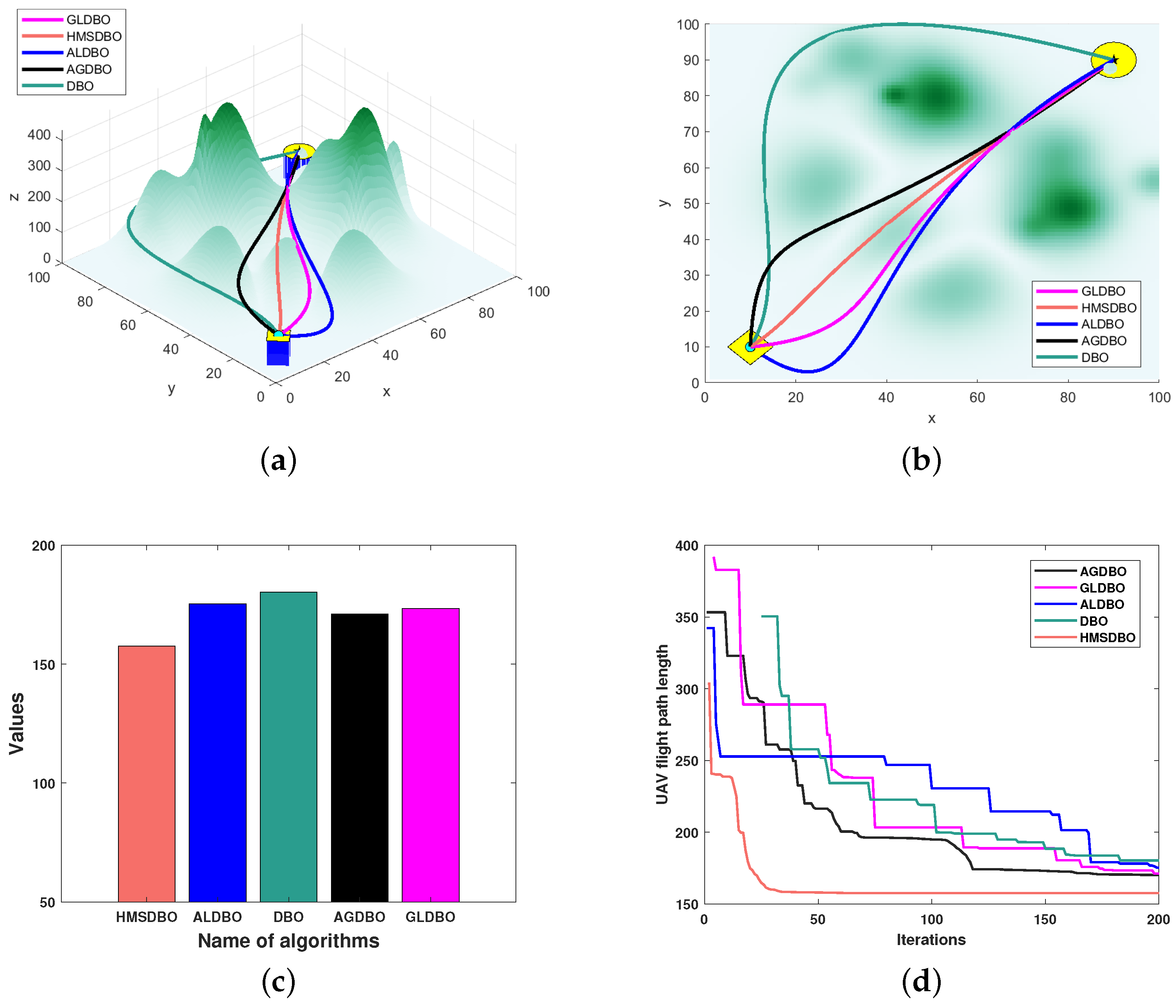
A novel HMSDBO algorithm is proposed for the 3D path planning of agricultural UAVs, significantly enhancing the efficiency and accuracy of path searches. The algorithm reduces path lengths, improves path smoothness, and adapts effectively to environmental changes and obstacles, thereby meeting the real-time navigation requirements in complex environments.
(2)
An innovative Latin hypercube sampling method (LHS) is developed for population initialization, greatly improving the algorithm’s global search capability and promoting diversity within the population. Additionally, a new golden sine strategy and hybrid adaptive weighting strategy are introduced to address the limitations during the global search and local refinement phases. These innovations enhance convergence speed, robustness, and prevent the algorithm from becoming trapped in local optima.
(3)
A new 3D path planning model is introduced to accurately simulate the actual flight environment, substantially improving system accuracy. This model integrates key factors such as obstacle avoidance, path smoothness, and path length, while incorporating an innovative objective function that optimizes routes and effectively balances flight costs.
(4)
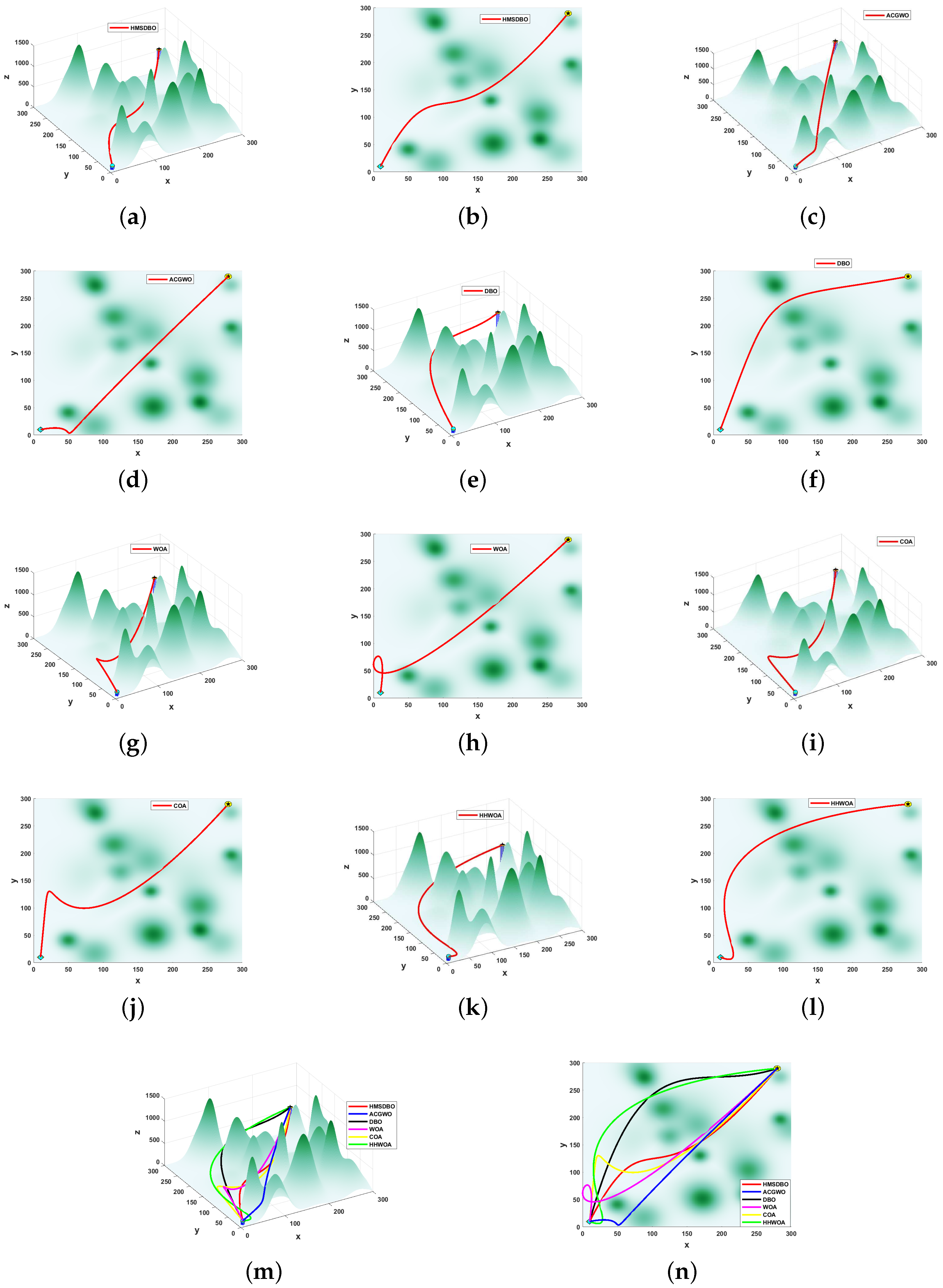
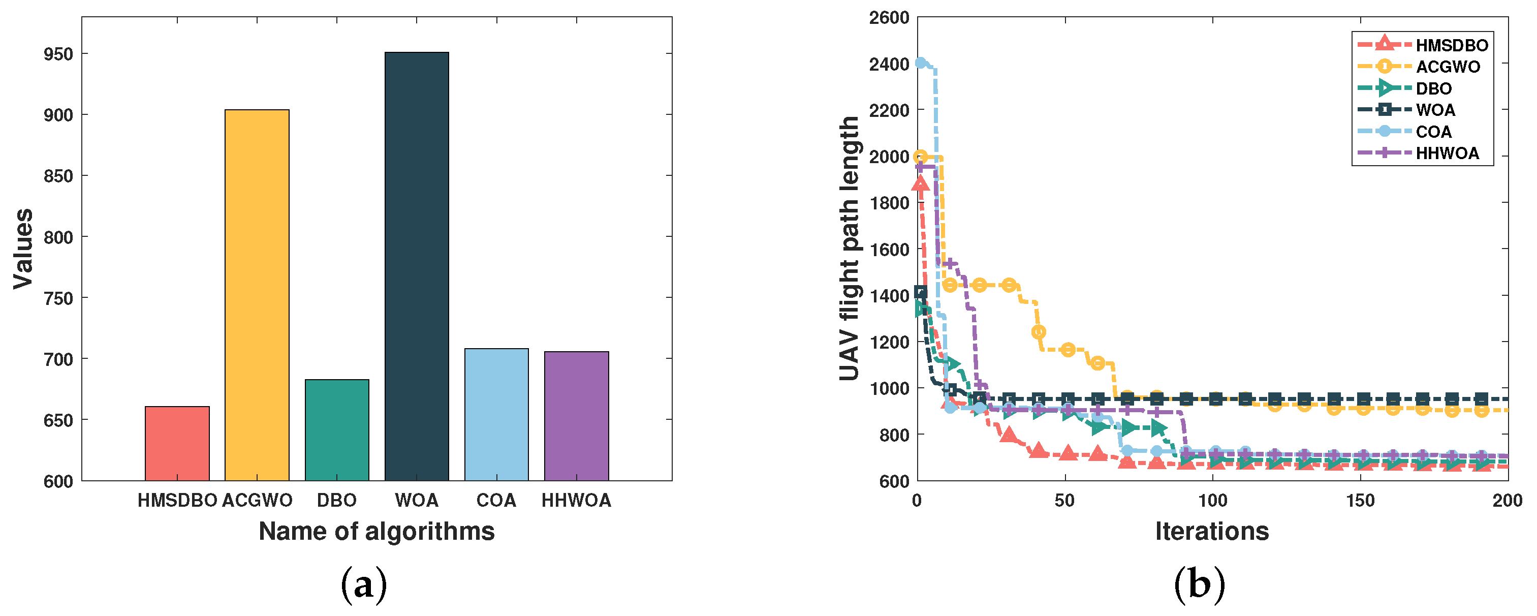
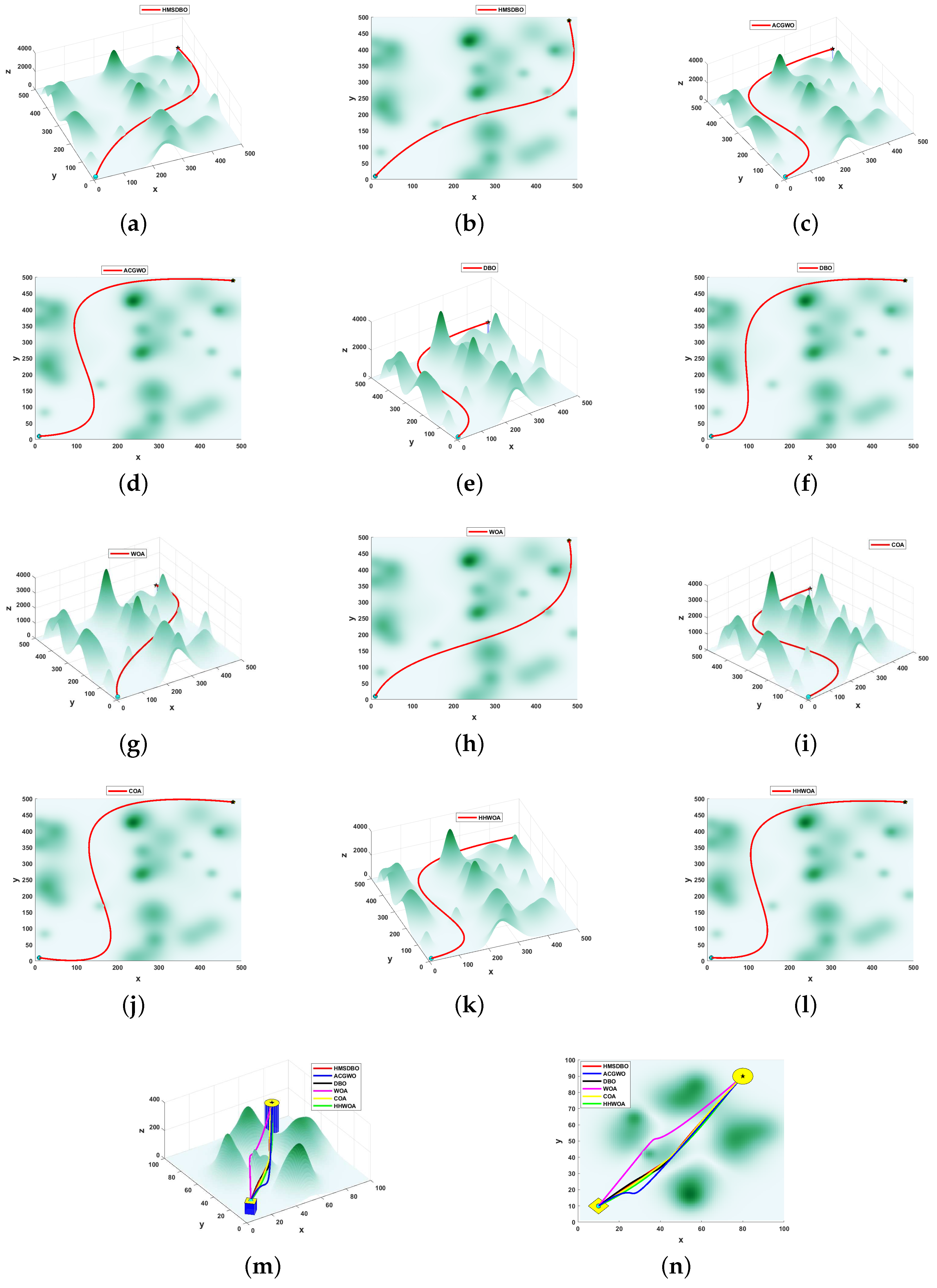
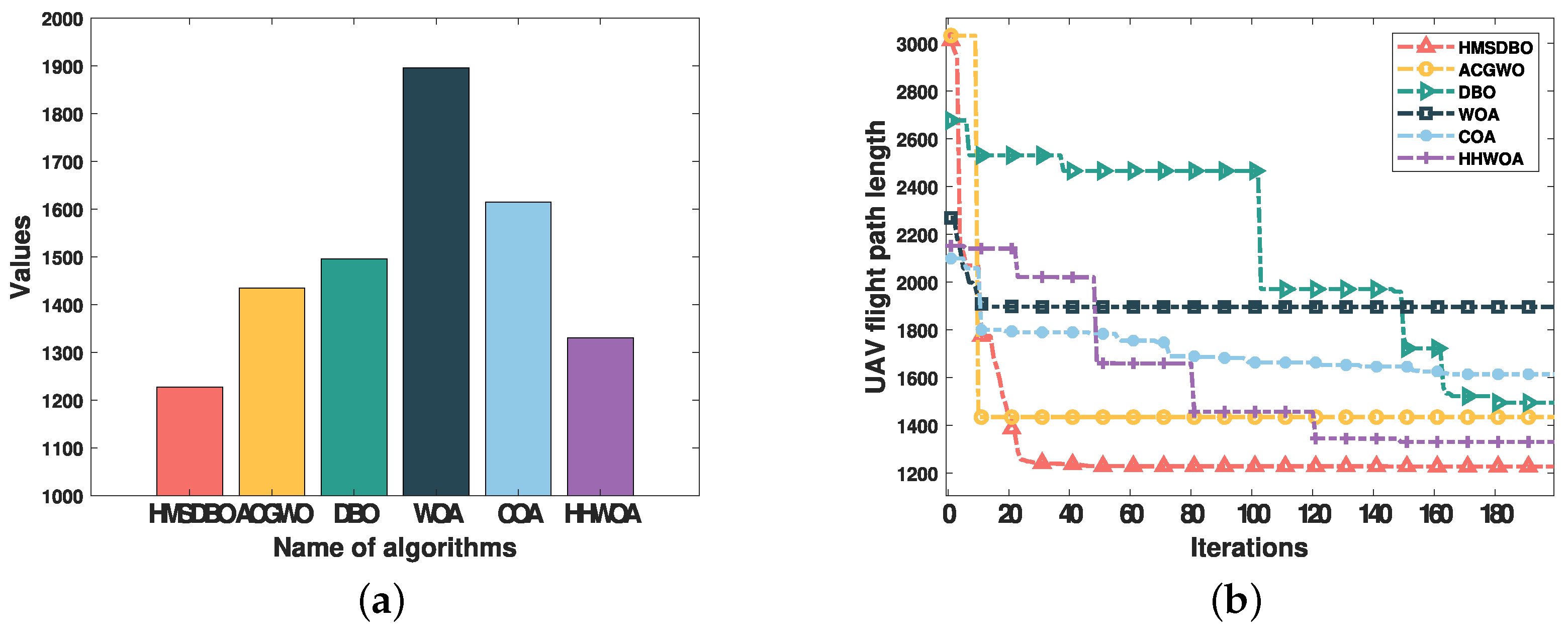
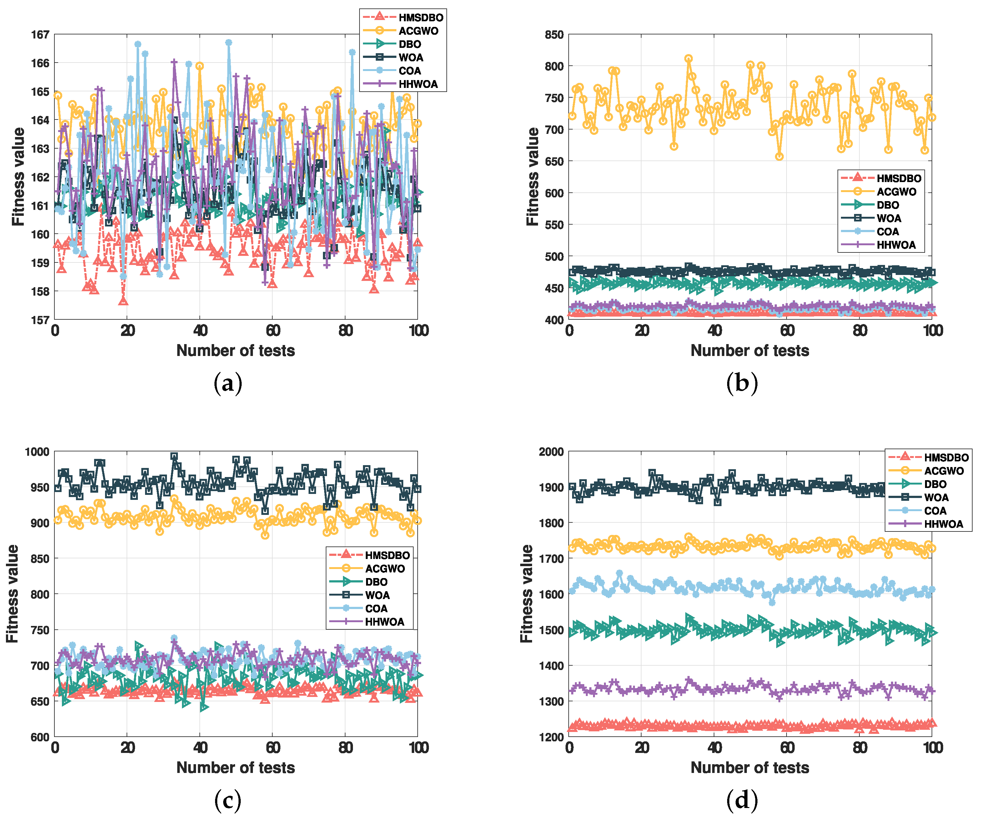
A comprehensive set of simulation-based validations is designed to evaluate the performance of HMSDBO in UAV path planning optimization. Simulation results demonstrate that HMSDBO outperforms several algorithms, including ACGWO, DBO, WOA, COA, and HHWOA. Specifically, HMSDBO reduces path lengths by at least 4.2% while significantly enhancing path smoothness.
This paper is organized as follows: Section 2 reviews the research results in related fields; Section 3 elaborates the 3D UAV path planning model; Section 4 describes the specific flow of the HMSDBO algorithm; Section 5 presents the process of the simulation experiments and analyzes the experimental results in-depth; and, finally, Section 6 summarizes the main conclusions of this paper.

2. Related Work

In the field of agricultural UAV path planning, numerous studies have focused on developing algorithms capable of generating efficient and reliable 3D paths in complex environments [23]. These path planning methods typically need to meet multiple constraints, including minimizing energy consumption, reducing path length, enhancing obstacle avoidance capabilities, and achieving optimal task completion time. In recent years, population intelligence algorithms have emerged as one of the mainstream approaches in UAV path planning due to their outstanding performance in solving complex optimization problems.

2.1. Traditional Path Planning Algorithms

Conventional path planning techniques encompass the A* algorithm, Dijkstra’s algorithm, and RRT (Rapid Randomized Tree) algorithm. Jinchao Chen et al. [24] developed an exact formulation utilizing Mixed-Integer Linear Programming (MILP) to thoroughly explore the solution space for UAV models and operational areas. Subsequently, they proposed an enhanced A* algorithm aimed at generating optimal flight paths for UAVs by refining both the evaluation function and the node selection strategy. Xiong Bai et al. [25] proposed an A- and DWA-based path planning algorithm designed to optimize the paths of unmanned aerial vehicles (UAVs) while improving safety and speed. The algorithm effectively improves path efficiency and safety by improving A and adaptively adjusting the evaluation function of DWA, and experimental results show that it performs well in shortening the path length and reducing the planning time. Dilip Mandloi et al. [26] comparatively analyzed the path planning performance of algorithms such as A*, Theta, and Lazy Theta in 3D environments, with a focus on the performance of the capability of these algorithms for obstacle avoidance and path optimization in the context of unmanned aerial vehicles (UAVs) when moving from the starting point to the endpoint. The study tested their performance in scenarios with different dimensions and obstacle complexity and evaluated the performance of the algorithms by two metrics: computation time and path length. Elaf Dhulkefl et al. [27] sought to establish the optimal path for the UAV to arrive at the target point while avoiding obstacles, utilizing Dijkstra’s algorithm for this purpose. The study developed a MATLAB program to evaluate the arrival time of the UAV and perform simulations. In the study, obstacles were defined for buildings of different heights and widths and 2D and 3D models were constructed assuming that the UAV was flying at a certain height. In addition, flight tests were conducted based on route planning in real applications, and data such as battery consumption, speed, and travel were examined. Jun Guo et al. [28] introduced a data-driven path planning method for UAVs in hostile environments, the Feedback Rapid Exploratory Random Treestar Algorithm (FRRT*). The algorithm’s goal is to establish a risk-constrained shortest path from the origin to the target point, taking into account the characteristics of the defense system. FRRT* employs situational information to regulate the expansion of the random tree, thereby enhancing planning efficiency through the integration of a data-driven risk network and a feedback mechanism. Jiaming Fan et al. [29] introduced a UAV trajectory planning approach that combines the PFRRT algorithm with a target bias strategy to address the issue of slow convergence typically associated with RRT. The approach decreases the overall path cost using a dichotomous strategy to create new parent nodes for newly formed nodes located near obstacles. The improved artificial potential field (APF) enhances the attractive and repulsive forces to promote the expansion of the random tree in the direction of the target point and solves the local minimum problem.

2.2. Group Intelligence Algorithms for Path Planning

To address the limitations of traditional algorithms, researchers have introduced various swarm intelligence optimization algorithms, including the Whale Optimization Algorithm (WOA), Gray Wolf Optimization (GWO), and Dung Beetle Optimization (DBO). These algorithms achieve globally optimal pathfinding by mimicking the cooperative behaviors observed in natural ecosystems. Mehmet Enes Avcu et al. [30] proposed a meta-heuristic swarming algorithm framework to tackle the challenging problem of collision avoidance for micro UAVs. In their study, WOA was applied to solve collision avoidance issues in cluttered environments, and its effectiveness was demonstrated through simulations. Binggang Yu et al. [31] developed a novel whale optimization algorithm enhanced with elements of the simulated annealing process, referred to as the Simulated Annealing–Whale Optimization Algorithm (SA-WOA). This innovative approach integrates adaptive weights to improve the Levy flight mechanism, refines the Metropolis criterion, and applies a dynamic thermoregulation strategy during the simulated annealing phase. Additionally, a path-smoothing step using non-uniform rational B-spline (NURBS) curves is incorporated to optimize the generated paths. Xinyu Liu et al. [32] introduced a collaborative enhanced Gray Wolf Optimization Algorithm called the Multi-Mechanism Collaborative Improved Gray Wolf Optimization Algorithm (NAS-GWO), designed specifically for addressing trajectory planning challenges in agricultural UAVs. This algorithm employs multiple mechanisms to improve optimization performance in trajectory planning. A boundary constraint handling mechanism updates the position of any gray wolf that exceeds the designated limits, preserving optimal individual information and enhancing search accuracy. Furthermore, a Gaussian mutation strategy and a spiral function act as perturbation mechanisms, helping the algorithm escape local optima. To balance exploration and exploitation, an enhanced Sigmoid function is employed as a nonlinear convergence factor. Wei Zhang et al. [33] proposed an improved Adaptive Gray Wolf Optimization (AGWO) algorithm for 3D path planning in UAV supply delivery to earthquake-stricken areas. This algorithm introduces an adaptive convergence factor and a weighting factor to update individual positions. Its effectiveness was verified through simulations, where it was combined with digital elevation maps and an equivalent mountain threat model to construct an environment map. A performance evaluation function was established by fitting and calculating the trajectory length. Qianwen Shen et al. [34] proposed a multi-strategy augmented dung beetle optimizer (MDBO) for 3D UAV path planning. This algorithm dynamically generates reflective solutions to allow the broader exploration of the search space, helping particles escape local optima. A Levy distribution is employed to handle out-of-bounds particles, while the thief beetle’s update phase is optimized using two crossover operators to accelerate convergence and balance exploration and exploitation. Lixin Lyu et al. [35] introduced a multi-strategy augmented dung beetle optimization algorithm (IDBO) for UAV 3D path planning. The algorithm uses cubic chaos mapping to initialize the population, thereby improving diversity, and incorporates a global exploration strategy to enhance information exchange and reduce parameter dependency. An adaptive t-distribution mechanism is used to adjust the positions of dung beetles, striking a balance between exploration and exploitation.

2.3. Motivation

In this section, the characteristics and limitations of previous studies are summarized and analyzed. The conclusions are outlined as follows.
Limitations of Traditional Path Planning Algorithms: Traditional path planning algorithms face several significant drawbacks. First, they are computationally inefficient, especially in complex environments or large-scale problems, where computation time increases substantially and real-time performance becomes inadequate. Additionally, these algorithms often struggle with scalability, as their performance deteriorates with an increasing number of obstacles or a larger search space. Furthermore, they lack flexibility, making it difficult to adapt to dynamic changes in the environment.
Challenges of Swarm Intelligence Algorithms: While swarm intelligence algorithms are effective in exploring solution spaces, they also exhibit distinct shortcomings in path planning. These algorithms often converge slowly, prolonging the optimization process required to find an ideal solution. Moreover, they are prone to falling into local optima, which limits their ability to identify globally optimal paths. Many swarm intelligence methods are also highly sensitive to parameter settings, necessitating extensive tuning and experimentation. This sensitivity complicates their practical application, particularly in dynamic environments where adaptability is crucial. Furthermore, the generated paths may lack smoothness and coherence, reducing efficiency and safety in real-world scenarios.
In summary, although both traditional and swarm intelligence algorithms have their respective strengths, they face significant challenges and limitations. To address these issues, this paper proposes an HMSDBO to achieve more efficient path planning. By integrating multiple optimization strategies, this algorithm enhances search speed and global optimization capability, effectively overcoming the limitations of traditional path planning algorithms. Additionally, a new 3D agricultural UAV path planning model is introduced, designed to meet the obstacle avoidance requirements of complex environments while optimizing path length and flight smoothness. This paper presents an efficient solution to the UAV path planning problem in complex environments by incorporating advanced algorithmic techniques for faster and more accurate path planning.

3. Three-Dimensional UAV Path Planning Model Design

In agricultural UAV path planning research, it is crucial to accurately simulate obstacles in complex environments. This simulation not only aids in confirming the effectiveness of the path planning algorithm but also enhances its adaptability and resilience in real-world applications. In order to better simulate the flight environment of UAVs in complex terrain, this paper designs a three-dimensional environment model that can reflect a variety of terrain features. In path planning, the environment model designed according to the geographic location information trajectory is defined in a right-angle coordinate system of size 100 × 100 × 400, 200 × 200 × 1000, 300 × 300 × 1500, 500 × 500 × 4000, respectively. The obstacle region is modeled as a peak model in the Cartesian coordinate system. The following provides the mathematical expression for the peak model. In Table 1, the parameters employed in this model are detailed.
Z ( x , y ) = i = 1 n h i e x p [ ( ( x x i ) 2 x s i 2 + ( y y i ) 2 y s i 2 ) ]
where ( x i , y i ) is the center coordinate of the i-th peak, h i is the height parameter of the peak, x s i and y s i are the scale control parameters of the i-th peak on the x axis and y axis, respectively, and n denotes the number of peaks.

3.1. Flight Path and Smoothing

The flight path is composed of a straight line segment formed by connecting the position points of the ith dung beetle, and the path includes a starting point P s ( x s , y s , z s ) , an end point P e ( x e , y e , z e ) , and a position point P i j ( x i j , y i j , z i j ) of each dung beetle individual in the path, where j = 1 , 2 , 3 , and n stands for the number of dung beetle individuals. The starting point, end point, and these location points together form the complete flight path, so the path can be represented as p s , p i 1 , p i 2 , , p i n 1 , p e . By connecting these points sequentially, the resulting flight path is a folded line. In UAV path planning, the generated initial paths are often irregular, curved, or sharply turned due to the complex terrain and obstacles in the environment. This situation may not only lead to increased instability and energy consumption during the flight, but also affects the flight safety of the UAV. Therefore, smoothing the planned path is an essential step [36,37]. In order to reduce the length of the flight path and generate smoother flight trajectories, this paper utilizes the cubic B-spline interpolation technique [38,39] to interpolate the discrete path points so as to draw a smooth flight path curve.

3.1.1. Path Smoothing Basis Functions

Given n + 1 control points P i ( i = 0 , 1 , 2 , , n ) in the i-th segment of the flight path, n B-spline segments can be generated:
P i ( λ ) = i = 0 n P i B i , h ( λ )
where P i denotes the control point of the flight path and B i , k ( λ ) denotes the spline basis function. The common B-spline basis function usually uses the Cox–deBoor recursive formula, as shown in Equation (3).
B i , 0 ( g ) = 1 , g i g < g i + 1 0 , o t h e r w i s e B i , h ( g ) = g g i g i + h g i B i . h 1 ( g ) + g i + h + 1 g g i + h + 1 g i + 1 B i + 1 , h 1 ( g ) d e f i n e 0 0 = 0
where h is a power of the B-spline function with a total of n + 1 dung beetle location points. When h = 1 , the primary basis function is obtained from Equation (3) as
B i , 1 ( g ) = g g i g i + 1 g i B i , 0 ( g ) + g i + 2 g g i + 2 g i + 1 B i + 1 , 0 ( g ) = g g i g i + 1 g i , g i g < g i + 1 , g i + 2 g g i + 2 g i + 1 , g i + 1 g < g i + 2 , 0 , otherwise .
where B i + 1 , 0 ( g ) can be derived from N i , 0 ( g ) . When h = 2 , the quadratic basis functions can be derived from Equations (3) and (4).
B i , 2 ( g ) = g g i g i + 2 g i B i , 1 ( g ) + g i + 3 g g i + 3 g i + 1 B i + 1 , 1 ( g ) = ( g g i ) 2 ( g i + 1 g i ) ( g i + 2 g i ) , g i g < g i + 1 , g g i g i + 2 g i · g i + 2 g g i + 2 g i + 1 + g i + 3 g g i + 3 g i + 1 · g g i + 1 g i + 2 g i + 1 , g i + 1 g < g i + 2 , ( g i + 3 g ) 2 ( g i + 3 g i + 1 ) ( g i + 3 g i + 2 ) , g i + 2 g < g i + 3 , 0 , otherwise .
where B i + 1 , 1 ( g ) can be derived from B i , 1 ( g ) . When h = 3 , Equation (6) can be derived from Equations (3) and (5).
B i , 3 ( g ) = g g i g i + 3 g i B i , 2 ( g ) + g i + 4 g g i + 4 g i + 1 B i + 1 , 2 ( g ) = ( g g i ) 3 ( g i + 1 g i ) ( g i + 2 g i ) ( g i + 3 g i ) , g i g < g i + 1 , ( g g i ) 2 ( g i + 2 g ) ( g i + 3 g i ) ( g i + 2 g i ) ( g i + 2 g i + 1 ) + g i + 3 g ( g i + 3 g i + 1 ) ( g i + 3 g i ) ( g i + 2 g i + 1 ) + ( g g i + 1 ) 2 ( g i + 4 g ) ( g i + 4 g i + 1 ) ( g i + 3 g i + 1 ) ( g i + 2 g i + 1 ) , g i + 1 g < g i + 2 , ( g g i ) ( g i + 3 g ) 2 ( g i + 3 g i ) ( g i + 3 g i + 1 ) ( g i + 3 g i + 2 ) + ( g i + 4 g ) ( g g i + 1 ( g i + 3 g ) ) ( g i + 4 g i + 1 ) ( g i + 3 g i + 1 ) ( g i + 3 g i + 2 ) + ( g i + 4 g ) 2 ( g g i + 2 ) ( g i + 4 g i + 1 ) ( g i + 4 g i + 2 ) ( g i + 3 g i + 2 ) , g i + 2 g < g i + 3 , ( g i + 4 g ) 3 ( g i + 4 g i + 1 ) ( g i + 4 g i + 3 ) , g i + 3 g < g i + 4 0 , otherwise .
In the B-spline curve formulation, the value of h is used to indicate the smoothness of the curve. The curve smoothing of the flight path is achieved by a uniform B-spline basis, and since the spacing between the nodes of the uniform spline basis is equal, g i + 1 g i = h . In particular, when g i = i , h = 1 . This can be expressed as
g g i = λ , g i g < g i + 1 g g i + 1 = λ , g i + 1 g < g i + 2 g g i + 2 = λ , g i + 2 g < g i + 3 g g i + 3 = λ , g i + 3 g < g i + 4
where λ takes values between [0, 1], which can be brought into Equation (6) to obtain Equation (8).
B i , 3 ( λ ) = 1 6 λ 3 1 6 ( 3 λ 3 + 3 λ 3 + 3 λ + 1 ) 1 6 ( 3 λ 3 6 λ 2 + 4 ) 1 6 ( 1 λ ) 3
The i-th segment of path points on the UAV path is assembled into a set R. The set R contains n + 1 control points P 0 , P 1 , P 2 , , P n . When n = 3 and h = 3 , i.e., a cubic B-spline curve consisting of four control points P 0 , P 1 , P 2 , P 3 is formed, and the variable is x. At this point, Equation (2) transforms to
P i ( λ ) = i = 0 3 P i B i , 3 ( x )
Substituting Equation (8) into Equation (9), the cubic spline interpolation curve equation for segment i can be obtained as follows:
P i ( x ) = B 0 , 3 ( x ) P 0 + B 1 , 3 ( x ) P 1 + B 2 , 3 ( x ) P 2 + B 3 , 3 ( x ) P 3 = [ B 0 , 3 ( x ) , B 1 , 3 ( x ) , B 2 , 3 ( x ) , B 3 , 3 ( x ) ] P 0 P 1 P 2 P 3 = 1 6 [ 1 x x 2 x 3 ] 1 4 1 0 3 0 3 3 3 6 3 0 1 3 3 1

3.1.2. Curve Interpolation

Equation (10) is determined by four control points, let the coordinates of the control points be ( X i , Y i , Z i ) (where i = 1 , 2 , , n i = 1 , 2 , , n ), and the coordinates of any point after curve interpolation ( X g , Y g , Z g ) are expressed as
X g = i = 0 m X i B i , h ( g ) Y g = i = 0 m Y i B i , h ( g ) Z g = i = 0 m Z i B i , h ( g )

3.1.3. Constraints

The constraints are set up to ensure that the UAV flight path lies within the designated airspace and can effectively avoid obstacles. Therefore, two key constraints are proposed.
  • To ensure that the flight path remains within the specified airspace, the following constraints must be met:
0 x i x m a x 0 y i y m a x , i = 1 , 2 , · · · , n 0 z i z m a x
  • To avoid the collision of the drone with obstacles within the terrain, it needs to be satisfied:
Z i > Z ( x i , y i ) , i = 1 , 2 , · · · , n

3.1.4. Energy Consumption Model

UAV flight energy consumption consists of two parts: flight power consumption and landing power consumption. The formula for calculating flight power consumption is shown below.
E T = 1 2 C D S D v 3 + m 2 D b 2 v
where E T is the power required for flight (W); C D is the air resistance coefficient, generally take C D = 0.546; S is the windbreak area, take S = 1.2 m2; m is the mass, take m = 120 kg; D is the air density, take D = 1.39 kg/m3; b is the width of the UAV, take b = 8.7 m; v is the relative speed of the UAV in the air, assuming that the UAV flying at a constant velocity, then v = 17 m/s.
The formula for calculating the UAV takeoff and landing power consumption is shown below.
E g = T 3 2 2 D s
where E g is the power required for the vertical takeoff and landing of the UAV ( W ) , T is the thrust ( N ) , T = m g , and g is the acceleration of gravity, g = 9.8 N/kg. The specific principles of the UAV energy consumption model have been described in detail by scholars.

3.1.5. Objective Function

The objective function of the UAV flight path consists of three main parts, which are the total flight distance of the UAV, the cost of avoiding obstacles, and the cost of flying within the specified boundary. The expression of the overall objective function of the UAV is as follows:
m i n ( C ) = m i n ( T c + V c + D c + E g )
where T c represents the cost of the UAV when it bypasses an obstacle, V c refers to the total range cost of the UAV flight, and D c denotes the cost of the UAV when it flies within a defined boundary.
The terrain cost T c is mainly used to ensure that the UAV flight path avoids obstacles, which is achieved by adjusting the size of the T c value. When the UAV flight height z i is higher than the height of the obstacles in the terrain z 2 ( x i , y i ) , set T c = 0 ; and when z i is lower than the height of the obstacles z 2 ( x i , y i ) , set T c = . In this way, the summation can ensure that the UAV’s flight path can effectively avoid obstacles such as mountain peaks. The expression is as follows:
T c = i = 1 n T c , T c 0 = 0 T c i = 1 , Z i > Z ( x i , y i ) , otherwise
The overall range cost V c primarily serves to quantify the total distance traveled by the UAV from the initial point to the final destination, the sum of the individual arc segments L i . If the entire trajectory consists of n segments, then the expression for the total range cost is
V c = i = 1 n 1 L i
L i = ( x i + 1 x i ) 2 + ( y i + 1 y i ) 2 + ( z i + 1 z i ) 2
D c = i = 1 n D c i , D c 0 = 0 D c i = 0 , x i [ 0 , x max ] y i [ 0 , y max ] z i [ 0 , z max ] , otherwise

4. Three-Dimensional Agricultural UAV Path Planning Based on HMSDBO

In 3D agricultural UAV path planning, optimizing the flight path is crucial for achieving efficient and safe mission execution. As UAV technology continues to evolve rapidly, addressing the challenges of path planning in complex environments has become increasingly important. The Dung Beetle Optimization (DBO) algorithm employs an effective global search and local optimization strategy by simulating five behaviors and four sub-populations of dung beetles. While the algorithm demonstrates advantages such as rapid convergence, high accuracy, and strong stability, it also has certain limitations. First, the initial population in the DBO algorithm is generated using a random distribution, which can result in an uneven distribution of individuals within the search space. This irregularity negatively impacts the global search capability of the algorithm. Second, the DBO algorithm often struggles to maintain a balance between global exploration and local exploitation, leading to a tendency to become trapped in local optima. This limitation reduces its effectiveness in identifying the global optimal solution. To address these issues, this paper proposes three strategies to enhance the DBO algorithm and improve its performance.

4.1. Dung Beetle Optimization Algorithm

(1)
Dung Beetle Roller
Dung beetles roll dung balls for the purpose of laying eggs, providing nutrients for their offspring, and stockpiling food. In the process, dung beetles rely on celestial cues to keep the dung ball rolling path straight. Within the search space, the dung beetle advances in a specified direction, resulting in an update to its position as it rolls the dung ball. This movement can be mathematically represented as follows.
x i ( t + 1 ) = x i ( t ) + a · k · x i ( t 1 ) + b · Δ x
Δ x = | x i ( t ) X w |
where t denotes the current iteration number; x i ( t + 1 ) is the position of the ith dung beetle at the t + 1 -th iteration; x i ( t ) is the position information at the t-th iteration; x i ( t 1 ) denotes the position information at the t-th iteration; a is the natural coefficient, which denotes whether the dung beetles deviate from the original direction or not, and takes the value of −1 or 1 which is determined based on the probability; k is the deflection coefficient constant with the range of k ( 0 , 0.2 ] ; η is a random number between ( 0 , 1 ) , φ denotes the probability that the dung beetle encounters an obstacle, and b is a constant with the range of ( 0 , 1 ) ; Δ x the simulated change of the light intensity, and X w is the global worst position.
When a dung beetle faces an obstacle blocking its path, it employs a dancing behavior to explore and choose a different route to continue its journey. The formula for the rolling dung beetle to dance to update its position is shown below.
x i ( t + 1 ) = x i ( t ) + tan ( θ ) | x i ( t ) x i ( t + 1 S ) |
where θ [ 0 , π ] , the rolling dung beetle does not update its position when θ = 0 , π / 2 or π .
(2)
Breeding Dung Beetles
Dung beetles select appropriate habitats for laying their eggs to guarantee the safety and survival of their young. Inspired by this behavior, a boundary selection strategy has been developed to mathematically represent the breeding grounds of female dung beetles, described by the following expression:
L b * = m a x [ X * · ( 1 R ) , L b ]
U B * = m a x [ X * · ( 1 + R ) , U b ]
where U b * and L b * indicate the maximum and minimum boundaries of the spawning region, respectively; X * refers to the present local optimum position; R = 1 t / T , where T represents the total allowed iterations; U b and L b are the upper and lower limits of the optimization task, respectively.
B t ( t + 1 ) = X * + b 1 · [ B t ( t ) L b * ] + b 2 [ B t ( t ) U b * ]
where B i ( t + 1 ) denotes the position of the i-th breeding dung beetle in the t + 1 -st iteration, and B i ( t ) is its position at the t-th iteration; b 1 and b 2 are 1 × D independent random vectors, and D denotes the dimension of the optimization problem.
(3)
Dung beetle
When dung beetles grow up, they leave their spawning area in search of food, at which point they are referred to as baby dung beetles. To simulate their foraging behavior, an optimal foraging area was established with boundaries defined as follows:
L b b = m a x [ X b · ( 1 R ) , L b ]
U b b = m i n [ X b · ( 1 R ) , U b ]
where U b and L b denote the upper and lower bounds of the optimal foraging area, respectively, and X b is the global optimum location. Therefore, the formula for updating the position of the smaller dung beetle is
x i ( t + 1 ) = x i ( t ) + C 1 · [ x i ( t ) L b b ] + C 2 [ x i ( t ) U b b ]
where C 1 is a random number generated according to the normal distribution; and C 2 is a random vector of ( 0 , 1 ) .
(4)
Stealing Dung Beetles
According to Equation (30), it can be seen that the thief dung beetle will compete for food near the global optimal position X b . As the iteration proceeds, the position of the thief dung beetle is updated by Equation (30):
x i ( t + 1 ) = X b + S · g · ( | x i ( t ) X * | + | x i ( t ) X b | )
where S is a constant; and g is a randomly generated 1 × D vector based on a normal distribution.

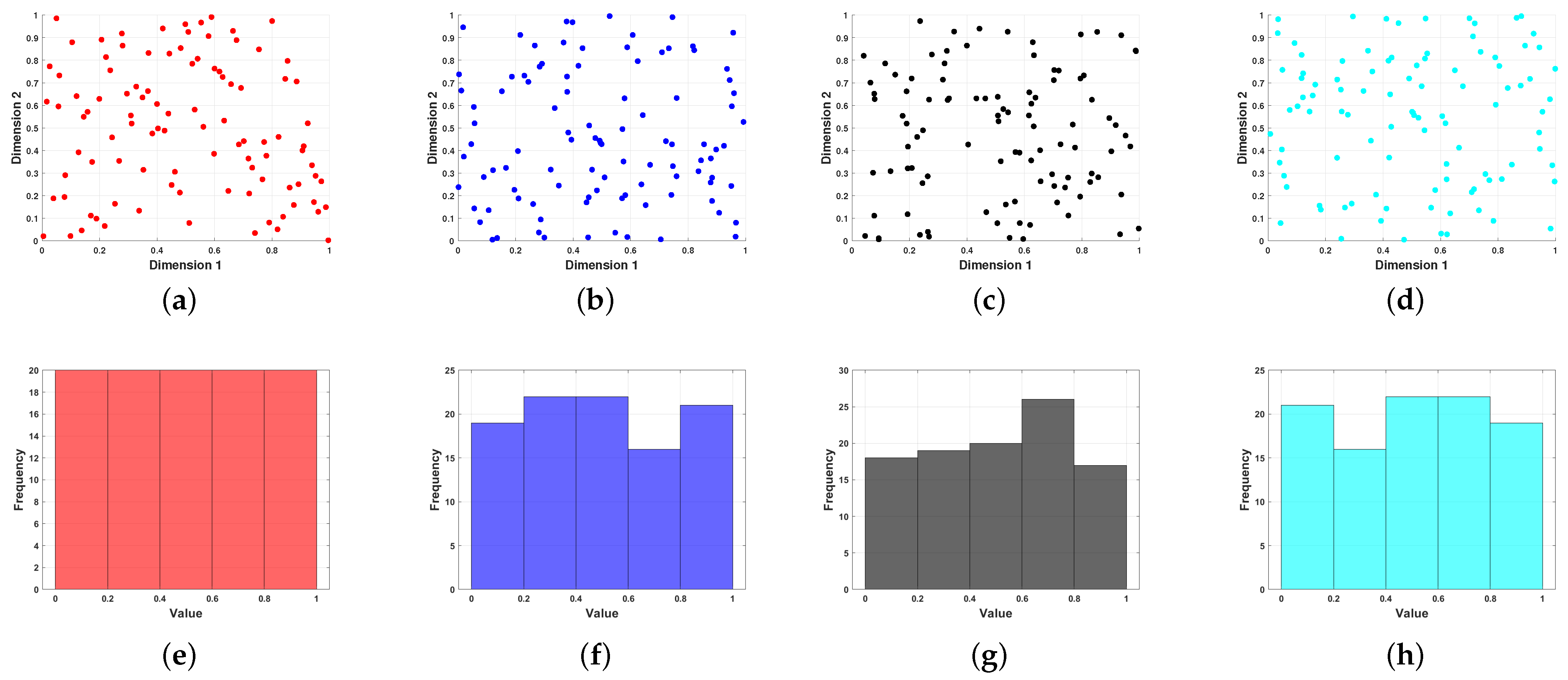
4.2. Latin Hypercube Sampling Strategy for Initializing Populations

LHS is a statistical method for the random sampling of multidimensional variables, particularly suited for computerized experimental design. In the context of agricultural UAV path planning, LHS can be applied to optimize the initialization of the algorithm’s population by ensuring a more diverse and evenly distributed set of initial solutions in the search space. This is critical in improving the algorithm’s global search capability and preventing premature convergence caused by clustering of samples in specific regions—a common issue in traditional random sampling methods.
The process begins by defining the number of variables as n, which, in the case of agricultural UAV path planning, could represent key dimensions such as flight altitude, path length, or obstacle avoidance parameters. Each variable is divided into m, equal probability intervals. For the j-th variable ( j [ 1 , n ] ) and the i-th sample point ( i [ 1 , m ] ) , the sample point component x i j generated by Latin Hypercube Sampling can be calculated using the following equation. By employing LHS in the initialization phase of the path planning algorithm, the agricultural UAV can explore a broader range of possible paths more effectively, ensuring better adaptability to dynamic and complex environments. This ultimately improves the UAV’s ability to avoid obstacles, optimize flight efficiency, and minimize path length in challenging agricultural settings.
X i j = π i j + U i j m
where x i j denotes the jth component value of the ith sample point; π is the i-th element of the sequence 0 , 1 , , m 1 in the sequence 0 , 1 , , m 1 , which is used to determine the interval in which the sample point is located, and U i represents a random value uniformly distributed within the range [ 0 , 1 ) , which is used to randomly generate the sample point in the selected interval.
Figure 1a–h represent comparative experiments to verify the effectiveness of the Latin hypercube sampling initialization. The lenticular reverse learning initialization, the random initialization, and the original initialization of the sand cat algorithm are compared, respectively.

4.3. Gold Sine Strategy

Dung beetles exhibit their rolling behavior in two distinct modes: obstructed and unobstructed. During unobstructed rolling, the dung beetle’s location within the search space adjusts as the sunlight’s intensity shifts. The golden sine algorithm is a meta-heuristic algorithm proposed by Tanyildizi et al. in 2017 [40]. With the golden sine strategy, HMSDBO is able to dynamically adjust its search behavior at different stages, making global exploration and local exploitation more balanced, thus improving the optimization performance. In this paper, the golden sine method is incorporated into the dung beetle optimization algorithm as a replacement for the dung beetle tangent dance. The position update rules for the rolling dung beetle are detailed in Equations (33) and (34).
X i ( t + 1 ) = X i ( t ) + a · k · X i ( t + 1 ) + b Δ x , ξ < S T ,
X i ( t + 1 ) = X i ( t ) | sin R 1 | R 2 sin R 1 | θ 1 X b ( t ) θ 2 X i ( t ) | , ξ S T
α ( λ ) = 1 , η > φ 1 , η < φ
θ 1 = π + 2 π ( 1 τ )
θ 2 = π + 2 π τ
where η is a random number in the range of ( 0 , 1 ) , ψ denotes the probability that a dung beetle encounters an obstacle, λ ( 0 , 1 ) , τ the golden section, τ = ( / 5 1 ) / 2 , and ξ represents a random value within the range of [0, 1]. S T signifies a random number that also falls within the interval of [ 0 ,   1 ] .

4.4. Hybrid Adaptive Weighting Strategy

The location of the brood ball is modified in response to changes in the spawning area, and its position is updated in the manner shown in Equation (37).
X i ( t + 1 ) = ( r a n k i ( t ) 1 ) p o p 1 · X * + b 1 · ( X i ( t ) L b * ) + b 2 · ( X i ( t ) U b * )
To dynamically modify the algorithm’s search range and ensure a balanced search capability during both pre- and post-iteration phases, adaptive inertia weights are introduced in the position update of the stealing dung beetle in this paper. The position adjustment approach for the stealing dung beetle is outlined in Equation (38).
ω = cos ( t 2 T × π ) + ( ω m a x + ω m i n 4 )
where w m a x represents the starting inertia weight, set at 0.96; w m i n denotes the inertia weight after reaching the maximum number of iterations, valued at 0.2.
X i ( t + 1 ) = [ r a n k i ( t ) 1 ] p o p 1 · X b + S · r · | x i ( t ) ω · X * | + | x i ( t ) X b |
where x ( t ) denotes the position of the i-th stealing dung beetle at the t-th iteration, r is a random vector of size 1 × D obeying a normal distribution, and S is a constant.
Figure 2 represents the flowchart of the algorithm of HMSDBO.
The pseudocode for the HMSDBO algorithm is shown in Algorithm 1.
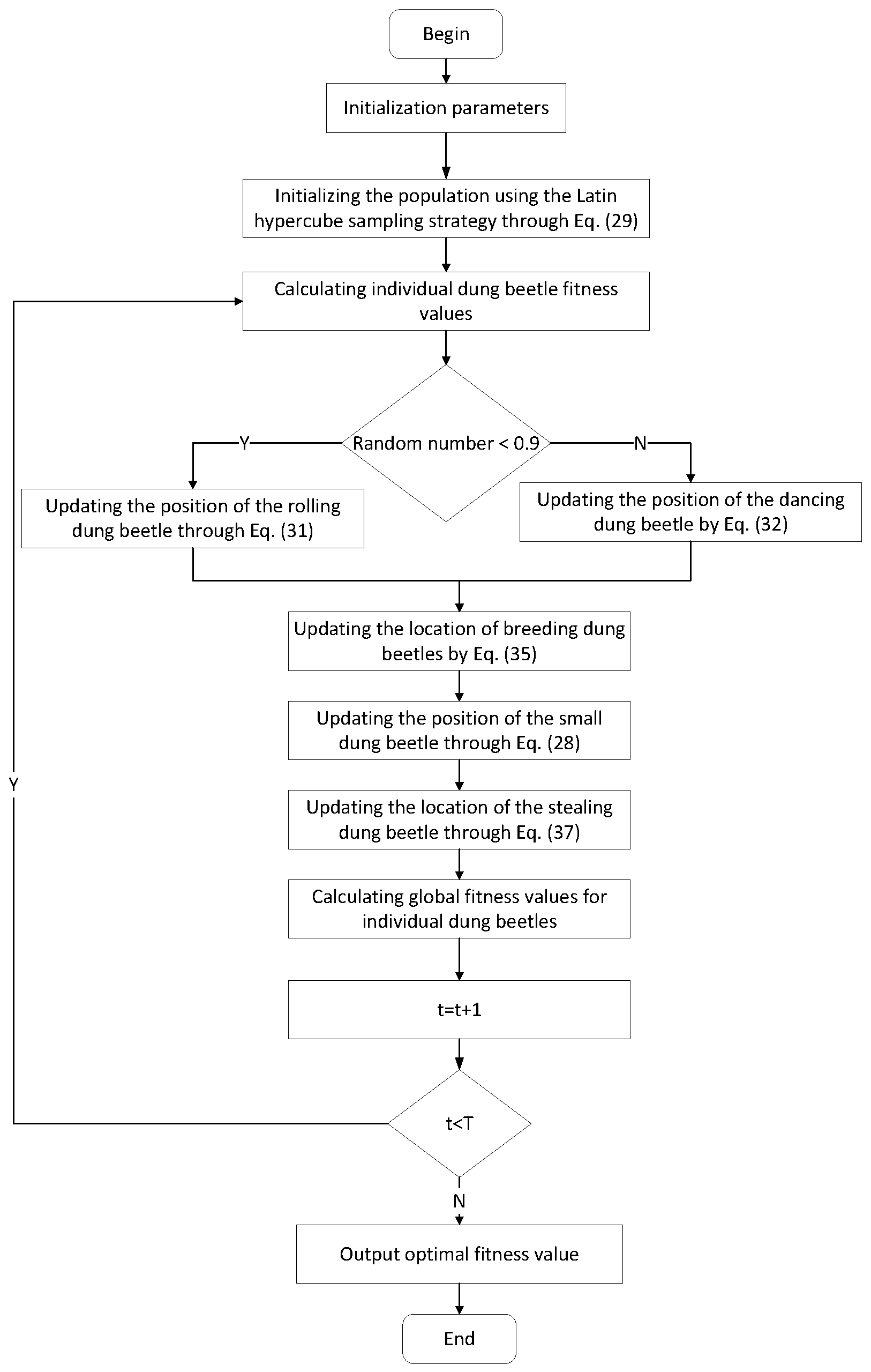
Algorithm 1: Algorithm flowchart of HMSDBO
Input: Population size n
Maximum number of iterations T
Current iteration t
Starting point x
End point y
Output: Optimal fitness value
Initialize parameters
Perform Latin hypercube sampling for initializing populations
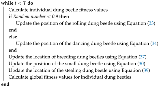
Agriculture 15 01156 i001return Return the optimal UAV path

4.5. Complexity Analysis

The computational complexity of the Hybrid Multi-Strategy Dung Beetle Optimization (HMSDBO) algorithm depends on the population size( p o p ), the number of iterations (M), and the dimensionality ( d i m ) of the search space. The key components of the complexity are as follows.
(1)
Population Initialization
The initial population is generated using LHS, which has a complexity of O ( p o p × d i m ) , where d i m is the number of dimensions.
(2)
Fitness Evaluation
Evaluating the fitness for each individual takes O ( p o p ) , assuming that the fitness function evaluation is constant in complexity.
(3)
Position Update
Each position update involves O ( d i m ) operations per individual. For the entire population, this results in a complexity of O ( p o p × d i m ) per iteration.
(4)
Global Search and Convergence
The algorithm performs M iterations, each involving position updates and fitness evaluations for the entire population. Therefore, the overall complexity for the entire algorithm is O ( M × p o p × d i m ) .
With the above analysis, the overall computational complexity of the HMSDBO algorithm is shown in Equation (40).
O ( M × p o p × d i m )

5. Simulation-Based Validation

5.1. Operating Environment

In agricultural UAV 3D path planning research, the accuracy of the simulation and the performance of the algorithm often depend on the efficient computing environment and reasonable development platform configuration, so the choice of running environment has an important impact on the computational speed and accuracy of the simulation results, as well as the optimization effect of the algorithm. Table 2 represents the running environment used in this experiment.
In order to verify the effectiveness of the proposed agricultural UAV 3D path planning algorithm based on the HMSDBO, this paper conducted several experiments on the MATLAB simulation platform. The simulation area was set up with four scenarios, respectively. In order to evaluate the performance of the algorithms, comparative experiments with ACGWO, DBO, WOA, COA, and HHWOA are conducted in this paper. Table 3 shows the parameter settings for different scenarios, and Table 4 presents the parameters for the comparative algorithms.
The parameter settings for HMSDBO and the comparison algorithms (e.g., population size = 30, maximum iterations = 200, algorithm-specific constants like b = 1 , k = 0.3 ) were determined based on a combination of empirical experience and previous studies [35]. These values are commonly used in related swarm intelligence literature and ensure a fair and effective comparison. To validate the robustness of these settings, preliminary simulations were conducted to confirm that these parameters yield stable performance across multiple test functions.

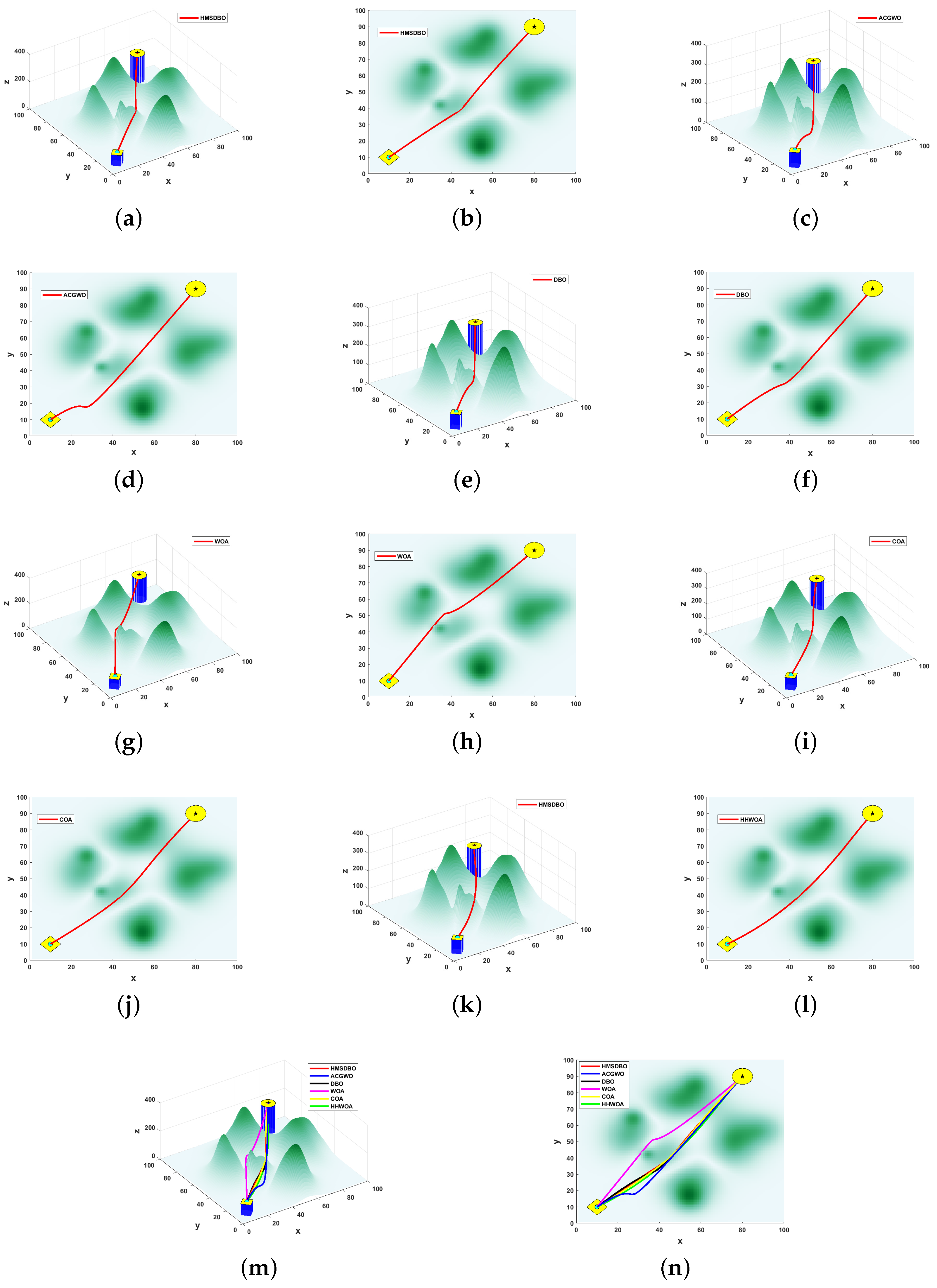
5.2. Testing of Path Planning Algorithms for Agricultural UAV

To assess the performance of the HMSDBO algorithm, several functions from the CEC-2005 test set were selected for evaluation, as detailed in Table 4. Each algorithm was executed 30 times, and the average values were recorded. The population size for all algorithms was set to 30, and each was run for 200 iterations. Table 5 provides a comparative analysis of the performance outcomes of six algorithms—HMSDBO, ACGWO, DBO, WOA, COA, and HHWOA—across various test functions.
As illustrated in the figure, the performance of the algorithms across several test functions (F1 to F9) varies significantly. Notably, HMSDBO demonstrates strong optimization capabilities for most test functions. In functions such as F1, F4, F5, and F6, HMSDBO converges significantly faster than other algorithms, with fitness values decreasing rapidly and stabilizing after fewer iterations. This indicates its superior global search ability and high local convergence accuracy. For more complex functions like F2, F3, and F9, HMSDBO also exhibits a significant performance advantage. While its rate of decline in the initial stages is slightly slower, it quickly converges to the optimal solution during later iterations.
Table 6 shows that HMSDBO performs competitively across nine test functions, using minimum, mean, and standard deviation as evaluation metrics. It achieves better accuracy and stability, particularly on F1, F4, F5, and F9, demonstrating strong robustness compared to other algorithms.
Table 7 presents the results of the Wilcoxon rank-sum test conducted to assess the statistical significance of performance differences between HMSDBO and the comparative algorithms across nine benchmark functions (F1–F9). As shown, HMSDBO achieves highly significant improvements in the majority of cases. Specifically, for functions F1, F3, F5, F6, and F8, the p-values between HMSDBO and other algorithms are consistently below the conventional significance threshold of 0.05, indicating that the performance enhancements are statistically significant. For instance, HMSDBO significantly outperforms DBO and COA on F1 with a p-value of 3.0199 × 10⁻¹¹, and demonstrates superiority on F4 with a p-value of 3.9881 × 10⁻⁴. Notably, even in functions such as F2 and F7, where p-values between HMSDBO and some baselines reach 1.0000, this suggests comparable performances rather than degradation. These results collectively validate the robustness and competitiveness of HMSDBO, as its performance gains are not only consistent but also statistically reliable across diverse test cases.
In contrast, HHWOA shows a weaker performance compared to HMSDBO on most test functions, particularly F4 and F9. As illustrated in Figure 3, While HHWOA achieves a rapid decrease in fitness values during early iterations, its improvement potential becomes limited in later iterations, resulting in less favorable final convergence outcomes compared to HMSDBO. WOA and COA demonstrate moderate performance across several functions. Although they are initially comparable to HMSDBO during early iterations, they quickly converge and reach optimal solutions later. However, as iterations progress, their fitness value improvements slow down, making it challenging for them to match HMSDBO’s optimization performance.
Of particular note is the weak performance of ACGWO, especially on functions such as F1, F3, F4, and F9. For these functions, the fitness values of ACGWO show minimal change and even stagnate early, indicating premature convergence that prevents it from exploring a broader search space or achieving more optimal solutions.
Overall, HMSDBO exhibits exceptional performance in path planning problems. It demonstrates strong exploration capabilities during the global search phase to quickly identify potential optimal solutions and excels in refining these solutions during the local search phase, ultimately achieving optimal convergence. By comparison, although the other algorithms possess certain convergence capabilities, their performance and efficiency in tackling complex problems fall short of HMSDBO’s. This is especially evident in large−scale problems or multi−objective optimization tasks, where HMSDBO’s advantages are more pronounced. These findings highlight HMSDBO’s robustness and generalizability, making it well suited for a variety of complex UAV path planning scenarios.

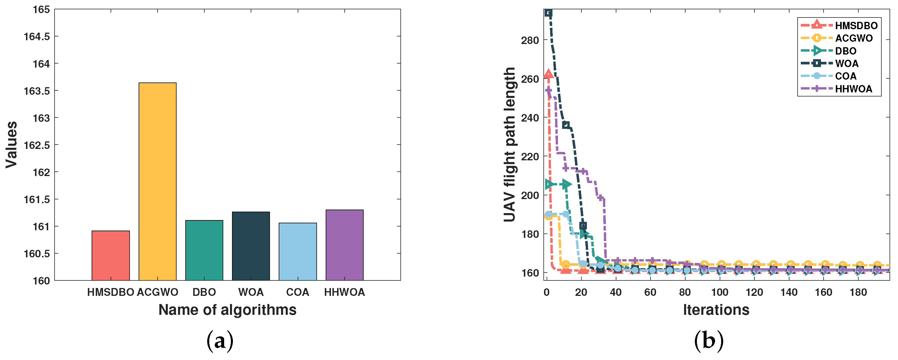
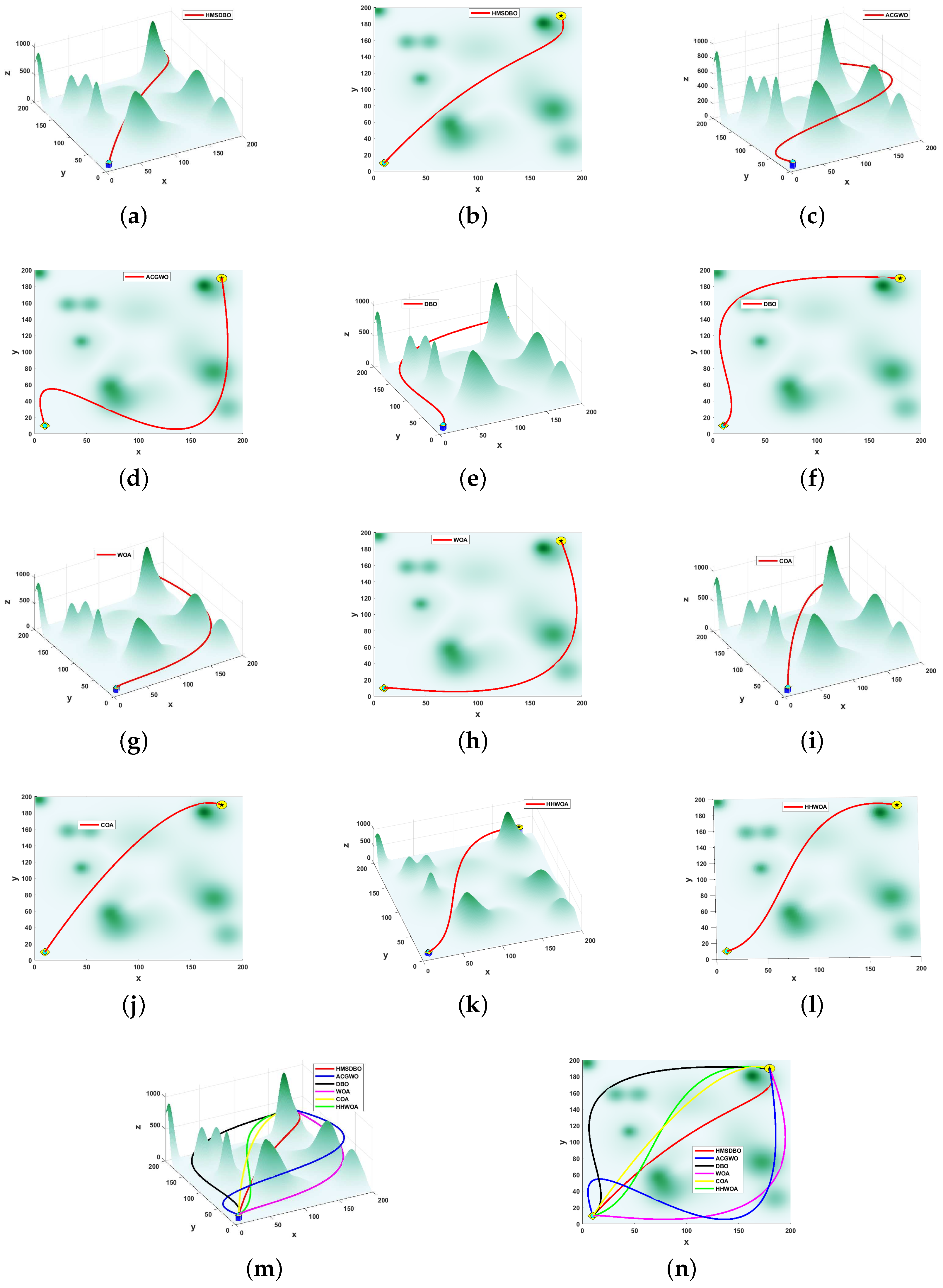
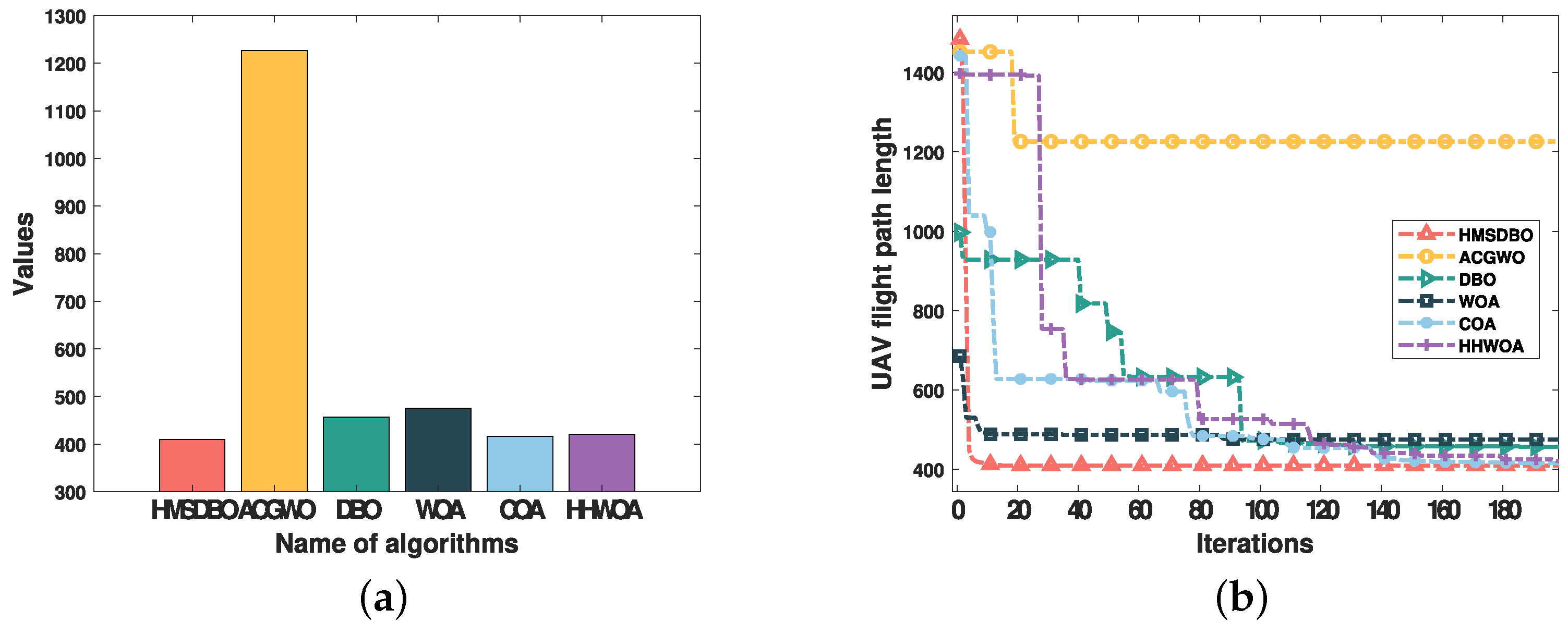
5.3. Simulation Results and Analysis

To thoroughly evaluate the effectiveness of the proposed algorithm, this study conducts a series of experimental tests to examine its convergence rate, optimization capabilities, and stability under various conditions. Additionally, comparative experiments with other evolutionary algorithms were performed to further validate the algorithm’s applicability and advantages in solving complex problems. During the experiments, all parameter settings were configured strictly in accordance with practical application requirements. Each algorithm was executed 50 times, and the average values were recorded to ensure the scientific rigor and reproducibility of the results. Figure 4 presents the simulation diagrams of various algorithms applied to Peak Model 1.
In this simulation experiment, the performance of multiple algorithms is compared for the complex environment of agricultural UAV path planning, and the simulation area is set as 100 × 100 × 400, containing five peaks. By comparing the path planning results of the six algorithms, HMSDBO, ACGWO, DBO, WOA, COA, and HHWOA, it can be observed that HMSDBO performs well in terms of optimal path value, path smoothness, and convergence speed.
As illustrated in Figure 4, HMSDBO demonstrates outstanding performance in path planning from both horizontal and top–down viewpoints. Specifically, HMSDBO not only successfully avoids all obstacles but also achieves a high level of path smoothness, producing results closer to the optimal solution compared to other algorithms. While ACGWO, DBO, WOA, COA, and HHWOA also completed the path planning tasks, their performance fell short of HMSDBO in terms of path smoothness and overall obstacle avoidance. In three-dimensional space, the paths generated by HMSDBO had the shortest total distances, highlighting its superior optimization capability when addressing a multi-peaked complex terrain.
Figure 5a illustrates the minimum path length plots. Further numerical analysis reveal that the optimal path value of HMSDBO is 160.914, which is significantly lower than the values achieved by the other algorithms: 163.64 for ACGWO, 161.103 for DBO, 161.261 for WOA, 161.058 for COA, and 161.298 for HHWOA. These results indicate that HMSDBO performs optimally in this experiment. The smaller the optimal value, the better the algorithm performs in terms of optimization metrics such as energy consumption and time, particularly in complex path planning scenarios. By comparing the optimal values, HMSDBO outperforms ACGWO by 1.67%, DBO by 0.12%, WOA by 0.21%, COA by 0.09%, and HHWOA by 0.24%. Although the improvements over some algorithms are relatively small, HMSDBO consistently achieves the global optimal solution, demonstrating the superiority of the proposed algorithm.
In addition, the convergence curve shows that HMSDBO achieves a significantly faster convergence rate compared to the other algorithms. Figure 5b illustrates the convergence process of each algorithm, where HMSDBO rapidly converges within fewer iterations, demonstrating its strong global search capability and high convergence efficiency in finding the optimal path. In contrast, other algorithms, such as ACGWO and DBO, require more iterations to approach the optimal value, highlighting their disadvantage in convergence speed.
The simulation of Scenario 2 is presented in Figure 6, which features a simulation area of 200 × 200 × 1000 containing 10 peaks. Figure 6 depicts the path planning results of these algorithms in a complex environment and evaluates them from various perspectives to provide a comprehensive assessment of their strengths and weaknesses.
First, from the perspective of path planning performance, the HMSDBO algorithm demonstrates clear advantages in planning paths. In both the horizontal view (a) and top–down view (b), HMSDBO successfully avoids all obstacles while following the shortest and smoothest path, highlighting its excellent global search and path optimization capabilities in complex terrains. In contrast, ACGWO generates significantly longer paths, indicating its poor performance in this simulation task and its inability to find an optimal path. Meanwhile, DBO, WOA, COA, and HHWOA also complete the path planning task, but their path lengths are longer than that of HMSDBO, revealing varying degrees of sub-optimal performance.
From the numerical results, the optimal path value of HMSDBO is 409.897, which is notably lower than the values produced by the other algorithms. Specifically, the best path value of ACGWO is 1226.2, significantly higher than that of other algorithms, further demonstrating its ineffectiveness in a complex terrain. The optimal path values of the other algorithms are as follows: 456.981 for DBO, 475.416 for WOA, 416.386 for COA, and 420.386 for HHWOA. HMSDBO achieved the shortest path length, underscoring its superior path planning performance.
Figure 7a illustrates the minimum path length plots. Further performance analysis reveals that HMSDBO outperforms ACGWO by 67.6%, DBO by 10.3%, WOA by 13.8%, COA by 1.56%, and HHWOA by 2.48%. These results confirm that HMSDBO achieves the best performance in this UAV path planning task, particularly when compared to ACGWO, where the path length was reduced by more than 67%. Although HMSDBO shows relatively smaller improvements compared to some other algorithms, it consistently achieves the best results in global path planning.
From the convergence curve in Figure 7b, HMSDBO exhibits a faster convergence speed during the iteration process, reaching a stable optimal solution earlier. This further validates its strong global search capability and efficient convergence. In contrast, algorithms such as ACGWO and WOA demonstrate slower convergence speeds and exhibit large fluctuations during the iteration process, indicating instability in their path optimization processes and a tendency to fall into local optima.
In Scenario 3, the simulation area is 300 × 300 × 1500 and includes 20 peaks. The performance of different algorithms in a complex 3D terrain is shown in Figure 8. Among all tested algorithms, the HMSDBO algorithm demonstrates the best path planning capability, achieving an optimal value of 660.625. This result is significantly better than those of ACGWO, DBO, WOA, COA, and HHWOA. Specifically, HMSDBO reduces the path length by 26.91% compared to ACGWO, 3.19% compared to DBO, 30.53% compared to WOA, and 6.68% and 6.36% compared to COA and HHWOA, respectively.
Figure 9a illustrates the convergence graphs of the six algorithms. From the figure, it is evident that HMSDBO exhibits a fast and stable convergence trend, outperforming other algorithms with faster convergence and reduced volatility. This result highlights HMSDBO’s significant advantage in global search capability in complex terrains, effectively avoiding local optimization problems while maintaining a smooth path. Overall, HMSDBO surpasses other similar algorithms in both path optimization and convergence speed, underscoring its strong potential for agricultural UAV path planning.
In Scenario 4, the simulation area is 500 × 500 × 4000 and contains 30 peaks. The results of various algorithms are depicted in Figure 10 and Figure 11. Among all tested algorithms, the HMSDBO algorithm performs optimally in this test, achieving an optimal path value of 1227.75. This result is significantly better than those of ACGWO, DBO, WOA, COA, and HHWOA. Specifically, HMSDBO reduces the path length by 14.44% compared to ACGWO, 17.9% compared to DBO, 35.25% compared to WOA, 24.01% compared to COA, and 7.71% compared to HHWOA.
The convergence of HMSDBO also shows a significant advantage, as evidenced by the convergence curve in Figure 11b. The algorithm converges rapidly in the early search phase and exhibits a stable downward trend throughout the optimization process, effectively avoiding the problem of local optimality often encountered by other algorithms. Compared with the other methods, HMSDBO demonstrates superior global search capability and path optimization performance when solving the agricultural UAV path planning problem in complex 3D terrains. These findings suggest that HMSDBO offers considerable benefits in terms of both the shortest path length and the quickest convergence speed, making it well suited for agricultural UAV path planning in challenging environments.
As observed across Scenarios 1 to 4, the paths planned by HMSDBO consistently outperform those of other algorithms in terms of path length, obstacle avoidance, and computational efficiency, even as the complexity of the environment model and flight area increases. This highlights the algorithm’s robustness and adaptability in handling complex environments, maintaining strong global optimization capability in large search spaces, and generating more efficient path solutions.
Figure 12a–d illustrate the adaptation values over 100 runs for each scenario. In Scenario 1, HMSDBO achieves the lowest adaptation value, reflecting its superior optimization performance in minimizing combined costs such as total flight distance, obstacle avoidance, and compliance with specified boundaries. Despite some fluctuations, HMSDBO maintains a low overall adaptation value, underscoring its stability in this scenario. In contrast, other algorithms, such as ACGWO, DBO, and COA, exhibit higher adaptation values, with ACGWO showing particularly high costs, demonstrating its inferior performance compared to HMSDBO.
In Scenario 2, HMSDBO achieves adaptation values ranging from 450 to 500, maintaining the lowest values among all tested algorithms. This demonstrates its effectiveness in optimizing UAV flight costs for this scenario. Conversely, ACGWO exhibits adaptation values between approximately 700 and 850, indicating significantly higher flight costs and a failure to effectively manage obstacle avoidance and boundary control, leading to suboptimal performance relative to HMSDBO.
In Scenario 3, HMSDBO again maintains the lowest adaptation values, ranging from 650 to 750, demonstrating its ability to effectively minimize flight costs. In comparison, ACGWO and DBO have adaptation values between 800 and 950, reflecting higher flight costs and less effective optimization. Similarly, in Scenario 4, HMSDBO registers the lowest adaptation values, ranging from 1200 to 1300, confirming its strong performance in controlling flight costs in complex environments. By contrast, ACGWO exhibits significantly higher adaptation values, ranging from 1800 to 2000, highlighting its greater flight costs and inadequate optimization for obstacle avoidance and path planning.
Across all four scenarios, HMSDBO consistently demonstrates the lowest flight costs, showcasing significant optimization in reducing total UAV flight distances, obstacle avoidance costs, and boundary control penalties. In contrast, ACGWO and other algorithms typically exhibit higher flight costs, particularly in more complex scenarios. These results reinforce that HMSDBO delivers an optimal overall performance in UAV path planning, effectively reducing flight costs and enhancing operational efficiency.

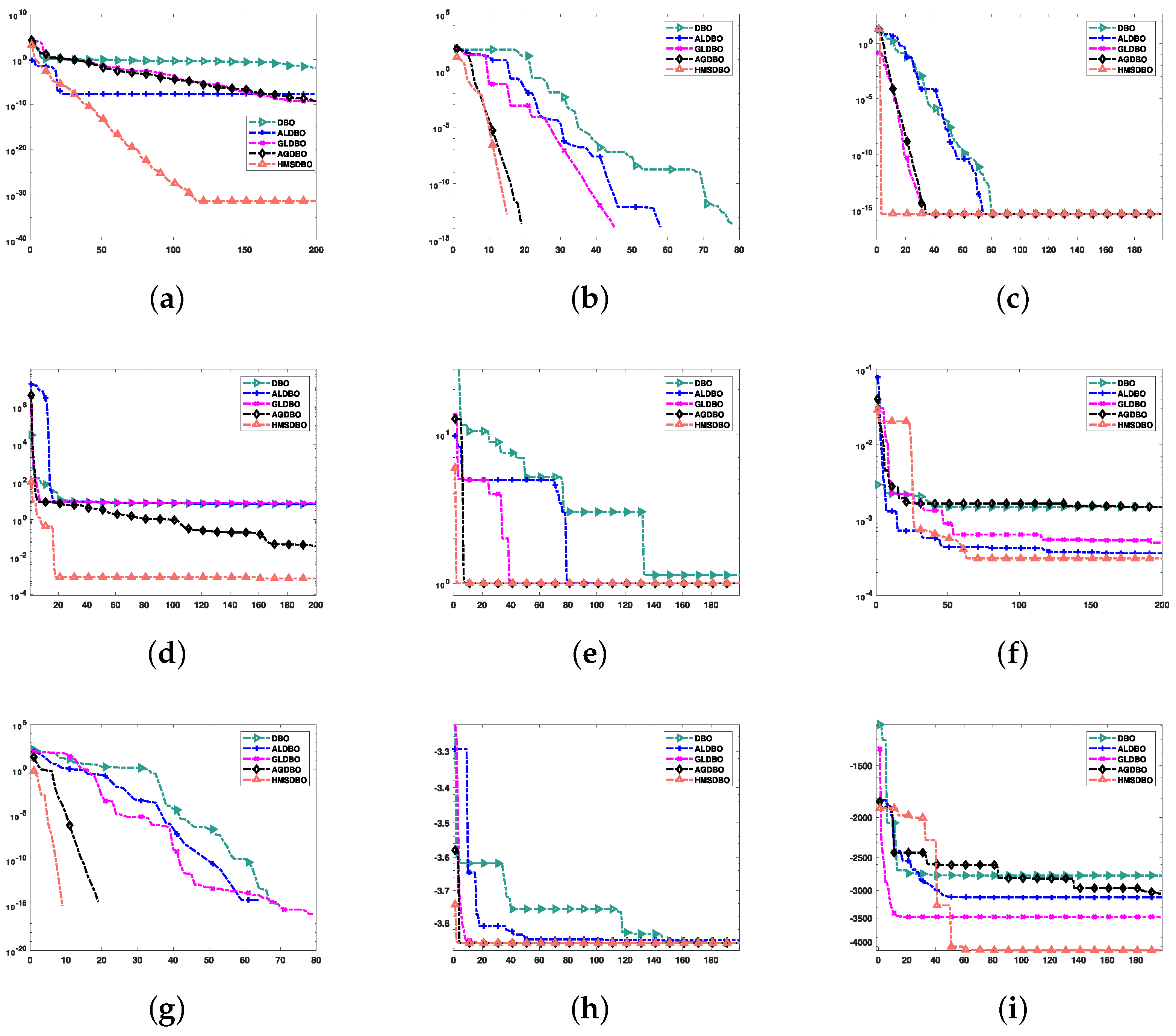
5.4. Ablation Experiments

To further validate the advantages of the HMSDBO proposed in this paper for 3D path planning in agricultural UAVs, a series of ablation experiments were conducted. Specifically, the impact of each key strategy within the HMSDBO algorithm on path planning performance was analyzed by progressively removing these strategies. First, the Latin hypercube sampling strategy was removed to evaluate its role in enhancing population diversity and global search capability, resulting in a variant named AGDBO. Next, the golden sine strategy was independently removed to assess its contribution to improving the algorithm’s robustness, forming the variant ALDBO. Then, the hybrid adaptive weighting strategy was excluded to test its effect on the stability and reliability of the algorithm, producing the variant GLDBO. To compare the performance differences among the five algorithms—HMSDBO, AGDBO, ALDBO, GLDBO, and DBO—a set of functions from the CEC-2005 test suite (as presented in Table 5) was utilized. These tests primarily examined the algorithms’ performance in terms of path length, convergence speed, stability, and robustness. The results of the tests are illustrated in Figure 13.
The experimental results demonstrate that HMSDBO exhibits superior performance across various types of functions. For single-peak functions (F1, F4, F6), HMSDBO showcases rapid convergence and exceptional accuracy, particularly on F1, where its global search ability enables it to quickly approach the optimal value. In contrast, AGDBO, after removing the Latin Hypercube Sampling Strategy, suffers from a significant loss in accuracy due to reduced population diversity. For multi-peak functions (F2, F3, F5, F7), HMSDBO’s advantage is even more pronounced. The incorporation of the golden sine strategy allows the algorithm to achieve a dynamic balance between global exploration and local exploitation, enabling it to escape local optima in complex search spaces effectively. Consequently, HMSDBO achieves substantially better error values on F2 and F3 compared to other algorithms, while ALDBO, without the golden sine strategy, experiences a marked decline in search ability and delivers inferior results. On discrete and discontinuous functions (F8, F9), HMSDBO demonstrates robust performance and stability through its hybrid adaptive weighting strategy, producing smooth convergence curves and the highest final solution accuracy. In contrast, GLDBO exhibits greater instability without this strategy, particularly on F8, where it struggles to converge to an optimal solution. Additionally, the benchmark DBO algorithm shows clear deficiencies across all test functions, underperforming significantly in both convergence speed and final accuracy compared to other algorithms. Based on the experimental results and the properties of the CEC-2005 test functions, HMSDBO demonstrates outstanding convergence on single-peak functions, strong capability to escape local optima on multi-peak functions, and high robustness in discrete and discontinuous problems. These results confirm that HMSDBO achieves an effective integration of global exploration, local exploitation, and algorithmic stability through the introduction of key strategies, providing a reliable foundation for efficiently solving UAV 3D path planning problems.
By analyzing the UAV path planning and ablation experiment results shown in Figure 14, the advantages of the HMSDBO algorithm in 3D path planning are clearly evident. The experiments evaluated five algorithms (HMSDBO, ALDBO, AGDBO, GLDBO, and DBO) in terms of path visualization, path length comparison, and convergence performance, and confirmed the contributions of individual strategies to algorithm performance.
From the 3D and 2D path visualizations (Figure 14a,b), it is evident that the path generated by HMSDBO (red curve) outperforms all other algorithms. Its path is not only the shortest and smoothest but also effectively avoids obstacles in complex terrains. In comparison, the paths generated by DBO and AGDBO (green and blue curves, respectively) are significantly longer with unnecessary detours, indicating their limited global search capabilities and inability to effectively optimize paths. GLDBO (pink curve) generates smoother paths but introduces excessively large detours, making its results suboptimal. Meanwhile, ALDBO (black curve) produces paths close to those of HMSDBO but slightly less optimal, maintaining commendable performance in diverse path searches. These observations highlight HMSDBO’s ability to balance global and local optimization effectively, thanks to mechanisms such as hybrid adaptive weights and the golden sine strategy.
The comparative path length results are visualized in the histogram (Figure 14c). HMSDBO achieves the shortest path length, significantly outperforming other algorithms, further validating its superiority in UAV path planning. Conversely, GLDBO records the longest path length, indicating that the removal of the hybrid adaptive weighting strategy substantially hampers its performance, disrupting the balance between exploration and exploitation. The path lengths of ALDBO and AGDBO are slightly higher than that of HMSDBO, emphasizing the critical roles of the golden sine strategy and the Latin Hypercube Sampling strategy in enhancing performance. The original DBO algorithm, with the longest path lengths, performs the worst, underscoring the significant improvements introduced by HMSDBO.
HMSDBO’s advantages in convergence speed and stability are further evidenced by the convergence performance graph (Figure 14d). Throughout the iterations, HMSDBO’s convergence curve declines the fastest and stabilizes after approximately 100 iterations, ultimately achieving the shortest path length. This indicates an efficient and stable optimization process. In contrast, the convergence curves of GLDBO and AGDBO decline more slowly and stagnate during later optimization stages, failing to achieve optimal path lengths. This reflects their limitations in escaping local optima and achieving convergence accuracy. DBO has the slowest convergence speed, highlighting its lack of global search ability. ALDBO, while not as fast as HMSDBO in early iterations, converges to near-optimal results in the end, demonstrating the importance of the golden sine strategy in enhancing global exploration capability.
In conclusion, the comprehensive analysis of 3D path planning, path length, and convergence curves reveals that HMSDBO, through the integration of the Latin Hypercube Sampling strategy, the golden sine strategy, and the hybrid adaptive weighting strategy, successfully combines global exploration, local exploitation, and algorithm stability. This enables HMSDBO to generate optimal paths in UAV path planning problems and significantly outperform both its algorithmic variants and the original DBO algorithm. These experimental results verify HMSDBO’s superior performance and practical value in UAV path planning tasks.

5.5. Discussion

This section provides an interpretation of the experimental results presented in Section 5.2, with a focus on the performance of the HMSDBO algorithm in agricultural UAV path planning.
(1)
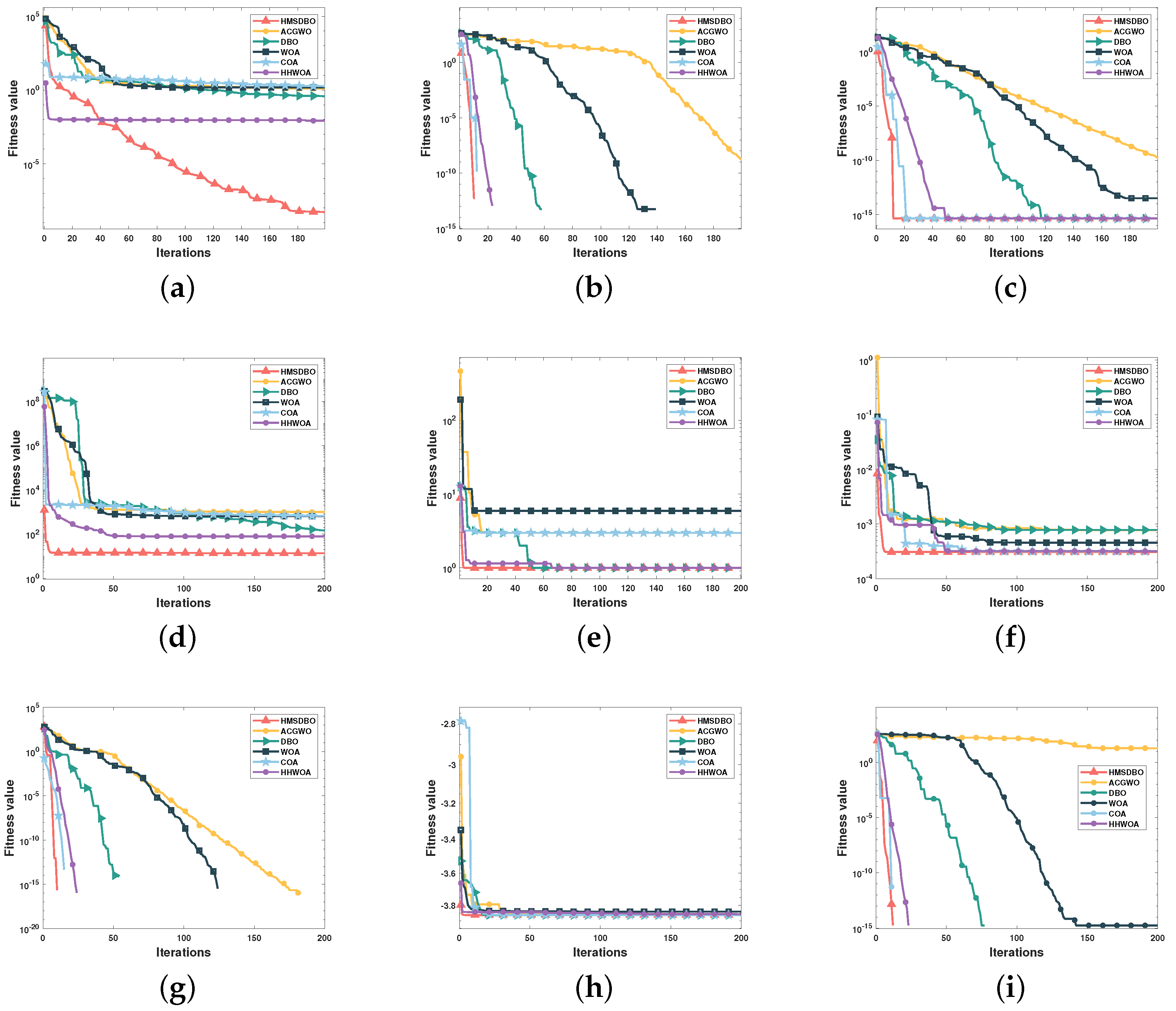
Algorithm Performance: The HMSDBO algorithm outperforms several benchmark algorithms, including ACGWO, DBO, WOA, COA, and HHWOA, in terms of both path length reduction and path smoothness. The integration of hybrid strategies, such as Latin Hypercube Sampling (LHS) and Hybrid Adaptive Weighting, contributes to the improved exploration and exploitation capabilities of HMSDBO.
(2)
Convergence Rate: HMSDBO exhibited faster convergence compared to the other algorithms. This efficiency is due to the algorithm’s ability to balance global search and local refinement, allowing it to quickly find high-quality solutions while maintaining stability.
(3)
Real-World Relevance: The improvements in path length and smoothness demonstrate HMSDBO’s potential for real-world applications, especially in UAV operations, where efficient path planning is crucial. The algorithm’s ability to adapt to obstacles and dynamic environments further supports its applicability in agricultural UAVs.
(4)
Limitations and Future Work: Despite promising results, HMSDBO’s performance could be improved in highly dynamic environments, such as real-time path replanning scenarios. Future research could focus on enhancing HMSDBO’s scalability and robustness, particularly in large-scale UAV systems and complex real-world conditions.

6. Conclusions

This paper proposes a novel 3D path planning method for agricultural unmanned aerial vehicles (UAVs) based on the Hybrid Multi-Strategy Dung Beetle Optimization Algorithm (HMSDBO), which significantly enhances the efficiency and accuracy of path searches. The effectiveness of HMSDBO is validated through a series of experimental comparisons with other algorithms, including the Adaptive Chaotic Gray Wolf Optimization Algorithm (ACGWO), Primitive Dung Beetle Optimization Algorithm (DBO), Whale Optimization Algorithm (WOA), Crayfish Optimization Algorithm (COA), and Hyper-Heuristic Whale Optimization Algorithm (HHWOA).
Quantitative experimental results demonstrate the superior performance of HMSDBO in optimizing 3D path planning for agricultural UAVs. Specifically, compared to ACGWO, HMSDBO achieves a 21.3% reduction in path length; compared to DBO, the reduction is 7.88%; compared to WOA, it achieves a 19.95% reduction; compared to COA, the reduction is 8.09%; and compared to HHWOA, the path length is reduced by 4.2%. These results clearly show that HMSDBO not only reduces path length but also significantly improves both path smoothness and the overall optimization effectiveness.
Moreover, HMSDBO demonstrates faster convergence and stronger global search capabilities. In particular, in complex agricultural environments, HMSDBO achieves optimal solutions in fewer iterations, showcasing its superior global exploration ability and high local convergence accuracy.
These results substantiate the effectiveness of HMSDBO in UAV path planning, especially in dynamic and high-dimensional agricultural environments. It offers significant potential for enhancing the efficiency and safety of UAV operations. Future work will focus on further improving HMSDBO’s scalability and adaptability for real-time path re-planning and large-scale applications, expanding its potential use in agricultural UAV operations and other real-time optimization contexts.

Author Contributions

All authors contributed to the study’s conception and design. H.F. and J.Z.: Conceptualization, investigation, writing and modification. R.L. and L.D.: Writing, conceptualization, review, and editing. Z.D.: Supervision. X.L.: Methodology. T.L.: Investigation. The first draft of the manuscript was written by H.F. and all authors commented on previous versions of the manuscript. All authors have read and agreed to the published version of the manuscript.

Funding

This paper was funded by the project of the National Key Research and Development Program of the Corps: Research and application demonstration of information technology based on source-grid-load-storage and multi-energy complementarity, grant number: 2023AB021; National Key Research and Development Program of the Corps: Key Technology Research and Application for High Penetration New Energy Grid Dispatch, grant number: 2023AB010; National Key Research and Development Program of the Corps: R&D and the demonstration of the intelligent supervision platform for the inspection and testing institutions of the Corps based on big data and artificial intelligence, grant number: 2024AB063; Young scientific and technological innovation talents: key technological innovation and application of integrated energy intelligent management and control and precise low-carbon dispatching, grant number: 2023TSYCCx0120; Corps Science and Technology Program Project-Corps Regional Innovation Guidance Program, grant number: 2023ZD045.

Data Availability Statement

The data that support the findings of this study are available from the corresponding author.

Conflicts of Interest

The authors declare no competing interests.

References

  1. Chen, C.; Zheng, Z.; Xu, T.; Guo, S.; Feng, S.; Yao, W.; Lan, Y. Yolo-based uav technology: A review of the research and its applications. Drones 2023, 7, 190. [Google Scholar] [CrossRef]
  2. Samad, A.M.; Kamarulzaman, N.; Hamdani, M.A.; Mastor, T.A.; Hashim, K.A. The potential of Unmanned Aerial Vehicle (UAV) for civilian and mapping application. In Proceedings of the 2013 IEEE 3rd International Conference on System Engineering and Technology, Shah Alam, Malaysia, 19–20 August 2013; IEEE: New York, NY, USA, 2013; pp. 313–318. [Google Scholar]
  3. Cienciała, A.; Sobura, S.; Sobolewska-Mikulska, K. Optimising land consolidation by implementing UAV technology. Sustainability 2022, 14, 4412. [Google Scholar] [CrossRef]
  4. Sishodia, R.P.; Ray, R.L.; Singh, S.K. Applications of remote sensing in precision agriculture: A review. Remote Sens. 2020, 12, 3136. [Google Scholar] [CrossRef]
  5. Chamas, M.H.; Amine, S.; Gazo Hanna, E.; Mokhiamar, O. Control of a novel parallel mechanism for the stabilization of unmanned aerial vehicles. Appl. Sci. 2023, 13, 8740. [Google Scholar] [CrossRef]
  6. Latifinavid, M.; Azizi, A. Kinematic modelling and position control of a 3-DOF parallel stabilizing robot manipulator. J. Intell. Robot. Syst. 2023, 107, 17. [Google Scholar] [CrossRef]
  7. Chamas, M.H.; Amine, S.; Gazo-Hanna, E.; El Gohary, M. AI-Driven Kinematics and Experimental Control of 3-SRR Mechanism for UAV Stabilization. Results Eng. 2025, 26, 105131. [Google Scholar] [CrossRef]
  8. Aggarwal, S.; Kumar, N. Path planning techniques for unmanned aerial vehicles: A review, solutions, and challenges. Comput. Commun. 2020, 149, 270–299. [Google Scholar] [CrossRef]
  9. Ait Saadi, A.; Soukane, A.; Meraihi, Y.; Benmessaoud Gabis, A.; Mirjalili, S.; Ramdane-Cherif, A. UAV path planning using optimization approaches: A survey. Arch. Comput. Methods Eng. 2022, 29, 4233–4284. [Google Scholar] [CrossRef]
  10. Müller, H.; Niculescu, V.; Polonelli, T.; Magno, M.; Benini, L. Robust and efficient depth-based obstacle avoidance for autonomous miniaturized uavs. IEEE Trans. Robot. 2023, 39, 4935–4951. [Google Scholar] [CrossRef]
  11. Wang, L.; Lan, Y.; Zhang, Y.; Zhang, H.; Tahir, M.N.; Ou, S.; Liu, X.; Chen, P. Applications and prospects of agricultural unmanned aerial vehicle obstacle avoidance technology in China. Sensors 2019, 19, 642. [Google Scholar] [CrossRef]
  12. Froese, V.; Hertrich, C. Training neural networks is NP-hard in fixed dimension. Adv. Neural Inf. Process. Syst. 2023, 36, 44039–44049. [Google Scholar]
  13. Dudeja, C.; Kumar, P. An improved weighted sum-fuzzy Dijkstra’s algorithm for shortest path problem (iWSFDA). Soft Comput. 2022, 26, 3217–3226. [Google Scholar] [CrossRef]
  14. Li, B.; Chen, B. An adaptive rapidly-exploring random tree. IEEE/CAA J. Autom. Sin. 2021, 9, 283–294. [Google Scholar] [CrossRef]
  15. Goel, L. An extensive review of computational intelligence-based optimization algorithms: Trends and applications. Soft Comput. 2020, 24, 16519–16549. [Google Scholar] [CrossRef]
  16. Tang, J.; Liu, G.; Pan, Q. A review on representative swarm intelligence algorithms for solving optimization problems: Applications and trends. IEEE/CAA J. Autom. Sin. 2021, 8, 1627–1643. [Google Scholar] [CrossRef]
  17. Liu, R.; Mo, Y.; Lu, Y.; Lyu, Y.; Zhang, Y.; Guo, H. Swarm-intelligence optimization method for dynamic optimization problem. Mathematics 2022, 10, 1803. [Google Scholar] [CrossRef]
  18. Ramírez-Ochoa, D.D.; Pérez-Domínguez, L.A.; Martínez-Gómez, E.A.; Luviano-Cruz, D. PSO, a swarm intelligence-based evolutionary algorithm as a decision-making strategy: A review. Symmetry 2022, 14, 455. [Google Scholar] [CrossRef]
  19. Xue, J.; Shen, B. Dung beetle optimizer: A new meta-heuristic algorithm for global optimization. J. Supercomput. 2023, 79, 7305–7336. [Google Scholar] [CrossRef]
  20. Ye, M.; Zhou, H.; Yang, H.; Hu, B.; Wang, X. Multi-strategy improved dung beetle optimization algorithm and its applications. Biomimetics 2024, 9, 291. [Google Scholar] [CrossRef]
  21. Huang, Q.; Sun, Y.; Kang, C.; Fan, C.; Liang, X.; Sun, F. An Improved Crayfish Optimization Algorithm: Enhanced Search Efficiency and Application to UAV Path Planning. Symmetry 2025, 17, 356. [Google Scholar] [CrossRef]
  22. Rana, N.; Latiff, M.S.A.; Abdulhamid, S.M.; Chiroma, H. Whale optimization algorithm: A systematic review of contemporary applications, modifications and developments. Neural Comput. Appl. 2020, 32, 16245–16277. [Google Scholar] [CrossRef]
  23. Zhang, N.; Zhang, M.; Low, K.H. 3D path planning and real-time collision resolution of multirotor drone operations in complex urban low-altitude airspace. Transp. Res. Part C Emerg. Technol. 2021, 129, 103123. [Google Scholar] [CrossRef]
  24. Chen, J.; Li, M.; Yuan, Z.; Gu, Q. An improved A* algorithm for UAV path planning problems. In Proceedings of the 2020 IEEE 4th Information Technology, Networking, Electronic and Automation Control Conference (ITNEC), Chongqing, China, 12–14 June 2020; IEEE: New York, NY, USA, 2020; Volume 1, pp. 958–962. [Google Scholar]
  25. Bai, X.; Jiang, H.; Cui, J.; Lu, K.; Chen, P.; Zhang, M. UAV path planning based on improved A* and DWA algorithms. Int. J. Aerosp. Eng. 2021, 2021, 4511252. [Google Scholar] [CrossRef]
  26. Mandloi, D.; Arya, R.; Verma, A.K. Unmanned aerial vehicle path planning based on A* algorithm and its variants in 3D environment. Int. J. Syst. Assur. Eng. Manag. 2021, 12, 990–1000. [Google Scholar] [CrossRef]
  27. Dhulkefl, E.; Durdu, A.; Terzioğlu, H. Dijkstra algorithm using UAV path planning. Konya J. Eng. Sci. 2020, 8, 92–105. [Google Scholar] [CrossRef]
  28. Guo, J.; Xia, W.; Hu, X.; Ma, H. Feedback RRT* algorithm for UAV path planning in a hostile environment. Comput. Ind. Eng. 2022, 174, 108771. [Google Scholar] [CrossRef]
  29. Fan, J.; Chen, X.; Wang, Y.; Chen, X. UAV trajectory planning in cluttered environments based on PF-RRT* algorithm with goal-biased strategy. Eng. Appl. Artif. Intell. 2022, 114, 105182. [Google Scholar] [CrossRef]
  30. Avcu, M.E.; Gökçe, H.; Şahin, İ. A WOA-based path planning approach for UAVs to avoid collisions in cluttered areas. In Handbook of Whale Optimization Algorithm; Elsevier: Amsterdam, The Netherlands, 2024; pp. 449–461. [Google Scholar]
  31. Yu, B.; Fan, S.; Cui, W.; Xia, K.; Wang, L. A Multi-UAV cooperative mission planning method based on SA-WOA algorithm for three-dimensional space atmospheric environment detection. Robotica 2024, 42, 1–38. [Google Scholar] [CrossRef]
  32. Liu, X.; Li, G.; Yang, H.; Zhang, N.; Wang, L.; Shao, P. Agricultural UAV trajectory planning by incorporating multi-mechanism improved grey wolf optimization algorithm. Expert Syst. Appl. 2023, 233, 120946. [Google Scholar] [CrossRef]
  33. Zhang, W.; Zhang, S.; Wu, F.; Wang, Y. Path planning of UAV based on improved adaptive grey wolf optimization algorithm. IEEE Access 2021, 9, 89400–89411. [Google Scholar] [CrossRef]
  34. Shen, Q.; Zhang, D.; Xie, M.; He, Q. Multi-strategy enhanced dung beetle optimizer and its application in three-dimensional UAV path planning. Symmetry 2023, 15, 1432. [Google Scholar] [CrossRef]
  35. Lyu, L.; Jiang, H.; Yang, F. Improved Dung Beetle Optimizer Algorithm with Multi-Strategy for global optimization and UAV 3D path planning. IEEE Access 2024, 12, 69240–69257. [Google Scholar] [CrossRef]
  36. Li, F.F.; Du, Y.; Jia, K.J. Path planning and smoothing of mobile robot based on improved artificial fish swarm algorithm. Sci. Rep. 2022, 12, 659. [Google Scholar] [CrossRef] [PubMed]
  37. Tripicchio, P.; Unetti, M.; D’Avella, S.; Avizzano, C.A. Smooth coverage path planning for UAVs with model predictive control trajectory tracking. Electronics 2023, 12, 2310. [Google Scholar] [CrossRef]
  38. Liu, Z.; Wen, S.; Huang, G.; Li, S.; Deng, Z. Agricultural UAV obstacle avoidance system based on a depth image inverse projection algorithm and B-spline curve trajectory optimization algorithm. Inf. Technol. Control 2024, 53, 736–757. [Google Scholar]
  39. Liu, M.; Zhang, H.; Yang, J.; Zhang, T.; Zhang, C.; Bo, L. A path planning algorithm for three-dimensional collision avoidance based on potential field and B-spline boundary curve. Aerosp. Sci. Technol. 2024, 144, 108763. [Google Scholar] [CrossRef]
  40. Tanyildizi, E.; Demir, Y. Golden sine algorithm: A novel nature-inspired optimization algorithm. Adv. Electr. Comput. Eng. 2017, 17, 71–78. [Google Scholar] [CrossRef]
Figure 1. Comparison chart of four initialization methods across different metrics. (a) Latin Hypercube Sampling Dimension Distribution; (b) Lenticular Reverse Learning Dimension Distribution; (c) Random Initialization Dimension Distribution; (d) Original Sand Cat Algorithm Dimension Distribution; (e) Latin Hypercube Sampling Value Histogram; (f) Lenticular Reverse Learning Value Histogram; (g) Random Initialization Value Histogram; (h) Original Sand Cat Algorithm Value Histogram.
Agriculture 15 01156 g001
Figure 2. Algorithm flowchart of HMSDBO.
Agriculture 15 01156 g002
Figure 3. Convergence plot of the algorithm in 6 under the CEC2005 test function. (a) F1; (b) F2; (c) F3; (d) F4; (e) F5; (f) F6; (g) F7; (h) F8; (i) F9.
Agriculture 15 01156 g003
Figure 4. Comparison plot of UAV path planning for 6 algorithms in scenario 1 environment. (a) HMSDBO—horizontal; (b) HMSDBO—top; (c) ACGWO—horizontal; (d) ACGWO—top; (e) DBO—horizontal; (f) DBO—top; (g) WOA—horizontal; (h) WOA—top; (i) COA—horizontal; (j) COA—top; (k) HHWOA—horizontal; (l) HHWOA—top; (m) Overall path planning in 3D; (n) Overall path planning in 2D. Note: Circles represent initial positions; asterisks indicate target positions.
Agriculture 15 01156 g004
Figure 5. Comparison of the convergence plots of the 6 algorithms in Scenario 1. (a) Path length bar graph; and (b) Convergence diagram.
Agriculture 15 01156 g005
Figure 6. Comparison plot of UAV path planning for 6 algorithms in scenario 2 environment. (a) HMSDBO—horizontal; (b) HMSDBO—top; (c) ACGWO—horizontal; (d) ACGWO—top; (e) DBO—horizontal; (f) DBO—top; (g) WOA—horizontal; (h) WOA—top; (i) COA—horizontal; (j) COA—top; (k) HHWOA—horizontal; (l) HHWOA—top; (m) Overall path planning in 3D; (n) Overall path planning in 2D. Note: Circles represent initial positions; asterisks indicate target positions.
Agriculture 15 01156 g006
Figure 7. Comparison of the convergence plots of the 6 algorithms in Scenario 2. (a) Path Length Bar Graph. (b) Convergence diagram.
Agriculture 15 01156 g007
Figure 8. Comparison plot of UAV path planning for 6 algorithms in scenario 3 environment. (a) HMSDBO—horizontal; (b) HMSDBO—top; (c) ACGWO—horizontal; (d) ACGWO—top; (e) DBO–horizontal; (f) DBO—top; (g) WOA—horizontal; (h) WOA—top; (i) COA—horizontal; (j) COA—top; (k) HHWOA—horizontal; (l) HHWOA—top; (m) Overall path planning in 3D; and (n) Overall path planning in 2D. Note: Circles represent initial positions; asterisks indicate target positions.
Agriculture 15 01156 g008
Figure 9. Comparison of the convergence plots of the 6 algorithms in Scenario 3. (a) Path length bar graph; (b) Convergence diagram.
Agriculture 15 01156 g009
Figure 10. Comparison plot of UAV path planning for 6 algorithms in Scenario 4 environment. (a) HMSDBO—horizontal; (b) HMSDBO—top; (c) ACGWO—horizontal; (d) ACGWO—top; (e) DBO—horizontal; (f) DBO—top; (g) WOA—horizontal; (h) WOA—top; (i) COA—horizontal; (j) COA—top; (k) HHWOA—horizontal; (l) HHWOA—top; (m) Overall path planning in 3D; (n) Overall path planning in 2D. Note: Circles represent initial positions; asterisks indicate target positions.
Agriculture 15 01156 g010
Figure 11. Comparison of the convergence plots of the 6 algorithms in Scenario 4. (a) Path length bar graph; (b) Convergence diagram.
Agriculture 15 01156 g011
Figure 12. Comparison of adaptation values after 100 repetitions in different scenes. (a) Scene 1; (b) Scene 2; (c) Scene 3; (d) Scene 4.
Agriculture 15 01156 g012
Figure 13. Convergence plot of the algorithm in 5 under the CEC2005 test function. (a) F1; (b) F2; (c) F3; (d) F4; (e) F5; (f) F6; (g) F7; (h) F8; and (i) F9.
Agriculture 15 01156 g013
Figure 14. Comparison of the adaptation values after 100 repetitions in different scenes. (a) Overall path planning in 3D; (b) Overall path planning in 2D; (c) Path length bar graph; (d) Convergence diagram. Note: Circles represent initial positions; asterisks indicate target positions.
Agriculture 15 01156 g014
Table 1. Parameters and their descriptions.
CharacterDescription
P s Path start
P e Path end
P i j The position of each dung beetle on the path
nThe number of dung beetles
P i The control points of the flight path
B i , k ( λ ) The basis function of the spline
hThe power of the B-spline function
( X i , Y i , Z i ) The coordinates of the control points
T c The total cost to bypass obstacles
V c The cost of flying within the specified boundaries
E c The total distance from start to end point
Table 2. Simulation Environment Parameters.
NameModel Number
CPUi7-7700HQ CPU @ 2.80 GHz
Random access memory32.0 GB
Operating systemWindows11
Programming languageMatlab
Test softwareMatlab R2021a
Table 3. Parameter settings for four simulation scenes.
Simulation Area (X, Y, Z)Start PointEnd PointNumber of Peaks
100 × 100 × 400 ( 10 , 10 , 80 ) ( 80 , 90 , 200 ) 5
200 × 200 × 1000 ( 10 , 10 , 80 ) ( 180 , 190 , 400 ) 10
300 × 300 × 1500 ( 10 , 10 , 80 ) 280 , 290 , 600 ) 20
500 × 500 × 4000 ( 10 , 10 , 80 ) ( 480 , 490 , 1000 ) 30
Table 4. Parameters for the comparative algorithms.
Algorithm NameIterationsAlgorithm Parameters
A C G W O A 200The update coefficient b decreases linearly from 2 to 0
D B O 200b = 1, k = 0.3
W O A 200b = 1
C O A 200 c 1 = 0.2 , c 2 = 3
H H W O A 200b = 1 F = 0.5 CR = 0.9
Table 5. Test functions.
Function ExpressionDimensionLimits
F 1 ( x ) = i = 1 n ( x i + 0.5 ) 2 10[−100, 100]
F 2 ( x ) = i = 1 n [ x i 2 10 cos ( 2 π x i ) + 10 ] 10[−5.12, 5.12]
F 3 ( x ) = 20 exp 0.2 1 n i = 1 n x i 2 exp 1 n i = 1 n cos ( 2 π x i ) + 20 + e 10[−32, 32]
F 4 ( x ) = i = 1 n 100 ( x i + 1 x i 2 ) 2 + ( x i 1 ) 2 10[−30, 30]
F 5 ( x ) = 1 500 + j = 1 25 j + i = 1 2 ( x i a i j ) 6 1 1 2[−65.536, 65.536]
F 6 ( x ) = i = 1 11 a i x 1 ( b i 2 + b i x 2 ) b i 2 + b i x 3 + x 4 2 4[−5, 5]
F 7 ( x ) = 1 4000 i = 1 n x i 2 i = 1 n cos x i i + 1 10[−600, 600]
F 8 ( x ) = i = 1 4 c i exp j = 1 3 a i j ( x j p i j ) 2 3[0, 1]
F 9 ( x ) = i = 1 n x i sin | x i | 30[−500, 500]
Table 6. Optimization results for test functions.
Test FunctionStatistical MetricHMSDBOACGWODBOWOACOAHHWOA
F1Min 0.00 × 10 0 8.63 × 10 1 3.46 × 10 2 7.22 × 10 1 7.95 × 10 1 2.00 × 10 4
Mean 0.00 × 10 0 1.57 × 10 0 2.72 × 10 1 1.31 × 10 0 1.85 × 10 0 2.41 × 10 2
Std 0.00 × 10 0 3.52 × 10 1 1.95 × 10 1 5.12 × 10 1 5.95 × 10 1 1.02 × 10 2
F2Min 0.00 × 10 0 0.00 × 10 0 0.00 × 10 0 0.00 × 10 0 0.00 × 10 0 0.00 × 10 0
Mean 0.00 × 10 0 7.37 × 10 0 0.00 × 10 0 0.00 × 10 0 0.00 × 10 0 0.00 × 10 0
Std 0.00 × 10 0 2.32 × 10 1 0.00 × 10 0 0.00 × 10 0 0.00 × 10 0 0.00 × 10 0
F3Min 0.00 × 10 0 0.00 × 10 0 0.00 × 10 0 0.00 × 10 0 0.00 × 10 0 0.00 × 10 0
Mean 0.00 × 10 0 0.00 × 10 0 0.00 × 10 0 0.00 × 10 0 0.00 × 10 0 0.00 × 10 0
Std 0.00 × 10 0 0.00 × 10 0 0.00 × 10 0 0.00 × 10 0 0.00 × 10 0 0.00 × 10 0
F4Min 1.24 × 10 1 9.50 × 10 2 8.98 × 10 1 3.73 × 10 2 2.60 × 10 2 3.38 × 10 1
Mean 3.15 × 10 1 1.22 × 10 3 2.20 × 10 2 7.32 × 10 2 5.20 × 10 2 6.98 × 10 1
Std 9.61 × 10 0 1.75 × 10 2 8.93 × 10 1 2.42 × 10 2 1.49 × 10 2 1.14 × 10 1
F5Min 9.98 × 10 1 9.98 × 10 1 9.98 × 10 1 9.98 × 10 1 9.98 × 10 1 9.98 × 10 1
Mean 1.56 × 10 0 3.91 × 10 0 1.46 × 10 0 4.69 × 10 0 6.43 × 10 0 2.52 × 10 0
Std 1.36 × 10 0 3.78 × 10 0 1.81 × 10 0 3.78 × 10 0 5.25 × 10 0 2.76 × 10 0
F6Min 3.00 × 10 4 3.00 × 10 4 3.00 × 10 4 3.00 × 10 4 3.00 × 10 4 3.00 × 10 4
Mean 3.00 × 10 4 7.20 × 10 3 7.00 × 10 4 1.60 × 10 3 1.90 × 10 3 5.00 × 10 4
Std 0.00 × 10 0 1.26 × 10 2 4.00 × 10 4 3.90 × 10 3 4.00 × 10 3 5.00 × 10 4
F7Min 0.00 × 10 0 0.00 × 10 0 0.00 × 10 0 0.00 × 10 0 0.00 × 10 0 0.00 × 10 0
Mean 0.00 × 10 0 7.00 × 10 3 0.00 × 10 0 2.38 × 10 2 0.00 × 10 0 0.00 × 10 0
Std 0.00 × 10 0 1.23 × 10 2 0.00 × 10 0 9.43 × 10 2 0.00 × 10 0 0.00 × 10 0
F8Min 3.86 × 10 0 3.86 × 10 0 3.86 × 10 0 3.86 × 10 0 3.86 × 10 0 3.86 × 10 0
Mean 3.86 × 10 0 3.86 × 10 0 3.86 × 10 0 3.82 × 10 0 3.86 × 10 0 3.86 × 10 0
Std 0.00 × 10 0 3.70 × 10 3 2.40 × 10 3 6.10 × 10 2 0.00 × 10 0 3.70 × 10 3
F9Min 1.24 × 10 4 4.08 × 10 3 1.04 × 10 4 1.26 × 10 4 8.36 × 10 3 1.26 × 10 4
Mean 9.15 × 10 3 3.19 × 10 3 7.61 × 10 3 9.39 × 10 3 6.85 × 10 3 8.83 × 10 3
Std 1.08 × 10 3 1.39 × 10 2 9.40 × 10 2 1.43 × 10 3 1.31 × 10 3 1.28 × 10 3
Table 7. Rank sum test results.
Function ExpressionACGWODBOWOACOAHHWOA
F1 3.0199 × 10 11 2.4386 × 10 9 3.0199 × 10 11 3.0199 × 10 11 3.0199 × 10 11
F2 1.2108 × 10 12 10.005611
F3 1.2118 × 10 12 1 9.8399 × 10 13 11
F4 3.0199 × 10 11 3.0199 × 10 11 3.0199 × 10 11 3.0199 × 10 11 3.9881 × 10 4
F50.0303 1.6813 × 10 4 3.0199 × 10 11 4.9818 × 10 4 3.0199 × 10 11
F6 3.0199 × 10 11 1.2057 × 10 10 3.0199 × 10 11 3.0199 × 10 11 2.7184 × 10 11
F70.00560.33370.041911
F8 1.2118 × 10 12 1.2118 × 10 12 1.2118 × 10 12 1.4298 × 10 5 1.2118 × 10 12
F9 2.2608 × 10 11 0.04700.0154 5.1054 × 10 6 0.0777
Disclaimer/Publisher’s Note: The statements, opinions and data contained in all publications are solely those of the individual author(s) and contributor(s) and not of MDPI and/or the editor(s). MDPI and/or the editor(s) disclaim responsibility for any injury to people or property resulting from any ideas, methods, instructions or products referred to in the content.

