A Comparative Analysis of Machine Learning and Pedotransfer Functions Under Varying Data Availability in Two Greek Regions

Abstract

The current study evaluates the performance of pedotransfer functions (PTFs) and machine learning (ML) algorithms in predicting the soil bulk density (BD) across two distinct regions in Greece—Kozani and Veroia—using both limited and extended sets of soil parameters. The results reveal significant regional differences in prediction accuracy. In the full dataset scenario, Veroia consistently exhibits superior predictive performance across all models (PDF RMSE: 0.104, ML RMSE: 0.095) compared to Kozani (PDF RMSE: 0.133, ML RMSE: 0.122). Generally, ML models outperform PTFs in terms of the RMSE and MAE in both regions with the full dataset. However, PTFs occasionally demonstrate higher R² values (Veroia PTF R²: 0.35 vs. ML R²: 0.28), suggesting a better explanation of the overall variance despite larger errors. Notably, the effectiveness of ML appears to be affected by the availability of data. In Kozani, when restricted to basic soil properties, ML’s performance (RMSE: 0.129, R²: 0.16) becomes similar to that of PTFs (RMSE: 0.133, R²: 0.16). However, incorporating the full dataset substantially enhances ML’s predictive power (RMSE: 0.122, R²: 0.26). Conversely, in Veroia, the inclusion of more variables paradoxically results in a slight decline in ML performance (ML_min RMSE: 0.093, R²: 0.31 vs. ML RMSE: 0.095, R²: 0.28). These contrasting results emphasize the need for context-specific modeling strategies, careful feature selection, and caution against the assumption that more data or complexity inherently improves the predictive performance.

1. Introduction

The soil bulk density (BD) is a critical measure of soil health, directly affecting air and water movement by regulating the pore space [1,2]. It reflects soil compaction and health, influencing root growth, water infiltration, and nutrient availability [3]. High bulk density indicates compacted soil, which restricts root penetration and reduces aeration, negatively affecting plant productivity [4]. Conversely, low bulk density often signifies a well-structured, porous soil with better water retention and microbial activity [5]. Soil BD is also essential in calculating soil carbon stocks when converting weight-based concentration data to volume- or area-based stock data and erosion susceptibility [6,7].

The precise estimation of the soil bulk density (BD) is vital because it directly impacts soil health, agricultural productivity, and environmental sustainability. In precision agriculture, reliable BD data help to optimize tillage practices and irrigation management, reducing soil degradation [8]. Additionally, the precise determination of the soil bulk density holds particular significance in carbon crediting schemes, where farmers receive credits based on the absolute amount of carbon sequestered [9].

However, BD is a parameter that is only partly or never sampled in many soil inventories [6]. Direct field measurements of BD are typically costly, laborious, time-intensive, and impractical, especially in large-scale surveys or under difficult field conditions [10,11,12,13]. Moreover, errors in BD estimation can lead to incorrect predictions of erosion risks and nutrient availability, compromising land management decisions [5], and can lead to 10–40% errors in SOC stock estimation [14]. Standardized methods, such as core sampling and clod techniques, help to ensure consistency in BD assessment for research and policymaking [15].

Pedotransfer functions (PTFs) [16] provide an alternative by predicting BD from readily measurable soil properties such as organic matter content, soil texture (sand, silt, and clay), and other relevant factors. Although PTFs are widely used, their accuracy can be limited by site-specific conditions and the inherent uncertainty of the derived equations [17,18,19]. Using pedotransfer functions for BD estimation can introduce substantial errors in SOC stock calculations [7], ranging from 9% to 36% [20]. This uncertainty highlights the need for more efficient and reliable methods of estimating BD.

Recently, machine learning (ML) techniques have emerged as powerful tools for the prediction of complex soil properties, including BD. ML models can improve the prediction accuracy by capturing non-linear relationships and interactions among soil properties that traditional PTFs may not adequately address. Alaboz et al. [21] employed artificial neural networks (ANNs) to predict BD based on seven fundamental soil properties: sand, silt, clay, organic matter, pH, electrical conductivity (EC), and calcium carbonate (CaCO₃). Ramcharan, Hengl, Beaudette, and Wills [1], on the other hand, effectively utilized random forest (RF) with soil and environmental data for the conterminous United States. Xiao et al.’s [22] study compared random forest, cubist (CB), and gradient-boosted machines (GB), incorporating predictor selection methods and identifying cubist as the most effective algorithm.

This study sets out to achieve several key objectives regarding soil BD prediction. Initially, we aim to directly compare the accuracy and effectiveness of traditional PTFs against various ML algorithms for BD estimation. Moreover, we compare these results across two distinct regions in Greece—Kozani and Veroia—specifically to assess the impact of regional characteristics on model and algorithm performance. Another core objective is to quantify the influence of the input data complexity on both PTF and ML model performance, by contrasting the results obtained with a restricted set of fundamental soil properties (ML_min) against those from an expanded dataset encompassing chemical and micronutrient characteristics. Lastly, by systematically running models across multiple random seed configurations, we seek to ensure the robustness and statistical validity of our comparisons.

2. Materials and Methods

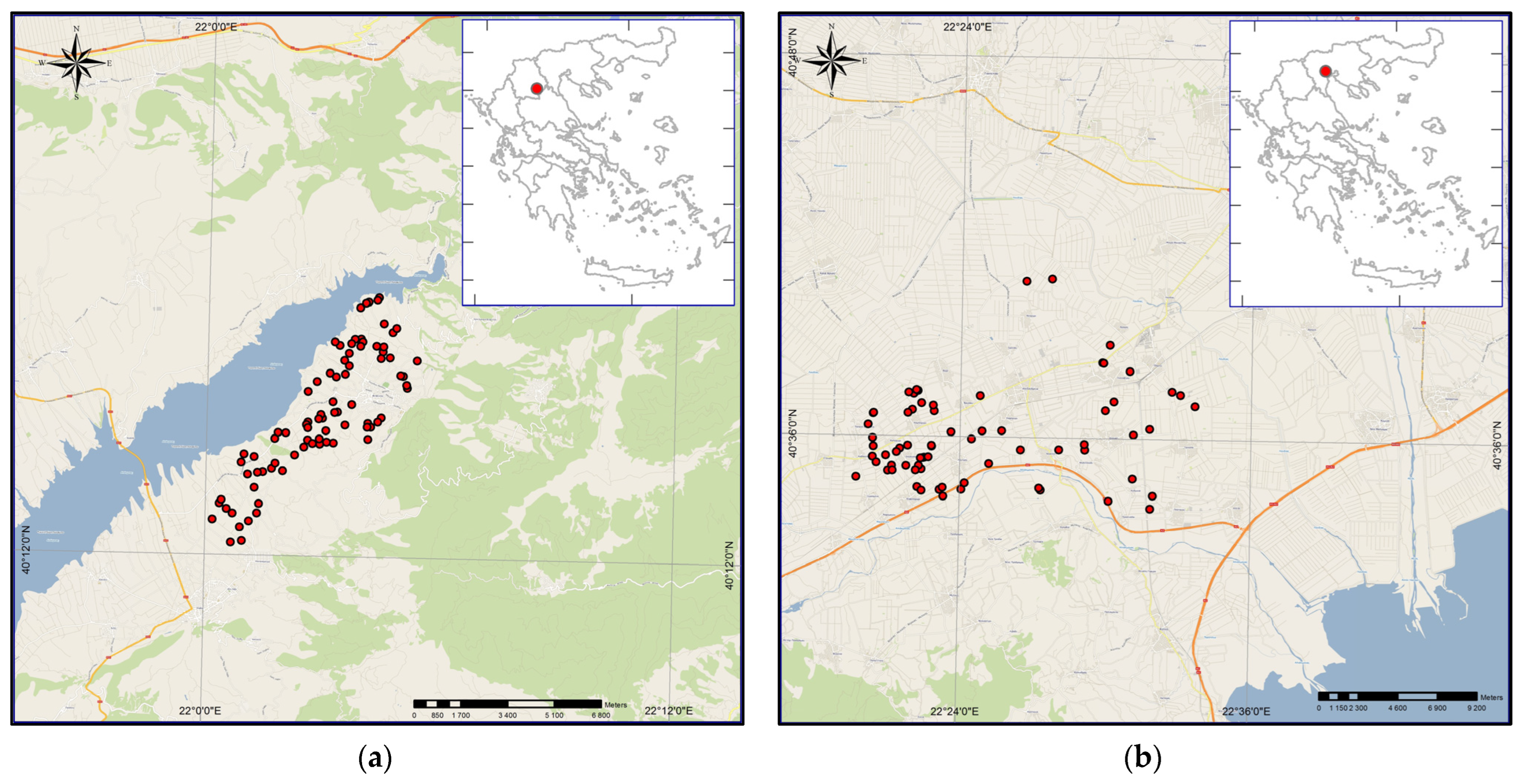
2.1. Study Area

For this study, soil samples were collected from two distinct regions in Northern Greece, namely Kozani and Veroia, each representing different geographical and climatic conditions (Figure 1). The Kozani region, specifically the Velvedos area, is situated near the shores of the artificial Lake Polyfytos, with coordinates in the World Geodetic System of 1984 (WGS84) ranging from approximately 40°47′24.00″ N to 40°51′09.00″ N latitude and 21°41′24.00″ E to 21°45′39.00″ E longitude. The terrain in this area features a considerable difference in elevation, starting at 220 m adjacent to the lake and rising to 520 m near the mountain. The climate in Kozani is characterized by temperate conditions, with cold winters and hot, dry summers. The average annual temperature is 10.8 °C, and the region receives approximately 700 mm of precipitation per year. These climatic conditions contribute to the region’s specific soil characteristics, making it an interesting subject for soil analysis.

On the other hand, Veroia, located in the Central Macedonia region, has coordinates in WGS84 ranging from approximately 40°31′48.00″ N to 40°33′36.00″ N latitude and 22°11′24.00″ E to 22°15′36.00″ E longitude. In contrast to the varied topography of Kozani, Veroia presents predominantly flat terrain with average elevation of 20 m above sea level. Its temperate climate features milder winters than Kozani, although freezing temperatures are still possible. Summers in Veroia are warm, averaging about 14 °C, and the area receives around 500 mm of annual precipitation. This distinct climate and terrain contribute to soil differences between Veroia and Kozani, providing a broader context for this study’s comparison.

2.2. Soil Sampling and Soil Data Covariates

Soil sampling was conducted in two rounds for each region, primarily in peach orchards. In September 2023, 70 soil samples were randomly collected from Veroia, while Kozani contributed 85 samples in November 2023. A second round of sampling was conducted in both regions, with Veroia providing an additional 70 samples in May 2024 and Kozani 85 more in November 2024, all from the exact same locations. The samples were dried and analyzed at the Soil and Water Resources Institute laboratory in Thessaloniki, Greece, for parameters including the bulk density, organic matter, silt, clay, and sand. To ensure representativeness, composite samples were collected from each location. Two subsamples were taken within a 3 to 5 m radius of each other, separately for both bulk density and the other soil parameters (Figure 2). GPS devices recorded the exact geographic coordinates of each sampling site for spatial reference.

The physical and organic properties of each soil sample were assessed (

Table 1. Soil parameters measured in the study.

	Parameter	Category	Unit	Method of Analysis
1	* Clay (C)	Soil	%	Particle size analysis with hydrometer
2	* Silt (Si)	Soil	%	Particle size analysis with hydrometer
3	* Sand (S)	Soil	%	Particle size analysis with hydrometer
4	* Organic Carbon (OC)	Soil	%	Walkley–Black method
5	* Bulk Density (BD)	Soil	g/cm3	Intact soil samples using a core cylinder
6	Electric Conductivity (EC)	Soil	mS/cm	In soil saturation extracts measured with conductometer
7	Acidity (pH)	Soil	---	In soil saturated paste measured with pH meter
8	Nitrate Nitrogen (NN)	Soil	ppm	With 2M KCl colorimetric with photometer
9	Phosphorus (P)	Soil	ppm	With 0.5 M NaHCO3 pH 8.5 colorimetric with photometer
10	Potassium (K)	Soil	ppm	With ammonium acetate at pH = 7.0 measured by ICP-OES
11	Magnesium (Mg)	Soil	ppm	With ammonium acetate at pH = 7.0 measured by ICP-OES
12	Iron (Fe)	Soil	ppm	DTPA ** measured by ICP-OES
13	Zinc (Zn)	Soil	ppm	DTPA ** measured by ICP-OES
14	Manganese (Mn)	Soil	ppm	DTPA ** measured by ICP-OES
15	Copper (Cu)	Soil	ppm	DTPA ** measured by ICP-OES
16	Boron (B)	Soil	ppm	Azomethine-H, colorimetric with photometer

* Parameters used in the ML_min models; ** DTPA: diethylenetriaminepentaacetic acid.

). Particle size analysis, employing the hydrometer method, was used to determine the proportions of clay, silt, and sand, thus defining the soil texture. The OC content was quantified using the Walkley–Black method [23]. The bulk density was determined on undisturbed soil cores, which were carefully extracted from a depth of 10 cm to maintain the soil structure and minimize disturbances. In general, the soils had low rock fragment content.

2.3. ML Methods and Pedotransfer Functions

The current study employed random forest (RF), cubist (CB), support vector regression (SVR), and gradient boosting (GB) as ML algorithms, selected for their established efficacy in soil parameter prediction tasks [1,9,22,24,25].

RF [26] is an ensemble learning technique that builds multiple decision trees during training. Each tree contributes a vote (classification) or mean prediction (regression), enhancing the prediction robustness and mitigating overfitting. RF’s strengths lie in its ability to manage high-dimensional data, minimize overfitting, and provide feature importance estimates. CB [27] is a rule-based model that combines decision trees with linear regression. It partitions data into subsets using rules and fits linear regression models to each subset. CB offers a balance of predictive accuracy and interpretability through its rule-based structure, aiding in understanding soil property relationships. SVR [28] is a kernel-based method that transforms input data into a higher-dimensional space, enabling the identification of non-linear relationships. It aims to find the best-fitting hyperplane within a specified margin, making it effective for both linear and non-linear regression tasks. SVR is particularly useful when dealing with complex, high-dimensional datasets. GB [29] is another ensemble technique that builds models in a stage-wise fashion, where each new model corrects the errors of the previous ones. It iteratively minimizes a loss function by adding weak learners, typically decision trees. GB is known for its high predictive accuracy and ability to capture complex interactions between features. It is a powerful method for regression tasks where high precision is required.

PTFs are vital tools in soil science and environmental studies, as they use statistical or empirical connections between easily obtainable soil characteristics like texture, organic matter, and water content to estimate the bulk density. This capability is essential in extrapolating limited field measurements to the broader spatial scales required for comprehensive soil modeling and environmental evaluations. By enabling the prediction of soil properties in areas lacking direct data, PTFs overcome data scarcity challenges. For this study, we selected five established PTFs (

Table 2. Pedotransfer functions used in the study.

	Authors	Abbrev.	Function
1	Abdelbaki [12]	AB	BD = 1.449e − 0.03OC
2	Post and Kwon [30]	PK	BD = 100/[(OM/0.244) + ((100 − OM)/MBD)]
3	Rawls, Nemes, and Pachepsky [31]	R	BD = 1.36411 + 0.185628 × (0.0845397 + 0.701658w − 0.614038w2 − 1.18871w3 + 0.0991862y − 0.301816wy − 0.153337w2y − 0.0722421y2 + 0.392736wy2 + 0.0886315y3 − 0.601301z + 0.651673wz − 1.37484w2z + 0.298823yz − 0.192686wyz + 0.0815752y2z − 0.0450214z2 − 0.179529wz2 − 0.0797412yz2 + 0.00942183z3) x = −1.2141 + 4.23123 × (Sand/100) y = −1.70126 + 7.55319 × (Clay/100) z = −1.55601 + 0.507094 × OM w = −0.0771892 + 0.256629x + 0.256704x2 − 0.140911x3 − 0.0237361y − 0.098737x2y − 0.140381y2 + 0.0140902xy2 + 0.0287001y3
4	Saxton and Rawls [11]	SR	SWC-HPC Model
5	Ruehlmann and Korschens [32]	RK	BD = (2.684 − 140.943 × 0.008) × EXP(−0.008 × OC × 10)

MBD = mineral bulk density is set to 1.64 g/cm³.

), recognized in the literature for their robust performance and consistently accurate predictions across diverse soil types [11,12,30,31,32]. This selection was further supported by the performance evaluation and ranking conducted by Sevastas et al. [33] on soils in Northern Greece, a geographically proximate area, which identified these five PTFs as yielding the most promising results.

The PTFs, due to their extensive validation and demonstrated reliability, are well suited to tackling the complexities inherent in large-scale soil property estimation. Nevertheless, it is crucial to acknowledge that the predictive accuracy of these functions can exhibit variability depending on the specific soil types and geographical regions under consideration.

2.4. Error Assessment Indices

The predictive performance of the bulk density models was evaluated using three key error assessment indices: the root mean squared error (RMSE), coefficient of determination (R-squared), and mean absolute error (MAE). These indices provide insights into the model accuracy, goodness of fit, and prediction quality, each offering distinct perspectives on model performance (

Table 3. Error assessment indices.

Metric	Equation
Mean absolute error (MAE)	$MAE={\displaystyle \frac{{\sum }_{i=1}^n\left|y_i-x_i\right|}{n}}$	(1)
Root mean square error (RMSE)	$RMSE=\sqrt{{\displaystyle \frac{{\sum }_{i=1}^n{\left[y_i-x_i\right]}^2}{n}}}$	(2)
Coefficient of determination (R2)	$R^2={\displaystyle \frac{S{S}_{res}}{S{S}_{tot}}}$	(3)
where	$S{S}_{res}={\displaystyle {\displaystyle \sum }_i}{\left(y_i-{\widehat{y}}_i\right)}^2$
and	$S{S}_{tot}={\displaystyle {\displaystyle \sum }_i}{\left(y_i-\overline{y}\right)}^2$

).

The mean absolute error (MAE) calculates the average of the absolute differences between the predicted and observed values (Equation (1)). The MAE provides a more robust measure of the average error magnitude as it treats all errors equally, without the squaring that emphasizes larger errors in the RMSE. The root mean squared error (RMSE) measures the square root of the average squared differences between the observed and predicted values, providing a direct interpretation in the same units as the data. It is particularly sensitive to large errors, as it penalizes larger deviations more than smaller ones (Equation (2)). A lower RMSE indicates better model accuracy. The R-squared (R²) quantifies the proportion of variance in the observed data explained by the model. It ranges from 0 to 1, with 1 indicating a perfect fit (Equation (3)). Higher R² values indicate a better fit and a stronger linear relationship between the predicted and actual values, reflecting the model’s ability to capture the data’s variability. While the R² is useful in comparing model fits, it can be misleading in cases of overfitting.

2.5. Software

The computational analyses for this study were primarily conducted using the R statistical programming language (version 4.x). R’s extensive ecosystem of packages provided the necessary tools for data manipulation, model development, and performance evaluation. Specifically, the caret (Classification and Regression Training) package was used to streamline the model training and evaluation processes, offering functionalities for cross-validation, hyperparameter tuning, and performance metric calculation across various ML algorithms. To implement the random forest model, the ranger package was utilized due to its computational speed and suitability for high-dimensional datasets. The xgboost package provided the gradient boosting framework for the xgbLinear model (gradient boosting), known for its high predictive accuracy. Support vector regression was implemented using the kernlab package, offering flexibility in kernel selection. Finally, the cubist package was implemented for the development of the rule-based cubist model. Data visualization was achieved using R’s base graphics and ggplot2 package, enabling the creation of informative plots for data exploration and result presentation. All analyses were performed on a standard desktop computer running a Windows-based operating system.

3. Results

3.1. Descriptive Statistics

The soil data from the two-year period (2023–2024) were combined for each area, resulting in 170 samples for Kozani and 140 for Veroia. The descriptive statistics for the Kozani region (

Table 4. Descriptive statistics of Kozani region.

	S	C	Si	pH	Ec	NN	P	K	Mg	Fe	Zn	Mn	Cu	B	OC	BD
mean	56.76	14.72	28.51	6.85	0.49	11.31	20.72	171.90	257.17	33.45	2.39	11.15	5.26	0.59	0.84	1.44
sd	13.15	9.17	6.45	0.73	0.17	6.77	13.37	102.10	158.89	32.16	1.33	6.94	3.48	0.25	0.29	0.14
median	60.00	12.00	28.00	6.95	0.45	10.32	18.98	149.00	198.00	22.35	2.25	9.23	4.56	0.56	0.82	1.45
min	12.00	2.00	16.00	4.87	0.25	2.69	3.15	50.00	60.00	4.13	0.37	2.19	0.85	0.21	0.36	1.05
max	80.00	54.00	58.00	8.08	1.27	45.18	69.47	553.00	753.00	189.80	5.80	35.62	20.47	1.71	1.64	1.78
skew	−1.18	1.79	1.14	−0.59	1.47	2.08	1.04	1.50	1.17	2.16	0.63	1.36	1.54	1.60	0.43	−0.29
kurtosis	1.44	3.78	2.87	0.00	3.06	6.27	0.92	2.27	0.61	5.47	−0.21	1.89	3.33	4.07	−0.44	−0.10

) reveal a soil environment with considerable variability, particularly in key chemical and physical properties relevant to BD prediction. Sand dominates the texture, with a high mean value (56.76%) and relatively low skewness, suggesting a moderately uniform distribution. In contrast, clay exhibits strong positive skewness (1.79) and high kurtosis (3.78), indicating that, while most samples have low clay content, a few contain substantially higher levels.

The OC levels are generally low (mean: 0.84%) and show modest variability. Chemical compounds like NN, K, Fe, Zn, and Mg display high standard deviations and strong positive skewness, highlighting their heterogeneous distribution. The negative skewness in BD (−0.29), with a relatively narrow range (1.05–1.78 g/cm³), indicates a slight tendency toward higher density values.

The descriptive statistics for Veroia (

Table 5. Descriptive statistics of Veroia region.

	S	C	Si	pH	Ec	NN	P	K	Mg	Fe	Zn	Mn	Cu	B	OC	BD
mean	19.78	31.46	48.75	7.73	1.06	21.89	14.12	466.00	525.18	20.76	1.95	26.76	6.81	0.74	1.32	1.35
sd	10.74	12.41	9.25	0.23	0.73	14.65	17.85	196.00	149.90	7.08	1.27	41.12	4.44	0.39	0.34	0.11
median	19.00	28.00	48.00	7.75	0.79	16.62	10.70	432.00	513.50	19.16	1.70	13.96	5.92	0.66	1.31	1.35
min	4.00	4.00	20.00	6.61	0.45	1.67	2.39	137.00	144.00	9.70	0.23	6.00	1.40	0.14	0.72	1.08
max	60.00	62.00	74.00	8.15	5.64	54.07	180.02	1357.00	988.00	52.29	7.54	247.80	31.28	2.56	2.79	1.63
skew	0.90	0.56	−0.07	−1.50	2.83	0.67	6.52	1.19	0.50	1.57	1.91	3.61	2.19	1.56	0.82	0.01
kurtosis	0.92	−0.61	−0.30	4.33	11.24	−0.88	53.39	2.34	0.76	3.17	4.67	13.28	7.05	4.50	1.65	−0.54

) present a different soil profile compared to Kozani, characterized by a finer texture and a significantly richer chemical environment. Silt dominates the particle size distribution, with a mean of 48.75%, while the sand content is substantially lower (mean: 19.78%), indicating soils that are more moisture-retentive and potentially more stable structurally.

The OC levels are notably higher (mean: 1.32%) and display moderate variability, suggesting a generally fertile soil base. Ec shows high skewness (2.83) and kurtosis (11.24), pointing to a few samples with elevated salinity, which may affect the BD. The nutrient concentrations, particularly NN, K, and Mg, are substantially elevated compared to Kozani, with K peaking at 1357 mg/kg. The extreme kurtosis and skewness values in elements like P (kurtosis: 53.39) and Mn (kurtosis: 13.28) underscore the presence of outliers and considerable heterogeneity. Despite this chemical richness, the BD in Veroia remains narrowly distributed (mean: 1.35 g/cm³, SD: 0.11), with negligible skewness.

3.2. Prediction Results

Each dataset was split into training (80%) and testing (20%) subsets. The training data were used to build the ML models, while the testing data were used to evaluate the predictive accuracy by comparing the observed and predicted soil BD. The same testing subset was also used to assess the performance of the PTFs.

All four predictive models—random forest (ranger), XGBoost linear (xgbLinear), support vector regression (svmLinear), and cubist—were developed using the caret package with a consistent evaluation strategy of repeated 10-fold cross-validation (number = 10, repeats = 3) to ensure robust generalization. This cross-validation strategy involved partitioning the training data into 10 distinct subsets, iteratively training on nine and validating on one, which was repeated three times to mitigate variability in the performance estimates and increase the reliability of the models. In addition to this, multiple trials were conducted by setting different random seed values (ranging from 1 to 40), which also affected the data splitting (training–testing), to further minimize any potential bias in the results, ensuring that the model performance was not overly influenced by a particular initial random state. Each model underwent hyperparameter tuning through a random search (search = ‘random’, tuneLength = 30), which explored 30 random combinations of parameter values, aiming to identify the optimal configuration for each algorithm. The models’ predictive performance was quantified using the root mean squared error (RMSE), and the objective was to minimize this metric during the training process to ensure the most accurate predictions. The SVR model additionally involved pre-processing steps of centering and scaling the predictor variables to standardize their distributions, ensuring the model’s efficiency in handling features with varying scales.

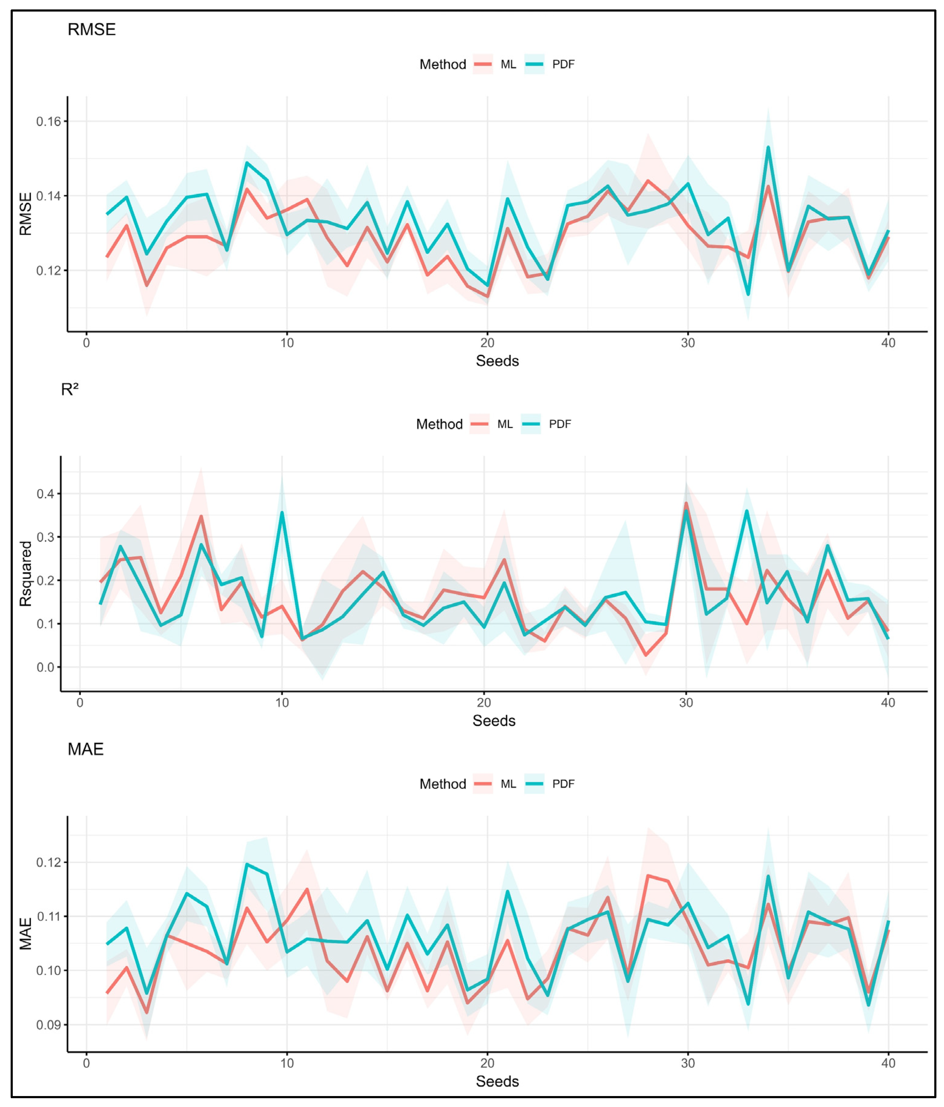
3.2.1. Kozani Dataset—PTFs vs. ML_min (C, Si, S, OC)

In the Kozani area, the comparison between PTFs and ML models in predicting BD using with the same parameters (C, Si, S, OC), reveals marginal performance differences, although some trends emerge (

Table 6. Comparison of predictive accuracy for BD using PTFs and ML_min in the Kozani area.

PTFs				ML_min
Method	RMSE	MAE	R2	Method	RMSE	MAE	R2
AB	0.137	0.110	0.14	CB	0.131	0.106	0.13
PK	0.138	0.110	0.14	RF *	0.125	0.101	0.19
R	0.131	0.104	0.15	SVR	0.130	0.104	0.13
SR	0.128	0.102	0.23	GB	0.129	0.105	0.19
RK	0.129	0.104	0.14
Average	0.133	0.106	0.16	Average	0.129	0.104	0.16

* Best model overall.

). On average, ML models slightly outperform PTFs, with a lower RMSE (0.129 vs. 0.133) and MAE (0.104 vs. 0.106), while both approaches yield an identical mean R² of 0.16.

Among the PTFs, SR performs best, achieving the highest R² (0.23) and the lowest RMSE (0.128), indicating its relative effectiveness within the traditional modeling framework. On the ML side, the RF and GB models stand out, both achieving the highest R² (0.19) and maintaining competitive RMSE and MAE values. Notably, while ML—particularly ensemble methods like RF and GB—offers slight improvements in accuracy, the gains are not substantial, suggesting that, in this specific context, traditional PTFs (SR) remain robust and competitive.

Regarding the performance across all seeds, we have to keep in mind that the effectiveness of both ML and PTFs is influenced by the random seed. For ML, this affects the model’s initial parameters and learning process. Crucially, the seed also determines the 80% of the data that are used for training and the 20% used for testing in each of the 40 trials, thus impacting the evaluation results for both types of methods.

Visually (Figure 3), the ML line (red) and the PTF line (blue) tend to follow a similar overall trend for all three metrics (RMSE, R², and MAE). This reinforces the idea that, on average, their performance is comparable. When one line shows an increase or decrease, the other often mirrors this behavior to some extent. However, in general, the ML models slightly outperform the PTFs across most seeds, with lower RMSE and MAE values and higher R² scores.

3.2.2. Kozani Dataset—PTFs vs. ML

In the case of ML models that incorporate a comprehensive set of soil properties (e.g., texture, nutrients, pH, micronutrients), they significantly outperform traditional PTFs in predicting the soil bulk density in the Kozani area (

Table 7. Comparison of predictive accuracy for BD using PTFs and ML in the Kozani area.

PTFs				ML
Method	RMSE	MAE	R2	Method	RMSE	MAE	R2
AB	0.137	0.110	0.14	CB	0.124	0.102	0.25
PK	0.138	0.110	0.14	RF *	0.114	0.092	0.33
R	0.131	0.104	0.15	SVR	0.124	0.100	0.22
SR	0.128	0.102	0.23	GB	0.126	0.102	0.25
RK	0.129	0.104	0.14
Average	0.133	0.106	0.16	Average	0.122	0.099	0.26

* Best model overall.

).

The average RMSE and MAE for ML methods were 0.122 and 0.099, respectively, clearly lower than the PTF averages of 0.133 (RMSE) and 0.106 (MAE). More strikingly, ML achieved an average R² of 0.26—over 60% higher than the PTFs (0.16)—indicating a notably better ability to explain the variability in the data. Among the ML models, RF was the top performer, with the lowest RMSE (0.114), the lowest MAE (0.092), and the highest R² (0.33). GB and CB also delivered strong results, with R² values of 0.25. In contrast, the best PTF method, SR, reached a maximum R² of 0.23.

Visually examining the performance across all seeds, the ML models (red line) increasingly outperform the PTFs (blue line) when utilizing the full parameter set (Figure 4). This trend is more pronounced than with the minimal parameter set, as evidenced by the generally lower RMSE and MAE values and higher R² scores for ML across most of the seeds.

These results suggest that ML models leveraging multiple soil parameters noticeably enhance the predictive performance. This reinforces the value of data-rich approaches and highlights that ML is especially powerful when multi-variable soil data are available.

The variance importance scores (top ten) for the best RF model reveal some key findings about the predictors of soil BD (Figure 5). Zn emerges as the most influential variable in the Kozani dataset. This exceptionally high score suggests that Zn plays a dominant role in predicting the BD, far surpassing all other variables. Such a finding is atypical, as the BD is usually more closely linked to soil properties like OM, S, C, and Si.

Following Zn, OC and NN are the next most important predictors, with scores of 46.36% and 32.77%, respectively. This suggests that OM and NN both have substantial roles in shaping the BD predictions, with OC contributing to the overall soil quality and NN influencing soil fertility, both of which are linked to the BD. Other important variables include S and K, with scores of 25.23% and 22.33%, respectively, indicating that these soil parameters also have a significant, but less dominant, effect on BD predictions. Additionally, elements such as Mg, Si, and Mn, while contributing moderately to the model (ranging from 11% to 15%), still show some importance in the prediction process. Lastly, C and Fe have the smallest impacts on the model, with variance scores of 8.42% and 5.21%, respectively.

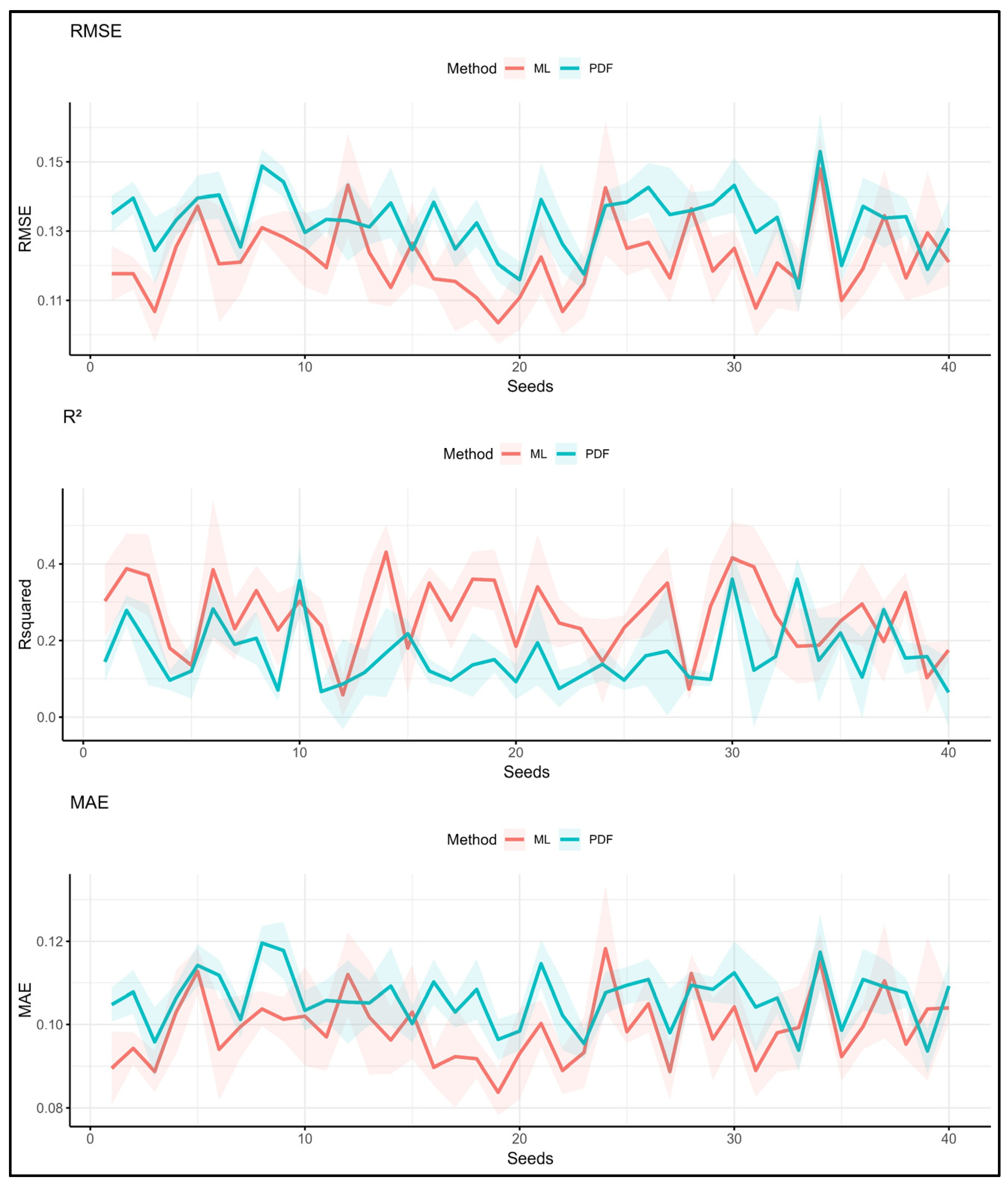
3.2.3. Veroia Dataset—PTFs vs. ML_min (C, Si, S, OC)

Initially, the results from the Veroia area are presented, where both PTFs and ML models were developed using the same limited set of soil parameters: sand, silt, clay, and organic carbon. ML models built using basic soil parameters demonstrate an advantage in reducing the prediction error for BD compared to traditional PTFs (

Table 8. Comparison of predictive accuracy for BD using PTFs and ML_min in Veroia area.

PTFs				ML_min
Method	RMSE	MAE	R2	Method	RMSE	MAE	R2
AB	0.110	0.091	0.36	CB	0.091	0.074	0.33
PK	0.118	0.098	0.36	RF	0.093	0.076	0.31
R	0.091	0.076	0.35	SVR *	0.089	0.073	0.37
SR	0.096	0.077	0.34	GB	0.098	0.079	0.24
RK	0.105	0.088	0.36
Average	0.104	0.086	0.35	Average	0.093	0.076	0.31

* Best model overall.

). The average RMSE for ML models is 0.093, noticeably lower than the 0.104 recorded for the PTFs, marking a meaningful improvement in predictive accuracy. Similarly, the average MAE decreases from 0.086 (PTFs) to 0.076 (ML), further highlighting the greater precision of ML approaches under these conditions. While the PTFs show a slightly higher average R² (0.35 vs. 0.31), the substantial reduction in the RMSE with ML is particularly significant, as it reflects improved prediction accuracy.

Among the ML models, SVR performs best, with the highest R² (0.37) and the lowest RMSE (0.089), slightly outperforming the best PTF method, which is R, with an R² of 0.35 and RMSE of 0.091. These results suggest that, even when limited to a narrow set of inputs, ML models—especially SVR—can offer a measurable gain in prediction accuracy over PTFs in this specific case.

Across the 40 trials (Figure 6) in the Veroia area using limited parameters (C, Si, S, OC), ML models (red line) tend to outperform PDFs (blue line) across most data splits in terms of the RMSE and MAE. For example, in the RMSE diagram, the ML line is visually lower most of the time, indicating smaller prediction errors. This contrasts with the Kozani area under the same limited parameters, where the performance difference between ML and PTFs is less pronounced and consistent. In the case of the R², the PDFs and ML exhibit similar prediction accuracy.

3.2.4. Veroia Dataset—PTFs vs. ML

In Veroia, when ML models are trained using an expanded set of soil parameters—including texture, organic carbon, pH, electrical conductivity, macronutrients (e.g., nitrate nitrogen, phosphorus, potassium), and micronutrients (e.g., Fe, Zn, Mn, Cu, B)—they show a moderate improvement in predictive errors but a decline in explained variance compared to traditional PTFs (

Table 9. Comparison of predictive accuracy for BD using PTFs and ML in Veroia area.

PTFs				ML
Method	RMSE	MAE	R2	Method	RMSE	MAE	R2
AB	0.110	0.091	0.36	CB	0.093	0.077	0.30
PK	0.118	0.098	0.36	RF	0.092	0.075	0.32
R *	0.091	0.076	0.35	SVR	0.096	0.078	0.27
SR	0.096	0.077	0.34	GB	0.099	0.081	0.24
RK	0.105	0.088	0.36
Average	0.104	0.086	0.35	Average	0.095	0.078	0.28

* Best model overall.

). The average RMSE of the ML models decreases from 0.104 (PTFs) to 0.095, and the MAE drops from 0.086 to 0.078, indicating better alignment between the predicted and observed BD values. However, the average R² for the ML models falls to 0.28, compared to 0.35 for the PTFs, suggesting that the added variables do not substantially increase the models’ explanatory power.

Among the ML methods, RF performs best, with an RMSE of 0.092 and R² of 0.32, slightly improving the accuracy but still trailing behind the PTFs in terms of the variance explained. Notably, R from the PTFs outperforms all other models overall, achieving the lowest RMSE (0.091) and a strong R² (0.35). These findings imply that, while the inclusion of more soil variables helps to reduce prediction errors, it does not necessarily enhance the model interpretability or explanatory strength in this context.

Examining the 40 trials (Figure 7) for the Veroia area with the full parameter set shows a clear trend of the ML models (red line) consistently outperforming the PDFs (blue line) in terms of the RMSE and MAE. However, this advantage does not extend to the R², where the PTFs tend to yield better results. Compared to the limited parameter scenario in Veroia, increasing the number of parameters does not appear to improve the ML performance and seems to increase the variability, as indicated by the more frequent intersections between the red and blue lines.

Regarding the variance importance scores (top ten) for the best RF model in Veroia (Figure 8), OC stands out as the most important variable, contributing significantly to the prediction of BD, with a variance importance score of 100%. This suggests that OC is the most influential predictor of BD in the Veroia dataset. Following OC, the K and sand content (S) are the next most important predictors, with scores of 41.97% and 37.21%, respectively. These findings suggest that K and S also play a significant role in determining BD, although to a lesser extent than OC.

Other variables like Cu, Si, Ec, and the pH also have notable importance, with variance scores ranging from 15% to 20%. This indicates that these soil properties also contribute to the model’s predictive power, although their importance is secondary to that of the top three variables (OC, K, and S). The remaining variables, including Zn, Mn, and Fe, are less important, with scores ranging from 9% to 15%.

4. Discussion

The preceding results offer valuable insights into the prediction of the bulk density (BD) across two distinct agricultural regions, Veroia and Kozani, utilizing both ML models and traditional PTFs under varying data availability. The observed regional disparities in prediction accuracy, the comparative performance of ML versus PTFs, and the nuanced impact of the dataset size (“full” vs. “min”) warrant a more in-depth discussion.

4.1. Regional Differences (Veroia vs. Kozani)

In terms of overall prediction accuracy, Veroia outperforms Kozani across all models when using the full dataset (Figure 9). This is evident in the lower RMSE and MAE values for Veroia, indicating that the model predictions in this region are more precise and closer to the actual values. Additionally, Veroia’s R² value is higher, signifying that the models better capture the underlying relationship between the soil properties and the features used for prediction. In contrast, Kozani’s models exhibit slightly less accurate predictions, with a higher RMSE and MAE and a marginally lower R². This suggests that the soil properties in Veroia may follow more consistent patterns or are more easily modeled, whereas Kozani’s soil data present greater complexity or noise that the models find harder to predict.

Veroia’s soil seems to be more homogeneous due to consistent pedogenic processes (predominantly flat terrain), allowing the models to capture the relationships between the predictors and bulk density (BD) more effectively. In contrast, Kozani’s heterogeneous soils, influenced by diverse geological and topographical factors (close to the lake, with a considerable difference in elevation), pose a greater challenge for accurate BD prediction. The variable importance analysis reveals that Zn is the key predictor in Kozani, suggesting a chemically driven soil environment. Conversely, OC, K, and S are the most influential in Veroia, indicating that BD is more strongly governed by basic textural and organic matter parameters.

4.2. ML vs. PTF Performance

In both the Veroia and Kozani datasets, ML models generally achieve lower prediction errors compared to PTFs. For Veroia, ML yields a better RMSE (0.095 vs. 0.104) and MAE (0.078 vs. 0.086) than PTFs, although PTFs have a higher R² (0.35 vs. 0.28), suggesting that they explain more variance despite larger errors. In Kozani, ML also outperforms PTFs in the “full” dataset (RMSE: 0.122 vs. 0.133; R²: 0.26 vs. 0.16), but the performance is nearly identical in the “min” dataset, as seen by the red dotted line (Figure 9).

The general trend of the ML models outperforming the PTFs in terms of the RMSE and MAE aligns with our expectations, given ML’s ability to capture complex non-linear relationships. However, the higher R² values observed for the PTFs in some instances, particularly in Veroia, suggest that PTFs, despite having larger errors, might be better at explaining the overall variance in BD. This highlights a crucial trade-off between prediction accuracy and explanatory power. PTFs, with their simpler structure, might capture the broad, underlying trends, while ML models, although minimizing errors, could exhibit overfitting to noise in the data, leading to a slightly reduced capacity to generalize. Finally, the near-identical performance of ML and PTFs with the “min” dataset in Kozani further emphasizes that the advantage of ML is contingent on data availability, a theme that is further explored in the subsequent section.

4.3. Impact of Dataset Size (“Full” vs. “Min”)

Expanding the input variables in ML models significantly improves BD prediction in the Kozani area. When using only basic soil properties—sand, silt, clay, and organic carbon—ML models show only slight gains over traditional PTFs (red dotted line, PDF RMSE: 0.133, R²: 0.16 vs. ML_min RMSE: 0.129, R²: 0.16). However, when additional parameters such as the pH, electrical conductivity, nitrate nitrogen, phosphorus, potassium, and micronutrients like Zn and Fe are included, the ML performance improves substantially, as represented by the green line in Figure 9 (ML RMSE: 0.122, R²: 0.26). This highlights ML’s strength in handling complex, high-dimensional data, unlike PTFs, which are limited by their simpler structure. These results show that ML’s advantage is data-dependent: it offers clear benefits when rich soil datasets are available. In the Kozani area, when the input is restricted, well-calibrated PTFs can perform nearly as well, emphasizing their robustness under controlled conditions.

A counterintuitive result was observed in Veroia (Figure 9), where the inclusion of more variables led to a slight decrease in model performance (red dotted line vs. green line, ML_min RMSE: 0.093, R²: 0.31 vs. ML RMSE: 0.095, R²: 0.28). This outcome suggests that, in this specific region, the basic soil properties already explain a substantial portion of the variation in BD. The additional variables, rather than providing new predictive information, might be introducing noise, redundancy, or even multicollinearity, which can negatively impact model performance. This finding highlights a critical principle in ML: more data does not always translate to better performance. Thoughtful feature selection, guided by an understanding of the underlying soil processes, is crucial in building efficient and effective predictive models.

5. Conclusions

The current study compared the performance of traditional PTFs and ML algorithms in predicting the soil bulk density (BD) across two contrasting agricultural regions in Greece—Kozani and Veroia—under both limited and expanded sets of soil input variables.

This study revealed significant regional disparities in soil BD prediction, with Veroia consistently outperforming Kozani across all models. This suggests that the more homogeneous soil properties in Veroia result in more accurate modeling. In contrast, Kozani’s more varied geology and topography, including its proximity to a lake and significant altitude changes, appear to increase the soil heterogeneity, which makes predicting the BD more difficult. While ML generally showed superior prediction accuracy (lower RMSE and MAE) compared to the PTFs, especially with rich datasets, the PTFs sometimes exhibited higher R² values, indicating their potential to capture broad trends despite larger errors. This underscores a crucial trade-off between minimizing prediction errors and explaining variance. Ultimately, the impact of the dataset size is highly context-dependent; expanding the input variables significantly improved the ML performance in Kozani, demonstrating ML’s strength with high-dimensional data, whereas, in Veroia, additional variables seemed to introduce noise, emphasizing the importance of thoughtful feature selection.

In summary, our results reveal the following important insights. (1) Regional specificity is important: soil property prediction models must be tailored to the unique pedological, geological, and topographical characteristics of a region for optimal performance. A “one-size-fits-all” approach is insufficient. (2) Data richness empowers ML, but quality over quantity is needed: while ML thrives on comprehensive datasets, particularly for complex soil environments, simply adding more variables without careful consideration can introduce noise and hinder model performance. (3) Balancing accuracy and interpretability is essential: the choice between ML and PTFs depends on the specific objective. ML can offer higher predictive accuracy with low prediction errors, especially when an RMSE-minimizing optimization is employed, but PTFs can sometimes provide better explanatory power regarding the overall variance, which might be valuable in understanding the underlying soil processes. (4) PTFs remain robust in data-limited scenarios: despite ML’s general superiority, in some cases, PTFs can offer comparable performance to ML models when only a minimal set of soil properties is available.

To build on our findings and further verify the results, future research should prioritize using larger and more diverse datasets from various regions. Finally, automated feature selection and dimensionality reduction could be explored to optimize the model complexity and prevent overfitting in expanded datasets.

References

1. Ramcharan, A.; Hengl, T.; Beaudette, D.; Wills, S. A Soil Bulk Density Pedotransfer Function Based on Machine Learning: A Case Study with the NCSS Soil Characterization Database. Soil Sci. Soc. Am. J. 2017, 81, 1279–1287. [Google Scholar] [CrossRef]
2. Lai, R.; Kimble, J. Importance of soil bulk density and methods of its importance. In Assessment Methods for Soil Carbon; CRC Press: Boca Raton, FL, USA, 2000; Volume 31. [Google Scholar]
3. Hillel, D. Introduction to Environmental Soil Physics; Elsevier: Amsterdam, The Netherlands, 2003. [Google Scholar]
4. Schaetzl, R.; Anderson, S. Soils: Genesis and Geomorphology; Cambridge University Press: New York, NY, USA, 2015. [Google Scholar]
5. Reichert, J.M.; Suzuki, L.E.A.S.; Reinert, D.J.; Horn, R.; Håkansson, I. Reference bulk density and critical degree-of-compactness for no-till crop production in subtropical highly weathered soils. Soil Tillage Res. 2009, 102, 242–254. [Google Scholar] [CrossRef]
6. Walter, K.; Don, A.; Tiemeyer, B.; Freibauer, A. Determining Soil Bulk Density for Carbon Stock Calculations: A Systematic Method Comparison. Soil Sci. Soc. Am. J. 2016, 80, 579–591. [Google Scholar] [CrossRef]
7. Xu, L.; He, N.P.; Yu, G.R.; Wen, D.; Gao, Y.; He, H.L. Differences in pedotransfer functions of bulk density lead to high uncertainty in soil organic carbon estimation at regional scales: Evidence from Chinese terrestrial ecosystems. J. Geophys. Res. Biogeosci. 2015, 120, 1567–1575. [Google Scholar] [CrossRef]
8. Blanco, H.; Lal, R. Principles of Soil Conservation and Management; Springer: New York, NY, USA, 2008; Volume 167169. [Google Scholar]
9. Panagos, P.; De Rosa, D.; Liakos, L.; Labouyrie, M.; Borrelli, P.; Ballabio, C. Soil bulk density assessment in Europe. Agric. Ecosyst. Environ. 2024, 364, 108907. [Google Scholar] [CrossRef]
10. Benites, V.M.; Machado, P.L.O.A.; Fidalgo, E.C.C.; Coelho, M.R.; Madari, B.E. Pedotransfer functions for estimating soil bulk density from existing soil survey reports in Brazil. Geoderma 2007, 139, 90–97. [Google Scholar] [CrossRef]
11. Saxton, K.E.; Rawls, W.J. Soil Water Characteristic Estimates by Texture and Organic Matter for Hydrologic Solutions. Soil Sci. Soc. Am. J. 2006, 70, 1569–1578. [Google Scholar] [CrossRef]
12. Abdelbaki, A.M. Evaluation of pedotransfer functions for predicting soil bulk density for US soils. Ain Shams Eng. J. 2018, 9, 1611–1619. [Google Scholar] [CrossRef]
13. Holmes, K.W.; Wherrett, A.; Keating, A.; Murphy, D.V. Meeting bulk density sampling requirements efficiently to estimate soil carbon stocks. Soil Res. 2012, 49, 680–695. [Google Scholar] [CrossRef]
14. Zhou, W.; Guan, K.; Peng, B.; Margenot, A.; Lee, D.; Tang, J.; Jin, Z.; Grant, R.; DeLucia, E.; Qin, Z.; et al. How does uncertainty of soil organic carbon stock affect the calculation of carbon budgets and soil carbon credits for croplands in the U.S. Midwest? Geoderma 2023, 429, 116254. [Google Scholar] [CrossRef]
15. Grossman, R.; Reinsch, T. 2.1 Bulk density and linear extensibility. In Methods of Soil Analysis: Part 4 Physical Methods; John Wiley & Sons: New York, NY, USA, 2002; Volume 5, pp. 201–228. [Google Scholar]
16. Bouma, J. Using soil survey data for quantitative land evaluation. In Advances in Soil Science; Springer: New York, NY, USA, 1989; Volume 9, pp. 177–213. [Google Scholar]
17. De Vos, B.; Van Meirvenne, M.; Quataert, P.; Deckers, J.; Muys, B. Predictive Quality of Pedotransfer Functions for Estimating Bulk Density of Forest Soils. Soil Sci. Soc. Am. J. 2005, 69, 500–510. [Google Scholar] [CrossRef]
18. de Castro Moreira da Silva, L.; Amorim, R.S.S.; Fernandes Filho, E.I.; Bocuti, E.D.; da Silva, D.D. Pedotransfer functions and machine learning: Advancements and challenges in tropical soils. Geoderma Reg. 2023, 35, e00720. [Google Scholar] [CrossRef]
19. Chirico, G.B.; Medina, H.; Romano, N. Functional evaluation of PTF prediction uncertainty: An application at hillslope scale. Geoderma 2010, 155, 193–202. [Google Scholar] [CrossRef]
20. Goidts, E.; Van Wesemael, B.; Crucifix, M. Magnitude and sources of uncertainties in soil organic carbon (SOC) stock assessments at various scales. Eur. J. Soil Sci. 2009, 60, 723–739. [Google Scholar] [CrossRef]
21. Alaboz, P.; Demir, S.; Dengiz, O. Assessment of Various Pedotransfer Functions for the Prediction of the Dry Bulk Density of Cultivated Soils in a Semiarid Environment. Commun. Soil Sci. Plant Anal. 2021, 52, 724–742. [Google Scholar] [CrossRef]
22. Xiao, Y.; Xue, J.; Zhang, X.; Wang, N.; Hong, Y.; Jiang, Y.; Zhou, Y.; Teng, H.; Hu, B.; Lugato, E.; et al. Improving pedotransfer functions for predicting soil mineral associated organic carbon by ensemble machine learning. Geoderma 2022, 428, 116208. [Google Scholar] [CrossRef]
23. Nelson, D.W.; Sommers, L.E. Total carbon, organic carbon, and organic matter. Methods Soil Anal. Part 3 Chem. Methods 1996, 5, 961–1010. [Google Scholar]
24. Gunarathna, M.H.J.P.; Sakai, K.; Nakandakari, T.; Momii, K.; Kumari, M.K.N. Machine Learning Approaches to Develop Pedotransfer Functions for Tropical Sri Lankan Soils. Water 2019, 11, 1940. [Google Scholar] [CrossRef]
25. Nikou, M.; Tziachris, P. Prediction and Uncertainty Capabilities of Quantile Regression Forests in Estimating Spatial Distribution of Soil Organic Matter. ISPRS Int. J. Geo-Inf. 2022, 11, 130. [Google Scholar] [CrossRef]
26. Breiman, L. Random forests. Mach. Learn. 2001, 45, 5–32. [Google Scholar] [CrossRef]
27. Wang, Y.; Witten, I.H. Inducing model trees for continuous classes. In Proceedings of the Ninth European Conference on Machine Learning, Prague, Czech Republic, 23–25 April 1997; pp. 128–137. [Google Scholar]
28. Cortes, C.; Vapnik, V. Support-vector networks. Mach. Learn. 1995, 20, 273–297. [Google Scholar] [CrossRef]
29. Friedman, J.H. Greedy function approximation: A gradient boosting machine. Ann. Stat. 2001, 29, 1189–1232. [Google Scholar] [CrossRef]
30. Post, W.M.; Kwon, K.C. Soil carbon sequestration and land-use change: Processes and potential. Glob. Change Biol. 2000, 6, 317–327. [Google Scholar] [CrossRef]
31. Rawls, W.J.; Nemes, A.; Pachepsky, Y. Effect of soil organic carbon on soil hydraulic properties. Dev. Soil Sci. 2004, 30, 95–114. [Google Scholar]
32. Ruehlmann, J.; Körschens, M. Calculating the effect of soil organic matter concentration on soil bulk density. Soil Sci. Soc. Am. J. 2009, 73, 876–885. [Google Scholar] [CrossRef]
33. Sevastas, S.; Gasparatos, D.; Botsis, D.; Siarkos, I.; Diamantaras, K.I.; Bilas, G. Predicting bulk density using pedotransfer functions for soils in the Upper Anthemountas basin, Greece. Geoderma Reg. 2018, 14, e00169. [Google Scholar] [CrossRef]
Figure 1. Areas of study with the soil sample locations. (a) Kozani region, (b) Veroia region.
Agriculture 15 01134 g001
Figure 2. Soil sampling on the field.
Agriculture 15 01134 g002
Figure 3. Prediction results of PDFs and ML for Kozani area using the minimum dataset (C, Si, S, OC) across all seeds.
Agriculture 15 01134 g003
Figure 4. Prediction results of PDFs and ML for Kozani area using the full dataset across all seeds.
Agriculture 15 01134 g004
Figure 5. Variance importance scores (top ten) for the best RF model in the Kozani area (full dataset).
Agriculture 15 01134 g005
Figure 6. Prediction results of PDFs and ML for the Veroia area using the minimum dataset (C, Si, S, OC) across all seeds.
Agriculture 15 01134 g006
Figure 7. Prediction results of PDFs and ML for Veroia area using the full dataset across all seeds.
Agriculture 15 01134 g007
Figure 8. Variance importance scores (top ten) for the best RF model in the Veroia area (full dataset).
Agriculture 15 01134 g008
Figure 9. Comparative performance metrics by method and area. Lines present performance shifts across methods for each area.
Agriculture 15 01134 g009