CFD-Based Flow Field Characteristics of Air-Assisted Sprayer in Citrus Orchards

Abstract

Air-assisted sprayers are an essential piece of equipment for improving spraying efficiency and pesticide utilization; their performance directly affects the effectiveness of pesticide application. This study, addressing the plant protection needs of hilly citrus orchards, designed an air duct structure for an air-assisted sprayer and analyzed its airflow characteristics and droplet deposition effects based on CFD simulation technology. The reliability of the simulation results was verified through air speed boundary tests, revealing that the maximum effective boundaries of the integrated air duct and the independent air duct in different directions were 18.4 cm and 17.2 cm, respectively, providing a reference for the spatial arrangement of the air duct. The study indicates that properly matching the fan speed, spray pressure, and spray distance could optimize droplet deposition, enhance spray uniformity, and improve pesticide utilization. However, excessively high fan speeds (>6000 r/min) or spray pressures (>0.8 MPa) may reduce droplet transport efficiency. This research provides theoretical support for the design and parameter optimization of sprayers in hilly citrus orchards.

1. Introduction

In agricultural production, plant protection operations are a fundamental production process, a key factor affecting environmental quality, and an influence on dietary health [1,2]. These operations account for 30% of the total field management workload in orchards [3,4]. Achieving on-demand precision spraying, variable-rate application, and separation of humans from both machinery and pesticides, as well as developing efficient and intelligent spraying equipment, are essential for improving the efficiency of plant protection operations and pesticide utilization [5,6]. Additionally, these measures play a crucial role in ensuring food safety and reducing farmers’ labor intensity. To reduce the exposure risk of operators, fixed spraying systems and UAV-based spraying systems are currently under evaluation. However, these technologies face challenges in hilly and mountainous orchard environments due to terrain constraints [7,8].

Air-assisted sprayers, as essential equipment for improving spraying efficiency and pesticide utilization, have received widespread attention [9,10]. Existing studies have shown that the axial fan, nozzles, and spray-guiding devices significantly influence sprayer performance [11]. To further enhance spray effectiveness and droplet deposition uniformity, research has focused on optimizing air duct design, analyzing airflow characteristics, and refining spray parameters [12,13]. Based on CFD simulation technology, researchers have explored the impact of different air duct structures and operating conditions on droplet deposition by simulating various combinations [14,15]. The performance of air-assisted sprayers is primarily affected by the axial fan, spray pressure, nozzles, and spray-guiding devices [16,17]. Khot et al. [18] developed a sprayer utilizing an axial fan for airflow, equipped with adjustable louvers that regulate airflow angle and volume by altering the louver opening angle, specifically designed for precision spraying in citrus orchards. Jing et al. [19] designed a curved air outlet suitable for axial fan air-assisted systems and conducted comparative analyses of internal airflow fields using CFD numerical simulations and experimental validation. Li et al. [20], considering the planting patterns and agronomic characteristics of walnut orchards, used CFD simulations to design an orchard sprayer equipped with five spray tubes on one side, achieving droplet coverage rates of 74.92%, 90.01%, and 69.9% for the upper, middle, and lower tree canopies, respectively. Air-assisted spray-guiding devices can influence airflow velocity and distribution, thereby indirectly affecting droplet deposition uniformity. Fan et al. [21] added several guiding devices to a sprayer and performed numerical simulations to analyze their effects at different installation angles. The optimal angles for the upper and lower air outlets and internal guiding devices were determined, increasing the average airflow velocity within the 1.6–2.4 m height range by 18.81%. Guo et al. [22] addressed insufficient foliar deposition coverage in tomato orchards by designing a vertical spray-bar electrostatic sprayer that combines multi-nozzle vertical spray bars with electrostatic spraying technology. They employed a multi-factor response surface method to investigate key influencing factors such as electrostatic voltage, spray pressure, and target distance. Xue et al. [23] developed a novel air-assisted electrostatic sprayer for hilly citrus orchards to improve the poor deposition performance of conventional spraying equipment used in such terrains. The optimal spraying parameters were determined using an orthogonal experimental method. Zhang et al. [24] simulated the complex interactions between the airflow discharged from an air-assisted sprayer and the surrounding environment, analyzing the effects of upper and lower guide vane length and installation angle on airflow distribution. Hong et al. [25] utilized a CFD simulation analysis database to construct an air-assisted spraying model and a canopy model to evaluate spray quality, aiding sprayers in making optimal pesticide application decisions. Cui et al. [26] established a three-dimensional plant model and conducted discrete particle tracking simulations to analyze droplet deposition in deformed plant canopies under gas–liquid interactions. Wang et al. [27] designed an experimental device composed of an air delivery system, a measurement system, and a fixation system. By studying the dynamic changes of peach tree leaves under different airflow conditions, they simulated leaf motion during field spraying using control experiments.

In plant protection operations, the development and optimization of precision spraying technology are of great significance, especially in the application of air-assisted sprayers. How to improve droplet deposition effectiveness through the rational design of the air duct and the adjustment of fan speed, spray pressure, and spray distance has become a key research focus [28,29]. Previous studies have shown that the structure and arrangement of sprayer components directly impact spraying performance [30], and that optimizing the sprayer’s design can effectively improve pesticide utilization and spray uniformity. However, despite extensive research on these parameters, a critical challenge remains in comprehensively considering the interactions among these factors in practical applications and further optimizing operational conditions.

This paper introduces an air-assisted sprayer for pesticide application in hilly citrus orchards. By combining CFD simulation technology and experimental verification, the study investigates the impact of the air duct structure on airflow and droplet deposition in the air-assisted sprayer. A wind-driven spraying coupling model is established to analyze the effects of fan speed, spray pressure, and spray distance on droplet deposition and spraying patterns, providing a scientific basis for practical applications [31,32,33].

2. Materials and Methods

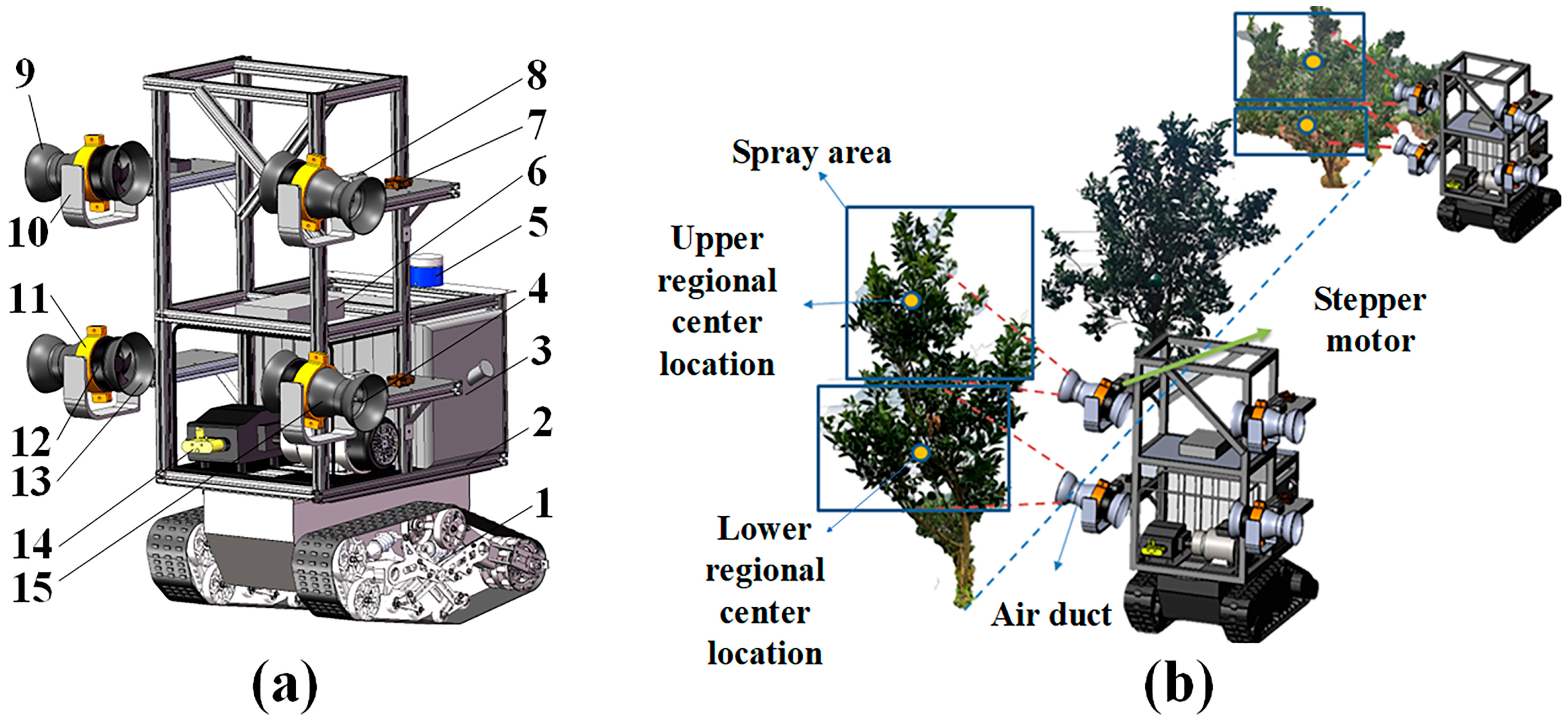
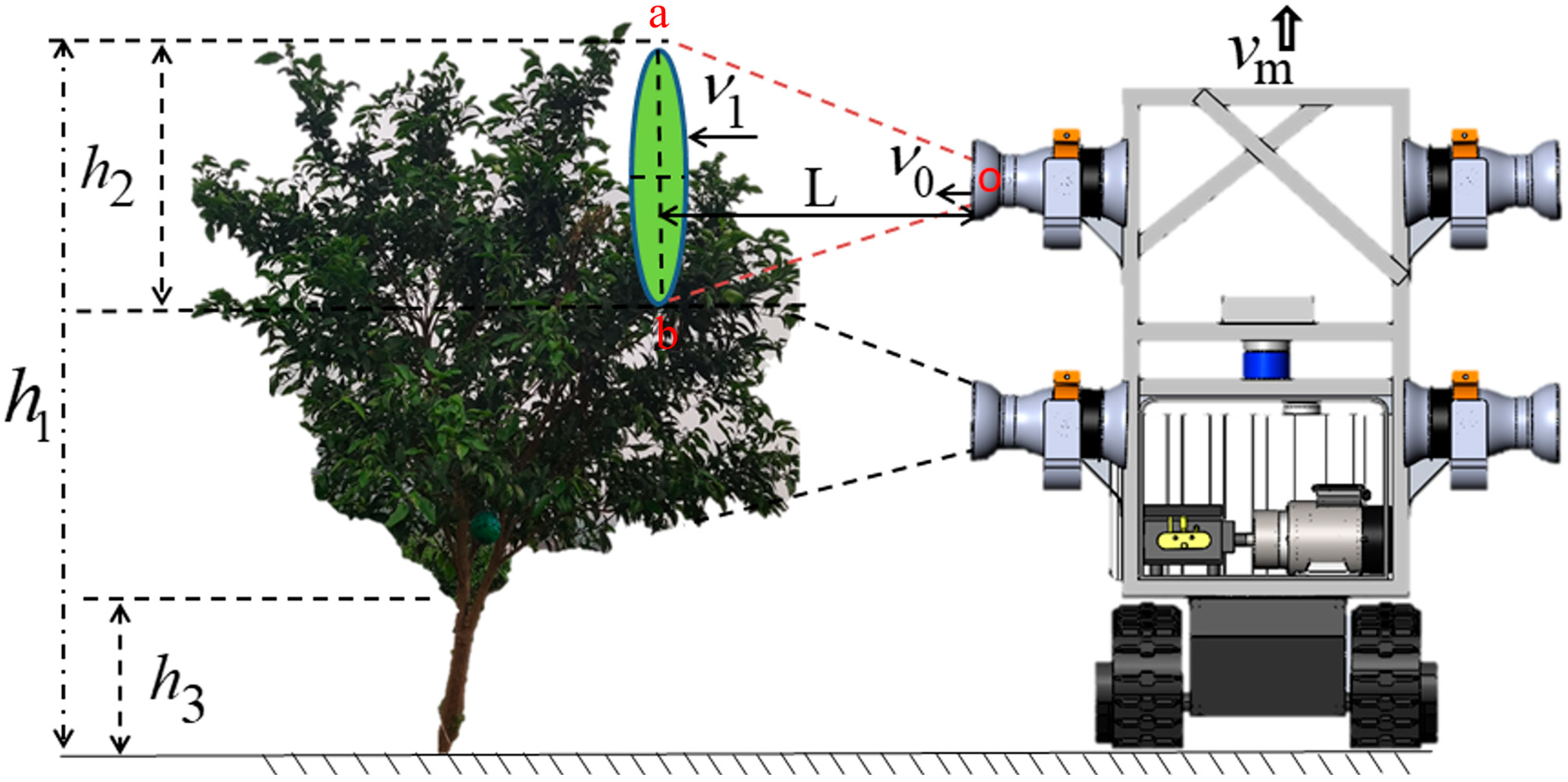
2.1. Overall Structure and Working Principle of the Orchard Sprayer

In hilly citrus orchards, fruit trees typically have a height of 1.5–2.5 m, a crown diameter of 1.0–2.0 m, a row spacing of 3.0–5.0 m, and a plant spacing of 2.5–3.0 m. The air-assisted sprayer was designed using SolidWorks (2020, Dassault Systèmes, Waltham, MA, USA) (Figure 1a). The spraying system consists of a flow collector, an axial fan (6318/2TDH4P, Ebm-papst, Mulfingen, Germany), an air duct, a flare tube, and a rectifier, which are installed at the upper and lower positions on both sides of the machine. The combination of the air duct, flare tube, and rectifier (air-assisted system) enhances the average airflow velocity and uniformity at the outlet of the spraying device. The main technical parameters of the air-assisted system are listed in

Table 1. Main technical parameters of the air-assisted system.

Parameters	Value
End diameter of flare tube (mm)	220
Length of tapering air duct (mm)	190
End diameter of tapering air duct (mm)	125
Maximum diameter of tapering air duct (mm)	170
Diameter of axial fan (mm)	162
Number of axial fan blades (unit)	5
Length of fan casing (mm)	60
Diameter at the air inlet of the flow collector (mm)	220
Length of flow collector (mm)	35
Taper angle of air duct (°)	17

.

2.2. Determination of Axial Fan Parameters

2.2.1. Calculation of Fan Airflow Capacity

The air-assisted sprayer is mounted on a tracked chassis (Komodo-02, JCRobot, Taian, China) and operates between rows in hilly orchards, where droplets are delivered to the target area with the assistance of the axial fan (Figure 1b). Due to the significant variations in tree height, canopy width, and density in citrus orchards, the axial fan is selected for its ability to adjust airflow velocity and volume in real time, ensuring effective droplet transport into the tree canopy. Airflow volume and velocity are key parameters for the sprayer, and the selection of the axial fan must comply with the principles of airflow displacement and terminal airflow velocity [34].

Figure 2 illustrates the airflow displacement schematic. Based on the airflow displacement principle of the sprayer, the airflow generated by the fan must be able to displace the volume of space involved in droplet movement within the triangular cross-sectional area a/b/o shown in Figure 2. Therefore, the required airflow for the sprayer is calculated as follows:

$$Q\ge {\nu }_{m}LK(h_1-h_3)/(2N)$$

(1)

where $Q$ represents the fan airflow capacity, m³/h; ${\nu }_m$ represents the sprayer speed, m/s; $L$ represents the single-side spraying distance, m; $h_3$ represents the canopy height above the ground, m; $N$ represents the number of independent fans, $N$= 2; $h_1$ represents the tree height, ranging from 1.0 to 2.0 m; $K$ represents the airflow loss coefficient along the path, ranging from 1.2 to 1.4.

In this study, the reference tree height is 1.0–2.0 m, with an average canopy diameter of 1.0 m, and $K$ is set to 1.2. The parameter values are as follows:

V_m = 0.5–0.7 m/s, L = 0.6–1.1 m, h₁ = 1.8 m, h₃ = 0.4 m.

Substituting these parameters into the equation, the airflow capacity of a single independent fan is calculated as $Q$ = 453.6–1164.24 m³/h.

2.2.2. Calculation of Fan Outlet Airflow Velocity

According to the terminal airflow velocity principle, the airflow velocity at the outlet is calculated using the following formula:

$$v_0=v_1\left(h_1-h_3\right)/(h_{2}K)$$

(2)

where $v_0$ represents the fan outlet airflow velocity, m/s; $v_1$ represents the terminal airflow velocity upon reaching the canopy, m/s; $h_2$ represents the coverage width of a single fan, m; $h_2$ is taken as 0.6–1.0 m when the spraying distance is 0.6–1.2 m. In this study, the required terminal airflow velocity $v_1$ for citrus trees is set to 9.0 m/s. The calculated fan outlet airflow velocity $v_0$ is 10.5–17.5 m/s.

Additionally, to compensate for dynamic and static pressure losses along the airflow path, the axial fan must provide a certain level of air pressure. The air pressure is calculated using the following formula:

$$\begin{array}{l}\left\{\begin{array}{c}{P}_d={\rho }_a{v}_0^2/2\\ P_m=\psi {\rho }_a{v}_0^{2}l/d\\ P_z=\xi {\rho }_a{v}_0^2/2\end{array}\right.\\ P_{total}=P_d+P_m+P_z\end{array}$$

(3)

where $P_d$, $P_m$, and $P_z$ represent dynamic pressure loss, frictional pressure loss, and local pressure loss, respectively; ${\rho }_a$ is the air density, taken as 1.22 kg/m³; $v_0$ = 17.5 m/s; $\psi$ is the friction factor, taken as 0.1; $d$ is the fan diameter, taken as 0.162 m; $\xi$ is the local resistance coefficient, taken as 0.3; $l$ is the duct length (including the fan casing length), taken as 0.25 m. The calculated minimum air pressure required for a single fan is 300.52 Pa.

Based on the above calculation results, the selected axial fan specifications are shown in

Table 2. Technical parameters of the axial flow fan.

Parameters	Value
Dimensions (mm)	172 × 160 × 51
Power (W)	135
Speed range (r/min)	1000–9000
Operating voltage (V)	32–72 DC
Airflow (m3/s)	0.264
Maximum wind pressure (Pa)	400

.

2.3. Simulation Parameters for the Sprayer Airflow Field

To investigate the impact of different air duct structures on the airflow field of the sprayer, this study utilizes Fluent (2022, ANSYS, Inc., Canonsburg, PA, USA) for CFD numerical simulations. A comparative analysis is conducted on the internal and external flow fields of the air duct with a flare tube and rectifier. Additionally, the effect of the number of guide vanes on airflow distribution is quantified. On this basis, the study also comprehensively examines the effects of fan speed, spray pressure, and spray distance on droplet transport.

2.3.1. Governing Questions and Models

According to the principle of mass conservation, and disregarding the heat transfer and droplet evaporation between the droplets and airflow, as well as other forms of energy transfer during the numerical simulation of the airflow field, the three-dimensional continuity equation for the fluid can be expressed in its differential form as [35]

$${\displaystyle \frac{\partial \rho }{\partial t}}+{\displaystyle \frac{\partial \left(\rho u_x\right)}{\partial x}}+{\displaystyle \frac{\partial \left(\rho u_y\right)}{\partial y}}+{\displaystyle \frac{\partial \left(\rho u_z\right)}{\partial z}}=0$$

(4)

where $\rho$ is the fluid density, kg/m³; $u_x$, $u_y$, $u_z$ are the velocity components in the x, y, and z directions, respectively, m/s; t is time, s.

According to the principle of momentum conservation, the component form of the momentum conservation equation for the fluid is given by:

$$\left\{\begin{array}{l}{\displaystyle \frac{\partial \left(\rho u_x\right)}{\partial t}}+div\left(\rho u_x\overrightarrow{u}\right)=-{\displaystyle \frac{\partial P}{\partial x}}+{\displaystyle \frac{\partial {\tau }_{xx}}{\partial x}}+{\displaystyle \frac{\partial {\tau }_{yx}}{\partial y}}+{\displaystyle \frac{\partial {\tau }_{zx}}{\partial z}}+\rho f_x\\ {\displaystyle \frac{\partial \left(\rho u_y\right)}{\partial t}}+div\left(\rho u_y\overrightarrow{u}\right)=-{\displaystyle \frac{\partial P}{\partial y}}+{\displaystyle \frac{\partial {\tau }_{xy}}{\partial x}}+{\displaystyle \frac{\partial {\tau }_{yy}}{\partial y}}+{\displaystyle \frac{\partial {\tau }_{zy}}{\partial z}}+\rho f_y\\ {\displaystyle \frac{\partial \left(\rho u_z\right)}{\partial t}}+div\left(\rho u_z\overrightarrow{u}\right)=-{\displaystyle \frac{\partial P}{\partial z}}+{\displaystyle \frac{\partial {\tau }_{xz}}{\partial x}}+{\displaystyle \frac{\partial {\tau }_{yz}}{\partial y}}+{\displaystyle \frac{\partial {\tau }_{zz}}{\partial z}}+\rho f_z\end{array}\right.$$

(5)

where $P$ is the static pressure on the fluid particle, Pa; ${\tau }_{ij}$ (where i takes values of x, y, z, and j also takes x, y, z, respectively) are the components of the viscous stress $\tau$ acting on the surface of the fluid particle; $f_i$ represents the unit mass force components acting on the fluid particle in the x, y, and z directions, m/s²; $\rho f_i$ represents the body force components in the x, y, and z directions on the fluid particle.

The turbulent characteristics of the gas phase are described using the RNG (Renormalization-Group) $k$-$\epsilon$ turbulence model [36], while droplet motion is simulated using the DPM (Discrete Phase Model). The calculations are performed using the SIMPLE algorithm for pressure–velocity coupling, with the pressure term discretized using a second-order scheme.

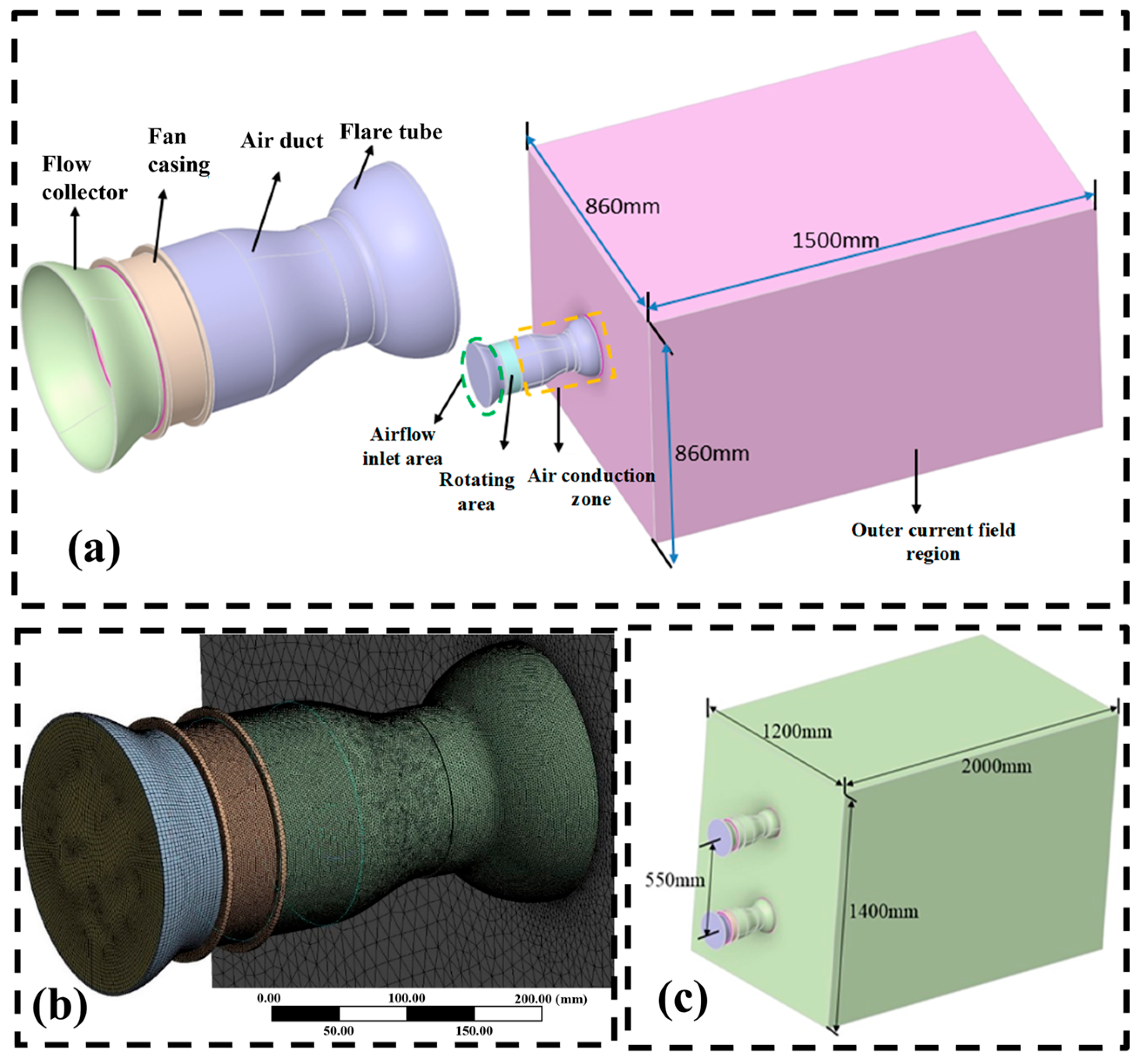
2.3.2. Computational Domain and Boundary Conditions

The airflow domain model for the sprayer is established using SolidWorks (2020, Dassault Systèmes, Waltham, MA, USA), with a focus on analyzing the impact of the absence of an air duct and different air duct shapes on the fan’s flow field. The three-dimensional model includes the airflow inlet zone, the rotating zone, the airflow guiding zone, and the external flow field zone, where the dimensions of the external flow field are set to 860 mm × 860 mm × 1500 mm. To improve the efficiency of the simulation calculations, the model simplifies structures such as the chassis, frame, and connectors. Using the air duct with a flare tube as an example, the final fluid domain model of the axial fan is shown in Figure 3a, and the modeling approach for other air duct configurations is the same.

The overall flow field employs a tetrahedral unstructured mesh. Since the local mesh count varies with the shape of the air duct, a grid independence verification was conducted by setting global mesh sizes of 0.015 m, 0.020 m, 0.025 m, 0.030 m, 0.035 m, and 0.040 m, and comparing the outlet flow rate results for each configuration. To balance computational accuracy and resource consumption, the global mesh size is set to 0.03 m. Local mesh refinement is applied based on different region characteristics: the inlet region is set to 0.005 m, the fan blade region is refined to 0.002 m, and the air duct fluid domain is set to 0.003 m. Three boundary layers are added in key flow regions to improve computational accuracy. The mesh size for the external flow field domain is set to 0.020 m. Mesh quality is evaluated using orthogonal quality and skewness metrics. The statistical results indicate that the minimum orthogonal quality is greater than 0.01, the maximum skewness is 0.80, and the average skewness is 0.19, meeting the quality requirements. The mesh division for the wind-assisted spraying model follows the optimized air duct configuration while neglecting the fan casing and flow collector structures to reduce computational cost.

Using the air duct with a flare tube as an example, the local mesh division is shown in Figure 3b. The sliding mesh method is employed to simulate the rotating region of the fan. The inlet and outlet boundary conditions are set as the pressure inlet and pressure outlet, respectively, with interface matching used for data exchange at the interfaces. The fluid–solid interface is defined as a coupled wall, and fluid region interfaces are set as matching, while other walls maintain the default no-slip boundary condition.

A coupled flow field model of airflow and droplets is established for the single-sided sprayer to study its spatial motion characteristics. The single-sided setup includes two air duct structures: an integrated air duct at the top and an independently installed air duct at the bottom, with a center spacing of 550 mm. The external flow field dimensions are set to 2000 mm × 1200 mm × 1400 mm (Figure 3c).

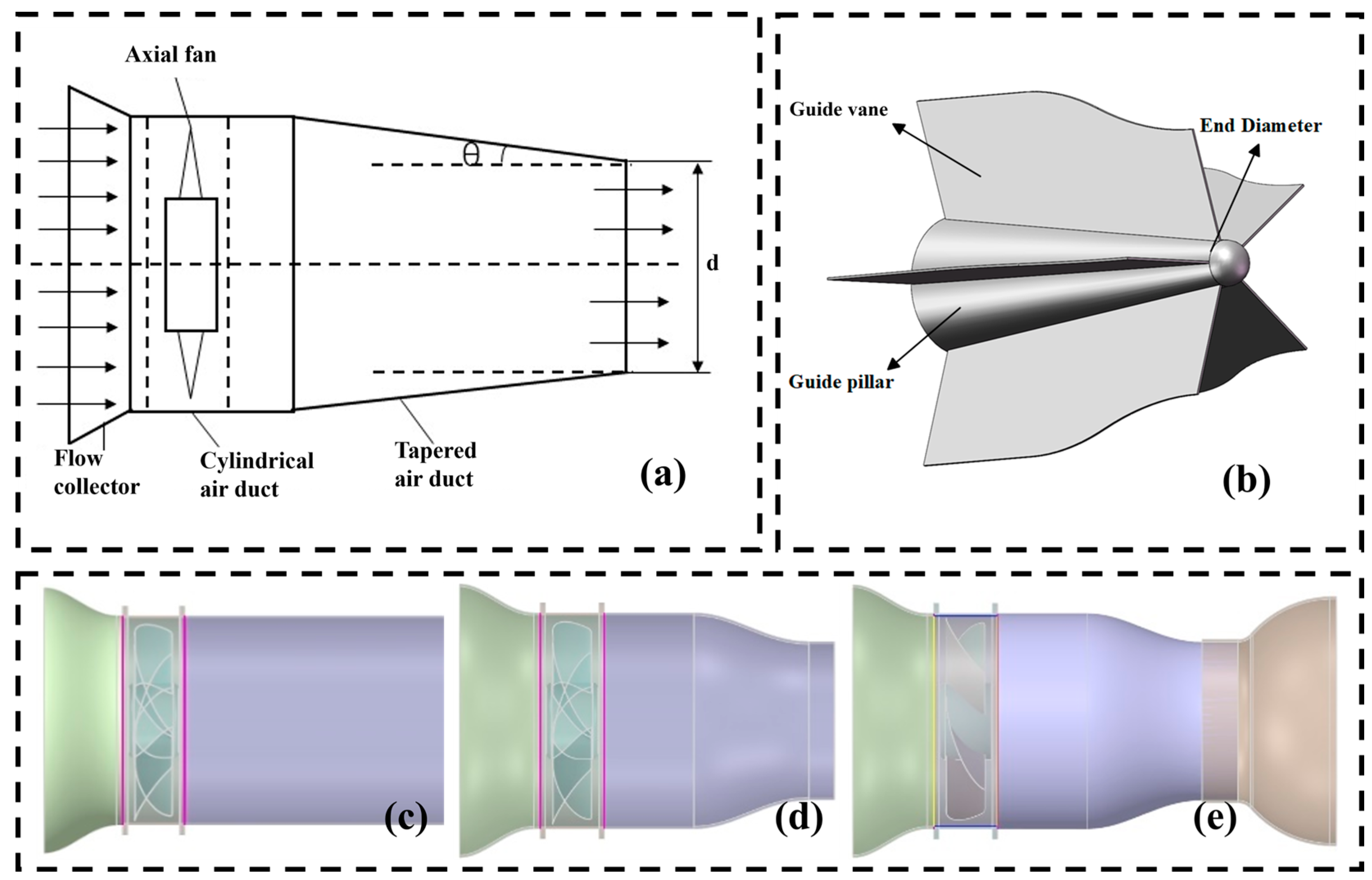
2.3.3. Model Construction of the Air Duct and Rectifier

The air duct is primarily used to guide the airflow from the axial fan in a predetermined direction while maintaining a high axial velocity. This optimizes the airflow distribution and enhances droplet transport efficiency, thereby improving the uniformity of spray deposition. In this study, three air duct structures—constant-diameter type, converging type, and flare tube-equipped type—were selected. Along with a no-air duct configuration, numerical simulations were conducted to compare their spray airflow characteristics and determine the optimal structure.

Although the air duct can expand the airflow distribution range, adding a flare tube may reduce the uniformity of the external flow field and increase turbulence, which is unfavorable for directional droplet transport. To optimize airflow direction and minimize kinetic energy loss caused by turbulence, a rectifier was installed inside the air duct. The number of guide vanes significantly affects airflow direction and distribution [37]. To enhance rectification performance, CFD simulations were conducted for rectifier with 2 to 7 blades to determine the optimal blade count. The three-dimensional structures of various air ducts and rectifiers are shown in Figure 4.

2.4. Air Speed Verification and Boundary Measurement

To verify the accuracy of the simulation boundary conditions, a bench test was conducted to validate the air speed and airflow field distribution of the air duct system, as shown in Figure 5a.

The experimental setup consists of a spray-assisted airflow system and an airflow measurement system. A split-type anemometer (AS-H, Aicevoos, Wuhan, China) was used to measure air speed, with the axial fan speed set at 5000 r/min. The temperature and humidity were measured with a thermometer-hygrometer (TH101B, Anymetre, Guangzhou, China) at 13 °C ±1 °C and 75% ± 5%, respectively. Tap water was used as the test medium.

The airflow velocity measurement method is defined as follows: The horizontal airflow transport direction is set as the Z-axis, the vertical upward direction as the positive Y-axis, and the X-axis positive direction is perpendicular to the YZ plane, pointing to the right. Taking the spray air outlet plane as the reference, measurement lines were arranged at five positions: upper, middle, lower, left, and right. Measurement points were set along the Z-axis at 0.1 m, 0.3 m, 0.5 m, 0.7 m, 0.9 m, and 1.1 m to construct the measurement plane. Finally, the measured air speed along the central axis was compared with the simulation results. The schematic diagram of the measurement points is shown in Figure 5b.

To determine the axial air speed boundary of the axial fan, nine measurement planes were set at distances of 0 m, 0.1 m, 0.3 m, 0.5 m, 0.7 m, 0.9 m, 1.1 m, 1.3 m, and 1.5 m from the air outlet. On each plane, the anemometer was adjusted to move along four reference lines (upper, lower, left, and right) to measure the air speed distribution. The position where the air speed dropped to 1.5 m/s was identified as the air speed boundary, and its distance from the central axis was measured and recorded using a tape measure.

In the air speed validation experiment, after the spray-assisted airflow system stabilized, the anemometer was placed at the designated measurement points, ensuring that its impeller axis was aligned with the airflow direction. Air speed at each measurement point was recorded three times, and the average value was taken as the final result.

During the experiment, two installation methods were used for the flare tube and air duct: integrated installation and independent installation. In the integrated installation, the flare tube and air duct were designed as a single unit, which moderately expanded the airflow range while reducing axial air speed, thereby decreasing droplet drift at the top of the canopy. In the independent installation, the separate flare tube was fixed to the end of the air duct, resulting in a more concentrated and higher air speed. The integrated flare tube and air duct were placed above the sprayer to minimize droplet drift beyond the upper canopy, while the independently installed flare tube was positioned below the sprayer to enhance penetration through the lower canopy, enabling differential airflow delivery based on actual canopy characteristics.

2.5. Simulation Experiment

2.5.1. Optimization of Air-Assisted Spraying Components Simulation

The simulations are conducted to analyze the flow field distribution of the selected axial fan, considering different air-assisted configurations: no air duct, uniform diameter air duct, converging air duct, and converging air duct with a flare tube. The impact of different air duct types and flare tubes on the airflow is discussed.

To facilitate the generation of directional airflow by the air duct and reduce the kinetic energy loss caused by turbulence, a flow rectifier is added inside the air duct. The number of blades in the rectifier will affect the axial velocity of the airflow. The number of blades is set to 2, 3, 4, 5, 6, and 7, and three-dimensional models are constructed for simulation analysis.

2.5.2. Air-Assisted Spray Flow Field Pattern Experiment

To study the effects of axial fan speed, spray pressure, and spray distance on droplet transport, the axial fan speed is set between 2000–7000 r/min, the spray pressure ranges from 0.4–1.0 MPa, and the spray distance is set based on the tree row spacing, ranging from 0.7 to 1.2 m. Simulations and analyses were conducted sequentially for the three factors mentioned above to determine the optimal experimental parameters. The experimental conditions and variable values for each simulation experiment are shown in

Table 3. Experimental conditions and values of variables for simulation experiments.

	(1) Fan Speed	(2) Spray Pressure	(3) Spray Distance
Condition	Spray pressure = 0.4 MPa Spray distance = 0.9 m	Fan speed = 4000 r/min Spray distance = 0.9 m	Fan speed = 4000 r/min Spray pressure = 0.6 MPa
Value	{2000, 3000, 4000, 5000, 6000, 7000}/(r/min)	{0.4, 0.6, 0.8, 1.0}/(MPa)	{0.7, 0.8, 0.9, 1.0, 1.1, 1.2}/(m)

. The results and discussion of the simulation experiments are presented in Section 3.4–Section 3.6.

(1)

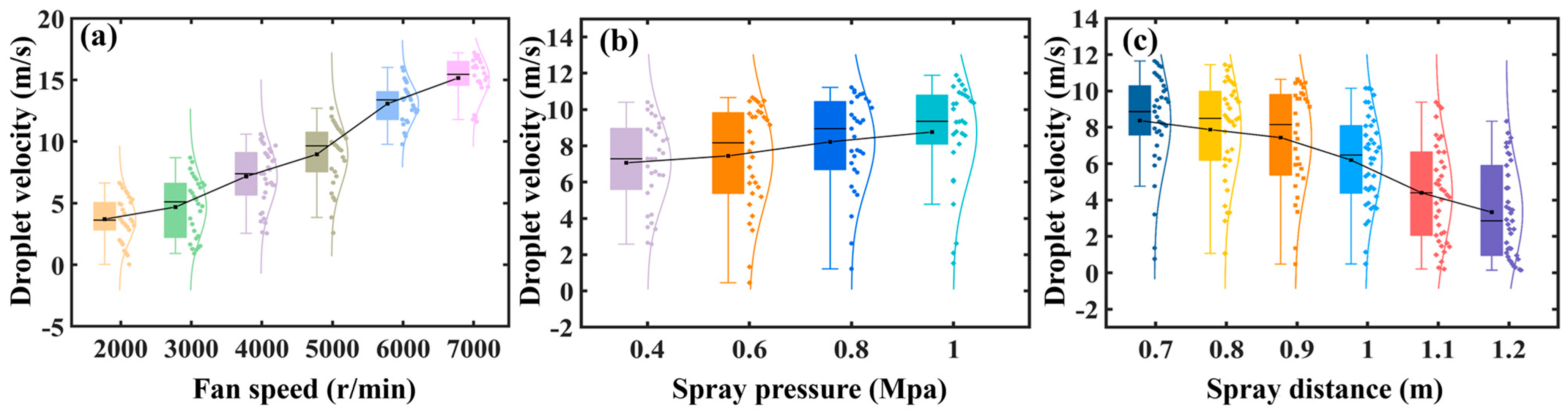
Effect of different fan speed on droplet movement. Set the spray pressure to 0.4 MPa and the spray distance to 0.9 m to investigate the droplet deposition characteristics at axial fan speeds of 2000 r/min, 3000 r/min, 4000 r/min, 5000 r/min, 6000 r/min, and 7000 r/min.

(2)

Effect of different spray pressure on droplet movement. Set the axial fan speed to 4000 r/min and the spray distance to 0.9 m to investigate the droplet deposition characteristics at spray pressures of 0.4 MPa, 0.6 MPa, 0.8 MPa, and 1.0 MPa.

(3)

Effect of different spray distance on droplet movement. Set the axial fan speed to 4000 r/min and the spray pressure to 0.6 MPa to investigate the droplet deposition characteristics in the vertical plane at spray distances of 0.7 m, 0.8 m, 0.9 m, 1.0 m, 1.1 m, and 1.2 m.

2.6. Evaluation of Droplet Deposition

To evaluate droplet deposition, droplets were sampled on the corresponding spray distance plane and regarded as the effective deposition amount. The deposition area was defined as the primary deposition surface B, formed by the intersection of the nozzle spray angle and the central axis on the sampling plane, with a radius denoted as $R_p$, as shown in Figure 6.

Thus, the droplet deposition on the sampling plane can be calculated using the following equation:

$$\left\{\begin{array}{c}{V}_p={\displaystyle \frac{4}{3}}\pi {\left({\displaystyle \frac{{\overline{d}}_p}{2}}\right)}^3\\ B=\pi {\left(L\tan {\theta }_1\right)}^2\\ Y_n={\displaystyle \frac{{\rho }_p{V}_p{I}_p}{2B}}\end{array}\right.$$

(6)

where $Y_n$ is the droplet deposition amount, µL·cm⁻²; $L$ represents the spray distance, cm; $B$ represents the area of the sampling plane, cm²; ${\rho }_p$ represents the concentration of the spray solution, L/m³; ${\overline{d}}_p$ is the average droplet diameter in the sample, µm; $V_p$ represents the average volume of the sampled droplets, µm³; $I_p$ is the total number of sampled droplets, and ${\theta }_1$ is the spray half-angle, °.

3. Results and Discussion

3.1. Air Speed Verification and Analysis

The comparison between the measured axial air speed values and the simulated values along the centerline in the 0–1.1 m region is shown in

Table 4. Distribution of air speeds at specified distances for the two mounted methods.

Mounted	Distance from Air Outlet (m)	Air Velocity (m/s)			Results		Relative Error (%)
		I	II	III	Average (m/s)	Simulation (m/s)
Integrated	0.1	15.07	15.05	15.06	15.06	13.16	14.44%
	0.3	14.22	14.25	14.22	14.23	14.95	−4.82%
	0.5	13.08	13.08	13.05	13.07	14.48	−9.74%
	0.7	11.46	11.44	11.45	11.45	13.69	−16.36%
	0.9	10.65	10.63	10.61	10.63	12.96	−17.98%
	1.1	9.78	9.77	9.79	9.78	12.23	−20.03%
Independent	0.1	16.34	16.35	16.33	16.34	15.57	4.95%
	0.3	16.03	16.07	16.04	16.05	16.94	−5.27%
	0.5	15.01	15.03	15.02	15.02	16.18	−7.17%
	0.7	13.23	13.27	13.29	13.26	15.87	−16.43%
	0.9	12.16	12.19	12.18	12.18	14.92	−18.39%
	1.1	10.09	10.06	10.07	10.07	12.58	−19.93%

.

Based on the centerline air speed measurement results, as the spray distance increases, the airflow velocity decreases rapidly. When the spray distance is 0.1 m, the measured value is higher than the simulated value, and the error is relatively large. This discrepancy is primarily due to the presence of strong turbulence at the outlet of the axial fan when operating at high rotational speeds, which leads to fluctuations and instability in the airflow velocity. In addition, the fan outlet is a region of complex flow development where transient eddies and local acceleration or deceleration of the flow may occur, resulting in higher instantaneous velocity peaks that are captured by experimental measurements but not fully represented in steady-state simulation results [38]. When the spray distance is equal to or greater than 0.3 m, the measured value is lower than the simulated value, and the error increases with the distance, but the overall relative error remains within 21%, it is acceptable in orchard and fruit tree crop protection applications [24,39]. The centerline air speed is relatively stable, showing a gradient decrease, and at a spray distance of 1.1 m, the airflow final velocity still meets the required standard.

On the basis of measuring the centerline air speed, the air speed boundary at the upper and lower ends of the axial fan is further determined by measuring the air speed boundary values on the plane 0.1–1.5 m from the air outlet. By adjusting the position of the anemometer, when the measured value is 1.5 m/s, the air speed boundary on the plane is determined. The distance is measured and recorded using a ruler. Four points are measured on each plane (up, down, left, and right), with each point measured three times and the average value taken. The measurement results are shown in Figure 7a,b.

According to the measured results of the effective air speed boundary, the effective air speed boundaries of the upper and lower air ducts are approximately symmetrical in both the vertical and horizontal planes. The overall air duct effective boundary shows a linear expansion trend, while the effective boundary of the independently installed air duct exhibits a curved expansion trend. The difference may stem from the shape of the flare tube outlet and measurement errors. As the distance increases, the boundary increment decreases, indicating that the axial fan has a high airflow concentration, which helps maintain the circular jet form and prevents droplet drift. When the spray distance is 1.1 m, the effective air speed boundaries of the upper and lower air ducts tend to converge, with a small difference. The maximum effective boundary of the integrated air duct in the horizontal plane is 18.4 cm, and in the vertical plane is 18.1 cm; for the independently installed air duct, the maximum effective boundary in the horizontal plane is 17.2 cm, and in the vertical plane is 17.0 cm, providing a reference for the spatial arrangement of the air ducts.

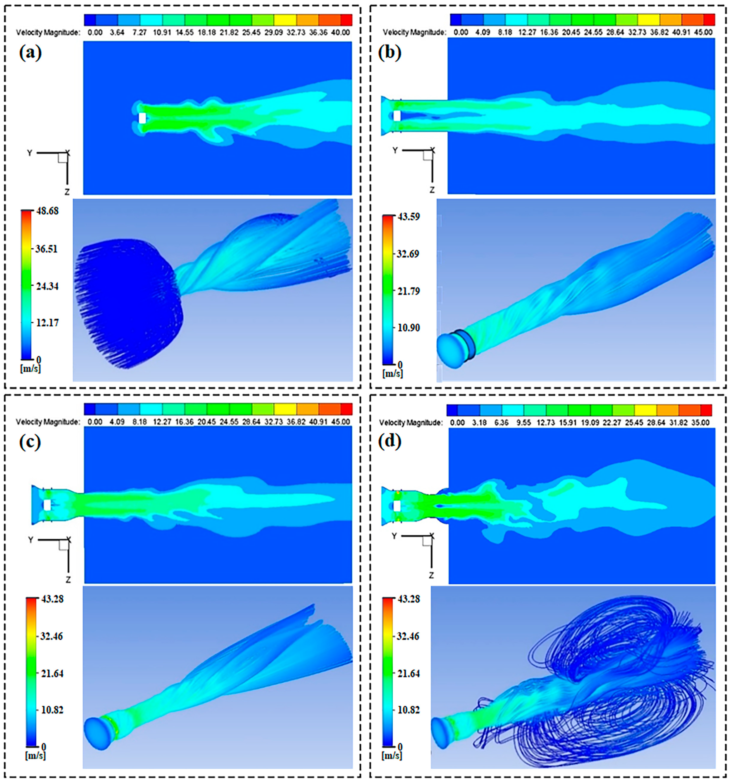
3.2. The Impact of the Air Duct on the Flow Field

Based on the presence or absence and shape differences of the air duct, the flow field distribution of the selected axial fan was simulated, resulting in the flow field distribution and wind field streamline velocity, as shown in Figure 8.

When the air speed is 9 m/s and there is no air duct, only a small amount of turbulence forms in the outflow field, and the air speed of 9 m/s starts to decay at a distance of 0.86 m from the outlet. After installing the converging tube, the range of the 9 m/s air speed increased by 15.12% and 9.30%, compared to no air duct and the constant-diameter tube, respectively. A air speed of 1.5 m/s was used as the threshold for effective airflow coverage, as lower speeds weaken the airflow’s droplet-carrying capacity and reduce canopy penetration. After incorporating the flare tube, the effective airflow coverage area at 0.7 m from the outlet reached 0.071 m², which is an increase of 20.34% and 31.48% compared to the constant-diameter tube and converging tube, respectively. However, severe turbulence still exists in the outflow field.

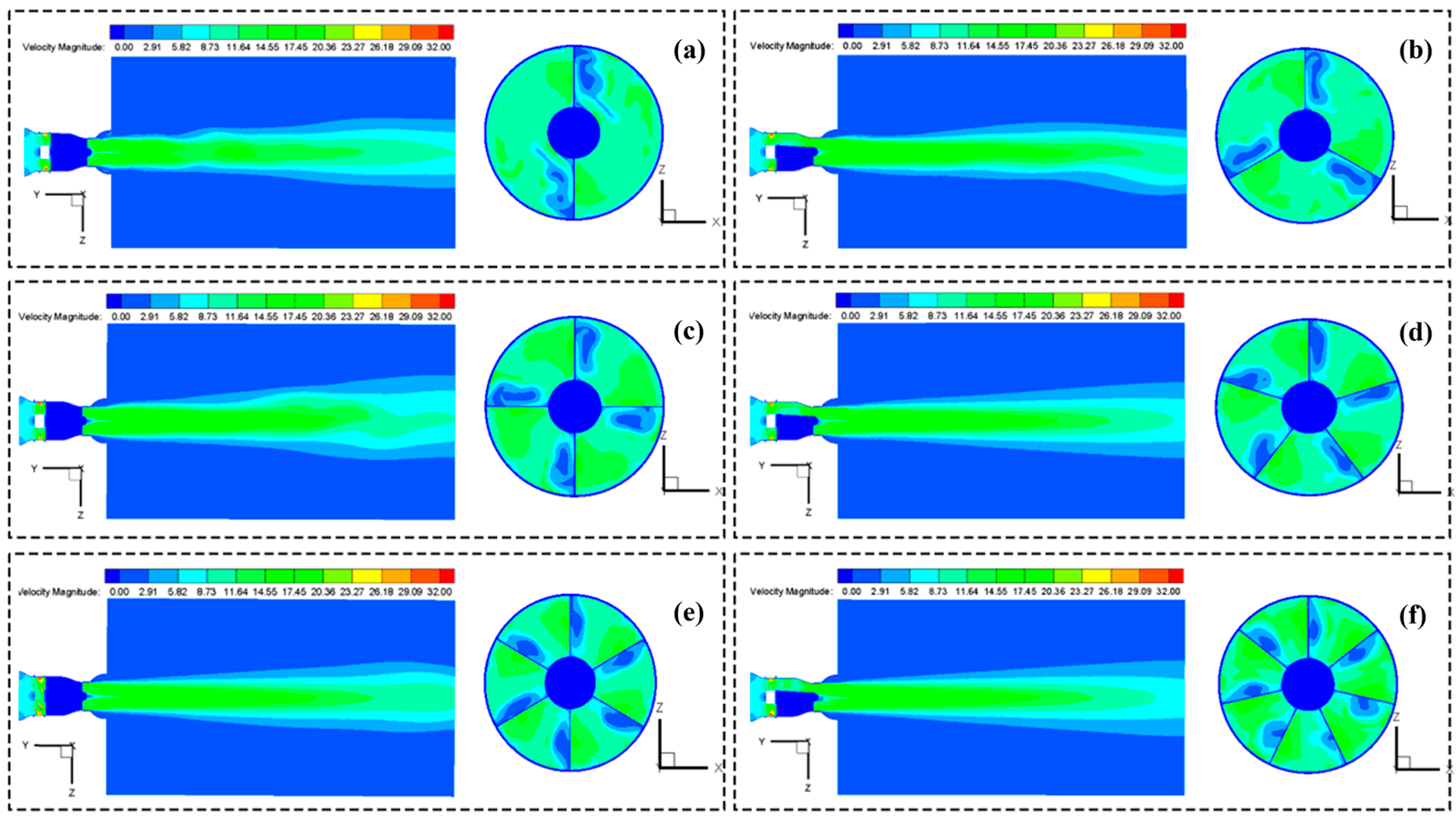
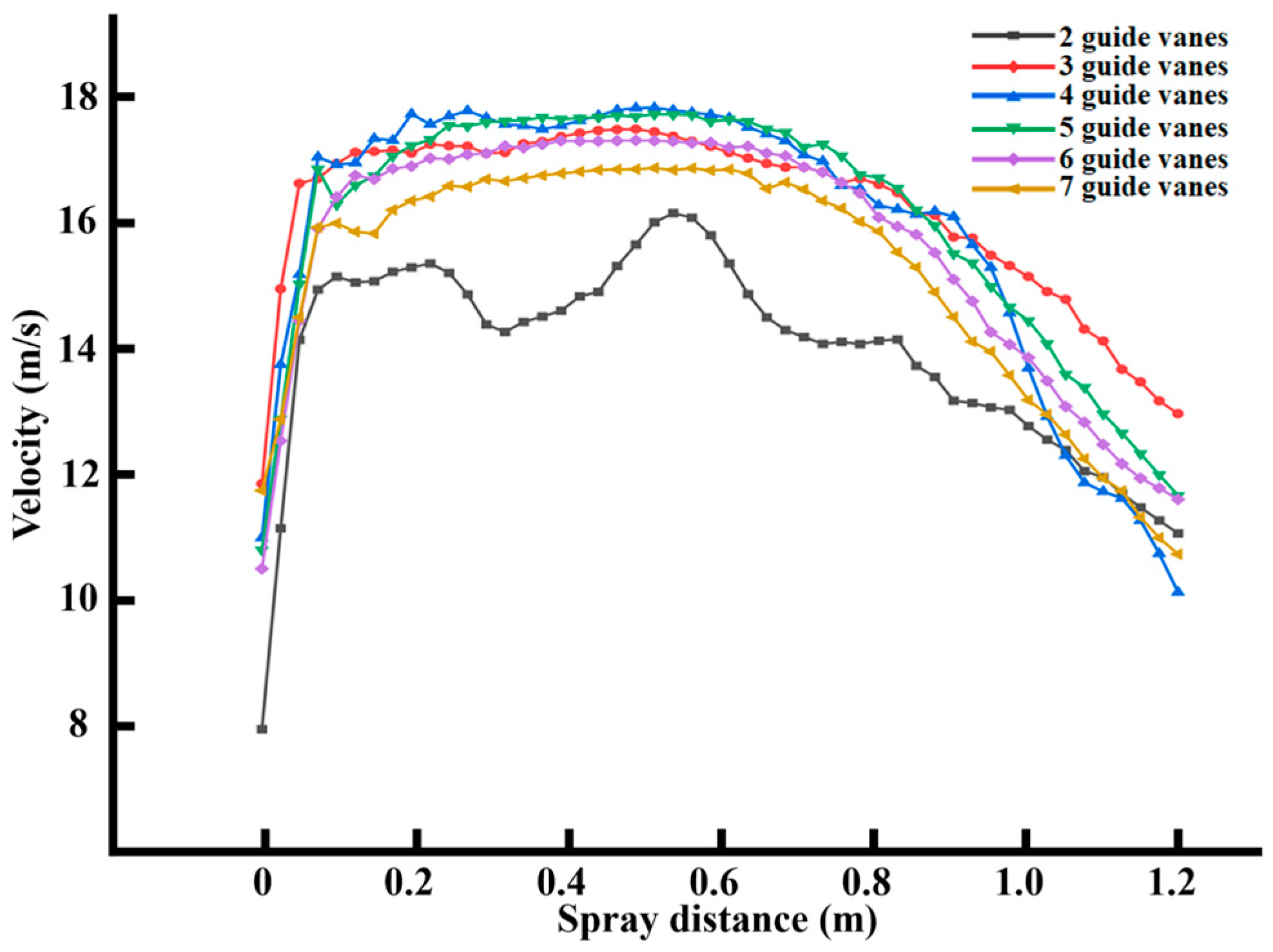
3.3. The Impact of the Number of Guide Vanes on the Flow Field

To determine the optimal number of guide vanes, simulations were conducted to analyze the effects of different numbers of guide vanes, ranging from two to seven blades. The velocity contour maps of the flow field inside and outside the air duct, as well as the velocity distribution of the internal flow field, were obtained, as shown in Figure 9. The airflow coverage area on planes 0.2 to 1.2 m from the outlet was analyzed to determine the effective airflow coverage area corresponding to different numbers of guide vanes on each plane (Figure 10).

When the number of guide vanes is between two and four, the internal flow field has a larger turbulence area, and the external flow field exhibits turbulence and rotational airflow (Figure 9a–c). Although the guide vanes in the air duct are fixed structures arranged in an axially symmetrical manner, the turbulence shown in the figure is predominantly concentrated on one side of the vanes, exhibiting a distinctly asymmetric flow pattern. Possible reasons for this phenomenon include the residual rotational momentum of the helical airflow generated by the rotating fan, which is retained as it enters the air duct. Upon encountering the fixed guide vanes, this rotational flow is disrupted, leading to a redistribution of velocity wherein a high-speed region forms on the windward side and a low-speed region on the leeward side, thereby inducing asymmetric turbulent structures [40].

As the number of guide vanes increases, the axial velocity at the airflow outlet tends to stabilize, and the radial distribution becomes more uniform in a gradient. When the number of guide vanes is odd, the uniformity and symmetry of the airflow distribution in the external flow field are better compared to even-numbered vanes, leading to improved airflow stability with a symmetrical distribution both vertically and horizontally (Figure 9d,f). This phenomenon can be attributed to the spatial interference characteristics introduced by the arrangement of guide vanes. When the number of guide vanes is even, diametrically opposed vanes tend to form symmetric interference pathways, which promote the formation of strong recirculation zones and shear layers along specific radial directions. These flow interactions often result in localized turbulence enhancement and reduce the overall symmetry of the external airflow field. In contrast, an odd number of guide vanes disrupts this radial symmetry, preventing the formation of directly opposing vane pairs. This irregular spacing reduces coherent flow interference patterns and disperses vortex shedding events more evenly around the circumference. As a result, the airflow downstream exhibits lower anisotropy, with improved uniformity and symmetry in both the vertical and horizontal directions. This effect enhances overall flow stability and mitigates the formation of dominant directional disturbances. These observations are consistent with Figure 9d,f, where the external flow fields associated with odd-numbered vanes display a more continuous and symmetric velocity distribution compared to their even-numbered counterparts.

The change in the number of guide vanes has little effect on the effective airflow coverage area, but as the number of guide vanes increases, the distribution of the effective airflow coverage area across different planes becomes more uniform, and turbulence decreases (see Figure 10). In the region from 0 to 0.2 m from the outlet, the airflow from the rectifier’s upper and lower parts converges, causing air speed fluctuations; in the 0.2 to 0.6 m region, a stable high-speed airflow zone exists with a air speed of about 16 m/s, which then rapidly decreases.

Based on the velocity contour maps of the external flow field for each air duct configuration, the velocity attenuation pattern along the central axis was extracted, and the velocity attenuation curve was plotted (Figure 11).

The significant velocity fluctuation observed in the configuration with two guide vanes along the central axis, as shown in Figure 11, can be attributed to insufficient flow constraint and poor azimuthal flow stability caused by the minimal vane count. With only two vanes positioned opposite each other, the airflow experiences strong bidirectional interference, forming recirculation zones and unstable shear layers near the central axis. This limited structural guidance fails to effectively suppress circumferential vortex formation or redirect high-speed airflow symmetrically. Consequently, the central core of the jet becomes highly sensitive to small asymmetries in inlet conditions or numerical disturbances, leading to unsteady velocity peaks and troughs along the spray axis. In contrast, configurations with three or more guide vanes introduce multi-directional flow division and stabilization, effectively smoothing the velocity profile and enhancing axial coherence. As the spraying distance increases, the air speed along the central axis first rises and then decreases. Meanwhile, as the number of guide vanes increases, the effect of the rectifier is enhanced, leading to more stable air speed variations and an increase in the maximum air speed to approximately 18 m/s (with four or five guide vanes). However, an excessive number of guide vanes can obstruct airflow, causing a slight decrease in air speed (with six or seven guide vanes). The results indicate that a rectifier with five blades exhibits good flow-guiding performance, provides a uniform air speed distribution, and maintains a relatively high air speed, meeting the spraying operation requirements of small jet air duct devices.

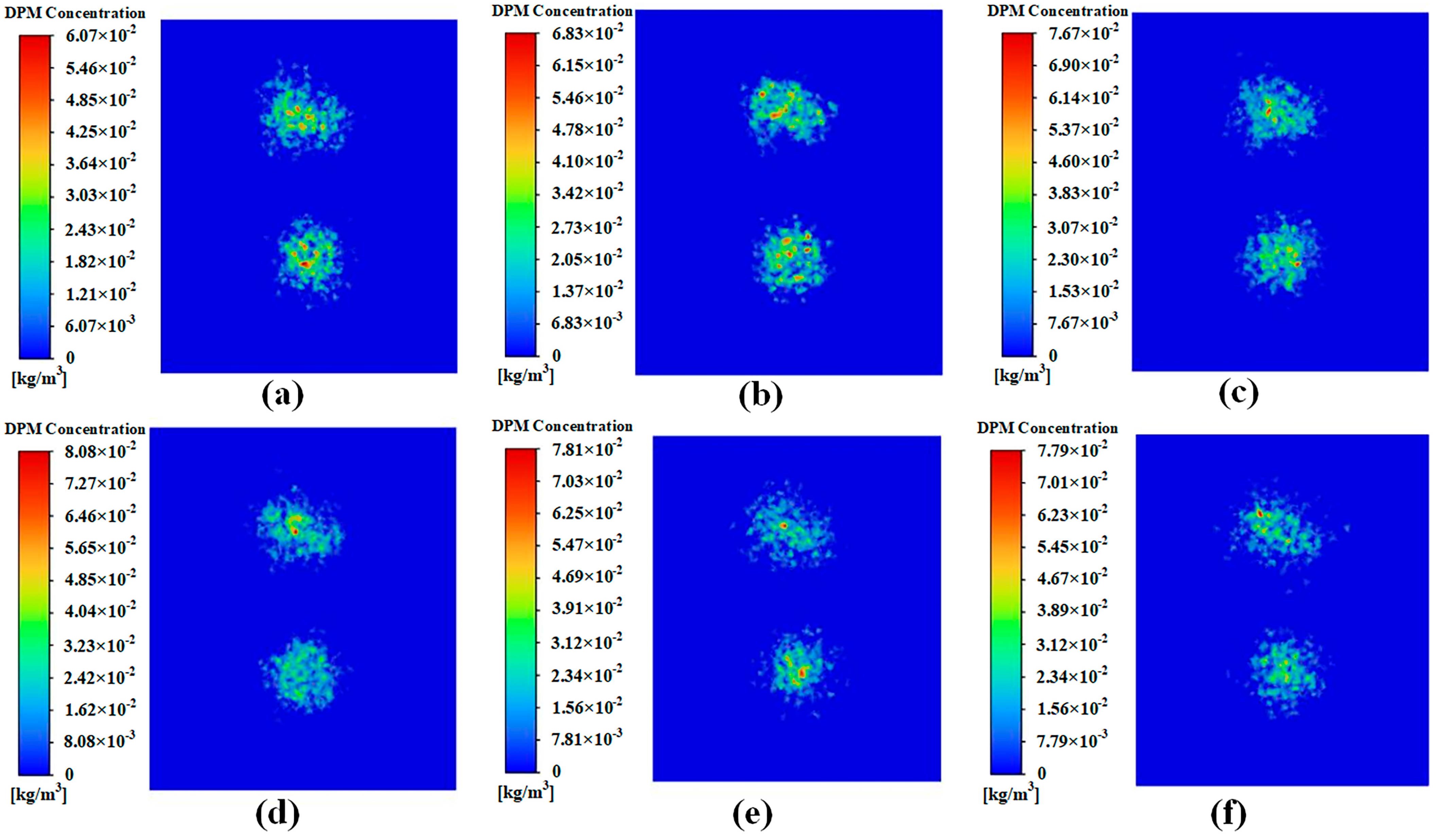
3.4. Effect of Different Fan Speed on Droplet Movement

The simulation results (Figure 12) show the movement and distribution of droplets at different fan speeds.

When the fan speed is 2000 r/min, the droplet transport capability is poor, causing a large number of droplets to detach from the airflow field and disperse. When the fan speed reaches 7000 r/min, turbulence occurs above the air duct, leading to irregular droplet movement along with the turbulent flow. As the fan speed increases from 3000 r/min to 6000 r/min, the diffusion range of the air–liquid jet gradually decreases, improving spraying precision and increasing the spraying range. However, excessively high air velocities (more than 20 m/s) may cause droplets to rebound off leaf surfaces, reducing deposition efficiency. Studies have shown that when the droplet impact velocity exceeds a certain range, especially for droplets with diameters smaller than 100 μm, the likelihood of rebound increases significantly due to insufficient dissipation of kinetic energy during impact [41]. This rebound phenomenon is closely related to the Weber number ($We$), which quantifies the balance between the inertial forces and surface tension of the droplet.

The velocity of different air–liquid mixtures ultimately affects droplet deposition (see

Table 5. Droplet deposition at different fan speeds.

Fan speed (r/min)	2000	3000	4000	5000	6000	7000
Droplet deposition (µL·cm−2)	0.96	1.92	3.72	2.96	1.45	0.87

).

As the fan speed increases, droplet deposition on the plane 0.9 m from the nozzle initially increases and then decreases. When the fan speed is between 3000 and 5000 r/min, droplet deposition reaches a relatively high level, with average droplet velocity (ADV) maintained between 4–9 m/s. When the speed exceeds 6000 r/min, a large number of droplets continue to move forward, resulting in a decrease in droplet deposition.

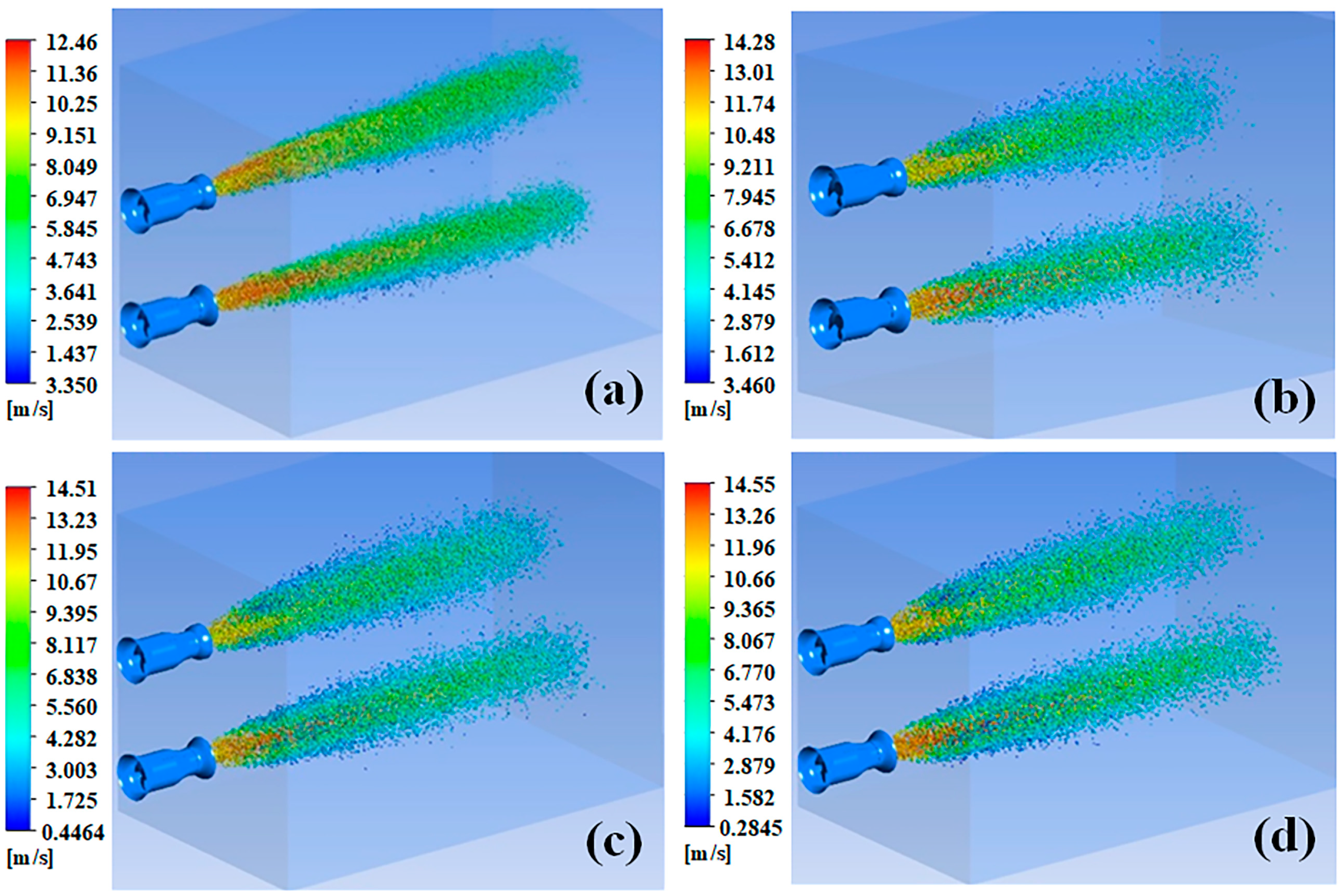
3.5. Effect of Different Spray Pressure on Droplet Movement

The simulation results show the spatial distribution of droplets under different spray pressures, as shown in Figure 13.

When the fan speed is 4000 r/min, for each 0.2 MPa increase in spray pressure from a single nozzle, the droplet diffusion range initially increases and then stabilizes. At a spray pressure of 0.4 MPa, the initial droplet velocity is small, and the airflow exerts a strong constraint on the droplets in the horizontal direction, resulting in a narrower diffusion range. As the spray pressure increases, the velocity of the droplets along the spray angle direction increases, allowing them to maintain this directional motion over a longer distance. When the spray pressure reaches 1.0 MPa, the droplets exhibit a relatively uniform spatial distribution with a wider spray angle and sustained particle velocity near the nozzle outlet, indicating enhanced atomization and dispersion.

Table 6. Droplet deposition at different spray pressures.

Spray pressure (MPa)	0.4	0.6	0.8	1.0
Droplet deposition (µL·cm−2)	3.72	5.11	4.03	3.47

shows the droplet deposition at different spray pressures.

Under constant fan speed and spray distance, droplet deposition increases and then decreases with increasing spray pressure. The highest droplet count proportion occurs at a spray pressure of 0.6 MPa, after which it gradually decreases.

3.6. Effect of Different Spray Distance on Droplet Movement

The previous two sections have provided a detailed analysis of droplet spatial distribution. Therefore, this section uses droplet deposition concentration to evaluate the effect of spray distance on deposition performance, as shown in Figure 14.

As the spray distance increases, the droplet deposition mass concentration on each vertical plane shows a trend of initial increase followed by a slight decrease. Specifically, when the spray distance is between 0.7 m and 1.0 m, the deposition regions are relatively concentrated with higher peak concentrations. At 1.1 m, the highest overall concentration is observed, suggesting optimal coverage. Beyond 1.1 m, such as at 1.2 m, the droplet distribution becomes more scattered, and the peak deposition concentration decreases slightly. This suggests that excessive spray distance leads to wider diffusion and partial droplet sedimentation. While the upper deposition area tends to shift downward with increasing distance, the lower region remains more circular and stable, aligning with the spatial structure of a two-layer canopy.

Table 7. Droplet deposition at different spray distances.

Distance from air outlet (m)	0.7	0.8	0.9	1.0	1.1	1.2
Droplet deposition (µL·cm−2)	2.75	3.77	5.23	4.59	2.51	1.86

shows the droplet deposition at different spray distance planes.

Under constant fan speed and spray pressure, the droplet deposition increases first and then decreases with the spray distance. The droplet number proportion is the highest when the spray distance is between 0.9 to 1.0 m and gradually decreases afterward.

After droplets enter the airflow field, they move in coordination with the airflow, and their speeds tend to align. The distribution of droplet group velocity (DGV) on the plane is organized based on the DGV information, as shown in Figure 15.

When the spray pressure and spray distance are constant, and the fan speed is less than 3000 r/min, the lower quartile of DGV shifts, with the overall speed being smaller and more dispersed. When the fan speed exceeds 3000 r/min, the median droplet velocity (MDV) approaches the center of the box and is higher than the ADV. After the fan speed exceeds 3000 r/min, the DGV distribution becomes more symmetric, and the degree of dispersion decreases. The ADVs at different fan speeds are as follows: 3.62 m/s at 2000 r/min, 4.58 m/s at 3000 r/min, 7.00 m/s at 4000 r/min, 8.76 m/s at 5000 r/min, 12.79 m/s at 6000 r/min, and 14.82 m/s at 7000 r/min. When the fan speed exceeds 6000 r/min, the airflow transport capacity is significantly enhanced, with the DGV exceeding 10 m/s. Droplet rebound may occur when the droplets collide with the leaf surface, causing the droplets to be lost to the ground [42]. However, the velocity gradient remains relatively uniform and follows a normal distribution, further indicating that the droplets are more effectively transported with the airflow, making them less likely to drift during transport and maintaining a certain degree of penetration (Figure 15a).

When the fan speed and spray distance are constant, spray pressure below 1 MPa has little effect on the DGV (Figure 15b). When the spray pressure is ≤0.8 MPa, the droplets are gradually entrained by the airflow and move according to the airflow distribution pattern, forming a uniform velocity distribution. The DGV is concentrated near the median and remains between 5 and 11 m/s. At spray pressures of 0.4 MPa, 0.6 MPa, 0.8 MPa, and 1.0 MPa, the corresponding ADV values are 7.00 m/s, 7.38 m/s, 8.17 m/s, and 8.89 m/s, with the median values being 7.23 m/s, 8.11 m/s, 8.90 m/s, and 9.31 m/s, respectively. When the spray pressure is within 1 MPa, increasing the spray pressure can increase droplet deposition. However, excessive spray pressure causes the droplets to continue moving forward, leading to a decrease in droplet deposition.

When the fan speed and spray pressure are constant, as the spray distance increases, when the spray distance is ≤1.0 m, the DGV concentration of the droplet group is better. The DGV in the central region is between 10–12 m/s, with most droplets maintaining a speed between 3–9 m/s, and the ADV decays slowly. At spray distances of 0.7 to 1.2 m, the MDV values are 8.83 m/s, 8.47 m/s, 8.11 m/s, 6.42 m/s, 4.59 m/s, and 2.83 m/s, and the ADV values are 8.33 m/s, 7.82 m/s, 7.38 m/s, 6.11 m/s, 4.60 m/s, and 3.36 m/s, respectively. When the spray distance is >1.0 m, the ADV decreases by more than 30%, and the dispersion of the droplets increases. Droplets with speeds less than 1.5 m/s begin to increase, likely because some droplets detach from the airflow field and experience rapid speed decay, indicating that the airflow dispersion increases with the spray distance, which reduces the transport capacity for the droplets (Figure 15c).

When the fan speed is in the range of 2000–6000 r/min, the droplets have a higher deposition amount between 0.7–1.1 m, and the droplet speed primarily remains between 3.0–12.0 m/s, moving in coordination with the airflow, with an overall normal distribution. When the fan speed is too high (>6000 r/min), the airflow turbulence increases, which may cause droplet rebound and loss. When the spray pressure is around 0.6 MPa, the droplet deposition amount reaches its maximum, and the best deposition effect occurs when the spray distance is in the range of 0.9-1.0 m. Further increasing the spray distance reduces the deposition amount, causing droplet dispersion and speed decay.

4. Conclusions

This paper introduces an air-assisted sprayer for pesticide application in hilly citrus orchards, optimizing the air duct structure, establishing a CFD simulation model, analyzing the airflow velocity and flow field characteristics of the sprayer, and validating the results through air speed boundary tests.

The verification test results show that the air speed along the central axis is stable and decreases gradually. When the spray distance is 1.1 m, the airflow terminal velocity meets the requirements, with the relative error between the simulation and actual results remaining within 21%. The maximum effective boundary of the integrated air duct on the horizontal plane is 18.4 cm, and on the vertical plane, it is 18.1 cm. The maximum effective boundary of the independent air duct on the horizontal plane is 17.2 cm, and on the vertical plane, it is 17.0 cm, providing a reference for the spatial layout of the air duct.

Through simulation and comparison of air duct component installation schemes, the installation solution of a tapered air duct with a flare tube and a five-blade rectifier was determined. This solution can achieve a uniform air speed distribution while maintaining a high air speed, meeting the spray working conditions of a small jet air duct.

Simulation results indicate that properly matching the fan speed, spray pressure, and spray distance can optimize droplet deposition, improve spraying uniformity, and increase utilization. Excessively high fan speeds (>6000 r/min) or spray pressures (>0.8 MPa) may reduce droplet transport efficiency, while appropriate operating parameters help enhance droplet penetration and reduce pesticide loss, providing theoretical support for precise pesticide application.

This study provides a foundation for the design and operational parameter optimization of sprayers for hilly citrus orchards. Future work will focus on the quantitative spraying and automated control of specific areas of the fruit tree canopy to achieve precise pesticide application.

References

1. Ou, M.; Wang, M.; Zhang, J.; Gu, Y.; Jia, W.; Dai, S. Analysis and Experiment Research on Droplet Coverage and Deposition Measurement with Capacitive Sensor. Comput. Electron. Agric. 2024, 218, 108743. [Google Scholar] [CrossRef]
2. Qin, W.; Chen, X.; Chen, P. “H” Sprayer Effect on Liquid Deposition on Cucumber Leaves and Powdery Mildew Prevention in the Shed. Front. Plant Sci. 2023, 14, 1175939. [Google Scholar] [CrossRef] [PubMed]
3. Zheng, Y.J.; Chen, B.T.; Lyu, H.T.; Kang, F.; Jiang, S.J. Research Progress of Orchard Plant Protection Mechanization Technology and Equipment in China. Trans. Chin. Soc. Agric. Eng. 2020, 36, 110–124. [Google Scholar]
4. Changyuan, Z.; Chunjiang, Z.; Xiu, W.; Wei, L.; Ruixiang, Z. Nozzle Test System for Droplet Deposition Characteristics of Orchard Air-Assisted Sprayer and Its Application. Int. J. Agric. Biol. Eng. 2014, 7, 122–129. [Google Scholar]
5. Salcedo, R.; Pons, P.; Llop, J.; Zaragoza, T.; Campos, J.; Ortega, P.; Gallart, M.; Gil, E. Dynamic Evaluation of Airflow Stream Generated by a Reverse System of an Axial Fan Sprayer Using 3D-Ultrasonic Anemometers. Effect of Canopy Structure. Comput. Electron. Agric. 2019, 163, 104851. [Google Scholar] [CrossRef]
6. Liao, J.; Luo, X.; Wang, P.; Zhou, Z.; O’Donnell, C.C.; Zang, Y.; Hewitt, A.J. Analysis of the Influence of Different Parameters on Droplet Characteristics and Droplet Size Classification Categories for Air Induction Nozzle. Agronomy 2020, 10, 256. [Google Scholar] [CrossRef]
7. Mozzanini, E.; Bhalekar, D.G.; Grella, M.; Hoheisel, G.-A.; Samy, S.; Balsari, P.; Gioelli, F.; Khot, L.R. Cleaning Performance Evaluation of Pneumatic Spray Delivery Based Solid Set Canopy Delivery System. J. ASABE 2024, 67, 1049–1063. [Google Scholar] [CrossRef]
8. Morales-Rodríguez, P.A.; Cano Cano, E.; Villena, J.; López-Perales, J.A. A Comparison between Conventional Sprayers and New UAV Sprayers: A Study Case of Vineyards and Olives in Extremadura (Spain). Agronomy 2022, 12, 1307. [Google Scholar] [CrossRef]
9. Fan, G.; Wang, S.; Bai, P.; Wang, D.; Shi, W.; Niu, C. Research on Droplets Deposition Characteristics of Anti-Drift Spray Device with Multi-Airflow Synergy Based on CFD Simulation. Appl. Sci. 2022, 12, 7082. [Google Scholar] [CrossRef]
10. Bahlol, H.Y.; Chandel, A.K.; Hoheisel, G.-A.; Khot, L.R. The Smart Spray Analytical System: Developing Understanding of Output Air-Assist and Spray Patterns from Orchard Sprayers. Crop Prot. 2020, 127, 104977. [Google Scholar] [CrossRef]
11. Jianping, L.I.; Yongliang, B.; Peng, H.U.O.; Pengfei, W.; Chunlin, X.U.E.; Xin, Y. Design and Experimental Optimization of Spray Device for Air-Fed Annular Nozzle of Sprayer. Nongye Jixie Xuebao/Trans. Chin. Soc. Agric. Mach. 2021, 52, 79–88. [Google Scholar]
12. Salcedo, R.; Fonte, A.; Grella, M.; Garcerá, C.; Chueca, P. Blade Pitch and Air-Outlet Width Effects on the Airflow Generated by an Airblast Sprayer with Wireless Remote-Controlled Axial Fan. Comput. Electron. Agric. 2021, 190, 106428. [Google Scholar] [CrossRef]
13. Salcedo, R.; Sánchez, E.; Zhu, H.; Fàbregas, X.; García-Ruiz, F.; Gil, E. Evaluation of an Electrostatic Spray Charge System Implemented in Three Conventional Orchard Sprayers Used on a Commercial Apple Trees Plantation. Crop Prot. 2023, 167, 106212. [Google Scholar] [CrossRef]
14. Duga, A.; Ruysen, K.; Dekeyser, D.; Nuyttens, D.; Bylemans, D.; Nicolaï, B.; Verboven, P. CFD Based Analysis of the Effect of Wind in Orchard Spraying. Chem. Eng. Trans. 2015, 44, 289–294. [Google Scholar]
15. Hu, Y.; Chen, Y.; Wei, W.; Hu, Z.; Li, P. Optimization Design of Spray Cooling Fan Based on CFD Simulation and Field Experiment for Horticultural Crops. Agriculture 2021, 11, 566. [Google Scholar] [CrossRef]
16. Ran, S.S.; Bing, X.H.; Shan, L.H.; Sheng, H.T.; Zong, S.D.; Hua, L.Y. Numerical Simulation and Experiment of Structural Optimization for Air-Blast Sprayer. Nongye Jixie Xuebao/Trans. Chin. Soc. Agric. Mach. 2013, 44, 73–78. [Google Scholar] [CrossRef]
17. Huang, C.-H.; Gau, C.-W. An Optimal Design for Axial-Flow Fan Blade: Theoretical and Experimental Studies. J. Mech. Sci. Technol. 2012, 26, 427–436. [Google Scholar] [CrossRef]
18. Khot, L.R.; Ehsani, R.; Albrigo, G.; Larbi, P.A.; Landers, A.; Campoy, J.; Wellington, C. Air-Assisted Sprayer Adapted for Precision Horticulture: Spray Patterns and Deposition Assessments in Small-Sized Citrus Canopies. Biosyst. Eng. 2012, 113, 76–85. [Google Scholar] [CrossRef]
19. Jing, S.; Ren, L.; Zhang, Y.; Han, X.; Gao, A.; Liu, B.; Song, Y. A Simulation and Experiment on the Optimization Design of an Air Outlet Structure for an Air-Assisted Sprayer. Agriculture 2023, 13, 2277. [Google Scholar] [CrossRef]
20. Li, Z.; Wang, X.; Li, C.; Lan, H.; He, Y.; Tang, Z.; Tang, Y. Performance Analysis and Testing of a Multi-Duct Orchard Sprayer. Agronomy 2023, 13, 1815. [Google Scholar] [CrossRef]
21. Fan, S.; Gao, G.; Shen, H. Optimization of Diversion Device and Experiment on Air-Assisted Sprayers in Orchards. In Proceedings of the Journal of Physics: Conference Series; IOP Publishing: Bristol, UK, 2023; Volume 2492, p. 012007. [Google Scholar]
22. Guo, Z.; Zhang, J.; Chen, L.; Wang, Z.; Wang, H.; Wang, X. Study on Deposition Characteristics of the Electrostatic Sprayer for Pesticide Application in Greenhouse Tomato Crops. Agriculture 2024, 14, 1981. [Google Scholar] [CrossRef]
23. Xue, X.; Zeng, K.; Li, N.; Luo, Q.; Ji, Y.; Li, Z.; Lyu, S.; Song, S. Parameters Optimization and Performance Evaluation Model of Air-Assisted Electrostatic Sprayer for Citrus Orchards. Agriculture 2023, 13, 1498. [Google Scholar] [CrossRef]
24. Zhang, J.; Chen, Q.; Zhou, H.; Zhang, C.; Jiang, X.; Lv, X. CFD Analysis and RSM-Based Design Optimization of Axial Air-Assisted Sprayer Deflectors for Orchards. Crop Prot. 2024, 184, 106794. [Google Scholar] [CrossRef]
25. Hong, S.-W.; Zhao, L.; Zhu, H. SAAS, a Computer Program for Estimating Pesticide Spray Efficiency and Drift of Air-Assisted Pesticide Applications. Comput. Electron. Agric. 2018, 155, 58–68. [Google Scholar] [CrossRef]
26. Cui, H.; Wang, C.; Yu, S.; Xin, Z.; Liu, X.; Yuan, J. Two-Stage CFD Simulation of Droplet Deposition on Deformed Leaves of Cotton Canopy in Air-Assisted Spraying. Comput. Electron. Agric. 2024, 224, 109228. [Google Scholar] [CrossRef]
27. Wang, J.; Lan, X.; Chen, P.; Liang, Q.; Liao, J.; Ma, C. Field Evaluation of Spray Quality and Environmental Risks of Unmanned Aerial Spray Systems in Mango Orchards. Crop Prot. 2024, 182, 106718. [Google Scholar] [CrossRef]
28. Patel, M.K.; Praveen, B.; Sahoo, H.K.; Patel, B.; Kumar, A.; Singh, M.; Nayak, M.K.; Rajan, P. An Advance Air-Induced Air-Assisted Electrostatic Nozzle with Enhanced Performance. Comput. Electron. Agric. 2017, 135, 280–288. [Google Scholar] [CrossRef]
29. Zhou, L.; Zhang, L.; Xue, X.; Ding, W.; Sun, Z.; Zhou, Q.; Cui, L. Design and Experiment of 3WQ-400 Double Air-Assisted Electrostatic Orchard Sprayer. Trans. Chin. Soc. Agric. Eng. 2016, 32, 45–53. [Google Scholar]
30. Dai, S.; Ou, M.; Du, W.; Yang, X.; Dong, X.; Jiang, L.; Zhang, T.; Ding, S.; Jia, W. Effects of Sprayer Speed, Spray Distance, and Nozzle Arrangement Angle on Low-Flow Air-Assisted Spray Deposition. Front. Plant Sci. 2023, 14, 1184244. [Google Scholar] [CrossRef]
31. Endalew, A.M.; Debaer, C.; Rutten, N.; Vercammen, J.; Delele, M.A.; Ramon, H.; Nicolaï, B.M.; Verboven, P. A New Integrated CFD Modelling Approach towards Air-Assisted Orchard Spraying. Part I. Model Development and Effect of Wind Speed and Direction on Sprayer Airflow. Comput. Electron. Agric. 2010, 71, 128–136. [Google Scholar] [CrossRef]
32. Mashhadi, H.; Raeini, M.G.N.; Asoodar, M.A.; Mehdizadeh, S.A. Effect of Pressure and Nozzle Diameter on Spray Quality and Droplet Size in Handheld Gun Sprayers. Results Eng. 2025, 26, 104709. [Google Scholar] [CrossRef]
33. Lan, X.; Wang, J.; Chen, P.; Liang, Q.; Zhang, L.; Ma, C. Risk Assessment of Environmental and Bystander Exposure from Agricultural Unmanned Aerial Vehicle Sprayers in Golden Coconut Plantations: Effects of Droplet Size and Spray Volume. Ecotoxicol. Environ. Saf. 2024, 282, 116675. [Google Scholar] [CrossRef]
34. Dou, H.; Zhai, C.; Zhang, Y.; Chen, L.; Gu, C.; Yang, S. Research on Decoupled Air Speed and Air Volume Adjustment Methods for Air-Assisted Spraying in Orchards. Front. Plant Sci. 2023, 14, 1250773. [Google Scholar] [CrossRef]
35. Williams, P.T.; Baker, A.J. Incompressible Computational Fluid Dynamics and the Continuity Constraint Method for the Three-Dimensional Navier-Stokes Equations. Numer. Heat Transf. 1996, 29, 137–273. [Google Scholar] [CrossRef]
36. Yakhot, V.; Orszag, S.A. Renormalization Group Analysis of Turbulence. I. Basic Theory. J. Sci. Comput. 1986, 1, 3–51. [Google Scholar] [CrossRef]
37. Gao, C.; Qi, L.; Wu, Y.; Feng, J.; Yang, Z. Design and Testing of a Self-Propelled Air-Blowing Greenhouse Sprayer. In Proceedings of the 2017 ASABE Annual International Meeting; American Society of Agricultural and Biological Engineers, Spokane, WA, USA, 16–19 July 2017; p. 1. [Google Scholar]
38. Sørensen, J.N. Aerodynamic Aspects of Wind Energy Conversion. Annu. Rev. Fluid Mech. 2011, 43, 427–448. [Google Scholar] [CrossRef]
39. Hong, S.-W.; Zhao, L.; Zhu, H. CFD Simulation of Airflow inside Tree Canopies Discharged from Air-Assisted Sprayers. Comput. Electron. Agric. 2018, 149, 121–132. [Google Scholar] [CrossRef]
40. Yao, Y.; Li, F.; Xiang, J.; Song, L.; Li, J. Experimental Study on the Aerodynamic Performance of Variable Geometry Low-Pressure Turbine Adjustable Guide Vanes. Proc. Inst. Mech. Eng. Part A J. Power Energy 2023, 237, 669–686. [Google Scholar] [CrossRef]
41. Dalgamoni, H.N.; Yong, X. Numerical and Theoretical Modeling of Droplet Impact on Spherical Surfaces. Phys. Fluids 2021, 33, 052112. [Google Scholar] [CrossRef]
42. Lv, Q.; Li, J.; Guo, P.; Tang, P. Experimental Study on the Impact Forces of a Water Droplet Colliding with a Surface Carrying a Deposited Droplet. Exp. Therm. Fluid Sci. 2023, 145, 110883. [Google Scholar] [CrossRef]
Figure 1. Structure modeling and operation workflow of the sprayer. (a) Three-dimensional model: 1. Crawler chassis; 2. Bracket; 3. Chemical tank; 4. Low-volume cone nozzle; 5. LiDAR; 6. Integrated navigation and control system; 7. Solenoid valve; 8. Stepper motor and reducer; 9. Flare tube; 10. Air duct support frame; 11. Fastening component; 12. Axial fan; 13. Flow collector; 14. Plunger pump; 15. Air duct; (b) Spraying operation workflow.
Agriculture 15 01103 g001
Figure 2. Schematic diagram of air displacement.
Agriculture 15 01103 g002
Figure 3. Computational domain: (a) 3D model of the wind delivery system structure optimization simulation; (b) Mesh division; (c) Modeling of the single-sided wind delivery system.
Agriculture 15 01103 g003
Figure 4. Three-dimensional structure: (a) Tapering duct; (b) Rectifier; (c) Cylindrical type; (d) Tapering type; (e) Tapering type with flare tube added.
Agriculture 15 01103 g004
Figure 5. Air speed verification scheme and measurement scenario. (a) Air speed verification scheme; (b) Measurement scenario.
Agriculture 15 01103 g005
Figure 6. Schematic diagram for calculating droplet deposition amount.
Agriculture 15 01103 g006
Figure 7. Air speed boundary measurement results. (a) Integrated wind turbine (Upper mounted) jet boundary: vertical up-down boundary, horizontal left–right boundary; (b) Individually mounted wind turbine (Lower mounted) jet boundary: vertical up-down boundary, horizontal left–right boundary.
Agriculture 15 01103 g007
Figure 8. Velocity distribution cloud diagram and wind field flow line: (a) No air duct; (b) Cylindrical type; (c) Tapering type; (d) Tapering type with flare tube added.
Agriculture 15 01103 g008
Figure 9. Velocity contour maps and internal flow field cross-sectional diagrams for different numbers of guide vanes: (a) two blades; (b) three blades; (c) four blades; (d) five blades; (e) six blades; (f) seven blades.
Agriculture 15 01103 g009
Figure 10. Effective airflow coverage area (m2) for different numbers of guide vanes on different planes.
Agriculture 15 01103 g010
Figure 11. Velocity attenuation pattern along the central axis for different numbers of guide vanes.
Agriculture 15 01103 g011
Figure 12. Spatial distribution of droplets at different fan speeds: (a) 2000 r/min; (b) 3000 r/min; (c) 4000 r/min; (d) 5000 r/min; (e) 6000 r/min; (f) 7000 r/min.
Agriculture 15 01103 g012
Figure 13. Spatial distribution of droplets under different spray pressures: (a) 0.4 MPa; (b) 0.6 MPa; (c) 0.8 MPa; (d) 1.0 MPa.
Agriculture 15 01103 g013
Figure 14. Droplet deposition mass concentration at different spray distances: (a) 0.7 m; (b) 0.8 m; (c) 0.9 m; (d) 1.0 m; (e) 1.1 m; (f) 1.2 m.
Agriculture 15 01103 g014
Figure 15. Box plot of DGV (Droplet Group Velocity) distribution: (a) different fan speeds, (b) different spray pressures, (c) different spray distances.
Agriculture 15 01103 g015