Estimation of Leaf Chlorophyll Content of Maize from Hyperspectral Data Using E2D-COS Feature Selection, Deep Neural Network, and Transfer Learning

Abstract

Leaf chlorophyll content (LCC) serves as a vital biochemical indicator of photosynthetic activity and nitrogen status, critical for precision agriculture to optimize crop management. While UAV-based hyperspectral sensing offers maize LCC estimation potential, current methods struggle with overlapping spectral bands and suboptimal model accuracy. To address these limitations, we proposed an integrated maize LCC estimation framework combining UAV hyperspectral imagery, simulated hyperspectral data, E2D-COS feature selection, deep neural network (DNN), and transfer learning (TL). The E2D-COS algorithm with simulated data was used to identify structure-resistant spectral bands strongly correlated with maize LCC: Big trumpet stage: 418 nm, 453 nm, 506 nm, 587 nm, 640 nm, 688 nm, and 767 nm; Spinning stage: 418 nm, 453 nm, 541 nm, 559 nm, 688 nm, 723 nm, and 767 nm. Combining the E2D-COS feature selection with TL and DNN significantly improves the estimation accuracy: the R² of the proposed Maize-LCNet model is improved by 0.06–0.11 and the RMSE is reduced by 0.57–1.06 g/cm compared with LCNet-field. Compared to the existing studies, this study not only clarifies the spectral bands that are able to estimate maize chlorophyll, but also presents a high-performance, lightweight (fewer input) approach to achieve the accurate estimation of LCC in maize, which can directly support growth monitoring nutrient management at specific growth stages, thus contributing to smart agricultural practices.

1. Introduction

Leaf chlorophyll content (LCC) is an important biochemical indicator of a crop’s photosynthetic capacity, nitrogen status, and overall plant health, and is a key biochemical parameter in precision smart agriculture [1,2]. For maize, a staple crop that is critical for global food security, accurate LCC information can help with interventions (fertilizer application, irrigation, etc.), optimizing yields and resource use efficiency [3,4]. Therefore, an accurate and timely estimation of maize LCC serves as a cornerstone for precision fertilization, directly informing nutrient management decisions that balance yield optimization with environmental sustainability. With maize leaf chlorophyll information, growers can optimize fertilization strategies with crop requirements, while ensuring optimal plant development and preventing resource overuse and ecological damage.

Traditional LCC quantification methods, such as destructive experimental analysis methods or handheld SPAD instrumental measurements, suffer from space constraints, labor-intensive work, and poor scalability that prevent them from being applicable to large-scale, dynamic in situ measurements [5]. In contrast, remote sensing technologies, particularly UAV-based imaging hyperspectral technologies, offer unprecedented opportunities for nondestructive, high-resolution, and spatially-inspired LCC estimation [6]. UAV hyperspectral technology has also now been widely used in several aspects of crop agronomic parameter estimation, such as above-ground biomass (AGB) [7], chlorophyll [8,9], and yield estimation [10].

Hyperspectral imaging captures reflectance in hundreds of narrow bands, providing a wealth of information on spectral data. These have now been successfully applied to wheat yield [11], biomass [12], and many other types of agronomic parameters estimation [13]. In addition to the drawback of high redundancy of spectral information, there is a key challenge with hyperspectral data: the spectral overlap situation, where multiple agronomic parameters (chlorophyll, nitrogen) share sensitive spectral regions, leads to feature ambiguity with reduced model specificity [14,15]. Effective band selection is therefore critical to identify features that are sensitive to chlorophyll while suppressing irrelevant variability. Existing approaches broadly fall into three categories: firstly, principle of information content: prioritizing bands with high variance or entropy, such as optimal index factor [16]. This method will retain informative bands, but these methods usually select features that are statistically salient but biologically irrelevant to the target parameter. For example, highly informative bands do not work well for estimating wheat LAI [16]. Secondly, goal-directed principle: focuses on bands that have a significant impact on the estimation model, e.g., Boruta [17], regression feature elimination method [18]. The advantages of this method automatically screen redundant features without presetting the direction of the features. For example, the partial least squares method with a variety of feature optimization methods was used to specify the bands that are sensitive to maize chlorophyll and accurately estimate the chlorophyll content [19]. However, the method has high computational complexity, strong model dependence, and is prone to the risk of local overfitting, and these drawbacks may ultimately lead to poor migration ability of the model [20,21]. Both of these estimation LCC methods do not consider the influence of spectral overlap effects on the estimation results. Thirdly, correlation analysis method: focuses on identifying bands that have strong statistical relationships with the target covariates [22]. For example, the Pearson correlation analysis method, mutual correlation information method [23], etc. The advantage of this method is high efficiency and simple realization. However, this simple statistical analysis method struggles to address spectral overlap, fails to accurately identify individual components, and lacks sensitivity to subtle spectral changes and inter-wavelength relationships, hindering in-depth understanding of spectral responses. For example, the highly informative short-wave infrared spectra are simultaneously related to vegetation nitrogen and moisture [14], and this coupling effect will greatly reduce the accuracy of the model. Recently, it has been shown that the inclusion of a second data dimension can effectively suppress the interference of other parameters in a parameter-specific oriented band selection task [24,25], and the core of the method is mainly to combine multiple data dimensions to generate a two-dimensional correlation matrix that quantifies wavelength-to-wavelength interactions as a way of separating out the dominant spectral response region for a specific parameter [26]. The method has been applied to wheat pigment estimation [24]. This approach provides ideas for selecting bands that are sensitive to LCC and resistant to the effects of canopy structure for maize chlorophyll estimation tasks.

Remote sensing-driven crop parameter estimation models are primarily categorized into three approaches: empirical models, physically-based mechanistic models, and hybrid models. Empirical models, such as linear regression for potato AGB estimation and random forest (RF) for assessing nitrogen [27], establish statistical relationships between field-measured parameters and spectral data using machine learning techniques [28]. However, empirical methods suffer from the drawbacks of low accuracy and poor model applicability and interpretability. In contrast, physically-based mechanistic models, exemplified by look-up table (LUT) methods, derive parameter–spectra relationships from radiative transfer theory [29]. For example, Cheng et al. [30] developed a joint inversion model constrained by prior knowledge, demonstrating accurate canopy chlorophyll estimation via LUT-based optimization. Despite their strong physical interpretability, such models face computational bottlenecks and susceptibility to local optima during inversion, particularly when handling high-dimensional hyperspectral data [29].

Hybrid models bridge this gap by integrating physical constraints with data-driven methods [31]. A notable example is Zhao et al.’s framework combining 3D radiative transfer simulations with convolutional neural networks (CNNs) to estimate maize leaf biomass [32]. Similar methods have also been applied to diverse crops, including rice AGB [32], wheat biochemical parameter [33], and grassland AGB estimation [34]. There are fewer studies on hybrid models for estimating chlorophyll in maize leaves using hybrid models. The hybrid model proceeds in two ways: Simulation-Based Training (SBT); and Simulation-Real Transfer Learning (SRTL). The former suffers from the problem of local non-adaptation, which requires the model to be very consistent with the local data [35]. The latter approach, which is also known as transfer learning, can solve the problem of local non-adaptation and learn the physical laws at the same time [36]. In summary, the hybrid modeling approach combining simulated and measured data has a great advantage in improving crop parameter estimation accuracy and provides an opportunity for parameter estimation in precision agriculture [37]. When dealing with massive model data, traditional machine learning methods such as random forests have many advantages, but they also have significant shortcomings: low computational efficiency, and limited processing of complex and high-dimensional data features [38]. Deep learning can effectively make up for the shortcomings of traditional machine learning methods in large-scale data processing due to its advantages of automated feature selecting [39], efficient processing of massive data, and complex modeling capabilities [40]. Thus, the development of deep learning has given convenience to the processing of huge amounts of simulation data. For example, when modeling and processing for large amounts of data (114,048 × 2101), the CNN framework developed by Yue et al. [41] can also cope with it easily.

In summary, the problems of unclear overlap of sensitive spectra and unsatisfactory model accuracy are still present in the current study of maize chlorophyll estimation using remote sensing. Therefore, to solve the above problems, this paper proposed an integrated approach combining enhanced two-dimensional correlation spectroscopy (E2D-COS), hyperspectral data (simulated and field data), and transfer learning-optimized deep neural networks (TL-DNNs) for the accurate UAV-based estimation of maize leaf chlorophyll content (LCC). The main contributions are (1) to specify the spectral bands that are sensitive to chlorophyll and resistant to canopy structure interference using E2D-COS with simulated data, and (2) to improve the estimation performance of maize LCC by combining radiative transfer modeling and migration learning. This study not only clarifies the spectral bands that are able to estimate maize chlorophyll, which provides a reference for other studies, but also presents a method for estimating chlorophyll which can provide a basis for decision-making in growth monitoring and nutrient management in smart agricultural production.

2. Materials and Methods

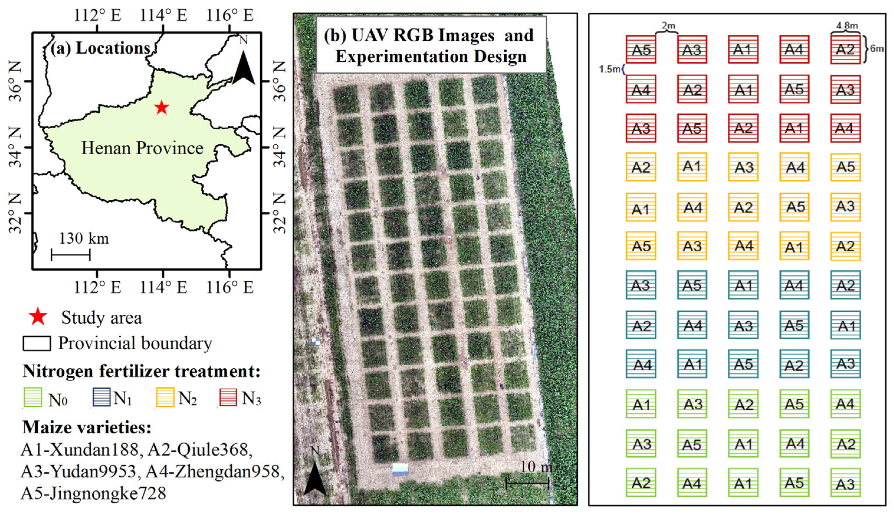
2.1. Study Area and Data

2.1.1. Study Area

The field experiment was conducted at the Smart Agriculture Demonstration Base of the Chinese Academy of Agricultural Sciences in Xinxiang County, Xinxiang City, Henan Province, China (35.2° N, 113.8° E; see Figure 1). The terrain in this region is predominantly flat, with a gentle rise from north to south. Geographically, the site forms part of the highly productive North China Plain, which is well known for intensive cereal cropping. The local climate is classified as a warm-temperate continental monsoon climate, with mean annual temperatures ranging from 14 °C to 27.3 °C and an average annual precipitation of approximately 573 mm. Notably, precipitation exhibits a strong seasonal pattern, with most rainfall occurring during the summer months.

The experiment was conducted during the 2024 summer maize growing season, which commenced with sowing in June and concluded with harvesting in October. Four nitrogen (N) fertilizer treatments were established along a north-to-south gradient, arranged in descending order of application rate: N₀: 0 kg N per mu, N₁: 5 kg N per mu, N₂: 10 kg N per mu, N₃: 15 kg N per mu. The experimental field was divided into 60 plots in a 12-row by 5-column arrangement, where every three rows constituted one N treatment zone. Each plot measured 4.8 m × 6.0 m, with buffer zones of 2.0 m between plots in the east–west direction and 1.5 m in the north–south direction to minimize edge effects. Five maize varieties were selected to represent a range of genetic backgrounds and agronomic characteristics (A1: Xundan188, A2: Qiule368, A3: Yudan9953, A4: Zhengdan958, and A5: Jingnongke728). Within each nitrogen treatment, each variety was replicated three times, ensuring robust statistical analyses of treatment effects. Figure 1 provides an illustrative overview of the experimental layout and plot arrangement.

2.1.2. UAV-Canopy Hyperspectral Data

A HeadWall MV.C VNIR hyperspectral imaging system (HeadWall Photonics, Bolton, MA, USA) served as the primary sensor for this study. The VNIR camera operates over a spectral range of 400–1000 nm, encompassing 342 distinct spectral channels, each at 1.75 nm sampling intervals and with a full-width-at-half-maximum (FWHM) of approximately 6 nm. Equipped with a CMOS detector, the camera provides a spatial resolution of 1024 pixels. Its fully reflective, concentric-aberration-corrected optical design (f/2.5) enhances imaging fidelity by minimizing optical distortions and maximizing signal throughput. Data transmission for the VNIR camera is supported via a USB 3.1 interface. The hyperspectral camera was mounted on a DJI Matrice 300 RTK (M300 RTK, Shenzhen, China), a quadcopter UAV system widely used for precision agricultural applications. The UAV’s dimensions are 810 mm × 670 mm × 430 mm (length × width × height), with a diagonal motor wheelbase of 895 mm. Its base weight, including dual batteries, is 6.3 kg, while the maximum takeoff weight can reach 9 kg. With a single-gimbal damping assembly capable of carrying up to 930 g, the platform readily accommodates the hyperspectral payload required for field-scale data acquisition.

Multi-temporal hyperspectral imagery was collected at two critical growth stages of maize during the 2024 growing season, namely the big trumpet stage (6 August) and the spinning stage (14 August). These particular phenological periods were chosen because they represent key developmental phases for maize, where physiological changes are most pronounced and therefore most informative for remote sensing–based assessments. To ensure data quality and inter-comparability, all flights were conducted under clear skies with wind speeds below 3 m/s, typically between 11:00 and 14:00 local time. This timing ensured optimal solar altitude angles, thereby minimizing shadow effects and maximizing reflectance signal consistency across the study plots. Such multi-temporal measurements are vital for capturing the dynamics of maize growth, facilitating advanced studies on crop stress, nutrient status, and yield estimation under different management regimes.

After capturing the initial hyperspectral UAV imagery, a structured series of preprocessing operations is essential to obtain reliable reflectance data for each maize plot. First, the high-accuracy onboard GPS/IMU data are combined with uniformly distributed ground control points (GCPs) to perform rigorous geometric and orthorectification corrections, ensuring centimeter-level positional precision. Following this, a comprehensive radiometric calibration and atmospheric correction is carried out to convert raw digital number (DN) values into surface reflectance. During this phase, reference panel measurements (recorded prior to takeoff) are used to correct for sensor-specific biases, thereby generating hyperspectral reflectance images that closely capture the actual spectral signatures of the canopy. Subsequently, ENVI software (Version 5.3.1) is employed to delineate each experimental plot as the fundamental unit of analysis. By aggregating all pixels within a plot boundary and computing their average reflectance value, representative canopy-level spectra are derived for each plot. The ratio of field training to validation set was 2:1, the number of training samples was 40, and the number of validation samples was 20 based on randomization.

2.1.3. Leaf Chlorophyll Content and Other Data

In this study, a spectrophotometric (chemical) method was employed to measure the chlorophyll levels in maize leaves, thereby providing both highly precise reference data and rapid field-based assessments. Chemical (Spectrophotometric) Method: Following standard procedures, two representative plants were selected from each experimental plot. From each plant, the third, seventh, and eleventh functional leaves (counted from the top) were sampled to capture potential vertical variations in chlorophyll content. To ensure sample consistency, 48 leaf discs (each 6 mm in diameter) were punched from the central portion of each leaf, avoiding the main vein, for a total leaf disc area of approximately 14 cm² per leaf position. These discs were immediately placed in 80 mL of 75% ethanol and kept under dark conditions for 5–6 days to facilitate complete chlorophyll extraction. Chlorophyll absorbance was measured using a 752 UV–Vis spectrophotometer (Hinotek, Ningbo, China). Prior to data collection, the instrument was warmed up for 30 min to achieve thermal equilibrium. The absorbance of each extract (in triplicate) was measured at 645 nm and 663 nm. The total chlorophyll content (C_ab) was computed using Equation (1), where the individual chlorophyll a (C_a) and chlorophyll b (C_b) concentrations were obtained via Equations (2) and (3) [42]:

$${\mathrm{C}}_{\mathrm{a}\mathrm{b}}={\mathrm{C}}_{\mathrm{a}}+{\mathrm{C}}_{\mathrm{b}}$$

(1)

$${\mathrm{C}}_{\mathrm{a}}=(12{.72\mathrm{A}}_{663}-2.59{\mathrm{A}}_{645})\times [\mathrm{V}/(1000\times \mathrm{W}\left)\right]$$

(2)

$${\mathrm{C}}_{\mathrm{b}}=(2{2.88\mathrm{A}}_{645}-4.67{\mathrm{A}}_{663})\times [\mathrm{V}/(1000\times \mathrm{W}\left)\right]$$

(3)

where ${\mathrm{A}}_{645}$, ${\mathrm{A}}_{663}$ are the absorbances at 645 nm and 663 nm, respectively, V is the volume of the extract (mL), and W is the total area (cm²) of the leaf discs.

2.2. Overview of Methods

Figure 2 illustrates a technical flowchart of this research, as detailed below:

• Dataset collection: UAV hyperspectral systems and spectrophotometers were used to obtain a total of 120 canopy spectral data (Section 2.1.2) and leaf chlorophyll data (Section 2.1.3) over two fertility stages. The PROSAIL model was used to simulate leaf spectral data (Section 2.3).
• Band selection: To identify bands that are sensitive to LCC and resistant to structural effects, the E2D-COS method (Section 2.4) was used and analyzed in combination with radiative transfer model simulation data (Section 2.3).
• Model pre-training: The simulated spectral data was employed to pre-train the DNN model to learn the potential knowledge of spectral versus vegetation traits, i.e., to get the model weights of the pre-trained model (Section 2.5.1 and Section 3.3.1).
• Model fine-tuning based on transfer learning: The weights of the pre-trained model are used as initial values for the model, which is again de-trained based on the field measured spectral data to fine-tune the part parameters of model (Section 2.5.2 and Section 3.3.2).
• Comparison of other methods: This study compared the performance of (1) the Mazie-LCNet trained on simulated and field measured data, (2) LCNet model trained on simulated dataset, (3) an Maize-LCNet-Field trained on field measured data, and (4) traditional statistical regression methods in estimating the maize LCC (Section 2.5.3 and Section 3.3.3).

2.3. Maize Canopy Spectral Simulation Using PROSAIL

The PROSAIL model, widely regarded as a foundational tool for simulating vegetation canopy spectra, couples the PROSPECT leaf optical properties model with the SAIL bidirectional reflectance canopy model [43,44]. In this study, we employed version 2.0.5 of the PROSAIL Python library (Version 2.0.5) to generate simulated canopy spectra of maize at multiple growth stages, aligning with the requirements bands selection (sensitive band screening (Section 2.4 and Section 3.1), structural interference spectral analysis (Section 2.4 and Section 3.2) and transfer learning (Section 2.5 and Section 3.3) of the research. The reason for choosing PROSAIL is that this model has been successfully used in many tasks of estimating physiological and biochemical parameters of crops, such as leaf area index [45], chlorophyl [46], and nitrogen [47]. At the same time, compared with some complex radiative transfer models (e.g., the LESS model [48]), the PROSAIL model is computationally efficient and has a low parameter requirement. Key model parameters—such as leaf area index (LAI), leaf angle distribution (LAD), and leaf chlorophyll content—were set according to field-based biophysical measurements and established references [24,32], ensuring that the simulations closely reproduced in situ spectral characteristics of maize canopies. Moreover, site-specific soil reflectance spectra, obtained directly from the experimental field, were incorporated to enhance both the realism and regional applicability of the results. Detailed model parameter values for big-bell-mouth stage and silking stage are given in

Table 1. Settings of the PROSAIL.

Parameters	Units	Big Trumpet Stage		Spinning Stage
		Transfer Learning	Bands Selection	Transfer Learning	Bands Selection
Leaf structure index (N)	unitless	1.2–1.6 (0.2)	1.5	1.2–1.8 (0.3)	1.7
Chlorophyll a + b content (Chl)	μg/cm2	20–90 (2)
Carotenoid content (Car)	μg/cm2	Cab/5
Equivalent water thickness (Cw)	cm	0.015–0.025 (0.002)	0.018	0.02–0.035 (0.002)	0.022
Dry matter content (Cm)	g/cm2	0.003–0.009 (0.001)	0.008	0.006–0.012 (0.002)	0.012
Leaf area index (LAI)	m2/m2	2–5 (0.5)	1.0–8.0 (1)	2.5–5 (0.5)	1.0–8.0 (1)
Average leaf inclination angle (LA)	Deg (°)	10–60 (10)	10–80 (10)	10–60 (10)	10–80 (10)
Solar zenith angle (SZA)	Deg (°)	45
Observer zenith angle (OZA)	Deg (°)	0

.

After parameterizing the model, a simulated dataset of 190,512 (Big trumpet stage) and 132,192 (Spinning stage) samples was generated. Each simulation included a high-resolution canopy reflectance spectrum and corresponding leaf biochemical parameters. A comprehensive quality-control procedure was carried out to remove any data points that did not conform to empirical observations. From each of the two growth stages, in order to increase the training efficiency of the model and reduce the computational performance requirements, 10,000 spectra were randomly selected to pre-train a neural network using transfer learning techniques. The ratio of training to validation set was 2:1, the number of training samples was 6666 and the number of validation samples was 3334 based on randomization. To facilitate two-dimensional correlation spectroscopy analyses, representative simulations were selected to investigate how leaf chlorophyll content (LCC) responds to variations in biophysical parameters under different canopy conditions. Specifically, (1) Screening of LCC sensitive bands using fixed-LAI and LA spectral data: big trumpet stage (LAI = 2.5, LA = 45°) and spinning period (LAI = 4, LA = 45°); (2) Band screening for resistance to structural interference using fixed-field measured spectral data of non-structural parameters (LAI and LA): for LAI, big trumpet stage (N = 1.5, C_w = 0.018, C_m = 0.008, LA = 45°, LAI = 1:8) and spinning period (N = 1.7, C_w = 0.08, C_m = 0.012, LA = 45°, LAI = 1:8). For LA, big trumpet stage (N = 1.5, C_w = 0.018, C_m = 0.008, LA = 10:60°, LAI = 2.5) and spinning period (N = 1.7, C_w = 0.08, C_m = 0.012, LA = 10:60°, LAI = 4). The resulting two-dimensional correlation spectra were analyzed to identify stable spectral regions that are minimally affected by changes in canopy structure. These stable regions can serve as robust spectral indices for LCC estimation, even when the canopy structure is subject to significant variation.

2.4. Enhanced Two-Dimensional Correlation Spectral Analysis (E2D-COS)

To select the sensitive spectral bands, E2D-COS is chosen for band screening in this paper. The reason for the selection is that it not only has the advantages of high efficiency and simple implementation, but also the method is highly sensitive to subtle spectral variations and can accurately quantify the interactions between bands for the purpose of separating sensitive bands [25,26]. The method has been successfully used in a variety of parameter estimation studies [24]. The specific steps are as follows: we first apply the spectral enhancement methods from Section 2.4.1 to preprocess the spectral data. Then, the 2D Correlation Spectroscopy Analysis plug-in is used to generate synchronous (Synchronous 2D-COS) and asynchronous (Asynchronous 2D-COS) spectra (Section 3.2.2). The resulting technique, termed enhanced two-dimensional correlation spectroscopy analysis (E2D-COS), combines these 2D correlation analyses with the improved spectral data.

2.4.1. Spectral Response Enhancement

Building on the classical two-dimensional correlation spectroscopy (2D-COS), Zhang et al. [24] proposed an amplitude- and shape-enhanced 2D-COS analysis approach (E2D-COS) to increase the sensitivity of hyperspectral data to external perturbations (e.g., changes in LCC, LAI, and LA). By jointly considering both the reflectance amplitude and the first derivative (i.e., the shape) of the hyperspectral curve, this method highlights subtle spectral features that may be overlooked if only a single facet of the spectrum is analyzed. The enhanced approach consists of four main steps:

✓

Spectral Normalization

To control for the constant incremental changes in the perturbation variable (LCC), raw hyperspectral reflectance values are normalized using the min–max method, as shown in Equation (4):

$$a_i={\displaystyle \frac{r_i-r_{min}}{{r_{max}-r}_{min}}}$$

(4)

where $r_i$ is the reflectance at the $i$-th band, and $r_{min}$ and $r_{max}$ are the minimum and maximum reflectance within that specific spectrum, respectively.

✓

First Derivative of the Spectrum

The first derivative of the normalized reflectance spectrum captures changes in slope and helps reduce the influence of background noise. Using the finite difference method, the first derivative ($\theta$) at $i$-th band is calculated as in Equation (5):

$$\theta ={\displaystyle \frac{a_{i+1}-a_i}{{\lambda }_{i+1}-{\lambda }_i}}$$

(5)

where $a_{i+1}$ and $a_i$ are the normalized reflectance at wavelengths ${\lambda }_{i+1}$ and ${\lambda }_i$, respectively.

✓

Response Relationship Computation

Pearson correlation coefficients are then calculated to quantify (I) the relationships between the normalized reflectance ($a_j$) and LCC, and (II) the first derivative (${\theta }_j$) and LCC, as shown in Equations (6) and (7):

$$r_a={\displaystyle \frac{{\Sigma }_{j=1}^n\left[\left(a_j-\overline{a}\right)\left(y_i-\overline{y}\right)\right]}{\sqrt{{\sum }_{j=1}^n{\left(a_j-\overline{a}\right)}^2}\sqrt{{\sum }_{j=1}^n\left(j-\overline{y}\right)}}}$$

(6)

$$r_{\theta }={\displaystyle \frac{{\Sigma }_{j=1}^n\left[\left({\theta }_j-\overline{\theta }\right)\left(y_i-\overline{y}\right)\right]}{\sqrt{{\sum }_{j=1}^n{\left({\theta }_j-\overline{\theta }\right)}^2}\sqrt{{\sum }_{j=1}^n{\left(y_i-\overline{y}\right)}^2}}}$$

(7)

where $r_a$ and $r_{\theta }$ represent the Pearson correlation coefficients of LCC with the normalized reflectance and its first derivative, respectively; $a_j$ and ${\theta }_j$ are the reflectance and derivative values for j-th sample, $a$ and $b$ are the respective mean reflectance and mean derivative over all samples; $y_i$ is the LCC value for sample; $y$ is the mean LCC of the sample set; and $n$ is the total number of samples.

✓

Enhanced Dynamic Spectrum Computation

Finally, the enhanced dynamic spectrum ($D$) is constructed by integrating the correlation coefficients ($r_a$) and first derivative ($r_{\theta }$) with the original reflectance ($r_i$), as given in Equation (8):

$$D=r_a+r_{\theta }+r_i$$

(8)

where $D$ is the enhanced dynamic spectrum, and $r_a$, $r_{\theta }$ and $r_i$ represent original reflectance, the Pearson correlation coefficients of LCC with the normalized reflectance and its first derivative. This additive integration of amplitude and shape information provides a more robust and sensitive spectral measure that highlights features most responsive to chlorophyll variation, effectively improving subsequent 2D correlation analyses. By emphasizing wavebands that exhibit high sensitivity to LCC, the enhanced approach helps elucidate key spectral drivers underlying chlorophyll dynamics and enhances the reliability of downstream applications such as vegetation health assessment and biochemical parameter retrieval.

2.4.2. Two-Dimensional Correlation Spectral Analysis

Conventional one-dimensional (1D) spectral analysis has certain limitations in handling complex spectral data. First, it struggles with overlapping spectral bands arising from multiple constituents, making it difficult to accurately identify and separate individual spectral features. Second, 1D methods often exhibit insufficient sensitivity to subtle variations in spectral data, potentially overlooking important spectral information. Moreover, they cannot intuitively reveal the interrelationships among different wavelengths, which constrains deeper investigation into the underlying mechanisms of spectral response.

Two-dimensional correlation spectroscopy (2D-COS) addresses these issues by introducing a second spectral dimension, thereby uncovering additional hidden information in the data. This method consists primarily of two core components: the synchronous spectrum and the asynchronous spectrum. The synchronous spectrum reflects the similarity of intensity changes across different wavelengths, whereas the asynchronous spectrum captures the sequential order of these changes. This technique offers several advantages: (1) by expanding 1D spectra into a two-dimensional map, it significantly enhances spectral resolution and helps isolate overlapping peaks; (2) it identifies dynamic features of spectral changes, highlighting minor structural variations within the sample; and (3) it reveals correlations among different wavelengths, providing critical insights into the mechanisms that drive the observed spectral responses.

By supplying multidimensional information about molecular vibrational modes, 2D-COS can extract weak peaks, shift peaks, and overlapping peaks. According to theory, the intensity of the dynamic spectrum is represented by $S$, $v$ as the variable and $t$ as the external perturbation, measured over $m$ steps with equal increments ($∆t$). The general expression is given in Equation (9):

$$S_{\left(v\right)}=\left(\begin{array}{c}{\displaystyle \genfrac{}{}{0pt}{}{y\left(v,t_1\right)}{y\left(v,t_2\right)}}\\ y\left(v,t_3\right)\\ .\\ .\\ .\\ y\left(v,t_m\right)\end{array}\right)$$

(9)

The synchronous and asynchronous 2D correlation intensities between two frequencies $v_1$ and $v_2$ are denoted by $\varphi \left(v_1,v_2\right)$ and $\phi \left(v_1,v_2\right)$, respectively, and can be computed using Equations (10) and (11):

$$\varphi \left(v_1,v_2\right)={\displaystyle \frac{1}{m-1}}{s}_{{\left(v_1\right)}^T\cdot s_{\left(v_2\right)}}$$

(10)

$$\phi \left(v_1,v_2\right)={\displaystyle \frac{1}{m-1}}{s}_{{\left(v_1\right)}^T\cdot D\cdot s_{\left(v_2\right)}}$$

(11)

where $w_{\left(v_1,v_2\right)}$ is the combined 2D correlation intensity obtained by multiplying the synchronous and asynchronous correlation intensities:

$$w_{\left(v_1,v_2\right)}=\left[\varphi \left(v_1,v_2\right)\right]\cdot \left[\phi \left(v_1,v_2\right)\right]$$

(12)

In these expressions, $D_{jk}$ is the Hilbert–Noda transformation matrix; for row j and column k, its elements are defined as follows (Equation (13)):

$$D_{jk}=\left\{\begin{array}{cc}\hfill 0,& j=k\hfill \\ {\displaystyle \frac{1}{\pi \left(k-j\right)}},& j\ne k\hfill \end{array}\right.$$

(13)

Additionally, the dataset used in this study derives from both in situ measurements and PROSAIL-simulated data. The simulated dataset is leveraged to compensate for the limited LCC gradient in the measured data, ultimately improving the effectiveness of E2D-COS. Specifically, the PROSAIL dataset ranges from 20 to 90 µg/cm² in 2 µg/cm² increments of chlorophyll content, covering the majority of observed spectral scenarios. This study primarily utilizes the synchronous spectrum to identify characteristic wavelengths linked to maize canopy LCC. Through highlighting dynamically responsive spectral features, E2D-CSA deepens our understanding of canopy reflectance mechanisms and provides a basis for a more accurate retrieval of key biochemical parameters.

2.5. Modeling Methods

2.5.1. Deep Neural Network

A deep neural network (DNN) can be viewed as a multilayer feedforward neural architecture designed to capture high-level feature interactions from input data through successive layers of processing. When each layer in a DNN is fully connected, every neuron in one layer links to every neuron in the subsequent layer. By systematically increasing the number of hidden layers, the model gains the capacity to discern and learn more complex patterns, which can improve predictive performance for regression or classification tasks under certain conditions [49]. The reason for choosing DNN is that compared to currently commonly used models such as RF, and more complex DL models, DNN models adaptively extract spectral features through hierarchical non-linear transformations, overcoming the limitations of traditional methods that rely on manual feature engineering [50], while avoiding the modelling of invalid spatial correlations by complex DL networks [51].

In this work, we employed a five-layer DNN (Figure 3) to estimate the leaf nitrogen content (LNC). The structure comprises a single input layer, three hidden layers, and an output layer. All layers are fully connected; specifically, the final output layer regresses the LNC based on the feature representations obtained in the hidden layers. Since this design does not inherently utilize spatial information, the input layer accepts only one-dimensional vectors, where each sample’s features (e.g., reflectance bands and other ancillary attributes) have been concatenated into a single vector. To harmonize feature magnitudes, we apply Z-score normalization, which recalibrates each feature $x$ to $(x-\mu )/\sigma$, where $\mu$ is the mean and $\mu$ is the standard deviation. Model learning proceeds by forward propagation of inputs through each hidden layer, with intermediate activations producing non-linear transformations of the data. Ultimately, the last layer generates a linear output that corresponds to the predicted LNC. The training objective employs the root mean squared error (RMSE) as the loss function, augmented with an L2 regularization term to reduce overfitting:

$$L={\displaystyle \frac{1}{n}}{\sum }_{i=1}^n{\left(y_{true}^i-y_{esti}^i\right)}^2+{\displaystyle \frac{c}{2n}}{‖w‖}_2^2$$

(14)

$${‖w‖}_2^2={\sum }_{j=1}^n{w}_j^2=w^{T}w$$

(15)

where $n$ is the number of training samples, $y_{true}^i$ and $y_{esti}^i$ denote the observed and predicted LNC values for sample iii, respectively, $c$ is a penalty coefficient, and $w$ is the vector of model weights. By backpropagating the error calculated from this loss function, the model iteratively updates its parameters.

Overfitting can arise when the model complexity is high or when the training data are insufficient. To counteract this risk, we incorporate L2 regularization alongside a dropout mechanism, both of which can limit the model’s tendency to memorize training examples and enhance its ability to generalize. We also conduct grid-based tuning of the most influential hyperparameters, ensuring that the final DNN configuration strikes a balance between model capacity and robustness. The resulting architecture has proven effective for learning sophisticated feature representations from diverse spectral and auxiliary inputs, enabling precise regression of LCC values.

2.5.2. Transfer Learning

Transfer learning (TL) generally describes a process wherein expertise acquired through solving one task is leveraged to enhance performance on another related task. This strategy is particularly useful for mitigating the limitations associated with applying a model trained in one setting directly to new or varying environments, a problem often termed the “domain shift.” By integrating TL, researchers can minimize the reliance on extensive labeled datasets from each new context, thereby addressing discrepancies in data characteristics across different neighborhoods or study sites [52]. Over the past few years, TL has become increasingly prevalent in the remote sensing domain, proving instrumental for applications such as land cover classification [53], monitoring vegetation dynamics [36] estimating soil properties [54], and predicting disease variations [55]. In this work, we initially trained the DNN on simulated datasets generated by PROSAIL to enable the model to learn LCC estimation capabilities (LCNet). During the subsequent model adaptation, the weights of the first two hidden layers (HL1 and HL2) acquired in the pre-training phase served as fixed parameter values; and the last hidden layer (HL3) weights served as initial parameter values; these were then optimized using the field-measured spectra (Section 2.1.2), thus refining the model for practical, real-world application (Maize-LCNet).

2.5.3. Comparison of Methods

In addition to the proposed method for estimating the canopy LCC of maize, we tested the performance of the pre-trained model using simulated data (LC-Net), and PLSR/RF methods for quantitative validation.

• LCNet: Pre-trained models trained on simulated data (n = 6666) directly estimate the field validation dataset (n = 20) to evaluate their performance.
• Maize-LCNet-field methods: DNN trained on field data (n = 40) directly estimate the field validation dataset (n = 20) to evaluate their performance.
• PLSR/SVM-field methods: Based on the spectral data measured in the field (n = 40), linear and non-linear machine learning algorithms (PLSR and SVM) are used to train the model and verify its accuracy.

2.6. Assessing Accuracy

To assess the predictive quality of our model in estimating LCC, we adopted two commonly used performance metrics: the coefficient of determination (R²), and the root means square error (RMSE). In essence, R² quantifies how closely the predictions align with real observations—higher values indicate a stronger match. RMSE reflects the average magnitude of errors between predicted and observed values, providing an overall sense of accuracy.

3. Results

3.1. Sensitive Bands of LCC

3.1.1. Characteristics of the Simulated Spectral Data

Figure 4 presents simulated canopy reflectance curves for the big trumpet stage and the spinning stage. These simulated spectra encompass nearly the full breadth of the in situ reflectance measurements acquired at each developmental phase. A pronounced “green peak” emerges around 550 nm, attributable to intense chlorophyll and carotenoid absorption in the blue and red bands contrasted with relatively weaker absorption in the green region. Around 690 nm, there is a marked rise in reflectance (the “red edge”), a known indicator of photosynthetic pigment content transitioning into the near-infrared reflectance plateau. An evident dip near 960 nm is further observed and is generally associated with water vapor absorption, reflecting both atmospheric effects and canopy moisture content.

Figure 5 illustrates the reflectance distribution at five representative wavelengths—450 nm (blue), 550 nm (green), 650 nm (red), 740 nm (red edge), and 800 nm (near-infrared)—across each growth stage. These results confirm that the spectral variability in the simulated dataset extends to practically all reflectance values measured in the field. By spanning these critical wavebands, the simulations demonstrate broad coverage and strong representativeness of actual canopy reflectance dynamics throughout the crop growth cycle. Collectively, these findings underscore the suitability of the simulated dataset for investigating the spectral behavior of maize canopies and for supporting advanced modeling of plant physiological traits.

3.1.2. Enhanced Two-Dimensional Correlation Spectral Analysis of Canopy LCCs

Figure 6 presents the synchronous spectra derived from the E2D-COS methodology, shedding light on how canopy reflectance in maize responds to variations in leaf chlorophyll content (LCC) at distinct developmental phases. In the big trumpet stage, the number of self-correlation peaks increases to 11, detected at 418 nm, 453 nm, 506 nm, 566 nm, 587 nm, 640 nm, 688 nm, 767 nm, 802 nm, 829 nm, and 956 nm. Compared with the jointing stage, additional key wavelengths arise in the visible region (416–688 nm), especially in the green band (506–587 nm), suggesting that changes in LCC exert a heightened influence on reflectance in this spectral window. Likewise, the near-infrared range (767–956 nm) shows intensified correlations, reflecting more intricate canopy-level interactions as the crop transitions toward more developed structural forms. By the spinning stage, the synchronous spectrum features 11 self-correlation peaks at 418 nm, 453 nm, 541 nm, 559 nm, 688 nm, 723 nm, 767 nm, 832 nm, 878 nm, 956 nm, and 994 nm. Notably, the near-infrared interval (767–994 nm) encompasses a broader set of sensitive wavelengths, with correlation intensities reaching their highest levels. Such strong near-infrared responses likely stem from the canopy’s relatively stable structure during reproductive growth, wherein variations in LCC manifest more markedly through overall reflectance changes. Additionally, the enduring sensitivity in the 688–723 nm red-edge domain highlights its ongoing prominence in tracking LCC fluctuations.

In summary, these two stages collectively illustrate a trend in which reflectance characteristics initially concentrate around the red and red-edge bands, then expand to broader spectral regions as maize development progresses. The growing importance of near-infrared features underscores the complex interplay between biochemical and structural factors in the canopy. These findings not only validate the utility of E2D-COS for delineating stage-specific responses to LCC but also offer actionable insights for selecting spectral features of the estimation model aimed at improved chlorophyll estimation in maize.

Figure 7 illustrates the asynchronous enhanced two-dimensional correlation spectroscopy (E2D-COS) outcomes, thereby revealing the sequential relationships underlying canopy reflectance variations across different maize growth stages. Comparative analysis of the three asynchronous E2D-COS maps demonstrates a clear evolution in spectral response characteristics as the crop develops. In the big trumpet stage, this alternating “red–blue” pattern becomes concentrated within a narrower 705–744 nm window, with higher correlation intensities pointing to more pronounced sequential differences among wavebands in that interval. By the spinning stage, asynchronous correlation intensities reach their highest levels (±0.05), especially between 703 nm and 735 nm, where the red–blue oscillations are most pronounced.

This systematic progression of asynchronous correlations aligns strongly with the synchronous E2D-COS findings, reinforcing the importance of these wavebands in tracking chlorophyll dynamics. Moreover, the observed shift in the timing of spectral responses—gradually converging around the red-edge region as the plant advances through its phenological stages—highlights the crucial role of red-edge reflectance in chlorophyll estimation. These insights not only corroborate the selection of key diagnostic wavelengths but also illuminate the temporal sequencing of spectral changes, offering critical theoretical underpinnings for refining stage-specific chlorophyll inversion models in maize.

3.2. Screening Results for Structural Interference Signature Bands

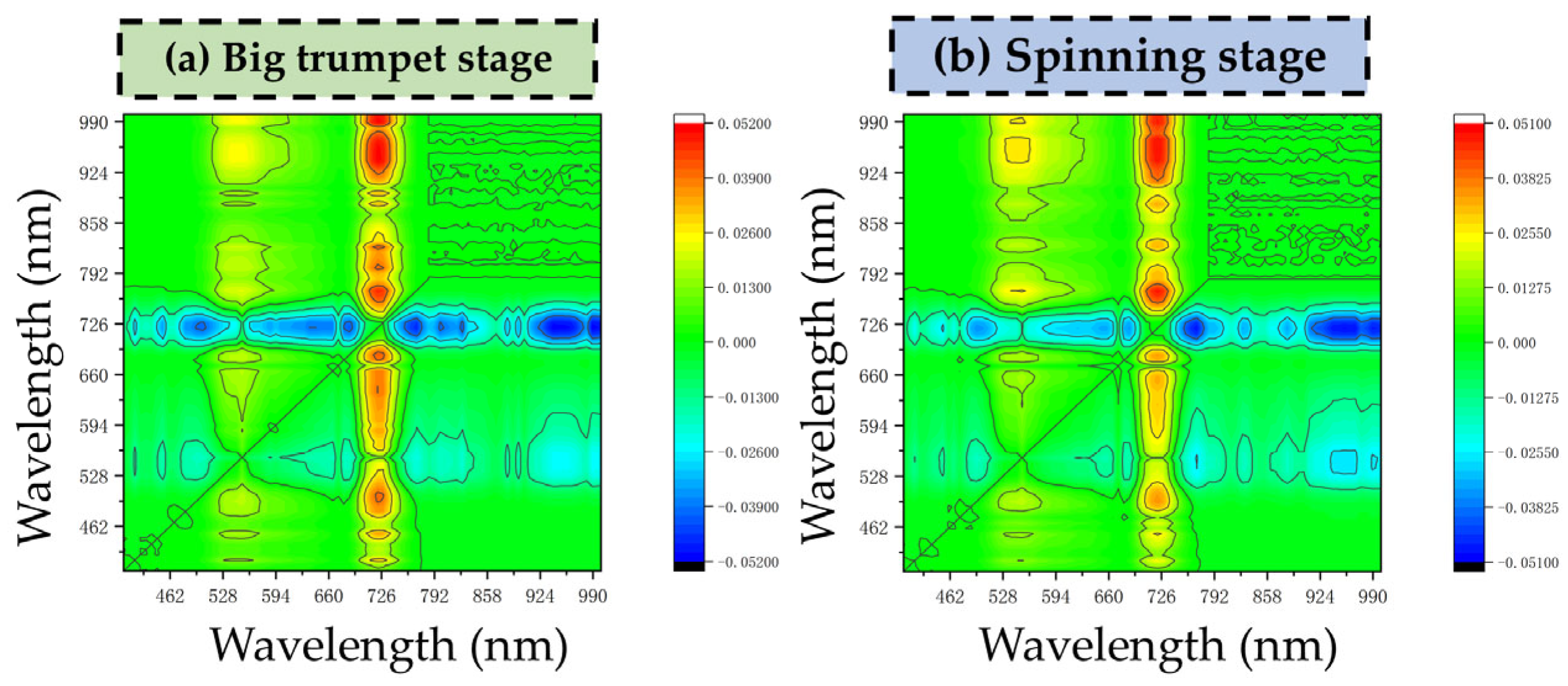
3.2.1. Enhanced Two-Dimensional Correlation Spectral Analysis of LAI

In the remote sensing inversion of vegetation physiological parameters, it is crucial that waveband selection be primarily driven by the target variable rather than confounding influences. In particular, leaf chlorophyll content (LCC) and leaf area index (LAI) each govern distinct processes in photosynthesis—LCC predominantly dictates the absorption of solar radiation, whereas LAI modulates how effectively a canopy intercepts incoming light. Together, these two parameters exhibit considerable coupling effects on canopy reflectance. Consequently, identifying wavebands highly sensitive to LCC while only marginally impacted by LAI is essential for enhancing the accuracy of retrieval models.

This study employed the PROSAIL model to simulate canopy reflectance at two critical phenological stages of maize—the big trumpet stage and the spinning stage. Over an LAI range of 1–8, LCC was systematically varied from 20 to 90 μg/cm² in increments of 2 μg/cm², thereby illuminating how the spectral signatures shift in response to LCC. We then applied an enhanced two-dimensional correlation spectroscopy (E2D-COS) approach to probe the spectral response patterns under different LAI levels. Figure 8 and Figure 9 present the synchronous E2D-COS maps generated at each growing stage, providing insights into the consistent spectral features that are most indicative of LCC changes across diverse canopy structures. These findings form a robust basis for refining inversion strategies aimed at accurately estimating LCC, even when LAI varies substantially.

✓

The synchronous E2D-COS maps of the big trumpet stage with various LAIs

Figure 8i summarizes the evolution of self-correlation peak positions under different LAI conditions of the big trumpet stage. At this stage, the number of self-correlation peaks in the visible range increases substantially, producing a dense cluster of stable wavebands (418 nm, 453 nm, 506 nm, 566 nm, and 587 nm) that remain largely unaffected by changes in LAI. Compared with the jointing stage, red-edge peaks (640–688 nm) also show greater positional stability, implying that canopy structure exerts diminished influence on red-edge reflectance at this point in development. The near-infrared region evolves from multiple discrete self-correlation peaks (767–985 nm) at lower LAI values (e.g., LAI = 1 or LAI = 2) to a more concentrated set of stable peaks (767 nm, 802 nm, 829 nm, and 954 nm) at higher LAI values. Thus, LAI changes during this period mainly affect wavelengths beyond 767 nm. Consequently, the big-bell-mouth stage wavebands that demonstrate minimal LAI sensitivity include 418 nm, 453 nm, 506 nm, 587 nm, 640 nm, 688 nm, and 767 nm.

✓

The synchronous E2D-COS maps of the spinning stage with various LAIs

By the silking stage, self-correlation peaks become fewer but more robust. Although the number of peaks in the visible region (418–559 nm) declines compared to earlier stages, their stability is markedly enhanced. The red-edge domain (688–723 nm) remains nearly stationary, reflecting a relatively mature and stable canopy structure. In the near-infrared range, scattered peaks at lower LAI values (767–985 nm) coalesce into a fixed set of characteristic peaks (e.g., 767 nm, 832 nm, 878 nm, 961 nm, and 996 nm) at higher LAI levels. This pattern echoes that observed at the big-bell-mouth stage, where LAI primarily influences wavelengths above 767 nm. Consequently, the silking-stage wavebands with minimal susceptibility to LAI include 418 nm, 453 nm, 541 nm, 559 nm, 688 nm, 723 nm, and 767 nm. Figure 9i depicts the specific peak positions under varying LAI conditions.

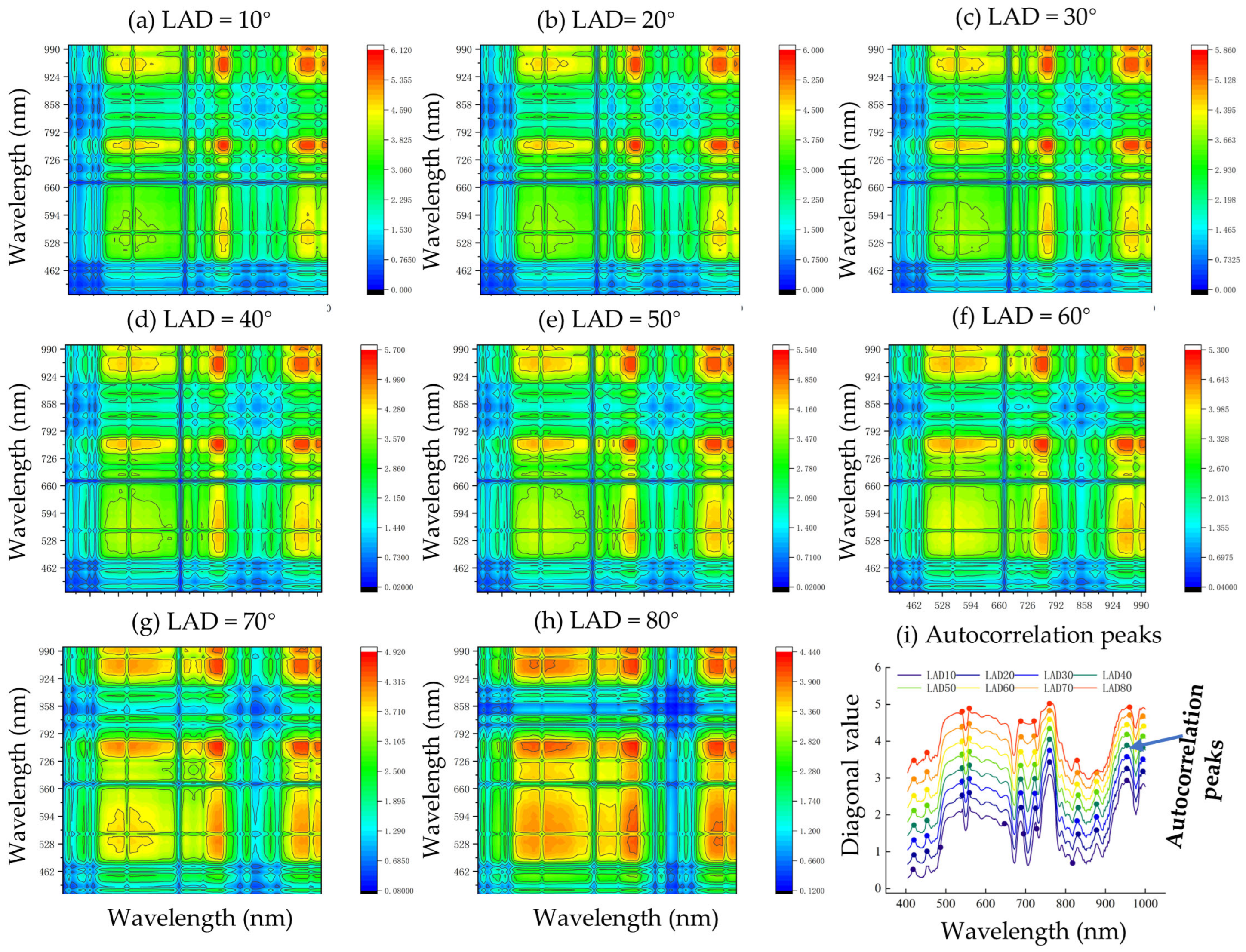
3.2.2. Enhanced Two-Dimensional Correlation Spectral Analysis of LA

Beyond leaf area index (LAI), variations in leaf inclination also shape the overall structure of a maize canopy. To clarify the impact of leaf angle distribution (LAD) on spectral signals, we simulated canopy reflectance using the PROSAIL model with an average leaf angle (ALA) range of 10–80°; leaf chlorophyll content (LCC) was systematically varied from 20 to 90 μg/cm² in increments of 2 μg/cm². Leveraging enhanced two-dimensional correlation spectroscopy (E2D-COS), we then analyzed the spectral response patterns under these diverse LAD configurations. Figure 10 and Figure 11 depict the synchronous E2D-COS plots for key phenological stages.

✓

The synchronous E2D-COS maps of the big trumpet stage with various LADs

The big trumpet stage demonstrates notably consistent spectral features (Figure 10). When the leaf angle (LAD) varies between 10° and 60°, the visible-range peaks (418 nm, 453 nm, 506 nm, 566 nm, and 587 nm) and red-edge peaks (640 nm and 688 nm) remain stable. The near-infrared region also exhibits relatively fixed peak positions at 767 nm, 802 nm, 829 nm, 954 nm, and 998 nm. However, for LAD values above 70°, additional NIR peaks (807 nm, 825 nm, 846 nm, 871 nm, 894 nm, 910 nm, and 985 nm) emerge. Consequently, wavebands at 418 nm, 453 nm, 506 nm, 566 nm, 587 nm, 640 nm, 688 nm, and 767 nm remain largely unaffected by moderate variations in leaf angle. Figure 10i illustrates the positions of these peaks under different LAD conditions.

✓

The synchronous E2D-COS maps of the spinning stage with various LADs

By the spinning stage, self-correlation peaks exhibit greater consolidation and enhanced stability (Figure 11). In the visible spectrum, wavebands around 418 nm, 453 nm, 541 nm, and 559 nm remain robust throughout the examined LAD range. The red-to-red-edge interval (approximately 688–760 nm) similarly shows consistent behavior, with only minor shifts (723–725 nm) at its lower boundary. In the near-infrared region, peaks near 828 nm change very little as LAD increases. Meanwhile, certain longer-wavelength peaks (for example, at 956 nm and 994 nm) do shift slightly at LAD values between 10° and 70°. Overall, wavebands at 418 nm, 453 nm, 541 nm, 559 nm, 688 nm, 723 nm, 767 nm, and 832 nm demonstrate minimal sensitivity to variations in canopy structure. Figure 11i illustrates these patterns within the range of leaf angles considered.

Summarize Section 3.2: The E2D-COS analysis identifies wavebands that strongly correlate with LCC yet exhibit limited sensitivity to LAD alterations. Specifically, during the big-bell-mouth stage, the optimal set comprises 418 nm, 453 nm, 506 nm, 587 nm, 640 nm, 688 nm, and 767 nm. Finally, for spinning, wavebands at 418 nm, 453 nm, 541 nm, 559 nm, 688 nm, 723 nm, and 767 nm display robust resistance to canopy structural changes. These stable waveband combinations provide valuable guidance for improving remote-sensing models aimed at retrieving chlorophyll levels, with reduced interference from varying leaf angles and complex canopy architectures.

3.3. LCC Estimation Result

3.3.1. Pre-Training Based on Simulated Hyperspectral Reflectance Dataset

Table 2. The accuracy of simulated dataset of proposed LCNet of different stages in pre-training process of transfer learning.

Model	Stage	Train (n = 6667)		Validation (n = 3334)
		R2	RMSE (g/cm2)	R2	RMSE (g/cm2)
Pre-trained LCNet	Big trumpet stage	0.94	4.33	0.94	4.31
	Spinning stage	0.97	3.07	0.97	3.04

lists the train and validation accuracy results of the LC-Net of different stages utilizing simulated spectral data. The findings indicate that all pre-trained LC-Net models successfully achieved an accurate estimation of maize LCC (R²s above 0.94, RMSEs below 5 g/cm²). Figure 12 illustrates the pre-training estimated outcomes of the LC-Net network for different stages utilizing simulated spectral data. Figure 12a,d presents the variation in loss across epochs of the big trumpet stage and the spinning stage. The findings suggest that loss decreases rapidly during the first 5 epochs of training; during the subsequent training sessions (5–95 epochs), the change in loss becomes slow. This indicates that the model received significant convergence in the training process. The estimates and simulated inputs of train and validation in Figure 12b,c,e,f have strong consistency (slopes > 0.90, RMSEs < 5 g/cm²), which also indicates that the LC-Net model achieves an accurate estimation of maize LCC.

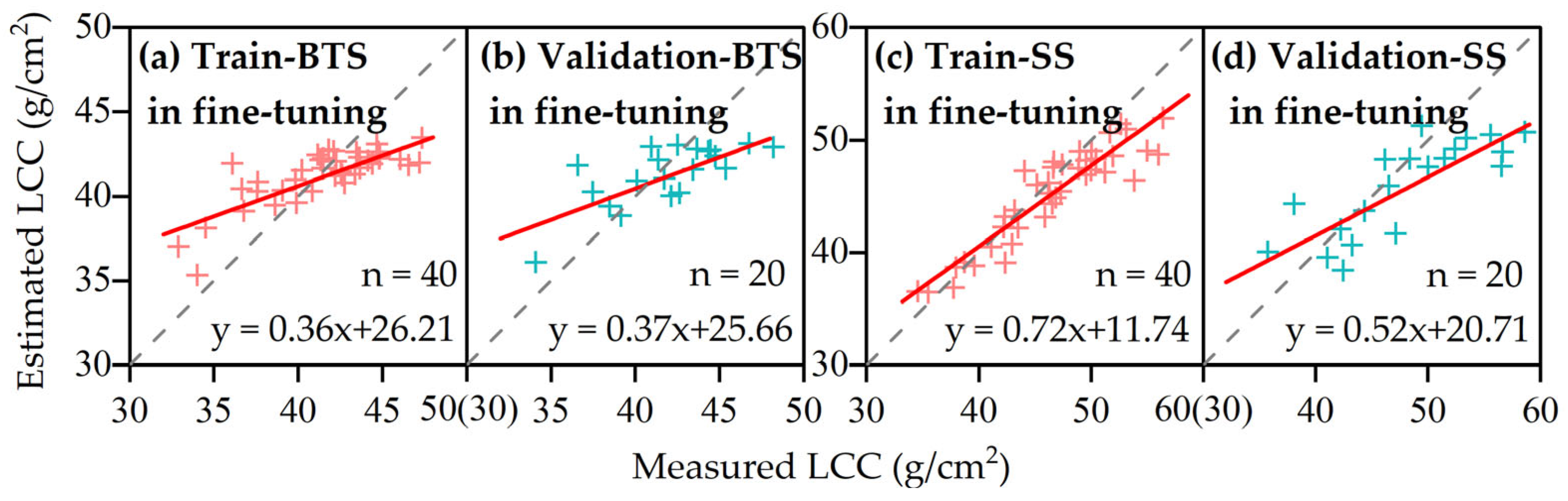
3.3.2. LCC Estimation Based on Transfer Learning

Applying transfer learning, the LC-Net network obtained from pre-training is again trained with the maize field spectral data to achieve the fine-tuning of the model (Maize-LCNet).

Table 3. The accuracy of field dataset of proposed Maize-LCNet with different stages in fine-tuning process of transfer learning.

Model	Stage	Train (n = 40)		Validation (n = 20)
		R2	RMSE (g/cm2)	R2	RMSE (g/cm2)
Maize-LCNet	Big trumpet stage	0.63	2.49	0.54	2.53
	Spinning stage	0.84	2.67	0.65	4.39

shows the train and validation accuracy of the fine-tuned Maize-LCNet. The performance of the estimation model was superior for both growth stages; the explanatory power and goodness-of-fit of the model for LCC were higher than 54% (54% to 84%), and the RMSE was below 5 g/cm². Figure 13 illustrates the fitting relationship between the estimated and measured values for each model. The differences in the degree of deviation from the 1:1 line and the accuracy metrics of the curve fits of the different model estimates to the measured data are consistent. Specifically, the R² of the SS was greater than 0.60, the fitted curve was closer to the 1:1 line, and the fitted slope was higher than 0.50, while the R² of the BTS was lower than 0.60, the fitted slope was lower than 0.40, and the RMSEs that could individually represent the errors of the different periods were all very low. Overall, the estimation ability of the SS model was superior to the BTS model; the training and validation accuracies R² of the SS stage model were 0.21 and 0.01 higher compared to the BTS model.

3.3.3. Estimation Results from Comparative Experiments

To demonstrate the effectiveness of the proposed model, comparison experiments were conducted and the validation accuracies of the pre-trained model (LC-Net) and the model trained using field data (PLSR-field/SVM-field) are shown in

Table 4. Validation results of multiple comparison methods.

Growth Stage	Accuracy Indicators		LCNet	Maize-LCNet-Field	PLSR-Field	SVM-Field
Big trumpet stage	Validation	R2	0.09	0.48	0.51	0.45
		RMSE (g/cm2)	3.61	3.59	2.52	2.55
Spinning stage	Validation	R2	0.17	0.54	0.62	0.55
		RMSE (g/cm2)	65.84	4.96	3.87	4.23

and Figure 14. The results showed that the pre-trained models (LC-Net) for both fertility stages performed poorly, with validation R² lower than 0.20 and RMSE higher than 3 g/cm², including very large RMSE errors (65.84 g/cm²) during the spinning stage (SS); the validation accuracies of the remaining three models (LC-Net-field, PLSR-field, and SVM-field) trained based on real data were all acceptable. The R² during the big trumpet stage (BTS) was greater than 0.45, and the RMSEs were all less than 4 g/cm², and the R² during the SS was all greater than 0.54, and the RMSEs were all less than 5. In contrast, the PLSR model had a higher accuracy, and both the LC-Net model and the SVM model performed poorly. The results of the estimated and measured values in Figure 14 also proved that the fitted line of the PLSR model was the closest to the 1:1 line; the fitted slopes were 0.65 to 0.72. The next best fit was Maize-LCNet-field, with fitted slopes of 0.65 to 0.68; and the other models apparently suffered from overall underestimation (Figure 14b,e,f), or local underestimation/overestimation (Figure 14a,d); the slopes of the fits were all below 0.50.

To clarify whether the estimation results of different models are statistically significant, paired t-tests between the proposed Maize-LCNet model and multiple comparative models were performed, and the results are given in

Table 5. Results of paired sample t-test between proposed Maize-LCNet and comparative model.

Comparison	Big Trumpet Stage		Spinning Stage
	t	p-Value	t	p-Value
Maize-LCNet vs. LCNet	0.468	0.645	2.421	0.026
Maize-LCNet vs. Maize-LCNet-field	4.289	0.000	49.619	0.000
Maize-LCNet vs. PLSR-field	−3.772	0.045	2.256	0.036
Maize-LCNet vs. SVM-field	−4.330	0.000	−0.285	0.779

. The results indicated that, except for the LCNet model of the BTS and the SVM-field model of the SS, the estimation results of Maize-LCNet were significantly different from the other models, with the degree of significance reaching 5% (p-value: 0.000 to 0.045), and the above results proved the validity of the proposed model.

4. Discussion

4.1. Advantages of the Estimation Method

Accurate real-time chlorophyll monitoring in maize canopies is critical for precision agriculture, enhancing fertilizer efficiency and yield stability. This study introduces an innovative deep learning architecture (Maize-LCNet) that synergistically integrates physical models, deep learning, and transfer learning for enhanced chlorophyll content quantification in maize canopies. Compared with existing studies, this study not only clarifies the spectral bands that are relevant to maize chlorophyll and resistant to structural influences, but also proposes an estimation method for high-performance estimation of maize chlorophyll content, with detailed findings as follows: (1) Effective spectral band selection: The integration of physical modeling with the E2D-COS method successfully identified chlorophyll-sensitive spectral bands. These bands enabled the development of a robust PLSR-based estimation model (R² = 0.62 at the spinning stage), demonstrating the feasibility of using E2D-COS and simplified regression approaches for canopy chlorophyll quantification, which is consistent with existing findings (R² = 0.61 in heading stage of wheat) [24]. (2) Simulation-to-reality transfer: The proposed Maize-LCNet model, fine-tuned with field data, significantly outperformed the simulation-only trained baseline (CC-Net), with R² increasing from 0.09–0.17 to 0.54–0.65 and RMSE decreasing from 3.61–65.84 to 2.53–4.39 g/cm². This highlights the necessity of domain adaptation to bridge the spectral gap between synthetic and real-world data. (3) Transfer learning efficacy: Compared to field-data-trained models (LCNet-field), Maize-LCNet achieved superior accuracy with R² improvements of 0.06–0.11 and RMSE reductions of 0.57–1.06 g/cm², validating the synergistic effect of combining pre-training on simulated data with targeted fine-tuning. The above results inform future estimation studies. Transfer learning is one way to improve model performance, consistent with the advocacy of existing research [52,56]. Meanwhile, the estimation results of the proposed Maize-LCNet model have lower errors (RMSE: 2.53 in the BTS) compared to the existing methods (RMSE: 4.14~4.46) [57]. (4) Comparative method performance: Traditional methods (PLSR, SVM) exhibited comparable accuracy to deep learning models (DNN), likely due to the optimized spectral features selected through physical guidance. This suggests that feature engineering remains crucial even in deep learning frameworks. These findings collectively demonstrate that Maize-LCNet, which integrated E2D-COS, RTM, field spectroscopy, and TL, provides a reliable solution for leaf chlorophyll content (LCC) estimation in maize. The model’s strong performance (R² = 0.65 in critical growth stages) underscores its potential for precision nitrogen management. Notably, our results align with recent studies [36,52] emphasizing that pre-training on large synthetic datasets followed by transfer learning significantly enhances model generalizability, particularly under limited field sampling conditions.

4.2. Optimized Bands for Maize Chlorophyll Estimation

The identification and optimization of sensitive spectral features play a pivotal role in ensuring robust performance for both regression and classification tasks in agricultural remote sensing. Traditional approaches, including vegetation indices [58], fractional derivative transformations [59], and recursive feature elimination [18], primarily rely on empirical spectral feature engineering derived from field measurements. While effective, these methods often face limitations in generalizability due to their dependency on site-specific data patterns. To address this challenge, our study introduces a physics-informed spectral optimization framework that synergizes enhanced E2D-COS with radiative transfer modeling, which not only ensures that the selected bands are resistant to structural influences, but at the same time responds significantly to canopy chlorophyll changes. The screened bands showed changes corresponding to the growth and development of maize: Big trumpet stage: dominated by the transition zone of the blue-green bands (418 nm, 453 nm, 506 nm), the valley of chlorophyll absorption (587 nm, 640 nm) and the early red edge (688 nm), reflecting the rapid growth of the leaves and the high demand for plant nutrients. Spinning stage: enhanced red-edge dynamics and near-infrared plateaus (688 nm, 723 nm, 767 nm), capturing canopy closure effects and photosynthetic optimization during reproductive phases. These findings of locations of chlorophyll-sensitive but resistant-to-structural-effects bands described above have similarities with existing studies (458 nm, 586 nm, 686 nm,690 nm, etc.) [60,61], but the present study uses radiative transfer modelling to clarify the rationale for the choice of this band. These bands collectively capture the spectral interplay between biochemical absorption and canopy structural development. The identification of these bands provides a reference for maize chlorophyll estimation studies.

4.3. Limitations and Future Directions

While this study demonstrates the feasibility of incorporating physical knowledge into deep neural networks (DNNs) for chlorophyll estimation, several limitations warrant attention. First, the DNN architecture may not fully capture the full complexity of radiative transfer processes, particularly the implicit parameter interactions within PROSAIL simulations. Future work should explore advanced architectures, such as convolutional neural networks (CNNs) or hybrid neural operators, to better model the hierarchical spectral–structural relationships inherent in canopy radiative transfer. Of course, although DNN model outperform the PLSR and SVM approach (Section 3.3.3), the use of DNN also increases the time and computational resources for model training, mainly because the DNN model structure is relatively complex compared to methods such as random forests, or simpler deep learning methods, and it is important to balance model complexity and cost in future research. Second, although the UAV-based hyperspectral platform meets farm-level precision agriculture requirements, its scalability to regional monitoring remains constrained. Satellite multispectral imagery—despite coarser spectral resolution—offers broader applicability. However, adapting our model to satellite data requires addressing cross-sensor generalization capabilities and atmospheric correction challenges.

5. Conclusions

The capacity to accurately monitor the health and growth of maize is of paramount importance for farmers and policymakers, as it plays a crucial role in guiding agricultural production and policy implementation. This study proposes a novel method for estimating maize leaf chlorophyll content (LCC) by integrating E2D-COS feature selection, transfer learning (simulated and field hyperspectral data), and the deep learning network (LCNet). The principal conclusions are summarized as follows: (1) The E2D-COS feature selection method combined with simulated data effectively identified structural interference-resistant spectral bands strongly correlated with maize LCC: Big trumpet stage: 418 nm, 453 nm, 506 nm, 587 nm, 640 nm, 688 nm, and 767 nm; Spinning stage: 418 nm, 453 nm, 541 nm, 559 nm, 688 nm, 723 nm, and 767 nm. (2) The E2D-COS-derived spectral bands enabled reliable LCC estimation across models, confirming the robustness of the feature selection methodology: The PLSR-based model achieved R² = 0.62 and RMSE = 3.87 g/cm and the CC-Net-field model yielded R² = 0.54 with RMSE = 4.96 g/cm. (3) The integration of E2D-COS feature selection with transfer learning and deep learning techniques significantly improved estimation accuracy: Compared to the CC-Net-field, the proposed Maize-LCNet model exhibited R² improvements of 0.06–0.11 and RMSE reductions of 0.57–1.06 g/cm. Compared to the existing studies, this study not only clarifies the spectral bands that are relevant to maize chlorophyll and resistant to structural influences, but also proposes an estimation method for high-performance estimation of maize chlorophyll content. The accurate estimation of chlorophyll content provides actionable insights for both farmers and policymakers. By monitoring real-time chlorophyll levels, farmers gain critical visibility into crop vitality, enabling data-driven better decisions on fertilization, irrigation, and pest management to optimize yield and resource efficiency. For governments, this information enables targeted policies to support precision agriculture and sustainable agricultural development. Certainly, the above method has limitations: the DNN may not fully capture spectral variations under chlorophyll changes, requiring more advanced architectures; UAV-based data also limits scalability, highlighting the need to address chlorophyll estimation at satellite scale in future work.

References

1. Tanaka, A.; Ito, H. Chlorophyll degradation and its physiological function. Plant Cell Physiol. 2024, 66, 139–152. [Google Scholar] [CrossRef]
2. Gao, F.; Guo, J.; Shen, Y. Advances from chlorophyll biosynthesis to photosynthetic adaptation, evolution and signaling. Plant Stress 2024, 12, 100470. [Google Scholar] [CrossRef]
3. Singhal, G.; Choudhury, B.U.; Singh, N.; Goswami, J. An enhanced chlorophyll estimation model with a canopy structural trait in maize crops: Use of multi-spectral UAV images and machine learning algorithm. Ecol. Inform. 2024, 83, 102811. [Google Scholar] [CrossRef]
4. Guo, Y.; Chen, S.; Li, X.; Cunha, M.; Jayavelu, S.; Cammarano, D.; Fu, Y. Machine learning-based approaches for predicting SPAD values of maize using multi-spectral images. Remote Sens. 2022, 14, 1337. [Google Scholar] [CrossRef]
5. Zhang, R.; Yang, P.; Liu, S.; Wang, C.; Liu, J. Evaluation of the methods for estimating leaf chlorophyll content with SPAD chlorophyll meters. Remote Sens. 2022, 14, 5144. [Google Scholar] [CrossRef]
6. Khan, M.S.; Yadav, P.; Semwal, M.; Prasad, N.; Verma, R.K.; Kumar, D. Predicting canopy chlorophyll concentration in citronella crop using machine learning algorithms and spectral vegetation indices derived from UAV multispectral imagery. Ind. Crops Prod. 2024, 219, 119147. [Google Scholar] [CrossRef]
7. Ferreira, M.P.; Martins, G.B.; de Almeida, T.M.H.; da Silva Ribeiro, R.; da Veiga Júnior, V.F.; Paz, I.d.S.R.; de Siqueira, M.F.; Kurtz, B.C. Estimating aboveground biomass of tropical urban forests with UAV-borne hyperspectral and LiDAR data. Urban For. Urban Green. 2024, 96, 128362. [Google Scholar] [CrossRef]
8. Jiazheng, L.; Beibei, L.; Xiang, C.; Feng, S.; Juting, C.; Jing, W.; Qian, Z.; Xiefeng, Y. Monitoring of Leaf Chlorophyll Content in Flue-Cured Tobacco Based on Hyperspectral Remote Sensing of Unmanned Aerial Vehicle. Smart Agric. 2023, 5, 68. [Google Scholar]
9. Angel, Y.; McCabe, M.F. Machine learning strategies for the retrieval of leaf-chlorophyll dynamics: Model choice, sequential versus retraining learning, and hyperspectral predictors. Front. Plant Sci. 2022, 13, 722442. [Google Scholar] [CrossRef]
10. Afsar, M.M.; Iqbal, M.S.; Bakhshi, A.D.; Hussain, E.; Iqbal, J. MangiSpectra: A Multivariate Phenological Analysis Framework Leveraging UAV Imagery and LSTM for Tree Health and Yield Estimation in Mango Orchards. Remote Sens. 2025, 17, 703. [Google Scholar] [CrossRef]
11. Fei, S.; Xiao, S.; Zhu, J.; Xiao, Y.; Ma, Y. Dual sampling linear regression ensemble to predict wheat yield across growing seasons with hyperspectral sensing. Comput. Electron. Agric. 2024, 216, 108514. [Google Scholar] [CrossRef]
12. Sherstneva, O.; Abdullaev, F.; Kior, D.; Yudina, L.; Gromova, E.; Vodeneev, V. Prediction of biomass accumulation and tolerance of wheat seedlings to drought and elevated temperatures using hyperspectral imaging. Front. Plant Sci. 2024, 15, 1344826. [Google Scholar] [CrossRef] [PubMed]
13. Wieme, J.; Mollazade, K.; Malounas, I.; Zude-Sasse, M.; Zhao, M.; Gowen, A.; Argyropoulos, D.; Fountas, S.; Van Beek, J. Application of hyperspectral imaging systems and artificial intelligence for quality assessment of fruit, vegetables and mushrooms: A review. Biosyst. Eng. 2022, 222, 156–176. [Google Scholar] [CrossRef]
14. Li, D.; Wang, X.; Zheng, H.; Zhou, K.; Yao, X.; Tian, Y.; Zhu, Y.; Cao, W.; Cheng, T. Estimation of area-and mass-based leaf nitrogen contents of wheat and rice crops from water-removed spectra using continuous wavelet analysis. Plant Methods 2018, 14, 1–20. [Google Scholar] [CrossRef] [PubMed]
15. Liu, N.; Townsend, P.A.; Naber, M.R.; Bethke, P.C.; Hills, W.B.; Wang, Y. Hyperspectral imagery to monitor crop nutrient status within and across growing seasons. Remote Sens. Environ. 2021, 255, 112303. [Google Scholar] [CrossRef]
16. Chen, R.; Feng, H.; Yang, F.; Li, C.; Yang, G.; Pei, H.; Pan, L.; Chen, P. Estimation of leaf area index of winter wheat based on hyperspectral data of unmanned aerial vehicles. In Proceedings of the IGARSS 2019–2019 IEEE International Geoscience and Remote Sensing Symposium, Yokohama, Japan, 28 July–2 August 2019; pp. 1785–1788. [Google Scholar]
17. Manikandan, G.; Pragadeesh, B.; Manojkumar, V.; Karthikeyan, A.; Manikandan, R.; Gandomi, A.H. Classification models combined with Boruta feature selection for heart disease prediction. Inform. Med. Unlocked 2024, 44, 101442. [Google Scholar] [CrossRef]
18. Ji, T.; Liu, X. Establishing a Hyperspectral Model for the Chlorophyll and Crude Protein Content in Alpine Meadows Using a Backward Feature Elimination Method. Agriculture 2024, 14, 757. [Google Scholar] [CrossRef]
19. Gao, D.; Qiao, L.; An, L.; Sun, H.; Li, M.; Zhao, R.; Tang, W.; Song, D. Diagnosis of maize chlorophyll content based on hybrid preprocessing and wavelengths optimization. Comput. Electron. Agric. 2022, 197, 106934. [Google Scholar] [CrossRef]
20. Tang, J.; Alelyani, S.; Liu, H. Feature selection for classification: A review. In Data Classification: Algorithms and Applications; CRC Press: Boca Raton, FL, USA, 2014; Volume 37. [Google Scholar]
21. Pudjihartono, N.; Fadason, T.; Kempa-Liehr, A.W.; O’Sullivan, J.M. A review of feature selection methods for machine learning-based disease risk prediction. Front. Bioinform. 2022, 2, 927312. [Google Scholar] [CrossRef]
22. Zouhri, H.; Idri, A.; Ratnani, A. Evaluating the impact of filter-based feature selection in intrusion detection systems. Int. J. Inf. Secur. 2024, 23, 759–785. [Google Scholar] [CrossRef]
23. Gong, H.; Li, Y.; Zhang, J.; Zhang, B.; Wang, X. A new filter feature selection algorithm for classification task by ensembling pearson correlation coefficient and mutual information. Eng. Appl. Artif. Intell. 2024, 131, 107865. [Google Scholar] [CrossRef]
24. Zhang, Y.; Hui, J.; Qin, Q.; Sun, Y.; Zhang, T.; Sun, H.; Li, M. Transfer-learning-based approach for leaf chlorophyll content estimation of winter wheat from hyperspectral data. Remote Sens. Environ. 2021, 267, 112724. [Google Scholar] [CrossRef]
25. Park, Y.; Jin, S.; Noda, I.; Jung, Y.M. Continuing progress in the field of two-dimensional correlation spectroscopy (2D-COS), part II. Recent noteworthy developments. Spectrochim. Acta Part A Mol. Biomol. Spectrosc. 2023, 284, 121750. [Google Scholar] [CrossRef] [PubMed]
26. Park, Y.; Noda, I.; Jung, Y.M. Diverse Applications of Two-Dimensional Correlation Spectroscopy (2D-COS). Appl. Spectrosc. 2025, 79, 36–68. [Google Scholar] [CrossRef]
27. Thieme, A.; Jennewein, J.; Hively, W.; Lamb, B.; Whitcraft, A.; Mirsky, S.; Reberg-Horton, S.; Justice, C. Multispectral red-edge indices accurately estimate nitrogen content in winter cereal cover crops. Agron. J. 2025, 117, e70011. [Google Scholar] [CrossRef]
28. dos Santos Luciano, A.C.; Picoli, M.C.A.; Duft, D.G.; Rocha, J.V.; Leal, M.R.L.V.; Le Maire, G. Empirical model for forecasting sugarcane yield on a local scale in Brazil using Landsat imagery and random forest algorithm. Comput. Electron. Agric. 2021, 184, 106063. [Google Scholar] [CrossRef]
29. Wang, C.; Yang, C.; Zhang, J.; Kuai, J.; Xie, J.; Wu, W.; Zuo, Q.; Yan, M.; Du, H.; Ma, N. A PROSAIL model with a vegetation index lookup table optimized with in-situ statistics for rapeseed leaf area index estimation using diverse unmanned aerial vehicle sensors in the Yangtze River Basin. Comput. Electron. Agric. 2023, 215, 108418. [Google Scholar] [CrossRef]
30. Cheng, J.; Yang, H.; Qi, J.; Sun, Z.; Han, S.; Feng, H.; Jiang, J.; Xu, W.; Li, Z.; Yang, G. Estimating canopy-scale chlorophyll content in apple orchards using a 3D radiative transfer model and UAV multispectral imagery. Comput. Electron. Agric. 2022, 202, 107401. [Google Scholar] [CrossRef]
31. Bhadra, S.; Sagan, V.; Sarkar, S.; Braud, M.; Mockler, T.C.; Eveland, A.L. PROSAIL-Net: A transfer learning-based dual stream neural network to estimate leaf chlorophyll and leaf angle of crops from UAV hyperspectral images. ISPRS J. Photogramm. Remote Sens. 2024, 210, 1–24. [Google Scholar] [CrossRef]
32. Zhao, D.; Yang, G.; Xu, T.; Yu, F.; Zhang, C.; Cheng, Z.; Ren, L.; Yang, H. Dynamic Maize True Leaf Area Index Retrieval with KGCNN and TL and Integrated 3D Radiative Transfer Modeling for Crop Phenotyping. Plant Phenomics 2025, 7, 100004. [Google Scholar] [CrossRef]
33. Jiao, Q.; Sun, Q.; Zhang, B.; Huang, W.; Ye, H.; Zhang, Z.; Zhang, X.; Qian, B. A random forest algorithm for retrieving canopy chlorophyll content of wheat and soybean trained with PROSAIL simulations using adjusted average leaf angle. Remote Sens. 2021, 14, 98. [Google Scholar] [CrossRef]
34. Lu, B.; Proctor, C.; He, Y. Investigating different versions of PROSPECT and PROSAIL for estimating spectral and biophysical properties of photosynthetic and non-photosynthetic vegetation in mixed grasslands. GISci. Remote Sens. 2021, 58, 354–371. [Google Scholar] [CrossRef]
35. Ma, Y.; Song, X.; Zhang, J.; Pan, D.; Feng, H.; Yang, G.; Qiu, C.; Sun, H.; Zheng, C.; Li, P. Inversion of biophysical parameters of potato based on an active learning pool-based sampling strategy. Int. J. Remote Sens. 2025, 46, 320–339. [Google Scholar] [CrossRef]
36. Wan, L.; Zhou, W.; He, Y.; Wanger, T.C.; Cen, H. Combining transfer learning and hyperspectral reflectance analysis to assess leaf nitrogen concentration across different plant species datasets. Remote Sens. Environ. 2022, 269, 112826. [Google Scholar] [CrossRef]
37. de França e Silva, N.R.; Chaves, M.E.D.; Luciano, A.C.d.S.; Sanches, I.D.A.; de Almeida, C.M.; Adami, M. Sugarcane yield estimation using satellite remote sensing data in empirical or mechanistic modeling: A systematic review. Remote Sens. 2024, 16, 863. [Google Scholar] [CrossRef]
38. Wang, D.; Cao, W.; Zhang, F.; Li, Z.; Xu, S.; Wu, X. A review of deep learning in multiscale agricultural sensing. Remote Sens. 2022, 14, 559. [Google Scholar] [CrossRef]
39. Pichler, M.; Hartig, F. Machine learning and deep learning—A review for ecologists. Methods Ecol. Evol. 2023, 14, 994–1016. [Google Scholar] [CrossRef]
40. Avacharmal, R.; Pamulaparthyvenkata, S.; Pandiya, D.K.; Prakash, R.K.; Ranjan, P.; Balakrishnan, A.; Maheswaran, S. Comprehensive investigation on Deep learning models: Applications, Advantages, and Challenges. In Proceedings of the 2024 15th International Conference on Computing Communication and Networking Technologies (ICCCNT), Kamand, India, 24–28 June 2024; pp. 1–6. [Google Scholar]
41. Yue, J.; Yang, H.; Feng, H.; Han, S.; Zhou, C.; Fu, Y.; Guo, W.; Ma, X.; Qiao, H.; Yang, G. Hyperspectral-to-image transform and CNN transfer learning enhancing soybean LCC estimation. Comput. Electron. Agric. 2023, 211, 108011. [Google Scholar] [CrossRef]
42. Hu, B.; Huang, h.; JI, Y.; Zhao, X.; Qi, J.; Zhang, L.; Zhang, G. Evaluation of the optimum concentration of chlorophyll for determination of chlorophyll content by spectrophotometert. Pratacultural Sci. 2018, 35, 1965–1974. [Google Scholar]
43. Darvishzadeh, R.; Skidmore, A.; Schlerf, M.; Atzberger, C. Inversion of a radiative transfer model for estimating vegetation LAI and chlorophyll in a heterogeneous grassland. Remote Sens. Environ. 2008, 112, 2592–2604. [Google Scholar] [CrossRef]
44. Raya-Sereno, M.D.; Camino, C.; Pancorbo, J.L.; Alonso-Ayuso, M.; Gabriel, J.L.; Beck, P.; Quemada, M. Assessing wheat genotype response under combined nitrogen and water stress scenarios coupling high-resolution optical and thermal sensors with radiative transfer models. Eur. J. Agron. 2024, 154, 127102. [Google Scholar] [CrossRef]
45. Xu, Z.; Zhang, C.; Xiang, S.; Chen, L.; Yu, X.; Li, H.; Li, Z.; Guo, X.; Zhang, H.; Huang, X. A Hybrid Method of PROSAIL RTM for the Retrieval Canopy LAI and Chlorophyll Content of Moso Bamboo (Phyllostachys Pubescens) Forests From Sentinel-2 MSI Data. IEEE J. Sel. Top. Appl. Earth Obs. Remote Sens. 2024, 18, 3125–3143. [Google Scholar] [CrossRef]
46. Zhang, S.; Tian, J.; Lu, X.; Tian, Q.; He, S.; Lin, Y.; Li, S.; Zheng, W.; Wen, T.; Mu, X. Monitoring of chlorophyll content in local saltwort species Suaeda salsa under water and salt stress based on the PROSAIL-D model in coastal wetland. Remote Sens. Environ. 2024, 306, 114117. [Google Scholar] [CrossRef]
47. Li, D.; Wu, Y.; Berger, K.; Kuang, Q.; Feng, W.; Chen, J.M.; Wang, W.; Zheng, H.; Yao, X.; Zhu, Y. Estimating canopy nitrogen content by coupling PROSAIL-PRO with a nitrogen allocation model. Int. J. Appl. Earth Obs. Geoinf. 2024, 135, 104280. [Google Scholar] [CrossRef]
48. Qi, J.; Xie, D.; Yin, T.; Yan, G.; Gastellu-Etchegorry, J.-P.; Li, L.; Zhang, W.; Mu, X.; Norford, L.K. LESS: LargE-Scale remote sensing data and image simulation framework over heterogeneous 3D scenes. Remote Sens. Environ. 2019, 221, 695–706. [Google Scholar] [CrossRef]
49. Liu, S.; Jin, X.; Nie, C.; Wang, S.; Yu, X.; Cheng, M.; Shao, M.; Wang, Z.; Tuohuti, N.; Bai, Y. Estimating leaf area index using unmanned aerial vehicle data: Shallow vs. deep machine learning algorithms. Plant Physiol. 2021, 187, 1551–1576. [Google Scholar] [CrossRef]
50. Sharma, A.; Jain, A.; Gupta, P.; Chowdary, V. Machine learning applications for precision agriculture: A comprehensive review. IEEe Access 2020, 9, 4843–4873. [Google Scholar] [CrossRef]
51. Joshi, A.; Pradhan, B.; Gite, S.; Chakraborty, S. Remote-sensing data and deep-learning techniques in crop mapping and yield prediction: A systematic review. Remote Sens. 2023, 15, 2014. [Google Scholar] [CrossRef]
52. Ma, Y.; Chen, S.; Ermon, S.; Lobell, D.B. Transfer learning in environmental remote sensing. Remote Sens. Environ. 2024, 301, 113924. [Google Scholar] [CrossRef]
53. Tong, X.-Y.; Xia, G.-S.; Lu, Q.; Shen, H.; Li, S.; You, S.; Zhang, L. Land-cover classification with high-resolution remote sensing images using transferable deep models. Remote Sens. Environ. 2020, 237, 111322. [Google Scholar] [CrossRef]
54. Shen, Z.; Ramirez-Lopez, L.; Behrens, T.; Cui, L.; Zhang, M.; Walden, L.; Wetterlind, J.; Shi, Z.; Sudduth, K.A.; Baumann, P. Deep transfer learning of global spectra for local soil carbon monitoring. ISPRS J. Photogramm. Remote Sens. 2022, 188, 190–200. [Google Scholar] [CrossRef]
55. Jagota, M.; Ye, C.; Albors, C.; Rastogi, R.; Koehl, A.; Ioannidis, N.; Song, Y.S. Cross-protein transfer learning substantially improves disease variant prediction. Genome Biol. 2023, 24, 182. [Google Scholar] [CrossRef] [PubMed]
56. Rossel, R.A.V.; Shen, Z.; Lopez, L.R.; Behrens, T.; Shi, Z.; Wetterlind, J.; Sudduth, K.A.; Stenberg, B.; Guerrero, C.; Gholizadeh, A. An imperative for soil spectroscopic modelling is to think global but fit local with transfer learning. Earth-Sci. Rev. 2024, 254, 104797. [Google Scholar] [CrossRef]
57. Wu, B.; Ye, H.; Huang, W.; Wang, H.; Luo, P.; Ren, Y.; Kong, W. Monitoring the vertical distribution of maize canopy chlorophyll content based on multi-angular spectral data. Remote Sens. 2021, 13, 987. [Google Scholar] [CrossRef]
58. Chatterjee, S.; Baath, G.S.; Sapkota, B.R.; Flynn, K.C.; Smith, D.R. Enhancing LAI estimation using multispectral imagery and machine learning: A comparison between reflectance-based and vegetation indices-based approaches. Comput. Electron. Agric. 2025, 230, 109790. [Google Scholar] [CrossRef]
59. Dou, S.; Zhang, W.; Deng, Y.; Zhang, C.; Mei, Z.; Yan, J.; Li, M. Comparison of Citrus Leaf Water Content Estimations Based on the Continuous Wavelet Transform and Fractional Derivative Methods. Horticulturae 2024, 10, 177. [Google Scholar] [CrossRef]
60. Guo, Y.; Jiang, S.; Miao, H.; Song, Z.; Yu, J.; Guo, S.; Chang, Q. Ground-Based Hyperspectral Estimation of Maize Leaf Chlorophyll Content Considering Phenological Characteristics. Remote Sens. 2024, 16, 2133. [Google Scholar] [CrossRef]
61. Sudu, B.; Rong, G.; Guga, S.; Li, K.; Zhi, F.; Guo, Y.; Zhang, J.; Bao, Y. Retrieving SPAD values of summer maize using UAV hyperspectral data based on multiple machine learning algorithm. Remote Sens. 2022, 14, 5407. [Google Scholar] [CrossRef]
Figure 1. Overview of the study area. (a) Location of the study area; (b) UAV images and experimentation design of study area.
Agriculture 15 01072 g001
Figure 2. Schematic diagram of this study.
Agriculture 15 01072 g002
Figure 3. DNN architecture diagram.
Agriculture 15 01072 g003
Figure 4. Comparison of simulated and measured spectra.
Agriculture 15 01072 g004
Figure 5. Box plots of reflectance distribution in key bands.
Agriculture 15 01072 g005
Figure 6. Enhanced E2D-COS synchronization maps for multiple fertility periods and diagonal value.
Agriculture 15 01072 g006
Figure 7. Enhanced E2D-COS asynchronous maps for multiple fertility periods.
Agriculture 15 01072 g007
Figure 8. Enhanced two-dimensional correlation spectroscopy (E2D-COS) synchronization maps of simulated data at big trumpet stage under different leaf area indices (LAI = 1~8).
Agriculture 15 01072 g008
Figure 9. Enhanced two-dimensional correlation spectroscopy (E2D-COS) synchronization maps of simulated data at spinning stage under different leaf area indices (LAI = 1~8).
Agriculture 15 01072 g009
Figure 10. Enhanced two-dimensional correlation spectroscopy (E2D-COS) synchronization maps of simulated data at big trumpet stage under different LAD (10~80°).
Agriculture 15 01072 g010
Figure 11. Enhanced two-dimensional correlation spectroscopy (E2D-COS) synchronization maps of simulated data at spinning stage under different LAD (10~80°).
Agriculture 15 01072 g011
Figure 12. (a,d) are loss for 100 epochs in pre-training process of LC-Net of big trumpet stage (BTS) and spinning stage (SS), respectively; (b,c,e,f) are estimated and measured LCC of simulated data with lower loss in pre-training process of big trumpet stage and spinning stage, respectively.
Agriculture 15 01072 g012
Figure 13. Estimated and field measured LPC in fine-tuning process of transfer learning with different growing stages (BTS: big trumpet stage, SS: spinning stage).
Agriculture 15 01072 g013
Figure 14. Estimated and field measured LCC of multiple comparison methods (BTS: big trumpet stage, SS: spinning stage).
Agriculture 15 01072 g014