Detection of Aflatoxin B1 in Maize Silage Based on Hyperspectral Imaging Technology

Abstract

Aflatoxin B1 (AFB1) is widely present in maize silage feed and poses strong toxicity, seriously threatening livestock production and food safety. To achieve efficient and accurate non-destructive detection of AFB1, this study proposes a quantitative prediction method based on hyperspectral imaging technology. Using the full-spectrum bands after SG, SNV, MSC, FD, SD, and SNV + FD, MSC + FD, SNV + SD, MSC + SD preprocessing, the characteristic wavelengths selected by CARS, BOSS, and RF feature selection methods, and the augmented bands generated by Mixup data augmentation as input features, three models were developed for AFB1 content prediction: a linear WPLSR_SD_Mixup_QPE model, a nonlinear SVR_SD_Mixup_PCA model, and a deep learning CNN_SD_Mixup_WMSE_SA model. The results demonstrated that SD preprocessing was the most suitable for AFB1 detection in maize silage, and the Mixup data augmentation method effectively improved model performance. Among the models, SVR_SD_Mixup_PCA achieved the best performance, with an ${\mathrm{R}}_{\mathrm{p}}^2$ of 0.9458, RMSEP of 3.1259 μg/kg, and RPD of 4.2969, indicating high prediction accuracy and generalization capability. This study fills the gap of hyperspectral image technology fused with artificial intelligence algorithm in the application of quantitative detection of AFB1 content in maize silage and provides a new technical method and theoretical basis for nondestructive testing of corn silage feed.

1. Introduction

Maize silage, with its strong palatability, low cost, and long shelf life, has become an important feed ingredient in modern livestock farming [1]. During the process of using maize silage, exposure to air can lead to secondary fermentation, resulting in the production of mycotoxins such as aflatoxin, zearalenone, and deoxynivalenol. Among them, aflatoxin B1(AFB1) is the most widespread and highly toxic [2,3]. Aflatoxins are metabolic products of Aspergillus fungi, which can proliferate extensively in peanuts, grains, and milk under specific conditions [4,5]. The consumption of dairy products and meat contaminated with AFB1 by humans and livestock can lead to carcinogenic, mutagenic, and estrogenic abnormalities [6]. In 2022, the Chinese Ministry of Agriculture and Rural Affairs issued the Technical Guidelines for Aflatoxin Prevention and Control in Maize Silage for Dairy Farms, recommending that farms conduct AFB1 testing every two weeks in spring and every week in summer and autumn. Therefore, developing a rapid, efficient, and safe intelligent real time non-destructive detection method for maize silage storage and feeding sites is of great significance for feed safety.

The current detection of AFB1 in maize silage primarily relies on physicochemical methods, including chromatographic and immunological techniques [7]. Chromatographic methods are primarily used for laboratory testing, including high-performance liquid chromatography (HPLC) and gas chromatography (GC). These methods offer high sensitivity, good reproducibility, and the ability to quantitatively analyze multiple mycotoxins simultaneously. However, they require complex sample pretreatment, are costly, and have a long detection cycle [8,9,10,11]. Immunological methods are primarily used for on-site detection and include techniques such as fluorescence immunoassay (FIA), enzyme-linked immunosorbent assay (ELISA), and fluorescence polarization immunoassay (FPIA). However, these methods have drawbacks, including cumbersome sample pretreatment, destructive effects on raw materials, and potential safety risks associated with standard curve preparation [12]. The aforementioned physicochemical methods have significant limitations when applied to resource-limited small and medium-sized farms and large-scale field monitoring.

In recent years, visible and near-infrared spectroscopy technology has been widely applied in the field of agricultural monitoring [13,14,15]. It utilizes dispersion to generate tens or even hundreds of narrow spectral bands for each spatial pixel, enabling continuous spectral coverage. This technology offers high acquisition accuracy and rich feature detail expression, overcoming the limitation of traditional spectroscopy, which only captures the averaged spectral data of a few surface points on the sample. Additionally, hyperspectral imaging covers a broader spectral range, allowing for the detection of factors influencing the production and variation in mycotoxins, thereby expanding its application potential [16,17,18]. Furthermore, for detecting trace amounts of mycotoxins, hyperspectral imaging and Raman spectroscopy have distinct advantages. Compared to Raman spectroscopy, visible and near-infrared spectroscopy offer shorter response times and lower environmental requirements, making them more suitable for rapid and on-site detection applications [19]. In the early stages of mold contamination, the external appearance of crops (such as color, texture, and morphology) shows no significant difference from their normal state, but internal compositional changes have already occurred. During the molding process, the production of fungal toxins such as aflatoxin, deoxynivalenol, and zearalenone leads to molecular structural changes within the crop, which in turn affect its spectral reflectance. The presence and concentration variations in these toxins produce unique spectral reflection characteristics in specific spectral regions. Therefore, hyperspectral technology enables rapid and non-destructive monitoring of toxin content by detecting the spectral reflectance of crops, providing a scientific basis for early diagnosis of mold contamination. In existing research, hyperspectral imaging technology has been primarily applied to the detection of AFB1 in peanuts, almonds, maize, and wheat. Han et al. [20] utilized hyperspectral imaging technology combined with deep learning models to achieve pixel-level and kernel-level identification of AFB1 in peanuts, with recognition rates exceeding 96% and 90%, respectively. Mishra et al. [21,22] utilized hyperspectral near-infrared technology combined with a partial least squares regression (PLSR) model to achieve the quantitative detection of AFB1 in almonds. Liu et al. [12] proposed a quantitative detection method for AFB1 in maize based on Fourier transform near-infrared (FT-NIR) spectroscopy, the best model achieved a prediction correlation coefficient (${\mathrm{R}}_{\mathrm{P}}^2$) of 0.9951 and a root mean square error of prediction (RMSEP) of 1.5606 μg/kg. Jiang et al. [23] utilized a self-developed portable near-infrared spectroscopy system to predict AFB1 content in wheat during storage, the best CARS_PLS model achieved a root mean square error of prediction (RMSEP) of 2.0965 μg/kg, a prediction coefficient of determination(${\mathrm{R}}_{\mathrm{P}}^2$) of 0.9935, and a residual predictive deviation (RPD) of 7.3279. However, research on AFB1 detection in feed remains relatively limited, particularly in the case of maize silage, where studies are still in their early stages. The application of hyperspectral imaging technology for AFB1 detection in maize silage presents numerous challenges. Firstly, the composition of maize silage is highly complex, including straw, stems, leaves, maize kernels, and cobs, along with added components such as lactic acid bacteria, glucose, and antifungal agents during the ensiling process. This diversity and complexity introduce significant noise into the collected spectral data, affecting data accuracy and reliability. Therefore, multiple data processing techniques, such as denoising, feature extraction, and spectral correction, are necessary to eliminate interference and extract effective information related to AFB1 content. Secondly, AFB1 is highly toxic, and traditional detection methods are costly, making it challenging to obtain a sufficient number of experimental samples. The limited sample size further restricts the effectiveness of models in feature learning, making it difficult to capture the diversity and patterns in the data. To address this issue, data augmentation techniques are needed to expand the dataset, enhancing the generalization and robustness of the model. Finally, the application of machine learning and deep learning algorithms for AFB1 detection in maize silage remains underexplored. There is an urgent need to fill this gap through progressive validation and algorithm optimization. Therefore, exploring the use of hyperspectral imaging technology for the rapid and non-destructive detection of AFB1 content in maize silage holds significant application value for ensuring the safety of maize silage feed.

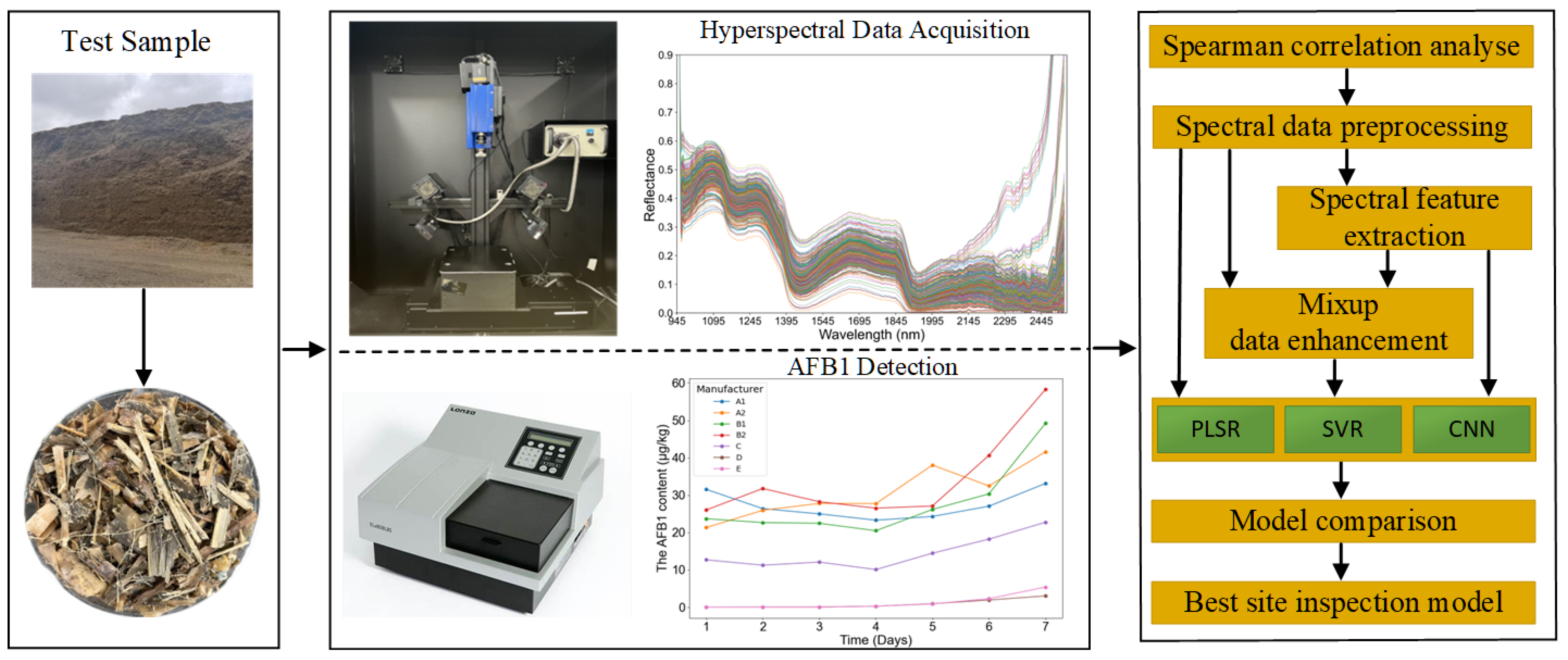
The main steps of sample collection and data analysis are illustrated in Figure 1. Specifically, this study focuses on the following objectives: (1) Investigate the feasibility of using hyperspectral imaging (HSI) technology for the quantitative analysis of AFB1 content in maize silage. (2) Apply nine data preprocessing methods, three feature wavelength selection techniques, and data augmentation method Mixup to obtain different spectral datasets, and using these datasets, construct and compare the performance of a linear model (PLSR), a nonlinear model (SVR), and a deep learning model (CNN), systematically evaluating the impact of different data processing approaches on model performance, identifying the most suitable dataset, and establishing corresponding base models. (3) Optimize the parameters and structures of the base models, compare the performance of PLSR, SVR, and CNN models, and select the optimal model with high accuracy and strong generalization ability for on-site detection.

2. Materials and Methods

The raw materials used in this study were collected from seven dairy farms located across three regions in the Inner Mongolia Autonomous Region of China. The farms were designated as follows: A1 and A2 in Baotou City (longitude 109°15′–110°26′ E, latitude 40°15′–42°43′ N); B1 and B2 in Liangcheng County, Ulanqab City (longitude 112°28′–112°30′ E, latitude 40°29′–40°32′ N); and C, D, and E in Hohhot City and Helingeer County (longitude 111°26′–112°18′ E, latitude 39°58′–40°41′ N). The maize varieties used at each location were as follows: “Baoyu 2307” in Baotou City, “Xiandai silag No.15” in Liangcheng County, and “Jingke silag 516” in Hohhot City and Helingeer County.

According to the standard full-plant maize silage process of Inner Mongolia Autonomous Region, maize was harvested at the stage when the kernel milk line reached approximately 66% (from the late milk stage to the early dough stage) and chopped into lengths of 10–20 mm. After chopping, the material was thoroughly mixed and packed into cement-structured silage bunkers. The filling was performed layer by layer, with each layer compacted to a thickness of 30–50 cm. Upon completion, the silage material extended approximately 30 cm above the bunker opening. During filling, fermentation additives could be sprayed to promote the proliferation of lactic acid bacteria. After compaction, a 10–20 cm layer of finely chopped straw was applied on the surface, followed by a plastic film cover and weighting with rubber tires. The bunker top was shaped into a dome to facilitate water runoff, and drainage ditches were constructed around the bunker to prevent water accumulation.

The silage was sealed and stored for 2–5 months before opening. During feed-out, the silage was removed along a cross-sectional plane perpendicular to the bunker wall, proceeding from top to bottom to avoid tunneling or full exposure of the silage face. It should be noted that certain operational parameters, including harvest timing, chopping length, and fermentation additive formulations, varied among farms due to proprietary technologies and are not disclosed in detail in this paper. All farms completed the silage preparation process in September 2023 and opened the silage bunkers in March 2024.

2.1. Sample Collection

The experimental materials were sourced from dairy farms of three different scales: large, medium, and small. The experimental period was divided into five stages.

The first stage included manufacturers A1 and A2, located in Baotou City (medim-sized dairy farms), with the experimental period from 15 April to 25 April 2024.The second stage involved manufacturers B1 and B2, located in Liangcheng county of Wulanchabu City and (small-sized dairy farms), with the experimental period from 30 April to 9 May 2024. The third, fourth, and fifth stages covered manufacturers C, D, and E, located in Helingeer county of Hohhot City (large-scale dairy farms), with the experimental periods from 27 May to 5 June, 7 June to 19 June, and 24 June to 3 July 2024, respectively.

During on-farm sampling, adult dairy cows were fed 2–3 times daily, and samples were collected during the first feeding of the day. Sampling points were selected based on the center of the silage pit cross-section, combined with equidistant points vertically and horizontally, to ensure the representativeness and uniformity of the samples. The collected silage samples were immediately sealed in specialized silage bags, preserved with ice packs, and transported to the laboratory within approximately one hour.

Upon arrival at the laboratory, samples were subdivided according to manufacturer and stage: three portions per manufacturer for the first and second stages, and six portions per manufacturer for the third to fifth stages. Each portion was tightly packed into polystyrene foam boxes with dimensions of 58 cm × 43 cm × 27.5 cm. Polystyrene foam boxes, widely used for the preservation of vegetables and seafood due to their excellent thermal insulation and moisture resistance, were selected to simulate actual silage storage conditions in the bunker silo.

To further simulate the secondary oxidation that may occur during on-farm sampling, the polystyrene foam boxes were covered with uniformly perforated aluminum foil and placed in a cool and ventilated area to undergo continuous aerobic exposure. The aerobic exposure period began on the day the samples arrived at the laboratory (designated as Day 0) and continued for 6 days, with sampling conducted daily at 8:00 AM. Sampling points included Day 0, Day 1, Day 2, Day 3, Day 4, Day 5, and Day 6. The sampling process remained consistent throughout to ensure data comparability and experimental repeatability.

During each sampling event, samples were collected on a per-manufacturer basis from the corresponding three polystyrene foam boxes. Each box was sampled evenly from both upper and lower layers, following a pattern from the center to the surrounding areas. A total of 500 g of silage was collected per sampling event. After thorough homogenization, the samples were reduced to 60 g ± 0.5 g using the quartering method [24]. Functional subsampling was then performed. A portion of 50 ± 0.5 g was placed in a Petri dish with a diameter of 10 cm and a height of 1 cm for visible and near-infrared spectroscopy (VIS-NIRS) data collection. A portion of 10 ± 0.5 g was sealed in a self-sealing bag for AFB1 content analysis.

2.2. AFB1 Detection

According to Technical Guidelines for Aflatoxin B1 Control in Maize Silage Feed for Dairy Farms, issued by the Ministry of Agriculture and Rural Affairs of China, this study used the PriboFast^® ELISA AFB1 Detection Kit (EKT_010_96T, Pribolab, Qingdao, China) to measure the AFB1 content in maize silage feed. The experiment was conducted at the Inner Mongolia Agricultural, Animal Husbandry and Fishery Biotechnology Research Center. The sample preparation process is as follows.

Preparation Washing Solution: dilute concentrated washing solution with deionized water at a 1:9 volume ratio.

60% Methanol Solution: dilute methanol solution with deionized water at a 3:2 volume ratio.

Sample processing: weigh 2.50 g of maize silage sample (PL_602L, 0.01 g precision), add 20 mL of 60% methanol solution, and homogenize using a high speed dispersion homogenizer for 30–45 s (FJ_200, Shanghai Huxi Industry Co., Ltd., Shanghai, China). Rinse the homogenizer head with 5 mL of 60% methanol solution into the centrifuge tube, and continue homogenizing. After homogenization, place the sample in a constant temperature shaker for 5 min (ZHWY_200D, Shanghai Zhicheng Analytical Instrument Manufacturing Co., Ltd., Shanghai, China). Centrifuge the sample at 4000 rpm for 5 min using a low temperature high speed centrifuge (LEGEND MACH1.6R, ThermoFisher, Shanghai, China) to obtain the maize silage feed filtrate.

AFB1 Content Measurement: mix 200 μL of filtrate with 300 μL of sample diluent I, adjust the pH to 6.0–8.0, and mix thoroughly to prepare the sample for testing. Add 50 μL of the prepared sample to each well of the microplate (EKT_010_96T, Pribolab, Qingdao, China), with 2 replicate wells per sample. Add enzyme label solution and antibody reagent solution in sequence and incubate for 30 min. Wash the wells 3–4 times, then add the chromogenic reagent and incubate for 15 min. Add stop solution to terminate the reaction, and absorbance was measured at 450 nm using a microplate reader (ELX808, ThermoFisher, Shanghai, China). Finally, calculate the AFB1 content based on the absorbance.

2.3. Hyperspectral Data Acquisition

The hyperspectral equipment used in this study was the WuLing Optics Hyperspectral Imaging System (Isuzu Optics, Taiwan, China). The system includes both visible and near-infrared (NIR) spectral components, with this study primarily utilizing the NIR spectral system for data acquisition. The system has a wavelength range of 935–2539 nm, a spectral resolution of 8 nm, and a total of 256 spectral bands. The main components of the system include a hyperspectral image spectrometer (ImSpector Model N25E, Spectral Imaging Ltd., Oulu, Finland), a CCD camera (Xeva_FPA_2.5_320, Xenics Ltd., Leuven, Belgium), six halogen lamps (arranged in two groups of three 50 W lamps each) (DECOSTAR^® 51 STANDARD, OSRAM Ltd., Munich, Germany), a mobile control platform (IRCP0076_1COM, ISUZU Optics Co., Ltd., Taiwan, China), and a computer. The motorized translation stage operates at a movement speed of 20.38 mm/s, with a camera exposure time of 2.16 ms. The scanning area covers an actual length of 180 mm and width of 80 mm. The entire system is housed in a dark chamber to minimize external light interference. The distance between the sample Petri dish surface and the camera lens was set at 45.5 mm.

Due to the uneven intensity distribution across different spectral bands and the interference of dark current in the camera, the raw hyperspectral images contain substantial noise. To correct this, the built-in software of the hyperspectral imaging system was used for data calibration using white reference and dark reference corrections [24]. The image correction formula is as follows:

$$\mathrm{R}={\displaystyle \frac{{\mathrm{R}}_{\mathrm{r}\mathrm{a}\mathrm{w}}-{\mathrm{R}}_{\mathrm{d}\mathrm{a}\mathrm{r}\mathrm{k}}}{{\mathrm{R}}_{\mathrm{w}\mathrm{h}\mathrm{i}\mathrm{t}\mathrm{e}}-{\mathrm{R}}_{\mathrm{d}\mathrm{a}\mathrm{r}\mathrm{k}}}}$$

(1)

where R is the corrected hyperspectral image, ${\mathrm{R}}_{\mathrm{r}\mathrm{a}\mathrm{w}}$ is the raw hyperspectral image, ${\mathrm{R}}_{\mathrm{w}\mathrm{h}\mathrm{i}\mathrm{t}\mathrm{e}}$ is the white reference image, obtained using white Teflon with a reflectance of 99%. ${\mathrm{R}}_{\mathrm{d}\mathrm{a}\mathrm{r}\mathrm{k}}$ is the dark reference image, obtained by turning off the light source and completely covering the lens with a black cap. To reduce background noise and dark current interference from the camera, the near-infrared spectrometer system was calibrated using a standard white reference panel and a lens cap before acquiring hyperspectral imaging data for maize silage, following the correction formula.

To ensure the systematic and representative collection of data, this study implemented a staged sampling strategy based on different manufacturers. In the first stage (manufacturers A1 and A2) and the second stage (manufacturers B1 and B2), each manufacturer collected 3 samples per day. In the third stage (manufacturer C), fourth stage (manufacturer D), and fifth stage (manufacturer E), each manufacturer collected 6 samples per day. For each sample, two sets of spectral data were acquired: after completing the first acquisition, the sample was thoroughly shaken and flipped before performing the second acquisition, in order to improve the uniformity and reliability of the spectral data. Each trial was conducted over a continuous period of 7 days.

As a result, manufacturers A1, A2, B1, and B2 each obtained 42 spectral datasets, totaling 168 datasets across the four manufacturers. Manufacturers C, D, and E each collected 84 spectral datasets, totaling 252 datasets across these three manufacturers. In summary, a total of 420 spectral datasets were collected in this study, providing sufficient data support for subsequent model training and performance analysis.

2.4. Spectral Data Extraction

A program was developed using Python 3.8 and PyTorch 1.10.1 to extract the region of interest (ROI) from the corrected hyperspectral images. The ROI was centered in the image with a size of 130 × 130 pixels, capturing the average spectral data of maize silage components, which is a random combination of straw, stems and leaves, maize kernels, maize cobs, and other background elements.

The near-infrared spectral system recorded 256 spectral bands within the 935–2539 nm wavelength range. After removing three abnormal variables, a total of 253 spectral bands were retained. The final dataset comprised 420 spectral data points, with a total of 106,260 spectral reflectance values.

2.5. Analysis of Variance

Analysis of variance (ANOVA) is a statistical method used to determine whether there are significant differences between the means of different groups [25]. Its principle is to compare the between group variance and within-group variance to assess whether there are significant differences in the data from different groups. Key evaluation metrics of ANOVA include the F-value (the ratio of between group variance to within-group variance, where a larger F-value indicates a more significant difference between groups) and the p-value (used to determine whether the null hypothesis is rejected; typically, when the p-value < 0.05, the result is considered significant, and the null hypothesis is rejected).

2.6. Spearman’s Correlation Analysis

Spearman’s correlation analysis is a non-parametric statistical method, suitable for measuring nonlinear relationships or cases with outliers in the data [26]. The principle is to rank the data, calculate the squared differences in ranks, and then obtain the correlation coefficient. Spearman’s correlation coefficient ranges from −1 to +1, where +1 indicates perfect positive correlation, −1 indicates perfect negative correlation, and 0 indicates no correlation. The main evaluation metric of Spearman’s analysis is the correlation coefficient, and the closer the value is to ±1, the stronger the monotonic relationship between the variables.

2.7. Spectral Preprocessing

During hyperspectral image acquisition, factors such as instrument noise, dark current, environmental conditions, and the irregular surface of maize silage samples can cause baseline drift, spectral overlap, and a low signal-to-noise ratio, thereby affecting the model’s interpretability. To address these challenges, various spectral preprocessing techniques were applied: Savitzky–Golay (SG) smoothing, which fits a polynomial within a moving window to smooth the data, reducing noise while preserving key signal features. Standard Normal Variate (SNV), which standardizes the spectral data of each sample to eliminate baseline drift and amplitude variations caused by scattering effects or particle size differences, making sample comparisons more consistent and reliable. Multiplicative Scatter Correction (MSC), which corrects baseline drift and amplitude variations in spectral samples to reduce spectral variations caused by scattering effects and particle size differences, ensuring spectral consistency. The First Derivative (FD) calculates the rate of change in spectral data to emphasize rapidly changing regions in the spectrum, enhancing spectral details, eliminating baseline drift, and improving signal resolution. The Second Derivative (SD) computes the second derivative of the spectral curve to highlight details of absorption peaks and curvature variations while reducing background signals and noise. This study applies SG, SNV, MSC, FD, and SD, as well as combined preprocessing methods including SNV + FD, MSC + FD, SNV + SD, and MSC + SD to identify the optimal spectral preprocessing approach for AFB1 detection in maize silage [25,27,28,29].

2.8. Feature Spectral Selection

Feature selection is the process of selecting a subset of input features without altering the original data. Its objective is to iteratively optimize a target function and identify the optimal feature subset from all possible combinations through an appropriate search strategy, thereby enhancing model performance.

Competitive Adaptive Reweighted Sampling (CARS) is a feature selection method based on the Partial Least Squares (PLS) regression model. Using an Adaptive Reweighted Sampling (ARS) strategy, CARS iteratively retains variables with larger absolute regression coefficients while gradually eliminating redundant information. The subset of variables that yields the lowest root mean square error of cross-validation (RMSECV) is ultimately selected as the optimal set of feature wavelengths.

Bootstrapping Soft Shrinkage (BOSS) integrates bootstrapping and soft shrinkage techniques. BOSS first applies bootstrapping to resample from the original dataset multiple times, generating various data subsets. Then, soft shrinkage is applied to adjust variable coefficients, reducing noise while preserving the most informative spectral features.

Random Forest (RF) evaluates the contribution of different features within a model and selects the most influential ones for prediction, thereby optimizing model performance.

This study attempts to use CARS (Competitive Adaptive Reweighted Sampling), BOSS (Bootstrapping Soft Shrinkage), and RF (Random Forest) methods to select feature wavelengths from the hyperspectral data of AFB1 in maize silage [30,31,32].

2.9. Mixup Data Augmentation

Data Augmentation is a method that generates new samples by transforming the original data, aiming to increase the diversity and quantity of the dataset. This approach helps the model learn more features, reduces overfitting, and effectively enhances the model’s generalization ability and robustness [33]. In this study, the Mixup data augmentation method was used to perform interpolation between the original samples and randomly selected samples, generating new augmented samples. Specifically, a Beta distribution is first used to generate a weighting coefficient for each sample, which determines the proportion of the original sample and the randomly selected sample in the weighted combination. Then, this weighting coefficient is applied to mix the spectral data and corresponding target variables of the original and randomly selected samples, generating new augmented spectral data. Mixup generates augmented samples from two or more examples, leading to multiple labels that better reflect real world conditions [34].

2.10. Models and Evaluation

Chemometric methods are an essential component of near-infrared spectroscopy analysis. Currently, the most commonly used linear and nonlinear quantitative models are partial least squares regression (PLSR) and Support Vector Regression (SVR), respectively. Convolutional Neural Networks (CNNs) represent an emerging technology in the field of non-destructive quality detection of agricultural products. However, in the domain of AFB1 detection in maize silage using near-infrared spectroscopy, these methods have yet to be explored.

This study constructed three predictive models: PLSR, SVR, and CNN to explore the relationship between hyperspectral near-infrared spectroscopy and AFB1 content in maize silage and to identify the optimal on-site detection model. PLSR, a commonly used multivariate linear regression method in hyperspectral modeling, projects the original spectral data into a latent variable (LV) space and constructs a regression model based on the optimal number of LVs, effectively addressing high-dimensional data and multicollinearity issues [35]. In contrast, SVR, a nonlinear regression method, balances model complexity and prediction error by minimizing their weighted sum, thereby enhancing both model accuracy and generalization capability, optimizing the regression performance of hyperspectral data [36].

CNN utilizes automatic feature extraction and parameter sharing in convolutional layers to reduce computational complexity and the number of parameters, improving training efficiency and generalization [37]. To further enhance the model’s performance, CAM, SE, SA, CBAM, and Transformer attention mechanism modules were sequentially introduced into the CNN model. Covariance Attention Mechanism (CAM) captures cross-feature correlations through the covariance matrix [38]. The Squeeze and Excitation Attention Mechanism (SE) is a lightweight channel attention mechanism that dynamically learns the importance weights of each channel, thereby enhancing feature representation [39]. The Spatial Attention Mechanism (SA) focuses on spatial information and captures important regions in the spatial dimension of feature maps, improving the model’s ability to focus on critical areas [40]. Convolutional Block Attention Module (CBAM) combines channel and spatial attention mechanisms to further enhance feature representation, Transformer captures the global dependencies between elements at different positions in the input sequence, effectively modeling long range dependencies [41].

The model performance evaluation metrics include the coefficient of determination (R²), root mean square error (RMSE), and residual predictive deviation (RPD). These metrics are used to assess both the training and testing sets, including the coefficient of determination (${\mathrm{R}}_{\mathrm{C}}^2$) and root mean square error of calibration (RMSEC) for the training set, as well as the coefficient of determination (${\mathrm{R}}_{\mathrm{P}}^2$), root mean square error of prediction (RMSEP), and residual predictive deviation (RPD) for the testing set [42].The coefficient of determination (R²) measures how well the model explains the variability in the samples, with values closer to 1 indicating better explanatory power. The root mean square error (RMSE) quantifies the difference between predicted and actual values, with lower RMSE indicating higher prediction accuracy. The residual predictive deviation (RPD) is used to evaluate model performance: an RPD below 1.5 indicates poor performance, a value between 1.5 and 2.5 suggests moderate performance, an RPD between 2.5 and 3.0 is considered good, and an RPD above 3.0 represents an excellent model.

3. Results

3.1. AFB1 Content Analysis

The Technical Guidelines for Aflatoxin Prevention and Control in Maize Silage for Dairy Farms issued by the Ministry of Agriculture and Rural Affairs of China set the AFB1 limit for whole plant maize silage for lactating cows at ≤30 μg/kg, with a warning threshold of 21 μg/kg. For TMR (Total Mixed Ration) for lactating cows, the AFB1 limit is ≤15 μg/kg, with a warning threshold of 10.5 μg/kg. The guidelines recommend that farms conduct AFB1 testing in maize silage and TMR for lactating cows every two weeks in the spring and every week in the summer and autumn. If the AFB1 content in maize silage exceeds the limit, it is prohibited to feed it to lactating cows; if it exceeds the warning threshold, fungal toxin binders should be used, the formula adjusted, the amount of maize silage reduced, or the fungal toxin content diluted before feeding. When the content is below the warning threshold, it can be fed normally.

The Inner Mongolia local standard DB15/T956-2022 [43] Whole Plant Maize Silage Quality Evaluation classifies maize silage quality based on the total score: 85–100 points is classified as Grade 1, 70–84 points as Grade 2, <70 points as Grade 3, and <60 points as unqualified. The evaluation indicators include sensory (10 points), nutritional components (45 points), fermentation quality (35 points), and hygienic quality (10 points). In the hygienic quality section (10 points), AFB1 content of ≤1 μg/kg earns 5 points, 1–4 μg/kg (including 4) earns 3 points, and 4–30 μg/kg (including 30) earns 1 point.

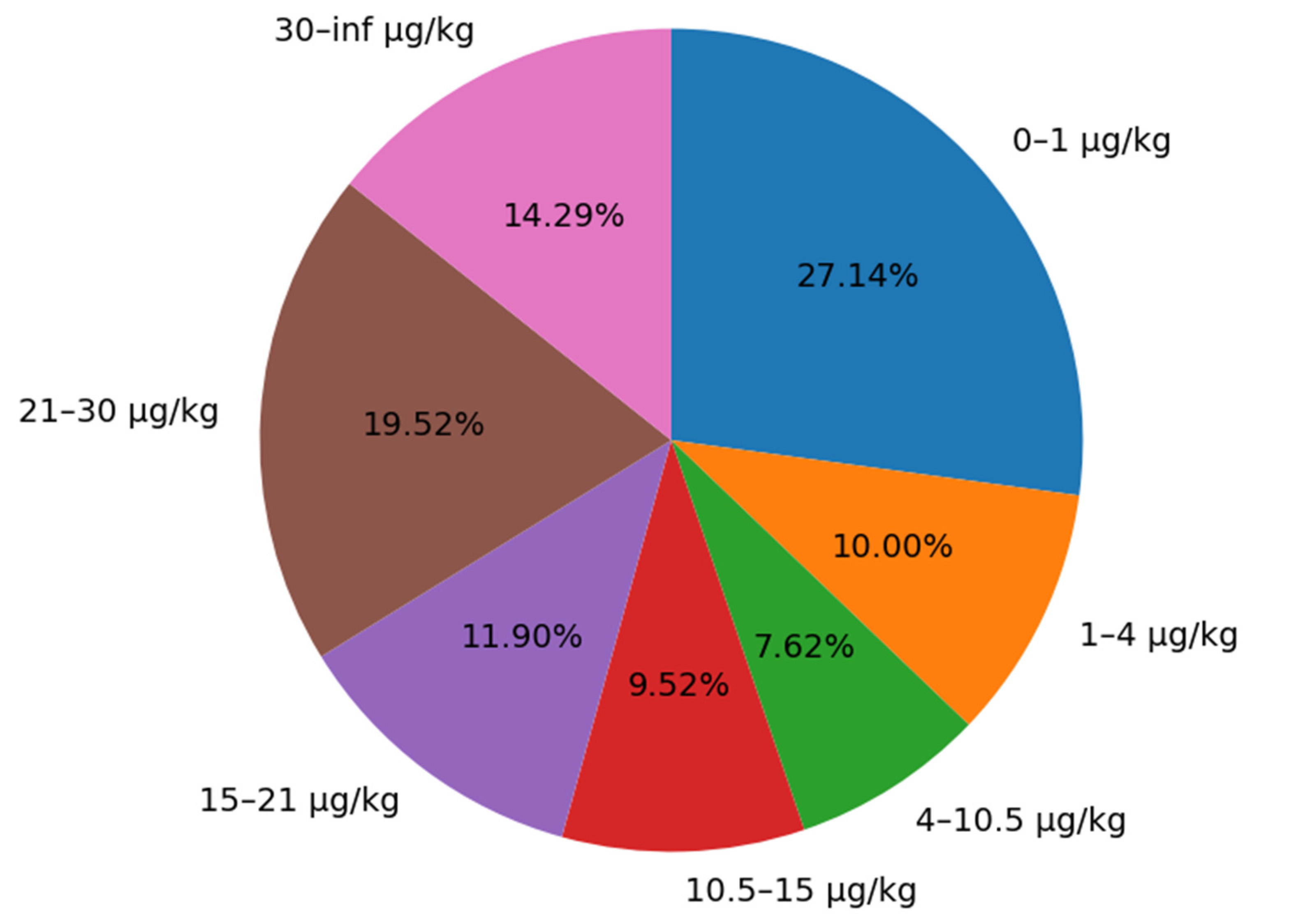
This study divides the AFB1 content data of maize silage into the following intervals: 0–1 μg/kg, 1–4 μg/kg, 4–10.5 μg/kg, 10.5–15 μg/kg, 15–21 μg/kg, 21–30 μg/kg, >30 μg/kg. The goal is to show that the data collected in the experiment covers the relevant limits and warning values for AFB1 in whole plant maize silage as defined by China and the Inner Mongolia Autonomous Region. The sample proportions for each interval are shown in Figure 2.

From the data distribution, the sample proportions for each range are as follows: 0–1 µg/kg (27.14%), 1–4 µg/kg (10.00%), 4–10.5 µg/kg (7.62%), 10.5–15 µg/kg (9.52%), 15–21 µg/kg (11.90%), 21–30 µg/kg (19.52%), and >30 µg/kg (14.29%). The distribution of AFB1 levels in this study is relatively balanced, covering samples with different range levels, thereby accurately reflecting the current contamination status of AFB1 in maize silage and ensuring the representativeness of the dataset.

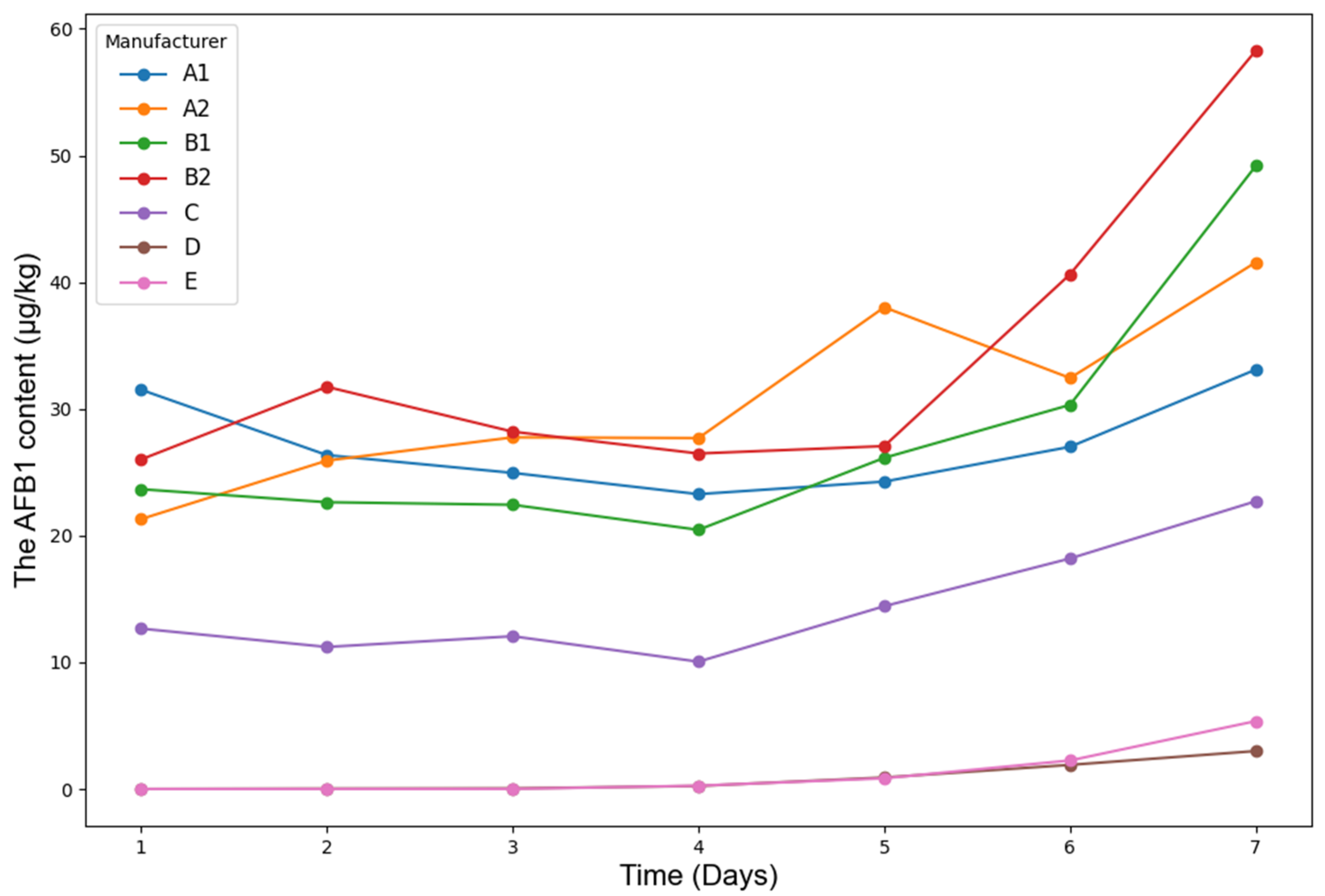
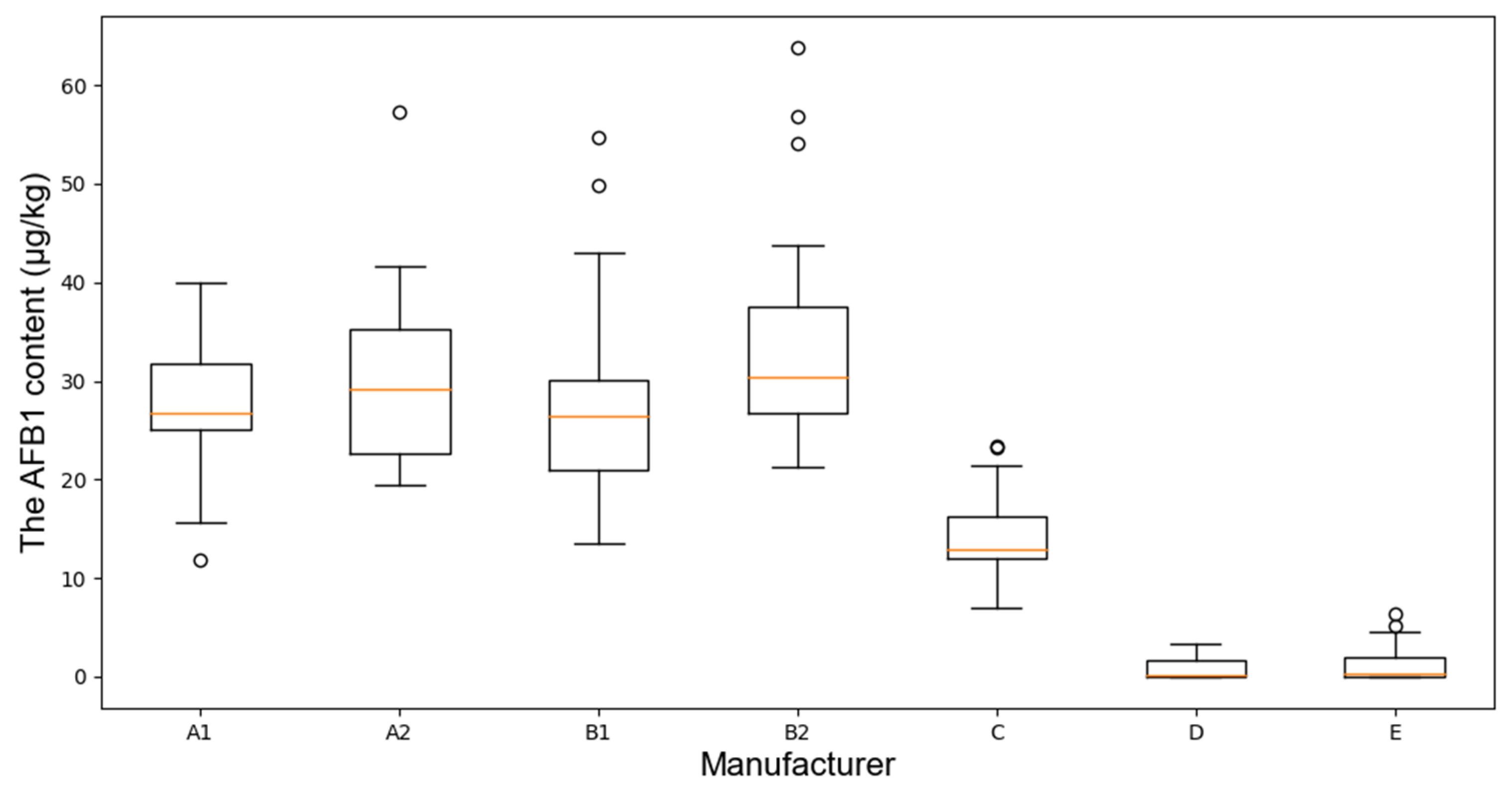
Under identical experimental conditions, Figure 3 presents the temporal variation trend of AFB1 content in maize silage from different manufacturers, while Figure 4 illustrates the variation range of AFB1 content across manufacturers.

As shown in Figure 3, the AFB1 content in maize silage from manufacturers A1, A2, B1, B2, C, D, and E exhibited an overall increasing trend over time, with a marked acceleration observed after Day 5. Notably, A1, A2, B1, and B2 demonstrated a more rapid rise in AFB1 levels, indicating that their raw materials may be more susceptible to mold contamination. In contrast, C, D, and E showed a relatively stable increase, suggesting stronger resistance to mold proliferation.

According to the fluctuation range analysis in Figure 4, A1 and A2 displayed greater variability in AFB1 content, with A1 showing a lower overall distribution, which may be attributed to inconsistent raw materials or storage conditions. B1 and B2 showed smaller fluctuations, but the presence of outliers indicates potential instability in storage or processing procedures. In comparison, C, D, and E exhibited lower AFB1 concentrations with more concentrated distributions, implying that their storage environments were more stable and effective in suppressing AFB1 production.

The time-dependent trends and fluctuation ranges of AFB1 data provide valuable insights for the development of non-destructive detection models. The temporal dynamics enhance the model’s capability to predict AFB1 variation patterns over time. Moreover, the observed differences in AFB1 growth behaviors among manufacturers contribute to data diversity, which is crucial for improving the generalization performance of the models.

3.2. Raw Spectral Analysis

The raw spectra of maize silage samples are shown in Figure 5, covering the wavelength range of 935–2539 nm. The spectral curves indicate that samples with different AFB1 concentrations exhibit variations in absorbance at different wavelengths. Peak values are observed at 1120 nm, 1280 nm, 1650 nm, and 1870 nm, while valleys appear at 1188 nm, 1447 nm, and 1990 nm. These absorption wavelengths correspond to the stretching or vibrational modes of C-C, C-O, and C-H chemical bonds.

Additionally, reflectance outliers in the 2250–2450 nm range align with the outlier trends in the box plot, suggesting that this spectral region may be influenced by moisture and matrix effects. Based on previous studies, these characteristic wavelengths are likely associated with moisture, starch, proteins, and fungal metabolites, providing a fundamental theoretical basis for using hyperspectral technology to predict AFB1 content.

3.3. Analysis of Variance

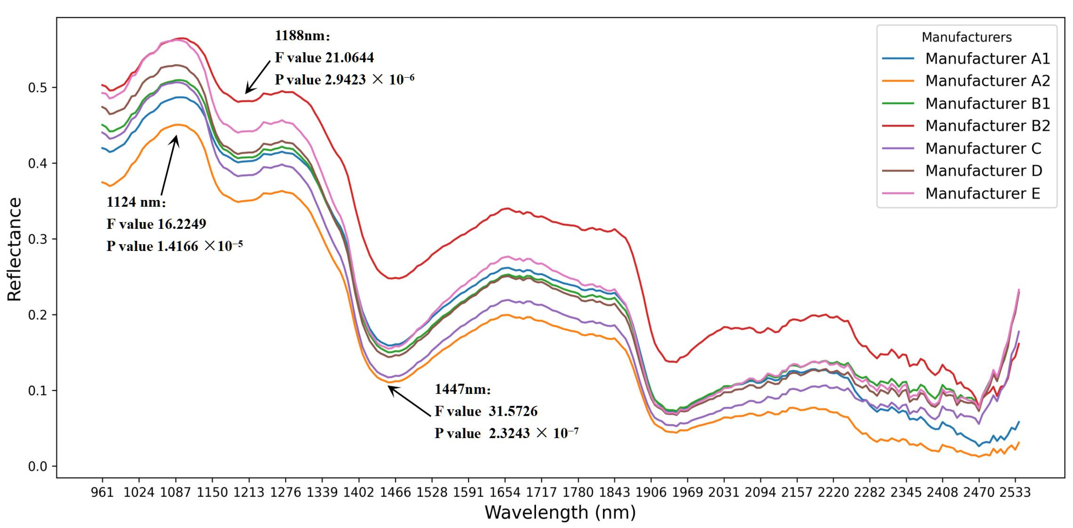
To further explore the relationship between spectral data and AFB1 content in maize silage, a statistical analysis was conducted on the sample spectral data Figure 6 presents the average spectral data collected on Day 4 from different manufacturers, and a one way analysis of variance (ANOVA) was performed to evaluate spectral differences among samples.

The results indicate that at 1124 nm (F = 16.2249, p = 1.4166 × 10⁻⁵), 1188 nm (F = 21.0644, p = 2.9423 × 10⁻⁶), and 1447 nm (F = 31.5726, p = 2.3243 × 10⁻⁷), the spectral reflectance exhibited significant differences among samples (p < 0.01). This finding suggests that spectral characteristics vary among samples during the mold contamination process, providing a theoretical basis for non-destructive AFB1 detection using hyperspectral data.

3.4. Spearman Correlation Analysis

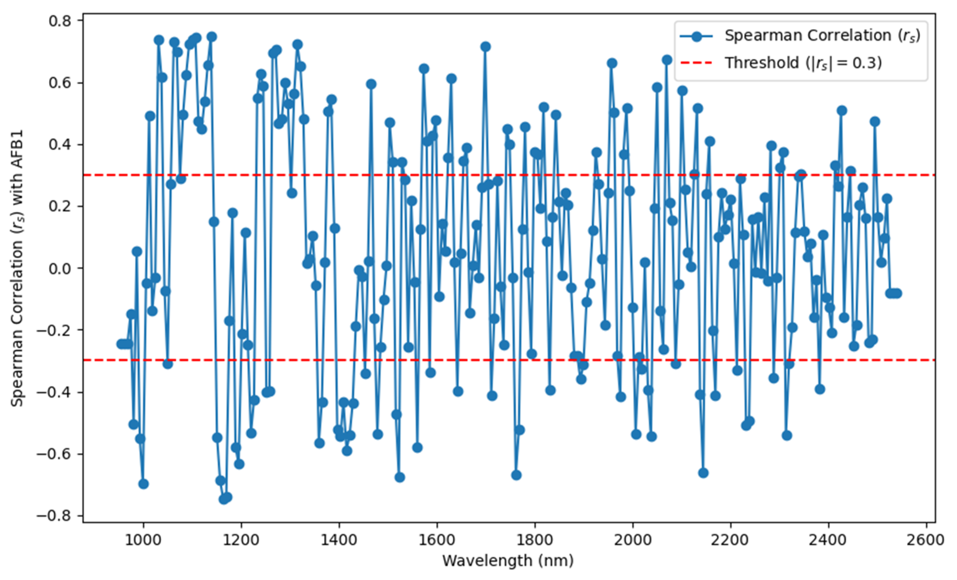
To further validate the feasibility of hyperspectral data for non-destructive AFB1 detection, this study employed Spearman’s correlation analysis to calculate the relationship between spectral reflectance and AFB1 content, with the results presented in Figure 7. The analysis indicates that within the 935–2539 nm wavelength range, approximately 47.43% (120 wavelengths) exhibited a significant correlation with AFB1 content (|${\mathrm{r}}_{\mathrm{s}}$| ≥ 0.3), with the highest correlation observed at 1137.62 nm (|${\mathrm{r}}_{\mathrm{s}}$| = 0.7480). Additionally, multiple wavelengths, such as 979.74 nm, 998.69 nm, 1030.28 nm, and 2445.27 nm, demonstrated stable correlations across different spectral regions, further confirming that near-infrared hyperspectral data effectively characterize AFB1 content variations.

3.5. Dataset Splitting

The Kennard-Stone algorithm [44] was employed to divide the modeling dataset into a training set and a test set at an 8:2 ratio. To ensure reproducibility, the parameter random_state = 42 was set, while shuffle = True was enabled to enhance data randomness. To improve model stability, the dataset underwent standardization, where the data were mean centered and scaled to unit variance. As shown in

Table 1. Descriptive Statistics of AFB1 Mycotoxin Content in maize Silage Samples.

Sample Sets	Sample Number	Maximum (μg·kg⁻¹)	Minimum (μg·kg⁻¹)	Mean (μg·kg⁻¹)	Standard Deviation (μg·kg⁻¹)
Calibration set	672	68.3008	0	15.0088	14.1626
Prediction set	168	68.3008	0	14.8532	13.4721

, the maximum and minimum AFB1 values in the test set are consistent with those in the training set, while the mean and standard deviation are also similar. This indicates a balanced data distribution with no significant bias, thereby enhancing the model’s generalization capability.

3.6. Spectral Preprocessing

The raw spectral data, along with data processed using various preprocessing methods (SG, SNV, MSC, FD, SD, as well as combined methods SNV + FD, MSC + FD, SNV + SD, MSC + SD) were separately input into the PLSR, SVR, and CNN models. The results are shown in

Table 2. Chemometrics results of the PLS, SVR, and CNN model for AFB1-contaminated samples analyzed with different preprocessing methods.

Model	Preprocessing Method	Calibration		Prediction
		${\mathbf{R}}_{\mathbf{C}}^2$	RMSEC	${\mathbf{R}}_{\mathbf{P}}^2$	RMSEP	RPD
PLSR	SD	0.9013	4.4191	0.7277	7.9898	1.9163
	MSC + SD	0.9035	4.3683	0.7193	8.1123	1.8873
	FD	0.9004	4.4381	0.7185	8.1239	1.8846
	SNV + SD	0.9036	4.3660	0.7181	8.1287	1.8835
	SNV + FD	0.9098	4.2247	0.7035	8.3364	1.8366
	MSC + FD	0.9092	4.2379	0.7013	8.3676	1.8297
	MSC	0.9111	4.1937	0.6876	8.5573	1.7892
	SG	0.8942	4.5747	0.6804	8.6550	1.7690
	RAW	0.9059	4.3134	0.6761	8.7139	1.7570
	SNV	0.8876	4.7148	0.6726	8.7609	1.7476
SVR	SD	0.7620	6.8612	0.6596	8.9321	1.7141
	SNV + SD	0.7555	6.9534	0.6340	9.2622	1.6530
	MSC + SD	0.7550	6.9611	0.6332	9.2720	1.6512
	FD	0.6458	8.3701	0.6318	9.2908	1.6479
	RAW	0.4305	10.6129	0.6231	9.3996	1.6288
	SG	0.4285	10.6316	0.6175	9.4684	1.6170
	MSC + FD	0.6066	8.8212	0.5477	10.2972	1.4868
	SNV + FD	0.6080	8.8050	0.5471	10.3037	1.4859
	MSC	0.4536	10.3962	0.3785	12.0704	1.2684
	SNV	0.4841	10.1014	0.3775	12.0793	1.2675
CNN	SD	0.9242	4.0927	0.6888	8.3112	1.7925
	FD	0.8449	3.8707	0.6769	8.5416	1.7593
	SNV + SD	0.8216	5.5382	0.6658	8.7024	1.7298
	SG	0.8220	5.9405	0.6477	8.8511	1.6849
	SNV + FD	0.8143	5.9336	0.6444	9.0868	1.6770
	RAW	0.8094	6.0601	0.6315	9.1297	1.6473
	MSC + FD	0.7898	6.1405	0.6271	9.2942	1.6376
	MSC + SD	0.8548	6.4476	0.6214	9.3492	1.6251
	MSC	0.8228	5.3592	0.6213	9.4211	1.6251
	SNV	0.8257	5.9196	0.5989	9.4214	1.5790

. Using the test set ${\mathrm{R}}_{\mathrm{P}}^2$ as the evaluation criterion for preprocessing methods, the SD demonstrated the best performance across PLSR, SVR, and CNN models.

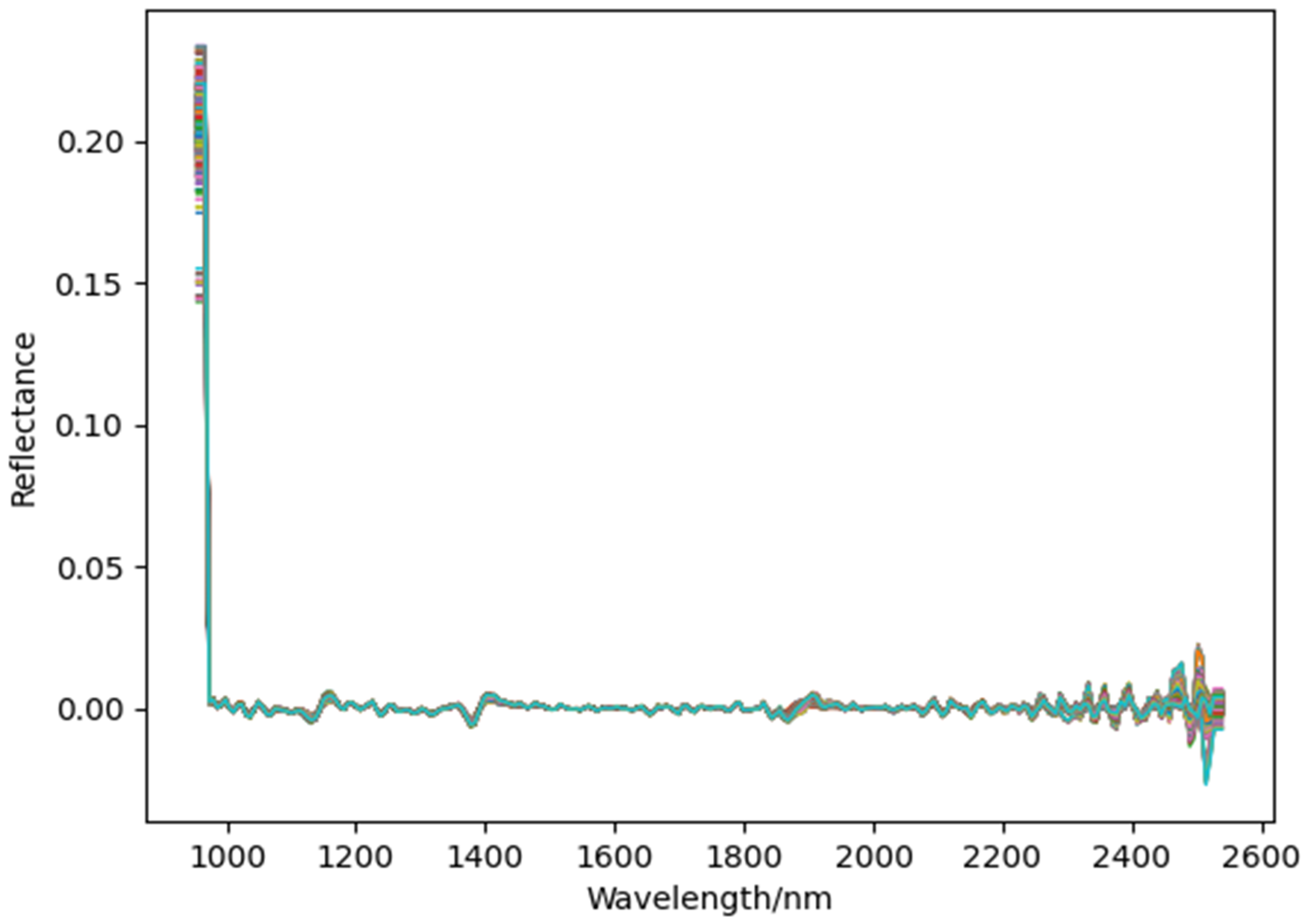
The spectral data after SD preprocessing is shown in Figure 8. Compared to the raw spectral data, the preprocessed spectra appear smoother and more tightly clustered, indicating that the SD preprocessing method effectively removes noise from the AFB1 spectral data in maize silage.

3.7. Comparative Analysis of Model Performance Based on Different Spectral Features

In this study, the spectral features of maize silage were derived from the full spectrum reflectance after SD preprocessing and the selected spectral bands based on CARS, BOSS, and RF feature selection methods. Linear PLSR, nonlinear SVR, and deep learning CNN models were built to predict AFB1 content.

In the construction of the PLSR model, GridSearchCV was used to search for the optimal number of principal components (n_components), with ${\mathrm{R}}_{\mathrm{P}}^2$ as the scoring metric. The final choice for n_components was 48, and 5-fold cross-validation (cv) was applied. In the construction of the SVR model, GridSearchCV was used to search for the optimal combination of hyperparameters C, epsilon, and kernel, with ${\mathrm{R}}_{\mathrm{p}}^2$ as the selection criterion for the best hyperparameters. The optimal combination was C = 100, epsilon = 0.2, and kernel = rbf, with 5-old cross-validation applied. The CNN model consisted of 6 convolutional layers, 3 pooling layers, and 5 normalization layers. ReLu activation functions were applied after each convolutional layer to enhance the model’s nonlinear capability. The output prediction was produced through a fully connected layer. The model was trained for 100 iterations using the MSE loss function and the Adam optimizer.

The prediction performance of the PLSR, SVR, and CNN models for AFB1 content in maize silage, based on the optimal parameters, is shown in

Table 3. Results of AFB1 Prediction Models for Maize Silage Based on Different Wavelengths.

Model	Extraction Method	Calibration		Prediction
		${\mathbf{R}}_{\mathbf{c}}^2$	RMSEC	${\mathbf{R}}_{\mathbf{p}}^2$	RMSEP	RPD
PLSR	/	0.9013	4.4191	0.7277	7.9898	1.9163
	CARS	0.9211	3.9505	0.7730	7.2942	2.0990
	BOSS	0.9190	4.0034	0.7294	7.9640	1.9224
	RF	0.8151	6.0469	0.6585	8.9466	1.7113
SVR	/	0.7620	6.8612	0.6596	8.9321	1.7141
	BOSS	0.9558	2.9546	0.8654	5.6174	2.7253
	CARS	0.9518	3.0870	0.8583	5.7635	2.6562
	RF	0.9130	4.1462	0.8268	6.3709	2.4030
CNN	/	0.9242	4.0927	0.6888	8.3112	1.7925
	BOSS	0.8225	5.9249	0.6513	9.0405	1.6935
	CARS	0.8326	5.7549	0.6354	9.2446	1.6561
	RF	0.8002	6.2856	0.6486	9.0759	1.6869

.

From the perspective of feature selection algorithms, the PLSR and SVR models built using feature wavelengths show significantly higher ${\mathrm{R}}_{\mathrm{p}}^2$ results in AFB1 prediction compared to their corresponding full wavelength models, indicating that feature selection methods have a significant impact on improving the performance of traditional machine learning models. Specifically, the PLSR_CARS model achieved a 6.2251% increase in ${\mathrm{R}}_{\mathrm{P}}^2$, an 8.7061% decrease in RMSEP, and a 9.5340% increase in RPD compared to the PLSR_SD model. The SVR_BOSS model achieved a 31.2007% increase in ${\mathrm{R}}_{\mathrm{p}}^2$, a 37.1100% decrease in RMSEP, and a 58.9931% increase in RPD compared to the SVR_SD model. These results suggest that the BOSS and CARS feature selection methods greatly enhance the model’s prediction performance by selecting wavelengths with higher predictive power.

The CNN model built using feature wavelengths has lower ${\mathrm{R}}_{\mathrm{p}}^2$ results in AFB1 prediction compared to the full wavelength model. Specifically, the CNN_BOSS model showed a 5.4443% decrease in ${\mathrm{R}}_{\mathrm{p}}^2$, an 8.7750% increase in RMSEP, and a 5.5230% decrease in RPD compared to the CNN_SD model. This result indicates that, in CNN methods, performing feature engineering steps may not significantly improve prediction performance and could even lead to a certain degree of performance degradation. This may be related to the feature extraction ability of the CNN model itself and the relatively small sample size, which limited the effectiveness of feature selection in bringing sufficient improvements.

From the perspective of modeling methods, the SVR model in this study showed significantly better prediction accuracy than both the PLSR and CNN models, suggesting the existence of a nonlinear relationship between spectral reflectance and AFB1 content in maize silage. SVR by utilizing kernel functions, is able to effectively capture nonlinear relationships in the data, particularly well-suited for handling high dimensional and complex datasets. Specifically, when using the BOSS feature selection method, the SVR model achieved an ${\mathrm{R}}_{\mathrm{p}}^2$ of 0.9558, RMSEP of 2.9546, and RPD of 2.7253, indicating that the SVR model not only provides accurate predictions but also has strong generalization ability. In contrast, the PLSR model, as a linear regression model, performs well when there is a strong linear relationship in the data, but its modeling capability is limited when handling complex nonlinear relationships. In this study, although the PLSR model showed improvement when using the CARS feature selection method, it still could not match the performance of the SVR model, demonstrating the limitations of linear models when dealing with nonlinear data.

The CNN model theoretically has strong automatic feature extraction capabilities, especially in handling high dimensional data, where they can automatically identify complex patterns through convolutional layers. However, in this study, the performance of the CNN model did not exceed that of the SVR model. One possible reason for this is the relatively small sample size. Deep learning models typically require large amounts of data to effectively learn and extract features, and with insufficient data, the CNN model’s advantages may not be fully realized, resulting in lower-than-expected prediction accuracy.

In the field of non-destructive testing of agricultural products’ quality, models combining chemometrics and artificial intelligence algorithms need to meet certain engineering application standards. Typically, a prediction set’s ${\mathrm{R}}_{\mathrm{p}}^2$ should be greater than 0.9, and the RPD should be greater than 3 to meet the engineering application’s precision and reliability requirements. However, the three models in this study, SVR, PLSR, and CNN, did not meet this standard, indicating that there is still room for optimization in these models for engineering applications. Therefore, further improvements in data processing and model structure are necessary to enhance the models’ detection performance and explore the feasibility of traditional machine learning and deep learning methods in the engineering applications for AFB1 detection in maize silage.

3.8. Data Augmentation and Model Structure Optimization

To improve the performance of PLSR, SVR, and CNN models in the non-destructive detection of AFB1 in maize silage, this study focuses on two key aspects: data augmentation and model structure optimization. The objective is to further enhance model predictive capability and meet engineering application requirements.

Data Augmentation: the Mixup method was applied to augment spectral data after feature selection. For instance, CARS selected spectral data (108 bands) was expanded from 45,360 to 90,720 samples, yielding the CARS_Mixup dataset. Similarly, BOSS_selected data (197 bands) was expanded from 82,740 to 165,480 samples, resulting in the BOSS_Mixup dataset. SD_preprocessed spectral data (253 bands) was also expanded from 106,260 to 212,520 samples, forming the SD_Mixup dataset.

Machine Learning Model Optimization: the PLSR model was enhanced via weight adjustment, yielding the WPLSR model, and its hyperparameters were automatically optimized within a range of 5 to 30 (step size = 1). The number of cross-validation folds was increased from 5 to 15. Furthermore, quadratic polynomial expansion (QPE) was employed to improve nonlinear feature representation, resulting in the WPLSR_QPE model.

The SVR model was optimized through principal component analysis (PCA), selecting the top 100 principal components to build the SVR_PCA model.

A summary of the machine learning model improvements is presented in

Table 4. The AFB1 prediction results for maize silage using different machine learning model.

Model	Data	Calibration		Prediction
		${\mathbf{R}}_{\mathbf{c}}^2$	RMSEC	${\mathbf{R}}_{\mathbf{p}}^2$	RMSEP	RPD
WPLSR_QPE	CARS_ Mixup	0.9734	2.2870	0.8657	4.6065	2.7292
	SD_ Mixup	0.9963	0.8606	0.9278	3.6088	3.7220
SVR_PCA	BOSS_ Mixup	0.9995	0.3158	0.9316	3.4368	3.8234
	SD_ Mixup	0.9993	0.3761	0.9458	3.1259	4.2969

.

The loss function of the deep learning CNN model was replaced with Huber Loss (HL) and Weighted Mean Squared Error (WMSE), respectively. Experimental results demonstrated that WMSE yielded superior performance, leading to the construction of the CNN_WMSE model.

The AFB1 prediction results for maize silage using different loss functions for CNN model architectures in

Table 5. The AFB1 prediction results for maize silage using different loss functions for the CNN model.

Model	Data	Calibration		Prediction
		${\mathbf{R}}_{\mathbf{c}}^2$	RMSEC	${\mathbf{R}}_{\mathbf{p}}^2$	RMSEP	RPD
CNN_MSE	SD_ Mixup	0.9300	3.7440	0.8689	4.8637	2.7617
CNN_HL		0.8773	4.9567	0.7685	6.4624	2.0785
CNN_WMSE		0.9504	3.1510	0.8830	4.5936	2.9241

.

To further enhance its predictive capability, various attention mechanisms including CAM, SE, SA, CBAM, and Transformer were sequentially integrated into the CNN_WMSE model. Among these, the SA (Spatial Attention) mechanism achieved the best performance. The AFB1 prediction results for maize silage using different attention mechanisms for CNN_WMSE model in

Table 6. The AFB1 prediction results for maize silage using different attention mechanisms for CNN_WMSE model.

Model	Data	Calibration		Prediction
		${\mathbf{R}}_{\mathbf{c}}^2$	RMSEC	${\mathbf{R}}_{\mathbf{p}}^2$	RMSEP	RPD
CNN_WMSE_SA	SD_Mixup	0.9953	0.9735	0.9112	4.0032	3.3654
CNN_WMSE_CBAM		0.9780	2.0986	0.8984	4.2815	3.1372
CNN_WMSE_SE		0.9581	2.8972	0.8865	4.5482	2.9687
CNN_WMSE_Transformer		0.9213	3.9697	0.8402	5.3695	2.5015
CNN_WMSE_CAM		0.9085	4.2815	0.8281	5.5688	2.4120

. The AFB1 prediction results of maize silage using different CNN architectures are summarized in Table 6. Under the parameter settings of kernel_size = 7, padding = 3, and bias = False, the final CNN_SD_Mixup_WMSE_SA model achieved an ${\mathrm{R}}_{\mathrm{p}}^2$ of 0.9174, an RMSEP of 3.8609, and an RPD of 3.4790.

3.9. Optimal AFB1 Detection Model for Maize Silage

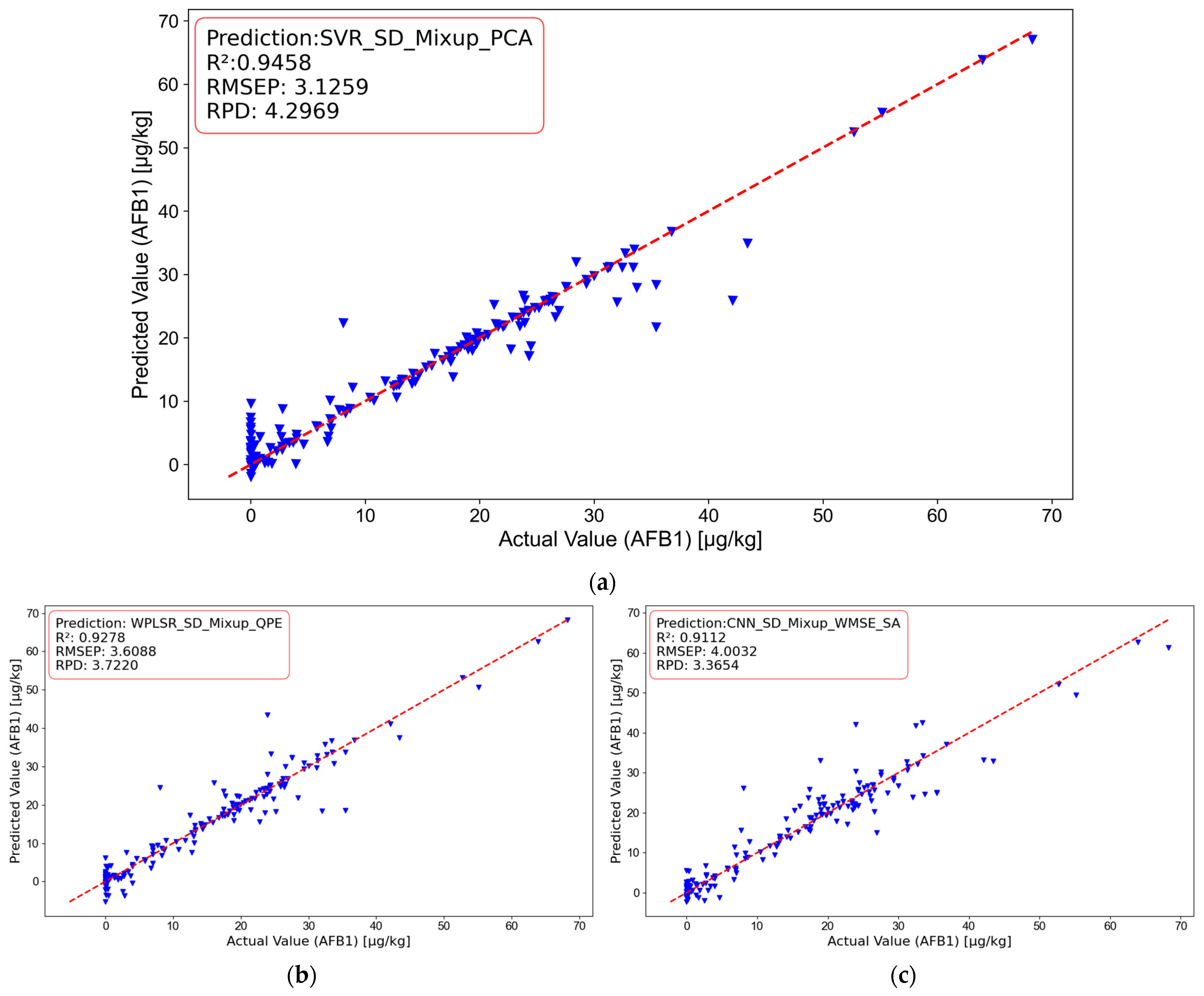
This study developed a non-destructive detection method for AFB1 in maize silage based on hyperspectral imaging technology. A comparison of the results obtained from different models is presented in

Table 7. The AFB1 best prediction results for different model on maize silage.

Model	Calibration		Prediction
	${\mathbf{R}}_{\mathbf{C}}^2$	RMSEC	${\mathbf{R}}_{\mathbf{P}}^2$	RMSEP	RPD
SVR_SD_Mixup_PCA	0.9993	0.3761	0.9458	3.1259	4.2969
WPLSR_SD_Mixup_QPE	0.9963	0.8606	0.9278	3.6088	3.7220
CNN_SD_Mixup_WMSE_SA	0.9953	0.9735	0.9112	4.0032	3.3654

. The best method is SVR_SD_Mixup_PCA method. The method achieved an ${\mathrm{R}}_{\mathrm{p}}^2$ of 0.9458, RMSEP of 3.1259, and RPD of 4.2969, with model evaluation metrics meeting the engineering application standards: ${\mathrm{R}}_{\mathrm{p}}^2$ > 0.9 and RPD > 3. Compared to the WPLSR_SD_Mixup_QPE method, SVR_SD_Mixup_PCA showed an improvement of 19.0315% in ${\mathrm{R}}_{\mathrm{p}}^2$, a reduction of 15.4484% in RMSEP, and an increase of 13.3797% in RPD. When compared to the CNN_SD_Mixup_WMSE_SA method, SVR_SD_Mixup_PCA showed an improvement of 36.5299% in ${\mathrm{R}}_{\mathrm{p}}^2$, a reduction of 28.0655% in RMSEP, and an increase of 21.6784% in RPD. These results indicate that the SVR_SD_Mixup_PCA method performs best for the non-destructive detection of AFB1 in maize silage. The regression plots of different model results are shown in Figure 9.

4. Discussion

The main innovations of this study include the following:

(1)

Exploring the feasibility of hyperspectral imaging (HSI) technology for the quantitative analysis of AFB1 content in maize silage feed, filling the technical gap in hyperspectral detection of AFB1 in maize silage feed.

(2)

In terms of processing near-infrared spectral data of maize silage feed, nine spectral preprocessing methods (SG, SNV, MSC, FD, SD, and their combinations) were applied to full spectrum reflectance, three feature selection methods (CARS, BOSS, RF) were used for the selection of spectral bands, and data augmentation (Mixup) was employed to expand the reflectance data. Linear PLSR models, nonlinear SVR models, and deep learning CNN models were built with these spectral features.

The study found that the SD preprocessing method performed the best in both machine learning and deep learning models, establishing SD as the optimal preprocessing method for near-infrared spectral features of maize silage feed AFB1.

The study also revealed that different models showed varying levels of adaptability to feature selection. PLSR performed best on features selected by CARS, SVR showed the best performance with features selected by BOSS, while CNN relied on global spectral features.

Furthermore, the study confirmed that the Mixup data augmentation method effectively improved model performance. The PLSR model performed better on the SD_Mixup dataset than on the CARS_Mixup dataset. The SVR model performed better on the SD_Mixup dataset than on the BOSS_Mixup dataset, and the CNN model showed better performance on the SD_Mixup dataset than on the SD dataset.

Overall, the SD_Mixup dataset significantly improved the predictive performance of both machine learning and deep learning models, and the Mixup data augmentation method significantly enhanced the diversity of AFB1 spectral data in maize silage, thereby contributing to improved model robustness and generalization.

(3)

This study explored the optimal nondestructive detection method SVR_SD_Mixup_PCA for AFB1 in maize silage by combining hyperspectral technology with machine learning, which provides a new feasible solution for the engineering application of nondestructive detection of AFB1 in maize silage.

The results of this study are not only consistent with existing findings in the field of AFB1 detection but also present some new insights. This study demonstrates the feasibility of non-destructive hyperspectral detection of AFB1 content in maize silage feed, and the results align with those of Kim (2023) [17], who utilized hyperspectral imaging combined with PLS_DA and SVR for aflatoxin classification in maize. Kim’s study concluded that SVR outperforms PLS_DA in classification performance, which is consistent with the results of this study, where the SVR model showed the best performance. However, Kim’s study focused solely on qualitative analysis and did not address quantitative detection of AFB1, whereas this study applied SVR combined with data augmentation methods to achieve quantitative detection of AFB1 in maize silage feed.

Regarding the impact of feature selection methods, Deng (2022) [45] investigated the effect of near-infrared spectral feature optimization on the quantitative detection of AFB1 in maize and found that the SVR model optimized by Particle Swarm Optimization with Combined Moving Window (PSO_CMW) performed the best, with an RMSEP of 3.5967 µg/kg, ${\mathrm{R}}_{\mathrm{p}}^2$ of 0.9707, and RPD of 5.7538. This conclusion is consistent with the results of this study, where the SVR model also showed the best performance. Specifically, in this study, the RMSEP of the SVR_SD_Mixup_PCA model was 3.1259 µg/kg, lower than the result found by Deng (2022) [45]; the ${\mathrm{R}}_{\mathrm{p}}^2$ was 0.9993, higher than Deng’s value; and the RPD was 4.2969, which was lower than Deng’s result. This improvement suggests that Mixup methods have enhanced the accuracy of the SVR model in detecting AFB1 in maize silage feed. The decrease in RPD could be related to the complex composition of maize silage feed, which presents greater challenges for the model during the learning process.

Currently, there is limited research on non-destructive AFB1 detection methods for maize silage feed. This study, based on hyperspectral imaging technology, combined linear (PLSR), nonlinear (SVR), and deep learning (CNN) models to explore high-precision and high-generalization non-destructive detection methods for AFB1 in maize silage feed. Although this study has made some progress, it still has limitations.

(1)

As there is currently a lack of relevant studies on hyperspectral detection of AFB1 content in maize silage, the optimal model developed in this study (SVR_SD_Mixup_PCA) cannot be directly compared with existing literature. Furthermore, to ensure consistency in experimental conditions, the data required for external validation will be collected in the future under the same conditions.

(2)

The study selected maize silage feed from seven manufacturers and three geographical regions of Inner Mongolia. The Inner Mongolia Autonomous Region serves as a major base for agricultural and livestock production and processing in China. Statistical data indicate that more than one in every six cups of milk nationwide originates from this region, underscoring its critical role in the country’s dairy industry. The region hosts a large number of dairy farms, where maize silage is widely used as the primary feed, playing an essential role in supporting the nutritional requirements of dairy cattle and sustaining high milk production levels. But the total sample size remains relatively small, which affects the generalization ability of the model. Future research should expand the sample sources to improve the model’s adaptability.

(3)

In the early stages of maize silage spoilage, changes in internal material properties occur before visible alterations, making hyperspectral imaging particularly effective for early detection. As spoilage progresses, external characteristics such as color, texture, and shape also change. Although this study did not incorporate appearance image data, future research could explore multimodal approaches that integrate both spectral and visual information.

(4)

The deep learning CNN model yielded the lowest performance among all models, likely due to limited sample size and suboptimal alignment of network parameters with the AFB1 detection task. Future work will focus on developing high-precision, lightweight deep learning architectures tailored for small-sample scenarios.

5. Conclusions

This study explores a method for on-site detection of AFB1 contamination in maize silage feed based on hyperspectral imaging technology. By employing spectral data preprocessing, feature extraction, data augmentation, model parameter adjustment, and model structure optimization, a non-destructive detection method based on SVR_SD_ Mixup _PCA was developed. The method achieved an ${\mathrm{R}}_{\mathrm{p}}^2$ of 0.9458, an RMSEP of 3.1259, and an RPD of 4.2969, demonstrating high accuracy and generalization ability, meeting the requirements for engineering applications. Although the performance of the WPLSR_SD_Mixup_QPE and CNN_SD_Mixup_WMSE_SA methods is slightly lower than that of SVR_SD_ Mixup _PCA, they still meet engineering application standards. This paper provides new insights into the detection of AFB1 content in maize silage feed and offers three effective methods for the development of intelligent detection devices or automated monitoring systems, contributing to the advancement of feed safety automatic detection technology in smart agriculture.