Abstract
Soybean, a globally important food and oil crop, requires accurate estimation of above-ground biomass (AGB) to optimize management and prevent yield loss. Despite the availability of various remote sensing methods, systematic research on effectively integrating canopy height (CH) and spectral information for improved AGB estimation remains insufficient. This study addresses this gap using drone data. Three CH utilization approaches were tested: (1) simple combination of CH and spectral vegetation indices (VIs), (2) fusion of CH and VI, and (3) integration of CH, VI, and growing-degree days (GDDs). The results indicate that adding CH always enhances AGB estimation which is based only on VIs, with the fusion approach outperforming simple combination. Incorporating GDD further improved AGB estimation for highly accurate CH data, with the best model achieving a root mean square error (RMSE) of 87.52 ± 5.88 g/m2 and a mean relative error (MRE) of 28.59 ± 1.99%. However, for the multispectral data with low CH accuracy, the VIs + GDD fusion (RMSE = 92.94 ± 6.84 g/m2, MRE = 30.08 ± 2.29%) surpassed CH + VIs + GDD (RMSE = 97.99 ± 6.71 g/m2, MRE = 31.41 ± 2.56%). The findings highlight the role of CH accuracy in AGB estimation and validate the value of growth-stage information in robust modeling. Future research should prioritize the refining of CH prediction and the optimization of composite variable construction to promote the application of this approach in agricultural monitoring.
1. Introduction
Soybeans, as one of the most important food and oil crops globally, play a crucial role in supplying protein and vegetable oil [1,2]. Accurate estimation of soybean above-ground biomass (AGB) is crucial for monitoring crop growth, predicting yields, and making decisions in precision agriculture [3,4,5]. Although traditional manual AGB measurement methods yield relatively accurate results, they are destructive, time-consuming, and labor-intensive, limiting their feasibility in large-scale applications [6,7]. Unmanned aerial vehicle (UAV) remote sensing, with its advantages of non-destructiveness, low cost, and the ability to quickly collect large-scale data, has become the preferred solution when addressing precision agriculture challenges [8,9]. Therefore, the use of UAV remote sensing in soybean AGB estimation provides support which is crucial for improving estimation efficiency and accuracy [10,11].
Most AGB estimation studies rely on spectral vegetation indices (VIs) as predictor variables because the spectral characteristics well reflect the growth status and biomass accumulation of vegetation [12,13]. However, in the later stages of crop growth, when vegetation cover is high, the accuracy of the biomass estimate degrades [14,15]. This is referred to as the spectral saturation phenomenon, in which the response of the VI levels off as vegetation density increases, leading to reduced sensitivity in the VI within high biomass areas [16]. As a result, AGB under high-biomass conditions often is underestimated by traditional VIs [17]. Potential solutions to the saturation problem include the adoption of mid-infrared bands, increased spatial resolution (SR), application of machine learning algorithms, etc. [18]. Moreover, one factor largely omitted by spectral VIs is the vertical growth of plants, which limits their ability to differentiate the AGB of high-density plants with varied heights [19,20].
Recognizing the importance of canopy height (CH) information in AGB estimation, a number of studies have tried to estimate AGB solely based on CH-related structural indicators. Their effectiveness stems from the ability to capture the vertical structure of vegetation and determine biomass rise after crop canopy closure [21,22]. Strong linear correlation has been reported between CH and AGB for multiple crop types, with linear regression models reaching R2 = 0.66 for wheat [23] and R2 = 0.82 for maize [24]. Exponential regression models have been employed to determine the estimated AGB of black oats [25] and barley [26], with R2 ranging between 0.53 and 0.92, depending on factors like the crop type, growth stage, and study area. It would be bold to assume that AGB could be estimated solely from height or volume, because the mass density is also an important factor. Hence, efforts have been invested in research combining VIs and CH to create more robust AGB estimation models [17,27,28]. However, a systematic analysis considering how to maximize the complementary benefits of CH and spectral information for AGB estimation remains insufficient.
Studies using both CH and VIs for AGB estimation can be broadly categorized into two main approaches: the combined approach and the fused approach. The combined approach uses both CH and VIs as independent variables in machine learning models to optimize AGB prediction. For example, Liu, Feng [27] incorporated CH, RGB-based VIs, and hyperspectral VIs (H-VIs) as input features and applied Gaussian Process Regression (GPR) for modeling. The results showed that the CH + VIs model (R2 = 0.78, RMSE = 240 g/m2) significantly outperformed models using only VIs, demonstrating that integrating CH as an independent feature enhances AGB estimation accuracy. Similarly, Tilly, Aasen [29] combined CH with six different VIs and employed multivariable regression models (BRMs). Compared to methods that estimate AGB using only VIs, their approach achieved a significant improvement in predictive performance (R2 = 0.89, RMSE = 35.7 g/m2). The fused approach fuses CH and VIs into a composite variable to enhance AGB estimation. For instance, Maimaitijiang, Sagan [28] introduced the Vegetation Index Weighted Canopy Volume Model (CVMVI), which integrates CH, canopy volume model (CVM), and VIs. A linear regression model using CVMVI as the only predictor variable (R2 = 0.893, RMSE = 200 g/m2) significantly outperformed CH or VIs alone (R2 = 0.650–0.801, RMSE = 258–358 g/m2), although it was not as effective as multivariable regression models utilizing 22 VIs and six structural indicators as input variables (R2 = 0.915, RMSE = 169 g/m2). While existing studies demonstrate the advantages of incorporating CH and VIs, the determination of the optimal way to integrate these two factors—whether as separate features in machine learning models or as fused composite indices—requires further exploration, if models are to achieve the best predictive performance across different crop types and growth stages.
In addition to CH and VIs, the growth stage (GS) also plays a critical role in AGB estimation but is rarely considered in CH-involved AGB estimation. GS not only influences the accumulation rate and extent of biomass but also reflects the growth dynamics and biomass distribution characteristics of crops at different developmental stages (such as germination, flowering, and maturity). The relationship between AGB and predictor variables (e.g., VIs) vary in different GSs [30]. Hence, GS information has been integrated with VIs to improve AGB prediction accuracy and transferability [30,31]. One state-of-the-art method is the crop biomass algorithm (CBA) proposed for winter wheat, which uses a GS indicator to regulate the regression coefficients between AGB and VIs [30]. Analogously, the relationship between CH and AGB may also be predicted by GS. However, research on integrating GS, CH, and VIs for AGB estimation remains limited, indicating a promising direction for further exploration, one with the potential to enhance the applicability and stability of AGB estimation models.
Therefore, this study aims to explore more effective ways of CH data integration to accurately estimate the AGB of soybeans. Specifically, we considered the abovementioned three approaches of CH utilization, namely, (1) traditional machine learning methods using a simple combination of VIs and CH, (2) machine learning with CH–VI-fused CVMVIs as predictor variables, and (3) hierarchical regression integrating CH, VI, and GS information, and then compared them to (4) baseline methods without CH input. To ensure the reliability of the results, we conducted the comparisons using three different types of UAV remote sensing data, i.e., light detection and ranging (LiDAR), RGB, and multispectral (MS).
2. Materials and Methods
To fulfill the research goals, this study conducted two years of field experiments (2022 and 2023), collected UAV data of three different sensor types (LiDAR, RGB, and MS), and compared four types of AGB estimation models (three different approaches of CH utilization, and a baseline approach with no CH use). The overall workflow of this study is illustrated in Figure 1.
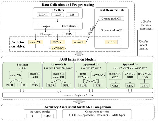
Figure 1.
The workflow of this study.
2.1. Study Sites and Experimental Design
The experimental site was in Xinxiang County, Xinxiang City, Henan Province, China (35°8′ N, 113°45′ E), specifically, at the Xinxiang Experimental Base (as shown in Figure 2) of the Chinese Academy of Agricultural Sciences. Xinxiang County is in the northern part of Henan Province, experiencing a temperate continental climate with distinct seasons [32]. The typical annual average temperature and precipitation are 14 °C and 573.4 mm. The monthly average temperature and precipitation in 2022 and 2023 are as shown in Figure A1. The overall climatic pattern is characterized by hot and rainy summers and cold and dry winters. The typical growth season for soybeans in the area is from June to October. In 2022, the region experienced relatively dry conditions before sowing, followed by several heavy rainfall events in July. To ensure normal crop growth, field management measures such as irrigation and drainage were implemented. The dominant soil type is Calcaric Fluvisols (http://www.soilinfo.cn/map/, accessed on 20 April 2025) and the topsoil texture class is loam [33]. Specifically in our study area, the field capacity of the soil is 35% in terms of volumetric water content [33].
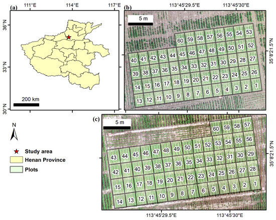
Figure 2.
Experimental design: (a) location of the study area, (b) plots for the 2022 experiment, and (c) plots in 2023. The numbers in (b,c) are the plot identification numbers.
A total of 60 plots were established for the experiment, each containing a different soybean variety, and each with an area of approximately 5.60 m2 (2.0 m × 2.8 m). Row spacing was 0.5 m, and plant spacing was 0.1 m. Experimental data were collected over two growing seasons, 2022 and 2023, with seeds sown on 20 June 2022, and 18 June 2023, respectively.
2.2. Data Collection and Preprocessing
2.2.1. Field-Measured Data
In 2022 and 2023, a total of 10 destructive sampling events were performed (Table 1). Each year, two vegetative growth stages (V4–V5 and V7–V8, corresponding to BBCH codes 14–15 and 17–18 [34]) and three reproductive growth stages (R1–R2, R3, and R4, corresponding to BBCH codes 61–65, 71, and 75, respectively [34]) were covered. At each sampling event, three consecutive soybean plants were selected from each plot. Before sampling, the CH of the three soybean plants was measured using a 5 m tape measure. In the laboratory, the underground parts of each plant were separated. The stems, leaves, and pods were weighed separately using an electronic balance at 0.1 g accuracy. After weighing, the samples were put in an oven, first at 105 °C for 2 h for inactivation, and then for drying at 85 °C until the weight stabilized. Subsequently, the dry weights of the three selected plants were measured and averaged to represent the average dry weight (DW) in that plot. Finally, dividing the average DW by its occupied area gave us the soybean AGB per unit area (g/m2). The specific calculation steps are as follows:
where DWi and DWavg correspond to the dry weight of a single soybean plant and the average dry weight within the plot (g/plant), respectively; Aplot and Nplant represent the total plot area (m2) and the total number of soybean plants in the plot, respectively; Aplant denotes the average area occupied by each individual soybean plant (m2/plant); and AGB represents the unit AGB in the plot (g/m2).

Table 1.
Soybean sampling growth stages in 2022 and 2023.
The ground-truth measurements of CH and AGB are detailed in Table A1, listing the mean, median, minimum, and maximum values for each sampling event. Following the accumulation of organic matter during crop growth, a clear increasing trend was observed in each year. In 2022, the CH increased from 0.30 m to 0.61 m, while average AGB reached 404.14 g/m2 in the R4 period. Both CH and AGB were low, mainly due to the heavy storm and hail in late July. The range was much larger in 2023, with average CH and AGB reaching 0.90 m and 633.90 g/m2, respectively.
As thermal factors are a key driving factor in plant biomass growth, we collected daily temperature information using a local meteorological station installed at the experimental area by the Chinese Academy of Agricultural Sciences. The daily maximum and minimum temperatures were obtained after soybean sowing. Due to heavy storms and equipment maintenance, some data in July were not available from the station. For these dates, missing data were supplemented with temperature records for Xinxiang County from the Tianqi website (https://lishi.tianqi.com/, accessed on 3 January 2025), which sourced its data from national meteorological stations managed by the China Meteorological Administration.
2.2.2. Remote Sensing Data from Drones
Data Collection
UAV remote sensing data were collected in both years. The specifications of the sensors and flight parameters were as listed in Table A2. In 2022, we used the DJI M300 RTK (DJI Technology Co., Ltd., Shenzhen, China), a professional-grade quadcopter UAV, for data collection. The UAV was equipped with a Micasense RedEdge-MX sensor (AgEagle Aerial Systems Inc., Wichita, KS, USA) and, simultaneously, a DJI Zenmuse L1 LiDAR sensor (DJI Technology Co., Ltd., Shenzhen, China). The Micasense RedEdge-MX sensor captured MS imagery with five wavelength bands: Blue (B, center wavelength 475 nm, bandwidth 20 nm), Green (G, center wavelength 560 nm, bandwidth 20 nm), Red (R, center wavelength 668 nm, bandwidth 10 nm), Red Edge (RE, center wavelength 717 nm, bandwidth 10 nm), and Near-Infrared (NIR, center wavelength 840 nm, bandwidth 40 nm). The DJI Zenmuse L1 LiDAR sensor was used to collect a LiDAR point cloud and RGB images. All data were collected at a flight altitude (FA) of 30 m. In 2023, the FA was adjusted to 20 m to enhance the SR. LiDAR and MS data were collected in the same manner as in 2022, but the RGB images were captured using a hexacopter DJI M600 Pro (DJI Technology Co., Ltd., Shenzhen, China) equipped with a Sony a7 II digital camera (Sony Corporation, Tokyo, Japan) to ensure high SR.
To assist with the geo-registration of the UAV data, 0.5 m × 0.5 m square plates with sharp angles were placed around the soybean plots to provide ground control points (GCPs). The accurate geographical location information (latitude, longitude, and altitude) associated with each GCP was measured using a real-time kinematic (RTK) differential global positioning system (GPS). The spatial displacement error was within a centimeter.
Data Pre-Processing
The LiDAR data were pre-processed using the DJI Terra software (version 3.5.5, DJI Technology Co., Shenzhen, China), and exported in LAS format under the WGS84/UTM Zone 49N coordinate system. These colored point clouds were then imported into ArcMap (version 10.8, Esri, Redlands, CA, USA) for further processing. To provide data for CH calculation, the point cloud was classified to identify ground points using the Conservative Filtering method provided by the Classify Las Ground (3D Analysis) tool. This method is best suited for flat terrain, such as that found in this study, effectively minimizing the misclassification between ground points and low vegetation. The parameter “Digital Elevation Model (DEM) resolution” was set to 0.3 m to accelerate the classification process. To provide data for VI calculation, the point cloud was converted to RGB images using the LAS Dataset to Raster tool [35]. The average RGB values of all points within each pixel were calculated to represent the RGB of each pixel. The pixel size was set to 0.017 m.
For the RGB data, point-cloud construction and image stitching were performed using the Agisoft Metashape software (version 2.0.2, Agisoft LLC, Saint Petersburg, Russia). The workflow began with the alignment of the photos using Structure-from-Motion (SfM) algorithms [36]; this was followed by an optimization step to minimize reprojection errors and generate sparse point clouds. The coordinates of the GCPs were manually entered using the software to enhance the spatial accuracy of the outputs. A dense point cloud was then constructed to build the orthomosaics, which provided the data for VI calculation. The point cloud was also used for CH calculation, following the same procedure as described in the paragraph above discussing LiDAR data processing.
The MS point cloud and orthomosaics were generated following a workflow similar to that of the RGB data, with two exceptions. The first exception is that a reflectance calibration step was integrated to ensure spectral consistency across acquisition dates. To facilitate the calibration, a gray panel with known reflectance in the five bands was placed on the ground; the MS photos of this panel were captured following the Micasense guidelines (https://support.micasense.com/hc/en-us/articles/1500001975662-How-to-use-the-Calibrated-Reflectance-Panel-CRP, accessed on 3 January 2025). The second exception is that GCPs were not used during the orthomosaic generation, but were utilized in a georeferencing process afterwards.
The resolutions for all the UAV data are shown in Table 2. This table lists the point spacing and image SR of the LiDAR, RGB, and MS data across different acquisition dates. The SR of LiDAR was fixed at 0.017 m, while RGB and MS data varied slightly due to differences in sensor settings and flight parameters. Due to an error with the flight path design on 23 July 2022, MS images for plots 1 through 13 were lost (see Figure 2b). The LiDAR data on 15 July 2023 was missing due to a sensor malfunction. To ensure a fair comparison of different data types (i.e., LiDAR, RGB, and MS), these 73 samples (i.e., plots 1–13 on 23 July 2022 and all 60 plots on 15 July 2023) were excluded from further analysis. As a result, a total of 527 samples were obtained for each data source.
Table 2.
Basic information associated with the UAV data.
2.2.3. Dataset Configuration
Data collected in 2022 and 2023 formed the dataset in this study. For each data source (LiDAR, RGB, and MS), there were 527 samples, each representing the data collected for one plot at one sampling time. The dataset was divided into training and testing sets with a 7:3 ratio, with around 367 in the training set and the remaining 160 in the testing set. The same splits were used for all the AGB estimation models to ensure that the model comparison was not affected due to sample difference.
To ensure the stability and reliability of the results, the training/testing split was repeated 20 times with 20 fixed random seeds. The average accuracy of the 20 repetitions was used to represent the overall model performance, while the standard deviation was calculated in order to determine model robustness.
2.3. CH Estimation
CH is a key factor in estimating crop biomass. We employed two methods and the previously described three data sources to calculate CH, aiming to compare the accuracy and applicability of these methods and sources, thus providing a scientific basis for crop growth monitoring and biomass estimation.
2.3.1. Per-Pixel CH
The classified point-cloud data were used to generate the Digital Surface Model (DSM) and Digital Terrain Model (DTM). First, the point cloud was rasterized to DSM, the pixel value of which was the elevation of the highest point within the pixel. Next, ground points were used to generate the DTM, which reflects the elevation of the ground. Using the Raster Calculator in ArcGIS, the DSM was subtracted from the DTM to produce the Canopy Height Model (CHM) [37]. In the CHM, each pixel value represents the crop height (Hi) of that pixel.
2.3.2. Per-Plot CH
The plot-level mean CH was determined by calculating the differences between specific percentiles of the point cloud in each plot.
where Z1 and Z0 are distinct percentiles of the elevation within the plot point cloud.
Different combinations of Z1 (99–80%, with 1% steps) and Z0 (5–0%, with 1% steps) were considered. For each data source (i.e., LiDAR, RGB, and MS), CHs calculated from these 120 combinations were compared to the field-measured CHs. The combination with the highest accuracy was selected as the optimal metric and used for the subsequent CH calculations.
2.4. Soybean AGB Estimation
This study considered three approaches to the use of CH in AGB estimation. The first approach (Approach 1) inputs the mean VIs and CH as separate variables into the PLSR and RFR models to estimate AGB. The second approach (Approach 2) integrates VIs and CH to construct composite indices, which are then input into the PLSR and RFR models for AGB estimation. The third approach (Approach 3) inputs GS information, CH, and the composite indices into the CBA model to estimate AGB. To better understand the contribution of CH in AGB estimation, these three approaches were compared to the baseline model which does not use CH input.
2.4.1. Baseline Model (No CH): AGB Estimation with VIs
Spectral Indices
A total of 16 VIs were extracted from the LiDAR and RGB images respectively, and 20 VIs were extracted from the MS images. The purpose of extracting multiple VIs is to fully utilize the rich spectral information, thus capturing different aspects of crop growth and improving the accuracy of biomass estimation. These indices are commonly used in soybean AGB studies [38,39]. Their integration effectively reduces noise and interference, yielding more comprehensive and stable predictive results. Table A3 and Table A4 provide the definitions and reference values of these VIs, where R, G, B, RE, and NIR represent reflectance in the red, green, blue, red-edge, and near-infrared bands, respectively. The zonal averages of the indices were calculated to represent the mean VIs of each plot.
Machine Learning Models
To avoid issues in estimation models (e.g., high dimensionality, noise interference, and multicollinearity among variables), this study adopted two machine learning methods that can effectively handle high-dimensional data and multicollinearity while capturing complex nonlinear relationships. They are Partial Least Squares Regression (PLSR) and Random Forest Regressor (RFR). Grid search was adopted in parameter optimization to improve model performance. Using the training dataset, the parameters for each machine learning model were optimized through grid search with 10-fold cross-validation. The trained models with optimal parameters were then applied to the testing dataset to assess their performance.
PLSR [40] combines the benefits of Principal Component Analysis (PCA) and Multiple Linear Regression by projecting data into a new, low-dimensional space for regression analysis. By extracting latent variables, PLSR effectively resolves multicollinearity issues, yielding stable and accurate predictions. During the hyperparameter tuning, the number of latent variables was set to range from 1 to the number of features. The optimal number of latent variables was found using 10-fold cross-validation. For each data type (LiDAR, RGB, or MS), all the mean VIs were included as predictor variables in the model.
RFR [41] involves multiple decision trees, with each tree independently learning from the sample data and generating predictions. By averaging the predictions from all decision trees, the random forest effectively captures complex patterns and nonlinear relationships in the data, improving prediction accuracy and reducing the risk of overfitting. As a result, random forests demonstrate high accuracy in predicting crop AGB. To ensure the reproducibility of model training, four parameters were optimized with 10-fold cross-validation. The parameter grid includes the following values: number of trees (100, 200, and 300), maximum depth (unlimited, 10, 20, and 30), minimum number of samples for splitting nodes (2, 5, and 10), and minimum number of samples in leaf nodes (1, 2, and 4). For each data type (LiDAR, RGB, or MS), all the mean VIs were included as predictor variables in the model.
Hierarchical Regression Considering Growth Stages
The relationship between VIs and AGB changes gradually as crop plants grow. Therefore, we adopted a hierarchical regression approach called CBA [30], originally proposed for wheat, to improve soybean AGB estimation. CBA assumes a linear correlation between VIs and AGB (Equation (6)), with the slope k and intercept b fitted to phenological indicators (Equation (7)) such as day of year, the Zadok’s scale, and growing-degree days (GDD).
This hierarchical structure allows AGB estimation to adapt to crop development by dynamically adjusting regression parameters based on thermal time. In this study, we used GDD as the phenological indicator, which more accurately captures temperature’s influence on biomass accumulation throughout the plant growth stages [30]. Combining Equations (6) and (7), the complete form of the model is as follows:
where i denotes the i-th sample plot at a given phenological stage, and k(GDD) and b(GDD) were modeled as quadratic polynomial functions.
GDD was calculated using Equation (11):
where DAS denotes the days after sowing, Tmax and Tmin refer to the maximum and minimum temperatures for each DAS, and Tbase is the base temperature of the crop. In this study, the base temperature was set to 10 °C [42]. Figure A2 illustrates the daily maximum/minimum temperatures and the cumulative GDD trends during the soybean growing seasons of 2022 and 2023, with sowing and sampling dates also indicated.
Each mean VI was used to construct a separate CBA model, because different VIs exhibit distinct sensitivities and temporal response patterns relative to crop growth. The most accurate one was selected to represent the baseline CBA method for comparison with other approaches.
2.4.2. Approach 1: CH as an Additional Predictor in Machine Learning Models
In Approach 1, PLSR and RFR were used to construct the AGB estimation models. As distinct from the baseline machine learning models (Section Machine Learning Models), mean CH was input as an additional predictor variable. The models were constructed and validated following the same data processing workflow. Grid search and 10-fold cross-validation were used to optimize the same hyperparameters described in the context of Section Machine Learning Models. The trained optimal models were then applied to the test dataset to evaluate their predictive performance. After repeating this 20 times, the average accuracy and its standard deviation were computed to represent the model correctness and robustness.
2.4.3. Approach 2: CH Fused with VIs to Generate CVMVI Variables
Integrating CH with VI to form a new index is an effective approach. We adopted a multiplicative approach for the fusion, which aligns with the physical interpretation of AGB: biomass is the product of volume and density. CH multiplied by canopy area approximates the volume, while VIs characterize the mass density. Thus, the product of CH and VI has a theoretical ground in estimating AGB. Previous studies have explored both pixel-wise multiplication [28] and average-based multiplication [43]. In this study, we evaluated and compared the performance of these two fusion strategies.
Per-Pixel Fusion
Following Maimaitijiang, Sagan [28], we calculated CVMVI based on the pixel-level CHM. The CHM images from the corresponding data sources were multiplied across the VI images. The cumulative sums of the resulting values for the entire plot were then calculated to form CVMVIs.
where i represents the i-th soybean pixel, Apixel represents the pixel area, Hi represents the crop height of the i-th pixel, VIi represents the vegetation index value of the i-th pixel, and n represents the total number of pixels in the plot. We tested different values of m and found that m = 1 provided the best results for AGB estimation. Therefore, we used m = 1 throughout the experiment.
The CVMVIs were calculated for each VI, resulting in 16 CVMVIs for the LiDAR and RGB data and 20 CVMVIs for the MS data. The CVMVIs from each data source were then used as predictor variables in both the PLSR and RFR models to predict AGB.
Per-Plot Fusion
Compared to the study area in Maimaitijiang, Sagan [27], the plots in this study were smaller and featured higher planting density, making it nearly impossible to identify the exact area for the sampled plants. To address this issue, we developed an alternative model, based on mean CH and VI values, referred to as mean-based CVMVI (mCVMVI).
where Aplot represents the plot area, CHmean represents the average plant height of soybeans across the entire plot, and VImean denotes the mean VI for each plot. In this formula, m is similarly set to 1.
Similarly to the process used for CVMVIs, the mCVMVI was calculated for each VI, resulting in 16 CVMVIs for the LiDAR and RGB data and 20 CVMVIs for the MS data. For each data source, the mCVMVIs were then used as predictor variables in both the PLSR and RFR models to predict AGB.
2.4.4. Approach 3: Hierarchical Regression Considering Growth Stages
This approach considers both CH and GS information. Similarly to the baseline hierarchical regression model, we adopted the CBA method. To incorporate CH information, the VI in the original CBA model was replaced with CH-related variables. Three different models were constructed.
where k(GDD) and b(GDD) were modeled using quadratic polynomial functions.
Using Equation (6), the CBA–CH models were built for each data type. For CVMVI, each CVMVI was used to construct a separate CBA–CVMVI model. For mCVMVI, each mCVMVI was used to construct a separate CBA–mCVMVI model. Among all these models, the most accurate one was then selected to represent Approach 3 for use in comparison with other approaches.
To evaluate the contribution of GDD to soybean AGB estimation, we designed an ablation experiment in which all GDD values were replaced with the global mean. Comparing the AGB estimation results using these average GDD values with the results obtained using actual GDD information allowed a direct assessment of the improvements in AGB estimation contributed by GDD.
2.5. Accuracy Assessment
To evaluate the accuracy of the biomass estimation models, we selected the coefficient of determination (R2) [44], root mean square error (RMSE) [45], mean absolute error (MAE) [46], and mean relative error (MRE) [47] as the evaluation metrics. R2 represents the proportion of variance in the dependent variable explained by the independent variables. A higher R2 value indicates stronger explanatory power and better model performance.
RMSE, MAE, and MRE all measure the deviation between the predicted and actual values. RMSE reflects the average level of prediction error, representing the standard deviation of the residuals. MAE represents the average magnitude of the absolute differences between predicted and observed values. Compared to RMSE, MAE is less sensitive to large errors. MRE represents the average relative difference between predicted and observed values, expressed as a percentage. Unlike MAE, MRE takes the scale of the actual values into account, making it particularly useful for understanding the error in relation to the magnitude of the observations. Lower RMSE, MAE, and MRE indicate better model performance.
where and are the ground truth and estimated values of the target variable (AGB or CH, in this study) for the i-th plot, is the average value of , and n is the number of samples.
With accuracy metrics from the 20 runs representing the performance of each method, we first performed a one-way Analysis of Variance (ANOVA) to confirm the significance of differences among methods. Subsequently, Tukey’s HSD (Honest Significant Difference) test was conducted for multiple-group pairwise comparisons. Note that the comparison is among different methods using the same type of UAV date. Statistically significantly different methods are denoted with distinct letters [48].
3. Results
3.1. CH Estimation Results
Based on Equation (5), we obtained the predicted CH values that best fit the measured CH from various data sources. For LiDAR point-cloud data, using the difference between the 94th percentile and the zero percentile as the prediction parameter yielded the best fit, with accuracy of R2 = 0.85 and an RMSE = 0.09 m, as shown in Figure 3a. For RGB data, optimal prediction performance was achieved using the difference between the 88th percentile and the zero percentile, resulting in a slightly diminished accuracy of R2 = 0.84 and RMSE = 0.09 m, as shown in Figure 3b. For MS data, the difference between the 85th percentile and the zero percentile produced the best results, with R2 = 0.65 and RMSE = 0.13 m, as shown in Figure 3c.
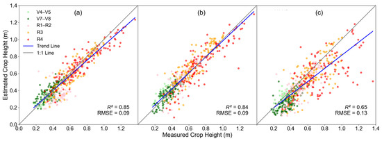
Figure 3.
Comparison of estimated and measured CHmean from different data sources: (a) LiDAR, (b) RGB, and (c) MS.
In summary, both the LiDAR and the RGB data exhibited higher accuracy in CH prediction, while the performance of MS data was lower. Meanwhile, a slight underestimation was observed for larger CH values when using LiDAR or RGB as the data source. The underestimation was more pronounced using the MS data.
3.2. Comparison of AGB Estimation Models
The AGB estimation accuracy showed a generally increasing trend from the baseline models to Approach 3 (Table 3, Figure 4). In Figure 4, the letters indicate the results of Tukey’s HSD test. Among the five types of methods (i.e., baseline multi-variate machine learning, baseline CBA, Approach 1, Approach 2, and Approach 3), those annotated with different letters are significantly different at the 0.05 significance level. The baseline multi-variate machine learning method exhibited the lowest accuracy, which was statistically significant regardless of the data source. This highlighted the importance of CH input in soybean AGB estimation. Approach 2 had higher accuracy than Approach 1, indicating that CH and VI fusion was better than simple combinations. However, statistically significant differences between Approach 2 and Approach 1 were only observed with the MAE metric for LiDAR and RGB, as well as the MRE metric for RGB. The accuracy improvement from Approach 1 is not guaranteed, but the fusion method needs careful selection. The best Approach 2 model for LiDAR and RGB were the PLSR model with mCVMVIs as input variables, while for MS, it was the RFR model with CVMVIs as inputs. Adding GDD into consideration, Approach 3 achieved the highest accuracy among all approaches.
Table 3.
Performance metrics averages (20 runs), by method and sensor.
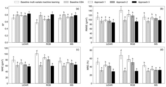
Figure 4.
Comparison of AGB estimation accuracy using different CH-use approaches: (a) R2; (b) RMSE; (c) MAE; and (d) MRE. Note: the letters above each bar indicate the results of the Tukey’s HSD. Bars marked by different letters have statistically significantly different accuracy.
Two exceptions to the trend were observed. First, the baseline CBA method using only VIs outperformed Approach 1 and Approach 2. For all three data types, the baseline CBA method achieved high accuracy (R2 ≥ 0.79, RMSE ≤ 97.88 g/m2, MAE ≤ 61.43 g/m2, MRE ≤ 31.29%). This suggests that the GS information may contribute more to the AGB estimation than CH to AGB estimation. Nevertheless, adding GDD led to increased accuracy for both the LiDAR (R2 = 0.83, RMSE = 87.52 g/m2, MAE = 57.29 g/m2, MRE = 28.59%) and the RGB data (R2 = 0.81, RMSE = 91.86 g/m2, MAE = 58.93 g/m2, MRE = 29.55%). With LiDAR as the data source, the R2 of Approach 3 was statistically significantly higher than all other methods. Second, using the MS data, the baseline CBA model achieved slightly higher accuracy (R2 = 0.81, RMSE = 92.94 g/m2, MAE = 59.34 g/m2, MRE = 30.08%) than Approach 3 (R2 = 0.79, RMSE = 97.99 g/m2, MAE = 63.04 g/m2, MRE = 31.41%), although this was not statistically significant. The R2 and RMSE separate the MS models into two groups, with GDD-involved models (i.e., baseline CBA model and Approach 3) having higher accuracy than those without GS information (i.e., baseline machine learning models, Approach 1, and Approach 2).
3.2.1. Baseline Model (No CH): Estimating Soybean AGB Using VIs
The baseline models showcase the performance of soybean AGB estimation without CH in the input. The most accurate results among the 20 runs are illustrated in Figure 5 for each type of model. With the PLSR models, the highest accuracy was achieved using the MS data (R2 = 0.78, RMSE = 100.29 g/m2, MAE = 67.74 g/m2, MRE = 33.51%, Figure 5c), followed by LiDAR (R2 = 0.77, RMSE = 92.46 g/m2, MAE = 70.06 g/m2, MRE = 44.77%, Figure 5a) and RGB (R2 = 0.64, RMSE = 127.65 g/m2, MAE = 93.18 g/m2, MRE = 56.01%, Figure 5b). With the RFR models, the same trend was found, with MS demonstrating the best performance (R2 = 0.76, RMSE = 104.89 g/m2, MAE = 68.00 g/m2, MRE = 32.47%, Figure 5f), followed by LiDAR (R2 = 0.73, RMSE = 117.81 g/m2, MAE = 83.56 g/m2, MRE = 50.05%, Figure 5d) and RGB (R2 = 0.55, RMSE = 146.06 g/m2, MAE = 98.42 g/m2, MRE = 56.75%, Figure 5e). These confirmed that the RE and NIR bands in the MS data provide valuable spectral information that complements the visible bands in soybean AGB estimation.
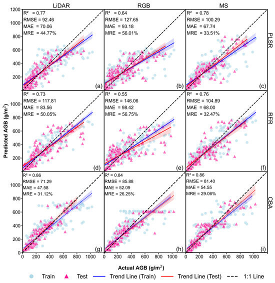
Figure 5.
Soybean AGB estimation results of the baseline (no CH) models (best of the 20 runs): (a) PLSR–LiDAR; (b) PLSR–RGB; (c) PLSR–MS; (d) RFR–LiDAR; (e) RFR–RGB; (f) RFR–MS; (g) CBA–LiDAR; (h) CBA–RGB; and (i) CBA–MS.
In contrast, with the CBA models which included GDD as additional input, all three data types performed similarly (R2 = 0.84–0.86, RMSE = 71.29–85.88 g/m2, MAE = 47.58–54.55 g/m2, MRE = 26.25–31.12%, Figure 5g–i). Detailed accuracy information for each CBA-VI is listed in Appendix B (Table A5, Table A6 and Table A7). For the LiDAR data, GLI2 was the best-performing VI. For RGB, the best-performing index was RGBVI. For MS, the best-performing index was CI_G. Compared to the PLSR and RFR models, the CBA models significantly improved AGB estimation, although the number of predictor variables was much smaller. This confirms that GDD improves AGB prediction even without CH inclusion.
3.2.2. Approach 1: CH as an Additional Predictor in Machine Learning Models
For Approach 1, we introduced CH as an additional input variable alongside VIs to enhance soybean AGB prediction. The results from different data sources and machine learning models are presented in Figure 6. For PLSR models, the best performance was achieved using LiDAR data, with an accuracy of R2 = 0.82, RMSE = 87.98 g/m2, MAE = 59.31 g/m2, and MRE = 39.42%, as shown in Figure 6a. The PLSR–RGB model exhibited lower accuracy, with R2 = 0.73, RMSE = 109.52 g/m2, MAE = 81.05 g/m2, and MRE = 64.19%, as shown in Figure 6b, while the PLSR–MS model performed better, achieving R2 = 0.81, RMSE = 88.44 g/m2, MAE = 65.58 g/m2, and MRE = 41.79%, as shown in Figure 6c. For RFR models, the highest accuracy was observed in RFR–LiDAR, with R2 = 0.81, RMSE = 86.92 g/m2, MAE = 59.31 g/m2, and MRE = 47.40%, as shown in Figure 6d. The RFR–MS model performed comparably well, with R2 = 0.79, RMSE = 90.81 g/m2, MAE = 61.30 g/m2, and MRE = 32.53%, as shown in Figure 6f, whereas the RFR–RGB model had the lowest accuracy, with R2 = 0.73, RMSE = 112.59 g/m2, MAE = 78.17 g/m2, and MRE = 42.06%, as shown in Figure 6e.
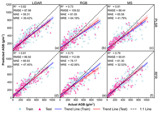
Figure 6.
Soybean AGB estimation results for the Approach 1 models (best of the 20 runs): (a) PLSR–LiDAR; (b) PLSR–RGB; (c) PLSR–MS; (d) RFR–LiDAR; (e) RFR–RGB; and (f) RFR–MS.
In summary, the addition of CH significantly improved the model’s fit for both training and testing datasets, with scatter points aligning more closely to the 1:1 line and a notable reduction in RMSE. This indicates that CH effectively compensates for the limitations of spectral information, enhancing AGB estimation accuracy, especially when combined with LiDAR data.
3.2.3. Approach 2: CH Fused with VIs to Generate CVMVI Variables
The results of Figure 7 and Figure 8 indicate that, compared to the baseline model without CH (Figure 5a–f), incorporating CVMVI and mCVMVI significantly improved AGB estimation accuracy. Using LiDAR or RGB data, mCVMVI demonstrated overall better performance relative to CVMVI, while for MS it was the other way round. Among all Approach 2 models, the best performance was achieved with PLSR–LiDAR (mCVMVI), reaching R2 = 0.83, RMSE = 85.49 g/m2, MAE = 60.28 g/m2, and MRE = 40.72% (Figure 8a). This was followed by RFR–LiDAR (mCVMVI), which also performed well, achieving R2 = 0.80, RMSE = 88.83 g/m2, MAE = 68.97 g/m2, and MRE = 52.18% (Figure 8d). In comparison, the best result under CVMVI was obtained with RFR–MS, yielding R2 = 0.79, RMSE = 95.02 g/m2, MAE = 61.81 g/m2, and MRE = 32.24% (Figure 7f). Nonetheless, overall, mCVMVI demonstrated lower MRE and a more stable fitting performance.
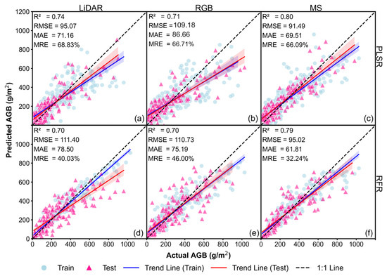
Figure 7.
Soybean AGB estimation results for the Approach 2 models with CVMVIs (best of the 20 runs): (a) PLSR–LiDAR; (b) PLSR–RGB; (c) PLSR–MS; (d) RFR–LiDAR; (e) RFR–RGB; and (f) RFR–MS.
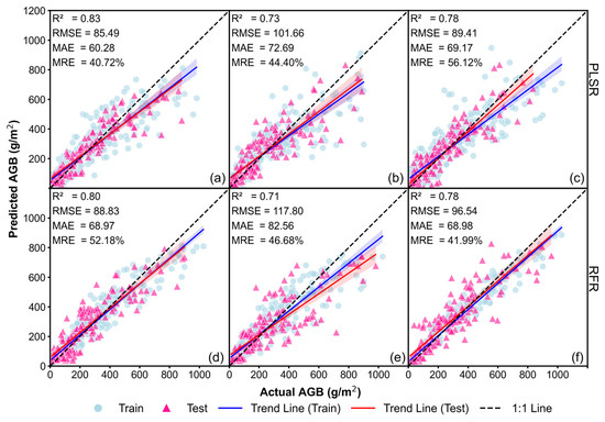
Figure 8.
Soybean AGB estimation results for the Approach 2 models with mCVMVIs (best of the 20 runs): (a) PLSR–LiDAR; (b) PLSR–RGB; (c) PL SR–MS; (d) RFR–LiDAR; (e) RFR–RGB; and (f) RFR–MS.
3.2.4. Approach 3: Hierarchical Regression Considering Growth Stages
For Approach 3, we applied the CBA model to optimize soybean AGB estimation accuracy by incorporating the GDD and CH information. For all three data sources, we calculated the estimation results for the mean CH and for both composite variables (see Table A5, Table A6 and Table A7). From each category, the highest-performing results are illustrated in Figure 9. For LiDAR data, the best result was obtained with mCVMVIGLI2 (R2 = 0.86, RMSE = 81.64 g/m2, MAE = 54.88 g/m2, and MRE = 25.67%, Figure 9g), followed by using CH and no VI (R2 = 0.86, RMSE = 80.12 g/m2, MAE = 53.89 g/m2, and MRE = 28.11%, Figure 9a), and then CVMVIGLI2 (R2 = 0.83, RMSE = 89.35 g/m2, MAE = 56.80 g/m2, and MRE = 28.05%, Figure 9d). For RGB data, the same trend was observed, with mCVMVIGN achieving the highest accuracy (R2 = 0.86, RMSE = 81.16 g/m2, MAE = 52.68 g/m2, and MRE = 28.29%, Figure 9h). For MS data, in contrast, CVMVIARI_2 yielded the best performance (R2 = 0.84, RMSE = 86.67 g/m2, MAE = 55.39 g/m2, and MRE = 27.16%, Figure 9f), while MS–CH had the lowest prediction accuracy (R2 = 0.83, RMSE = 89.35 g/m2, MAE = 57.88 g/m2, and MRE = 29.50%, Figure 9c).
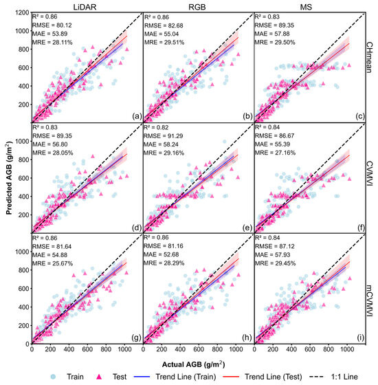
Figure 9.
Soybean AGB estimation results for the Approach 3 models with mCVMVIs (best of the 20 runs): (a) LiDAR–mean CH; (b) RGB–mean CH; (c) MS–mean CH; (d) LiDAR–CVMVIGLI2; (e) RGB–CVMVIEXB; (f) MS–CVMVIARI_2; (g) LiDAR–mCVMVIGLI2; (h) RGB–mCVMVIGN; (i) MS–mCVMVICI_G.
Among all the Approach 3 models, LiDAR–mCVMVIGLI2 achieved the highest prediction accuracy. Compared to the baseline model, Approach 1, and Approach 2, the inclusion of GDD and CH information significantly improved AGB estimation accuracy, as evidenced by higher R2 values and lower RMSE, MAE, and MRE across all sensor types.
Furthermore, the contribution of GDD to soybean AGB estimation was confirmed through an ablation experiment in which the original GDD values were replaced by the average GDD. Without the GDD information, the AGB estimation accuracy significantly decreased (Table 3, compared to Table 4). Using the best-performing composite variable (i.e., mCVMVI) as an example, the incorporation of GDD increased the R2 for LiDAR from 0.55 to 0.83 (an increase of 50.9%), and decreased RMSE from 142.51 g/m2 to 87.52 g/m2 (a reduction of 38.6%). For RGB, R2 improved from 0.48 to 0.81 (an increase of 68.8%), and RMSE dropped from 153.41 g/m2 to 58.93 g/m2 (a reduction of 61.6%). For MS data, R2 increased from 0.51 to 0.79 (a gain of 54.9%), and RMSE decreased from 148.27 g/m2 to 61.39 g/m2 (a reduction of 58.6%), while MAE decreased by 43.6% (from 111.71 g/m2 to 63.04 g/m2).
Table 4.
Ablation experiment for GDD: AGB estimation performance by fixing GDD at the average level (20 runs).
4. Discussion
4.1. CH Estimation Accuracy Relative to Different Data Types
LiDAR and RGB outperform MS in CH prediction accuracy (Figure 3). Similar trends have also been found in previous studies. The LiDAR dataset directly measures three-dimensional spatial information [37,49]. Therefore, the LiDAR point cloud well represents crop height structure, showing excellent performance, especially in low plant-height regions (e.g., V4–V5 stages) [29]. The high resolution and rich texture information of the RGB data enable accurate capture of the vegetation’s morphological characteristics, particularly in medium to high plant-height ranges [28]. In contrast, the lower accuracy of MS data in CH prediction may be due to its lower SR and the weaker correlations between its spectral features and plant height [50].
To understand the rationale behind the CH accuracy difference, we checked the point clouds of individual plots (Figure 10). Firstly, the most obvious difference is that LiDAR data and RGB data have much denser point clouds than those associated with MS data. This is because the MS images had much lower SR values (Table 2). As a result, the LiDAR and RGB point clouds contain more structural details, compared to the MS data. Secondly, the visibility of the ground below the canopy is different among the three data types. LiDAR has better canopy penetration, with many returns from the ground despite the dense canopy [37]. The RGB point cloud, though, contains little information below the crop canopy, but was able to determine the ground elevation proximate to the crops, possibly thanks to its very high SR (finer than 2 mm). The MS results are associated with severe underestimation, mainly because no ground elevation was collected for many of the plots (e.g., Figure 10f). Efforts aiming to refine the MS image SR by using enhanced sensors or adjusting the flight design may alleviate the problem. It is also possible to combine LiDAR- or RGB-based CH with MS-based VIs, as long as the data are accurately geo-registered.
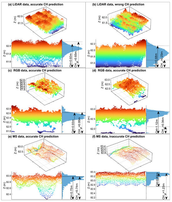
Figure 10.
Illustration of CH prediction errors, along with the corresponding point clouds. Note: The color corresponds to height (Z), with red color indicating higher points and blue color indicating lower points.
Further analysis of prediction errors reveals that some seemingly inaccurate CH estimations may be due to uncertainties in the ground truth data (Figure 10b,d). This is mainly attributed to the high heterogeneity of soybean growth within plots. When measuring actual plant height, we randomly selected three consecutive plants rather than deliberately choosing representative ones. An adjustment of field sampling strategy may be required in future studies.
Although CH was accurately estimated from the LiDAR data in general, the larger CH values tend to be underestimated (Figure 3). This may be attributed to the changes of canopy structure in different growth stages. As the growth progresses, the plant height increases alongside the development of different organs. Consequently, the point-cloud distribution (Figure 10) evolves, which causes the most representative Z1 and Z0 for the plot-average CH to change. Additionally, the different climatic conditions in 2022 and 2023 (Figure A1) could also have contributed to the variance of soybean CHs in this study. Therefore, further investigation into the reason for the underestimation is required. Meanwhile, future studies may consider optimizing the selection of Z1 and Z0 separately for different growth stages.
4.2. CH Contribution to AGB Estimation
The results of this study indicate that composite variables (Approach 2) outperform simple combination of the variables (Approach 1) in AGB estimation, which may be closely related to the complex three-dimensional canopy structure characteristics of AGB. The advantage of Approach 1 over baseline machine learning models is also supported by previous AGB estimation studies [27,29]. However, the vertical canopy structure of soybeans may not be fully exploited, as it only takes up a small portion of the input (e.g., one CH vs. 16 VIs for LiDAR). This study demonstrated that the estimation accuracy of composite variables is superior to that of simple combinations, highlighting the advantages of composite variables in AGB estimation. Additionally, incorporating GDD into the composite variables further improved the accuracy of soybean AGB estimation, which is consistent with findings from studies on maize biomass estimation [38].
Notably, as observed in Figure 4, in the LiDAR and RGB data sources, the estimation accuracy of the CBA model was lower when only VI and GDD information were used as inputs (baseline CBA) compared to when composite variables and GDD information were jointly included (Approach 3). However, in the MS data source, the opposite trend was observed. This phenomenon may be attributed to the lower accuracy of plant-height estimation in MS data, which in turn affects the final AGB estimation performance. Since composite variables are more dependent on crop structural information, the inaccurate CH estimates in MS data may reduce the effectiveness of composite variables. Meanwhile, the results also confirm the advantage of MS data in providing useful spectral information, as the baseline CBA model with MS input was only slightly below the best model (Approach 3 CBA–LiDAR–mCVMVI) in this study.
Future work on crop AGB estimation should try to provide accurate CH, VI, and GDD inputs into the Approach 3 model. To make full use of the rich spectral information and the valuable CH information, it would be worthwhile to investigate the fusion of MS-based VIs and LiDAR-based CH. One potential holdback is the spatial registration of the two data sources. With such high SR, a small displacement may result in large deviations. One alternative is to employ MS cameras with higher SR, e.g., MicaSence RedEdge-P with a panchromatic image, for significant resolution refinement.
4.3. CH–VI Fusion: Comparison of CVMVI and mCVMVI
In previous studies, CVMVI was used to estimate biomass by accumulating the CH and VIs values of all pixels within each biomass sampling point [5,28]. The mCVMVI method used in this study adopted a plot-average-based fusion of the CH and VIs, rather than considering individual pixels. This approach, compared to pixel-based accumulation, overlooks local heterogeneity. However, due to the small plot size, small plant spacing, and high planting density in this study, it was not possible to identify the exact pixels associated with the sampled plants. Compared to CVMVI, mCVMVI better reflects the overall vegetation condition within the plot under high planting density, reduces the interference of local heterogeneity on the results, and provides a smoother and more stable representation.
The average-based mCVMVI exhibited higher R2 and lower RMSE, relative to CVMVI, in AGB estimation. This indicates that the average-based CVMVI, compared to the cumulative-based AGB estimation, can more effectively capture the overall vegetation characteristics within the plot, providing more accurate and stable AGB prediction results.
4.4. Hierarchical Regression with GDD
The results of this study highlight the critical role of GS information (GDD in this study) in improving AGB estimation. By incorporating GDD, the model was able to better capture the temporal variations in biomass accumulation which are associated with phenological development. Unlike conventional regression approaches which check the direct correlation between AGB and the input variable, the hierarchical regression model notices that the relationship between AGB and the input variable gradually changes as the crop plants grow [30]. As illustrated in Figure A3, the slopes show a gradually increasing trend. The hierarchical structure successfully accommodated this GS-induced variability, leading to more robust and biologically meaningful estimations. This method has been proposed for winter-wheat AGB estimation using spectral VIs as the input variable. This study successfully extended the concept to apply this method to CH and CH–VI composite variables.
As the relationship between GDD and crop growth is somewhat universal, the hierarchical regression method can possibly be generalized to other regions. Whether a universal set of coefficients can be directly transferred within studies focusing on different regions or times is a question worth exploration. One potential obstacle in applying the method is the availability of temperature data. We were able to collect temperature data, using a locally installed meteorological station, which closely reflected the GDDs of the samples. In cases where local observations are limited, we infer that data from a farther-away meteorological station can also be helpful. Such data may be obtained from open-access websites such as http://www.meteomanz.com/ (accessed on 30 April 2025) [37]. Moreover, global reanalysis datasets such as the land component of the fifth generation of European ReAnalysis (ERA5-Land) [51] and Modern-Era Retrospective analysis for Research and Applications version 2 (MERRA-2) [52] provide reliable high-resolution alternatives. Nevertheless, the sensitivity of the model to uncertainties in GDD needs to be evaluated.
4.5. Future Work
In addition to what has been discussed above, there are still multiple aspects of UAV-based soybean AGB estimation studies to be investigated. Here we would like to emphasize two of them.
The first is the need to further investigate the suitability of different VIs, modeling methods, and fusion strategies under varying crop growth stages and biomass levels. This would help us better understand the relationships between these factors and AGB estimation, so that we could develop more targeted and robust AGB estimation frameworks.
In addition to model design and input refinement, we would also like to call attention to the generalizability of the method. Since the 20 repetitions and the significance test demonstrated the robustness of the models, it would be interesting to determine whether a smaller training set (10–30%) would provide accurate models for a larger validation set (70–90%). We also plan to feed more data into the model to improve the training representability and check the applicability of the trained model to other years or study areas.
5. Conclusions
This study analyzed the performance of different data sources (LiDAR, RGB, and MS) and input variable combinations in estimating soybean AGB, with a focus on the role of CH. The main findings are as follows:
- LiDAR and RGB are equally effective in CH estimation, while MS data suffer underestimations due to the loss of ground-elevation information.
- The inclusion of CH as input data improved the soybean AGB estimation accuracy. Regardless of how the CH variable was used, the new models always outperform machine learning models with no CH input. However, for MS data, the accuracy increased less, possibly due to the poor CH-estimation results.
- CH–VI composite variables (Approach 2) more accurately represent the three-dimensional structural characteristics of crops than does simple combination (Approach 1), demonstrating superior AGB estimation performance. The composite variables like mCVMVI showed significant advantages in the context of data sources with high CH-estimation accuracy.
- The inclusion of GDD information allowed for a more accurate representation of crop dynamics across different growth stages. With accurate CH input, the integration of CH, VI, and GDD yields the most accurate AGB estimation. However, if the CH estimation is inaccurate, to only integrate VI and GDD could be a more robust choice. The hierarchical regression approach, by incorporating GDD as a dynamic modifier of the regression parameters, proves effective in improving AGB estimation accuracy.
- To enhance the robustness and generalizability of AGB estimation models, future studies should focus on improving the CH prediction accuracy of MS data, optimizing composite variable computation methods, and exploring their applicability across different crop types and environmental conditions.
Author Contributions
Conceptualization: D.Y. and Y.Z.; Methodology: D.Y. and Y.Z.; Validation: Y.Z.; Formal analysis: Y.Z.; Resources: Z.Z.; Data curation: Y.Z., X.Y., T.J., L.L., Y.L., Y.B., Z.T. and S.L.; Writing—original draft preparation: Y.Z.; Writing—review and editing: D.Y., X.Y. and X.J.; Project administration: Z.Z. and X.J.; Funding acquisition: F.F., D.Y. and X.J. All authors have read and agreed to the published version of the manuscript.
Funding
This research was supported by the Agricultural Biological Breeding Major Project (2022ZD0401801), Nanfan Special Project, CAAS (YBXM2401, YBXM2402, PTXM2402), Central Public-Interest Scientific Institution Basal Research Fund of the Chinese Academy of Agricultural Sciences (CAAS-CSAL-202402), National Natural Science Foundation of China (42071426, 42301427), and The Agricultural Science and Technology Innovation Program of the Chinese Academy of Agricultural Sciences.
Institutional Review Board Statement
Not applicable.
Data Availability Statement
Data are available on request.
Acknowledgments
The authors would like to thank the staff of the Xinxiang Experimental Base of the Chinese Academy of Agricultural Sciences for their help with the plot management.
Conflicts of Interest
The authors declare no conflicts of interest.
Appendix A
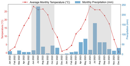
Figure A1.
Monthly temperature and precipitation for the study area in 2022 and 2023. The gray shaded area marks the soybean growth season (June to October).
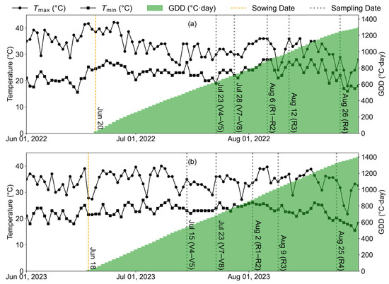
Figure A2.
Daily temperature and GDDs during the experiment: (a) 2022; (b) 2023.
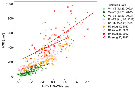
Figure A3.
Illustration of the hierarchical regression: linear correlations in different growth stages between the AGB and the input index, using the LiDAR-based mCVMVIGLI2 as an example.
Appendix B
Table A1.
Descriptive statistics of CH and AGB, from field measurements.
Table A1.
Descriptive statistics of CH and AGB, from field measurements.
| Date | CH (m) | AGB (g/m2) | ||||||
|---|---|---|---|---|---|---|---|---|
| Mean | Median | Min | Max | Mean | Median | Min | Max | |
| 23 July 2022 | 0.30 | 0.30 | 0.17 | 0.41 | 34.46 | 33.93 | 12.56 | 73.32 |
| 28 July 2022 | 0.31 | 0.30 | 0.17 | 0.48 | 52.70 | 50.91 | 15.34 | 101.87 |
| 6 August 2022 | 0.44 | 0.44 | 0.29 | 0.66 | 118.75 | 113.26 | 45.39 | 295.79 |
| 12 August 2022 | 0.53 | 0.55 | 0.31 | 0.77 | 195.06 | 200.47 | 49.45 | 363.83 |
| 26 August 2022 | 0.61 | 0.62 | 0.34 | 0.92 | 404.14 | 381.23 | 116.18 | 900.4 |
| 15 July 2023 1 | 0.27 | 0.28 | 0.18 | 0.37 | 38.01 | 37.34 | 19.74 | 60.98 |
| 23 July 2023 | 0.42 | 0.42 | 0.26 | 0.54 | 113.21 | 128.03 | 57.50 | 213.44 |
| 2 August 2023 | 0.61 | 0.64 | 0.23 | 0.77 | 276.97 | 273.98 | 111.53 | 475.54 |
| 9 August 2023 | 0.77 | 0.81 | 0.32 | 1.00 | 422.41 | 422.41 | 195.44 | 881.26 |
| 25 August 2023 | 0.90 | 0.92 | 0.44 | 1.37 | 633.90 | 632.88 | 239.90 | 1026.48 |
1 Data collected on 15 July 2023 were excluded from the analyses.
Table A2.
Specifications associated with the sensors and flight missions.
Table A2.
Specifications associated with the sensors and flight missions.
| LiDAR Point Cloud in 2022 and 2023 | RGB Images in 2022 | RGB Images in 2023 | MS Images in 2022 and 2023 | |
|---|---|---|---|---|
| Sensor | DJI Zenmuse L1 | DJI Zenmuse L1 | Sony Alpha II | Micasense RedEdge-MX |
| UAV | DJI M300 RTK | DJI M300 RTK | DJI M600 Pro | DJI M300 RTK |
| Resolution (pixels) | N/A 1 | 5472 × 3648 | 7952 × 5304 | 1280 × 960 |
| Focal length | N/A 1 | 8.8 mm (24 mm equivalent) | 35 mm | 5.4 mm |
| Wavelength | 905 nm | N/A | N/A | Blue: 475 nm Green: 560 nm Red: 668 nm Red edge: 717 nm Near infrared: 840 nm |
| Field of view 2 | 70.4° (H) × 4.5° (V) | 73.7°(H) × 53.1° (V) | 54.4° (H) × 63.4° (V) | 47.2° (H) × 35.4° (V) |
| Ranging accuracy | 3 cm | N/A | N/A | N/A |
| Flight altitude | 30 m (2022) 20 m (2023) | 30 m | 20 m | 30 m (2022) 20 m (2023) |
| Flying speed | 1.7 m/s (2022) 2.0 m/s (2023) | 1.7 m/s | 1.9 m/s | 1.7 m/s (2022) 2.0 m/s (2023) |
| Capture mode | Repetitive scanning; Dual return; 240 kHz sampling rate | Equal time interval; Every 1.3 s; Shutter priority; Shutter speed 1/1000 s | Equal time interval; Every 1.2 s | Equal time interval; Every 1.0 s |
| Front overlap ratio | 80% (2022) 75% (2023) | 80% | 75% | 80% (2022) 75% (2023) |
| Side overlap ratio | 85% (2022) 75% (2023) | 85% | 75% | 85% (2022) 75% (2023) |
| Gimble pitch angle | −90° | −90° | −90° | −90° |
1 “N/A” means “Not Applicable”. 2 “H” represents the horizontal field of view, and “V” represents the vertical field of view.
Table A3.
VIs extracted from LiDAR and RGB images.
Table A3.
VIs extracted from LiDAR and RGB images.
| Spectral Index | Calculation Formula | Reference |
|---|---|---|
| Blue Band Normalization (BN) | BN = B/(R + G + B) | [53] |
| Color Index for Vegetation Extraction (CIVE) | CIVE = 0.441 × R − 0.811 × G + 0.385 × B + 18.78745 | [54] |
| Excessive Blue Index (EXB) | EXB = 1.4 × BN − GN | [55] |
| Excessive Green Index (EXG) | EXG = 2 × GN − RN − BN | [55] |
| Excessive Red Index (EXR) | EXR = 1.4 × RN − GN | [55] |
| Green Band Normalization (GN) | GN = G/(R + G + B) | [53] |
| Green Leaf Index (GLI) | GLI = (2 × G − R − B)/(2 × G + R + B) | [56] |
| Green–Red Vegetation Index (GRVI) | GRVI = (G − R)/(G + R) | [57] |
| Image Intensity (INTs) | INTS = (R + G + B)/3 | [58] |
| Index-based Perpendicular Contrast Angle (IPCA) | IPCA = 0.994 × |R − B| + 0.961 × |G − B| + 0.914 × |G − R| | [59] |
| Index-based Water Index (IKAW) | IKAW = (R − B)/(R + B) | [53] |
| Modified Green Leaf Index (GLI2) | GLI2 = (2 × G − R + B)/(2 × G + R + B) | [59] |
| Modified Green–Red Vegetation Index (MGRVI) | MGRVI = (G2 − R2)/(G2 + R2) | [43] |
| Normalized Green–Blue Difference Index (NGBDI) | NGBDI = (G − B)/(G + B) | [60] |
| Red–Green–Blue Vegetation Index (RGBVI) | RGBVI = (G2 − R × B)/(G2 + R × B) | [61] |
| Red Band Normalization (RN) | RN = R/(R + G + B) | [53] |
Table A4.
VIs extracted from MS images.
Table A4.
VIs extracted from MS images.
| Spectral Index | Calculation Formula | Reference |
|---|---|---|
| Agriculture Ratio Index 1 (ARI_1) | ARI_1 = 1/R − 1/RE | [62] |
| Agriculture Ratio Index 2 (ARI_2) | ARI_2 = NIR × ARI_1 | [63] |
| Atmospherically Resistant Vegetation Index (ARVI) | ARVI = (NIR − 2 × R − B)/(NIR + 2 × R − B) | [64] |
| Chlorophyll Index Green (CI_G) | CI_G = NIR/G − 1 | [65] |
| Chlorophyll Index Red Edge (CI_RE) | CI_RE = NIR/RE − 1 | [66] |
| Enhanced Vegetation Index (EVI) | EVI1 = 2.5 × (NIR − R)/(NIR + 6 × R − 7.5 × B + 1) | [13] |
| Enhanced Vegetation Index 2 (EVI2) | EVI2 = 2.5 × (NIR − R)/(NIR + 2.4 × R + 1.0) | [67] |
| Green Normalized Difference Vegetation Index (GNDVI) | GNVDI = (NIR − G)/(NIR + G) | [61] |
| Modified Triangular Vegetation Index 2 (MTVI_2) | [68] | |
| Modified NDVI Red Edge (mNDVI_RE) | mNDVI_RE = (NIR − RE)/(NIR + RE − 2 × B) | [69] |
| Modified Simple Ratio Red Edge (mSR_RE) | mSR_RE = (N − B)/(RE − B) | [69] |
| Normalized Difference Vegetation Index (NDVI) | NVDI = (NIR − R)/(NIR + R) | [70] |
| NDVI with Red Edge (NDVI_RE) | NVDI_RE = (NIR − RE)/(NIR + RE) | [71] |
| Plant Senescence Reflectance Index (PSRI) | PSRI = (R − G)/RE | [72] |
| Red–Green Ratio Index (RGRI) | RGRI = R/G | [73] |
| Optimized Soil-Adjusted Vegetation Index 2 (OSAVI2) | OSAVI2 = (NIR − R)/(NIR + R + 0.16) | [74] |
| Structure-Insensitive Pigment Index (SIPI) | SIPI = (NIR − B)/(NIR − R) | [75] |
| Simple Ratio (SR) | SR = NIR/R | [76] |
| Simple Ratio Red Edge (SR_RE) | SR_RE = NIR/RE | [69] |
| Visible Atmospherically Resistant Index (VARI) | VARI = (G − R)/(G + R − B) | [77] |
Table A5.
Average accuracy of the LiDAR-based CBA method (20 runs).
Table A5.
Average accuracy of the LiDAR-based CBA method (20 runs).
| Index | VI | CVMVI | mCVMVI | |||||||||
|---|---|---|---|---|---|---|---|---|---|---|---|---|
| R2 | RMSE (g/m2) | MAE (g/m2) | MRE (%) | R2 | RMSE (g/m2) | MAE (g/m2) | MRE (%) | R2 | RMSE (g/m2) | MAE (g/m2) | MRE (%) | |
| BN | 0.77 | 102.22 | 65.90 | 35.16 | 0.78 | 99.11 | 62.61 | 30.26 | 0.83 | 88.32 | 57.40 | 28.57 |
| CIVE | 0.77 | 101.20 | 64.32 | 31.95 | 0.78 | 98.92 | 62.49 | 29.62 | 0.83 | 87.96 | 57.34 | 28.55 |
| EXB | 0.75 | 105.52 | 67.66 | 33.68 | 0.75 | 106.34 | 69.65 | 33.40 | 0.78 | 99.81 | 64.17 | 33.16 |
| EXG | 0.78 | 99.39 | 64.47 | 32.15 | 0.78 | 99.85 | 64.26 | 31.54 | 0.80 | 94.98 | 62.72 | 31.81 |
| EXR | 0.79 | 96.11 | 62.55 | 31.64 | 0.78 | 98.70 | 64.56 | 30.95 | 0.81 | 92.75 | 60.10 | 31.24 |
| GLI | 0.78 | 98.70 | 63.88 | 31.83 | 0.78 | 99.55 | 63.93 | 31.32 | 0.80 | 93.93 | 62.05 | 31.45 |
| GLI2 | 0.80 | 94.43 | 61.43 | 31.29 | 0.78 | 98.43 | 61.92 | 29.58 | 0.83 | 87.52 | 57.29 | 28.59 |
| GN | 0.78 | 99.37 | 64.46 | 32.15 | 0.78 | 98.93 | 62.20 | 29.72 | 0.83 | 87.76 | 57.39 | 28.64 |
| GRVI | 0.80 | 95.65 | 62.17 | 31.39 | 0.77 | 100.58 | 65.62 | 32.83 | 0.79 | 96.27 | 63.48 | 32.51 |
| IKAW | 0.79 | 97.96 | 64.78 | 34.41 | 0.78 | 99.84 | 63.51 | 31.14 | 0.78 | 98.38 | 62.56 | 31.85 |
| INTS | 0.80 | 95.07 | 62.47 | 34.28 | 0.76 | 102.67 | 66.15 | 33.16 | 0.80 | 95.42 | 63.15 | 35.24 |
| IPCA | 0.75 | 105.33 | 69.89 | 37.09 | 0.77 | 100.36 | 63.54 | 30.53 | 0.80 | 94.46 | 62.51 | 31.07 |
| MGRVI | 0.80 | 94.72 | 61.36 | 30.97 | 0.78 | 99.86 | 65.00 | 32.48 | 0.80 | 94.54 | 62.45 | 31.99 |
| NGBDI | 0.75 | 105.24 | 67.27 | 33.43 | 0.78 | 100.09 | 63.43 | 30.63 | 0.81 | 92.97 | 61.15 | 30.67 |
| RGBVI | 0.78 | 98.18 | 63.37 | 31.53 | 0.78 | 99.32 | 63.62 | 31.08 | 0.81 | 92.84 | 61.36 | 31.08 |
| RN | 0.80 | 94.63 | 61.85 | 31.72 | 0.77 | 101.60 | 64.76 | 31.82 | 0.82 | 90.47 | 59.05 | 29.55 |
| CHmean | 0.83 | 87.94 | 57.32 | 28.54 | N/A 1 | N/A 1 | N/A 1 | N/A 1 | N/A 1 | N/A 1 | N/A 1 | N/A 1 |
1 “N/A” means “Not Applicable”.
Table A6.
Average accuracy of the RGB based CBA method (20 runs).
Table A6.
Average accuracy of the RGB based CBA method (20 runs).
| Index | VI | CVMVI | mCVMVI | |||||||||
|---|---|---|---|---|---|---|---|---|---|---|---|---|
| R2 | RMSE (g/m2) | MAE (g/m2) | MRE (%) | R2 | RMSE (g/m2) | MAE (g/m2) | MRE (%) | R2 | RMSE (g/m2) | MAE (g/m2) | MRE (%) | |
| BN | 0.78 | 100.28 | 65.38 | 33.75 | 0.77 | 101.53 | 64.89 | 32.36 | 0.80 | 95.13 | 61.41 | 30.26 |
| CIVE | 0.78 | 98.47 | 61.88 | 30.58 | 0.77 | 100.91 | 64.71 | 32.59 | 0.81 | 92.97 | 60.01 | 30.99 |
| EXB | 0.78 | 98.47 | 63.03 | 31.02 | 0.79 | 97.34 | 63.96 | 33.11 | 0.79 | 96.54 | 61.60 | 29.47 |
| EXG | 0.78 | 98.47 | 61.89 | 30.30 | 0.78 | 98.71 | 63.93 | 32.11 | 0.81 | 93.28 | 59.10 | 32.37 |
| EXR | 0.78 | 98.69 | 61.46 | 30.50 | 0.78 | 99.40 | 63.46 | 32.05 | 0.77 | 101.55 | 63.45 | 29.36 |
| GLI | 0.78 | 98.23 | 61.64 | 30.20 | 0.78 | 98.77 | 63.88 | 32.03 | 0.81 | 92.99 | 58.88 | 29.81 |
| GLI2 | 0.78 | 98.78 | 61.34 | 30.79 | 0.77 | 100.55 | 64.45 | 32.28 | 0.81 | 92.31 | 59.15 | 29.84 |
| GN | 0.78 | 98.47 | 61.89 | 30.30 | 0.78 | 100.28 | 64.43 | 32.47 | 0.81 | 91.86 | 58.93 | 32.58 |
| GRVI | 0.78 | 98.47 | 61.22 | 30.39 | 0.78 | 99.50 | 63.86 | 31.56 | 0.80 | 94.98 | 59.47 | 29.07 |
| IKAW | 0.76 | 104.63 | 67.54 | 34.77 | 0.77 | 102.31 | 65.23 | 33.29 | 0.77 | 100.89 | 65.02 | 29.77 |
| INTS | 0.78 | 98.51 | 61.89 | 30.81 | 0.77 | 102.42 | 65.42 | 33.04 | 0.78 | 98.52 | 63.53 | 29.23 |
| IPCA | 0.78 | 99.49 | 64.67 | 33.23 | 0.77 | 100.66 | 64.52 | 32.13 | 0.80 | 93.87 | 60.20 | 29.42 |
| MGRVI | 0.78 | 98.18 | 60.92 | 30.35 | 0.78 | 99.45 | 63.74 | 31.47 | 0.80 | 94.62 | 59.23 | 30.78 |
| NGBDI | 0.78 | 98.48 | 63.11 | 31.19 | 0.78 | 98.69 | 64.34 | 32.80 | 0.81 | 92.94 | 59.72 | 29.55 |
| RGBVI | 0.79 | 97.88 | 61.39 | 30.13 | 0.78 | 98.80 | 63.84 | 31.96 | 0.81 | 92.49 | 58.63 | 31.78 |
| RN | 0.78 | 100.28 | 65.38 | 31.21 | 0.77 | 101.41 | 65.08 | 32.99 | 0.80 | 95.00 | 61.74 | 30.74 |
| CHmean | 0.81 | 92.94 | 59.98 | 30.24 | N/A 1 | N/A 1 | N/A 1 | N/A 1 | N/A 1 | N/A 1 | N/A 1 | N/A 1 |
1 “N/A” means “Not Applicable”.
Table A7.
Average accuracy of the MS-based CBA method (20 runs).
Table A7.
Average accuracy of the MS-based CBA method (20 runs).
| Index | VI | CVMVI | mCVMVI | |||||||||
|---|---|---|---|---|---|---|---|---|---|---|---|---|
| R2 | RMSE (g/m2) | MAE (g/m2) | MRE (%) | R2 | RMSE (g/m2) | MAE (g/m2) | MRE (%) | R2 | RMSE (g/m2) | MAE (g/m2) | MRE (%) | |
| ARI_1 | 0.80 | 93.73 | 60.15 | 30.24 | 0.73 | 110.14 | 69.59 | 33.21 | 0.78 | 98.19 | 63.33 | 31.49 |
| ARI_2 | 0.80 | 95.15 | 60.59 | 31.35 | 0.76 | 104.03 | 65.98 | 31.92 | 0.79 | 98.03 | 63.28 | 32.09 |
| ARVI | 0.80 | 94.68 | 60.80 | 33.18 | 0.74 | 107.99 | 68.37 | 32.63 | 0.77 | 100.32 | 64.09 | 31.89 |
| CI_G | 0.81 | 92.94 | 59.34 | 30.08 | 0.76 | 104.51 | 66.95 | 32.45 | 0.79 | 97.99 | 63.04 | 31.41 |
| CI_RE | 0.73 | 109.31 | 77.87 | 53.95 | 0.75 | 105.22 | 66.65 | 33.54 | 0.76 | 102.53 | 65.91 | 34.53 |
| EVI | 0.76 | 104.11 | 70.78 | 45.01 | 0.75 | 105.63 | 67.06 | 32.62 | 0.77 | 101.72 | 65.20 | 33.86 |
| EVI2 | 0.77 | 101.23 | 66.55 | 38.85 | 0.75 | 105.84 | 67.19 | 32.58 | 0.77 | 100.91 | 64.34 | 32.80 |
| GNDVI | 0.81 | 93.09 | 59.84 | 31.47 | 0.74 | 108.10 | 68.52 | 33.38 | 0.77 | 101.16 | 64.18 | 31.92 |
| mNDVI_RE | 0.79 | 97.05 | 66.47 | 43.18 | 0.74 | 107.13 | 68.02 | 33.21 | 0.77 | 101.30 | 65.03 | 33.15 |
| mSR_RE | 0.79 | 96.95 | 65.05 | 39.08 | 0.75 | 106.10 | 67.72 | 33.59 | 0.77 | 100.60 | 64.79 | 32.77 |
| MTVI_2 | 0.75 | 106.60 | 73.69 | 47.99 | 0.75 | 104.94 | 66.27 | 32.77 | 0.76 | 102.81 | 66.16 | 34.61 |
| NDVI | 0.80 | 94.87 | 61.29 | 34.54 | 0.74 | 108.29 | 68.54 | 33.12 | 0.77 | 101.25 | 64.35 | 32.23 |
| NDVI_RE | 0.80 | 95.00 | 63.50 | 38.04 | 0.74 | 107.06 | 67.99 | 32.89 | 0.77 | 100.85 | 64.74 | 32.70 |
| OSAVI | 0.78 | 98.97 | 64.83 | 37.66 | 0.74 | 107.41 | 68.10 | 32.95 | 0.77 | 101.05 | 64.30 | 32.44 |
| PSRI | 0.77 | 102.07 | 66.75 | 39.64 | 0.74 | 107.88 | 68.30 | 33.04 | 0.77 | 101.51 | 65.50 | 35.26 |
| RGRI | 0.79 | 97.80 | 63.50 | 37.13 | 0.75 | 106.37 | 67.60 | 35.69 | 0.77 | 102.16 | 65.10 | 33.50 |
| SIPI | 0.78 | 98.17 | 67.22 | 46.67 | 0.74 | 108.42 | 68.91 | 35.45 | 0.77 | 102.02 | 64.35 | 32.37 |
| SR | 0.80 | 94.82 | 60.43 | 31.45 | 0.76 | 104.50 | 66.46 | 32.10 | 0.79 | 98.03 | 63.18 | 32.04 |
| SR_RE | 0.80 | 95.27 | 62.90 | 35.68 | 0.75 | 106.33 | 67.87 | 33.56 | 0.78 | 100.19 | 64.39 | 32.43 |
| VARI | 0.79 | 97.31 | 62.78 | 35.55 | 0.74 | 107.49 | 68.17 | 32.73 | 0.78 | 99.89 | 64.55 | 34.00 |
| CHmean | 0.77 | 101.93 | 64.43 | 32.21 | N/A 1 | N/A 1 | N/A 1 | N/A 1 | N/A 1 | N/A 1 | N/A 1 | N/A 1 |
1 “N/A” means “Not Applicable”.
References
- Hartman, G.L.; West, E.D.; Herman, T.K. Crops that feed the World 2. Soybean—Worldwide production, use, and constraints caused by pathogens and pests. Food Secur. 2011, 3, 5–17. [Google Scholar] [CrossRef]
- Masuda, T.; Goldsmith, P.D. World soybean production: Area harvested, yield, and long-term projections. Int. Food Agribus. Manag. Rev. 2009, 12, 1–20. [Google Scholar] [CrossRef]
- Yao, X.; Zhu, Y.; Tian, Y.; Feng, W.; Cao, W. Exploring hyperspectral bands and estimation indices for leaf nitrogen accumulation in wheat. Int. J. Appl. Earth Obs. Geoinf. 2010, 12, 89–100. [Google Scholar] [CrossRef]
- Alabi, T.R.; Abebe, A.T.; Chigeza, G.; Fowobaje, K.R. Estimation of soybean grain yield from multispectral high-resolution UAV data with machine learning models in West Africa. Remote Sens. Appl. Soc. Environ. 2022, 27, 100782. [Google Scholar] [CrossRef]
- Maimaitijiang, M.; Sagan, V.; Sidike, P.; Hartling, S.; Esposito, F.; Fritschi, F.B. Soybean yield prediction from UAV using multimodal data fusion and deep learning. Remote Sens. Environ. 2020, 237, 111599. [Google Scholar] [CrossRef]
- Mulla, D.J. Twenty five years of remote sensing in precision agriculture: Key advances and remaining knowledge gaps. Biosyst. Eng. 2013, 114, 358–371. [Google Scholar] [CrossRef]
- Zhang, C.; Kovacs, J.M. The application of small unmanned aerial systems for precision agriculture: A review. Precis. Agric. 2012, 13, 693–712. [Google Scholar] [CrossRef]
- Fritz, A.; Kattenborn, T.; Koch, B. UAV-based photogrammetric point clouds–tree stem mapping in open stands in comparison to terrestrial laser scanner point clouds. Int. Arch. Photogramm. Remote Sens. Spat. Inf. Sci. 2013, 40, 141–146. [Google Scholar] [CrossRef]
- Jin, X.; Zarco-Tejada, P.J.; Schmidhalter, U.; Reynolds, M.P.; Hawkesford, M.J.; Varshney, R.K.; Yang, T.; Nie, C.; Li, Z.; Ming, B. High-throughput estimation of crop traits: A review of ground and aerial phenotyping platforms. IEEE Geosci. Remote Sens. Mag. 2020, 9, 200–231. [Google Scholar] [CrossRef]
- Weiss, M.; Jacob, F.; Duveiller, G. Remote sensing for agricultural applications: A meta-review. Remote Sens. Environ. 2020, 236, 111402. [Google Scholar] [CrossRef]
- Jin, X.; Yang, G.; Xu, X.; Yang, H.; Feng, H.; Li, Z.; Shen, J.; Zhao, C.; Lan, Y. Combined multi-temporal optical and radar parameters for estimating LAI and biomass in winter wheat using HJ and RADARSAR-2 data. Remote Sens. 2015, 7, 13251–13272. [Google Scholar] [CrossRef]
- Huete, A.; Didan, K.; Miura, T.; Rodriguez, E.P.; Gao, X.; Ferreira, L.G. Overview of the radiometric and biophysical performance of the MODIS vegetation indices. Remote Sens. Environ. 2002, 83, 195–213. [Google Scholar] [CrossRef]
- Huete, A.; Liu, H.; Batchily, K.; Van Leeuwen, W. A comparison of vegetation indices over a global set of TM images for EOS-MODIS. Remote Sens. Environ. 1997, 59, 440–451. [Google Scholar] [CrossRef]
- Feng, H.; Fan, Y.; Yue, J.; Bian, M.; Liu, Y.; Chen, R.; Ma, Y.; Fan, J.; Yang, G.; Zhao, C. Estimation of potato above-ground biomass based on the VGC-AGB model and deep learning. Comput. Electron. Agric. 2025, 232, 110122. [Google Scholar] [CrossRef]
- Wang, C.; Feng, M.-C.; Yang, W.-D.; Ding, G.-W.; Sun, H.; Liang, Z.-Y.; Xie, Y.-K.; Qiao, X.-X. Impact of spectral saturation on leaf area index and aboveground biomass estimation of winter wheat. Spectrosc. Lett. 2016, 49, 241–248. [Google Scholar] [CrossRef]
- Gitelson, A.A. Wide dynamic range vegetation index for remote quantification of biophysical characteristics of vegetation. J. Plant Physiol. 2004, 161, 165–173. [Google Scholar] [CrossRef]
- Yue, J.; Yang, G.; Li, C.; Li, Z.; Wang, Y.; Feng, H.; Xu, B. Estimation of winter wheat above-ground biomass using unmanned aerial vehicle-based snapshot hyperspectral sensor and crop height improved models. Remote Sens. 2017, 9, 708. [Google Scholar] [CrossRef]
- Mutanga, O.; Masenyama, A.; Sibanda, M. Spectral saturation in the remote sensing of high-density vegetation traits: A systematic review of progress, challenges, and prospects. ISPRS J. Photogramm. Remote Sens. 2023, 198, 297–309. [Google Scholar] [CrossRef]
- Li, W.; Niu, Z.; Chen, H.; Li, D.; Wu, M.; Zhao, W. Remote estimation of canopy height and aboveground biomass of maize using high-resolution stereo images from a low-cost unmanned aerial vehicle system. Ecol. Indic. 2016, 67, 637–648. [Google Scholar] [CrossRef]
- Lu, D. The potential and challenge of remote sensing-based biomass estimation. Int. J. Remote Sens. 2006, 27, 1297–1328. [Google Scholar] [CrossRef]
- Song, Q.; Albrecht, C.M.; Xiong, Z.; Zhu, X.X. Biomass estimation and uncertainty quantification from tree height. IEEE J. Sel. Top. Appl. Earth Obs. Remote Sens. 2023, 16, 4833–4845. [Google Scholar] [CrossRef]
- Hao, Q.; Huang, C. A review of forest aboveground biomass estimation based on remote sensing data. Chin. J. Plant Ecol. 2023, 47, 1356. [Google Scholar] [CrossRef]
- Panday, U.S.; Shrestha, N.; Maharjan, S.; Pratihast, A.K.; Shahnawaz; Shrestha, K.L.; Aryal, J. Correlating the plant height of wheat with above-ground biomass and crop yield using drone imagery and crop surface model, a case study from Nepal. Drones 2020, 4, 28. [Google Scholar] [CrossRef]
- Shu, M.; Li, Q.; Ghafoor, A.; Zhu, J.; Li, B.; Ma, Y. Using the plant height and canopy coverage to estimation maize aboveground biomass with UAV digital images. Eur. J. Agron. 2023, 151, 126957. [Google Scholar] [CrossRef]
- Acorsi, M.G.; das Dores Abati Miranda, F.; Martello, M.; Smaniotto, D.A.; Sartor, L.R. Estimating biomass of black oat using UAV-based RGB imaging. Agronomy 2019, 9, 344. [Google Scholar] [CrossRef]
- Bendig, J.; Bolten, A.; Bennertz, S.; Broscheit, J.; Eichfuss, S.; Bareth, G. Estimating biomass of barley using crop surface models (CSMs) derived from UAV-based RGB imaging. Remote Sens. 2014, 6, 10395–10412. [Google Scholar] [CrossRef]
- Liu, Y.; Feng, H.; Yue, J.; Fan, Y.; Bian, M.; Ma, Y.; Jin, X.; Song, X.; Yang, G. Estimating potato above-ground biomass by using integrated unmanned aerial system-based optical, structural, and textural canopy measurements. Comput. Electron. Agric. 2023, 213, 108229. [Google Scholar] [CrossRef]
- Maimaitijiang, M.; Sagan, V.; Sidike, P.; Maimaitiyiming, M.; Hartling, S.; Peterson, K.T.; Maw, M.J.; Shakoor, N.; Mockler, T.; Fritschi, F.B. Vegetation index weighted canopy volume model (CVMVI) for soybean biomass estimation from unmanned aerial system-based RGB imagery. ISPRS J. Photogramm. Remote Sens. 2019, 151, 27–41. [Google Scholar] [CrossRef]
- Tilly, N.; Aasen, H.; Bareth, G. Fusion of plant height and vegetation indices for the estimation of barley biomass. Remote Sens. 2015, 7, 11449–11480. [Google Scholar] [CrossRef]
- Li, Z.; Zhao, Y.; Taylor, J.; Gaulton, R.; Jin, X.; Song, X.; Li, Z.; Meng, Y.; Chen, P.; Feng, H. Comparison and transferability of thermal, temporal and phenological-based in-season predictions of above-ground biomass in wheat crops from proximal crop reflectance data. Remote Sens. Environ. 2022, 273, 112967. [Google Scholar] [CrossRef]
- Dai, Y.; Yu, S.e.; Ma, T.; Ding, J.; Chen, K.; Zeng, G.; Xie, A.; He, P.; Peng, S.; Zhang, M. Improving the estimation of rice above-ground biomass based on spatio-temporal UAV imagery and phenological stages. Front. Plant Sci. 2024, 15, 1328834. [Google Scholar] [CrossRef]
- Bai, Y.; Nie, C.; Yu, X.; Gou, M.; Liu, S.; Zhu, Y.; Jiang, T.; Jia, X.; Liu, Y.; Nan, F. Comprehensive analysis of hyperspectral features for monitoring canopy maize leaf spot disease. Comput. Electron. Agric. 2024, 225, 109350. [Google Scholar] [CrossRef]
- Cheng, M.; Jiao, X.; Liu, Y.; Shao, M.; Yu, X.; Bai, Y.; Wang, Z.; Wang, S.; Tuohuti, N.; Liu, S. Estimation of soil moisture content under high maize canopy coverage from UAV multimodal data and machine learning. Agric. Water Manag. 2022, 264, 107530. [Google Scholar] [CrossRef]
- Meier, U.; Bleiholder, H.; Buhr, L.; Feller, C.; Hack, H.; Heß, M.; Lancashire, P.D.; Schnock, U.; Stauß, R.; Van Den Boom, T. The BBCH system to coding the phenological growth stages of plants–history and publications. J. Kult. 2009, 61, 41–52. [Google Scholar] [CrossRef]
- Gao, M.; Yang, F.; Wei, H.; Liu, X. Individual maize location and height estimation in field from UAV-Borne LiDAR and RGB images. Remote Sens. 2022, 14, 2292. [Google Scholar] [CrossRef]
- James, M.R.; Robson, S.; d’Oleire-Oltmanns, S.; Niethammer, U. Optimising UAV topographic surveys processed with structure-from-motion: Ground control quality, quantity and bundle adjustment. Geomorphology 2017, 280, 51–66. [Google Scholar] [CrossRef]
- Yin, D.; Wang, L.; Lu, Y.; Shi, C. Mangrove tree height growth monitoring from multi-temporal UAV-LiDAR. Remote Sens. Environ. 2024, 303, 114002. [Google Scholar] [CrossRef]
- Meng, L.; Yin, D.; Cheng, M.; Liu, S.; Bai, Y.; Liu, Y.; Liu, Y.; Jia, X.; Nan, F.; Song, Y. Improved Crop Biomass Algorithm with Piecewise Function (iCBA-PF) for Maize Using Multi-Source UAV Data. Drones 2023, 7, 254. [Google Scholar] [CrossRef]
- Chen, M.; Yin, C.; Lin, T.; Liu, H.; Wang, Z.; Jiang, P.; Ali, S.; Tang, Q.; Jin, X. Integration of unmanned aerial vehicle spectral and textural features for accurate above-ground biomass estimation in cotton. Agronomy 2024, 14, 1313. [Google Scholar] [CrossRef]
- Wold, S.; Ruhe, A.; Wold, H.; Dunn, W.J., III. The collinearity problem in linear regression. The partial least squares (PLS) approach to generalized inverses. SIAM J. Sci. Stat. Comput. 1984, 5, 735–743. [Google Scholar] [CrossRef]
- Breiman, L. Random forests. Mach. Learn. 2001, 45, 5–32. [Google Scholar] [CrossRef]
- Wen, H.; Wu, T.; Jia, H.; Song, W.; Xu, C.; Han, T.; Sun, S.; Wu, C. Analysis of Relationship between Soybean Relative Maturity Group, Crop Heat Units and ≥10 °C Active Accumulated Temperature. Agronomy 2022, 12, 1444. [Google Scholar] [CrossRef]
- Bendig, J.; Yu, K.; Aasen, H.; Bolten, A.; Bennertz, S.; Broscheit, J.; Gnyp, M.L.; Bareth, G. Combining UAV-based plant height from crop surface models, visible, and near infrared vegetation indices for biomass monitoring in barley. Int. J. Appl. Earth Obs. Geoinf. 2015, 39, 79–87. [Google Scholar] [CrossRef]
- Ezekiel, M. Methods of Correlation Analysis; John Wiley & Sons, Inc.: New York, NY, USA, 1930. [Google Scholar]
- Livingston, E.H. The mean and standard deviation: What does it all mean? J. Surg. Res. 2004, 119, 117–123. [Google Scholar] [CrossRef] [PubMed]
- Koenker, R.; Bassett, G., Jr. Regression quantiles. Econom. J. Econom. Soc. 1978, 46, 33–50. [Google Scholar] [CrossRef]
- Armstrong, J.S. Long-Range Forecasting: From Crystal Ball to Computer; Wiley-Interscience: New York, NY, USA, 1978. [Google Scholar]
- Tukey, J.W. Comparing individual means in the analysis of variance. Biometrics 1949, 5, 99–114. [Google Scholar] [CrossRef]
- Zheng, G.; Moskal, L.M. Retrieving leaf area index (LAI) using remote sensing: Theories, methods and sensors. Sensors 2009, 9, 2719–2745. [Google Scholar] [CrossRef] [PubMed]
- Xue, J.; Su, B. Significant remote sensing vegetation indices: A review of developments and applications. J. Sens. 2017, 2017, 1353691. [Google Scholar] [CrossRef]
- Muñoz-Sabater, J.; Dutra, E.; Agustí-Panareda, A.; Albergel, C.; Arduini, G.; Balsamo, G.; Boussetta, S.; Choulga, M.; Harrigan, S.; Hersbach, H. ERA5-Land: A state-of-the-art global reanalysis dataset for land applications. Earth Syst. Sci. Data 2021, 13, 4349–4383. [Google Scholar] [CrossRef]
- Gelaro, R.; McCarty, W.; Suárez, M.J.; Todling, R.; Molod, A.; Takacs, L.; Randles, C.A.; Darmenov, A.; Bosilovich, M.G.; Reichle, R. The modern-era retrospective analysis for research and applications, version 2 (MERRA-2). J. Clim. 2017, 30, 5419–5454. [Google Scholar] [CrossRef]
- Kawashima, S.; Nakatani, M. An algorithm for estimating chlorophyll content in leaves using a video camera. Ann. Bot. 1998, 81, 49–54. [Google Scholar] [CrossRef]
- Guijarro, M.; Pajares, G.; Riomoros, I.; Herrera, P.; Burgos-Artizzu, X.; Ribeiro, A. Automatic segmentation of relevant textures in agricultural images. Comput. Electron. Agric. 2011, 75, 75–83. [Google Scholar] [CrossRef]
- Mao, W.; Wang, Y.; Wang, Y. Real-time detection of between-row weeds using machine vision. In Proceedings of the 2003 ASAE Annual Meeting, Las Vegas, NV, USA, 27–30 July 2003; p. 1. [Google Scholar]
- Louhaichi, M.; Borman, M.M.; Johnson, D.E. Spatially located platform and aerial photography for documentation of grazing impacts on wheat. Geocarto Int. 2001, 16, 65–70. [Google Scholar] [CrossRef]
- Tucker, C.J. Red and photographic infrared linear combinations for monitoring vegetation. Remote Sens. Environ. 1979, 8, 127–150. [Google Scholar] [CrossRef]
- Tucker, C.J. Remote sensing of leaf water content in the near infrared. Remote Sens. Environ. 1980, 10, 23–32. [Google Scholar] [CrossRef]
- Chen, J.M. Evaluation of vegetation indices and a modified simple ratio for boreal applications. Can. J. Remote Sens. 1996, 22, 229–242. [Google Scholar] [CrossRef]
- Verrelst, J.; Schaepman, M.E.; Koetz, B.; Kneubühler, M. Angular sensitivity analysis of vegetation indices derived from CHRIS/PROBA data. Remote Sens. Environ. 2008, 112, 2341–2353. [Google Scholar] [CrossRef]
- Gitelson, A.A.; Kaufman, Y.J.; Merzlyak, M.N. Use of a green channel in remote sensing of global vegetation from EOS-MODIS. Remote Sens. Environ. 1996, 58, 289–298. [Google Scholar] [CrossRef]
- Gitelson, A.A.; Merzlyak, M.N.; Chivkunova, O.B. Optical properties and nondestructive estimation of anthocyanin content in plant leaves. Photochem. Photobiol. 2001, 74, 38–45. [Google Scholar] [CrossRef]
- Gitelson, A.A.; Chivkunova, O.B.; Merzlyak, M.N. Nondestructive estimation of anthocyanins and chlorophylls in anthocyanic leaves. Am. J. Bot. 2009, 96, 1861–1868. [Google Scholar] [CrossRef]
- Kaufman, Y.J.; Tanre, D. Atmospherically resistant vegetation index (ARVI) for EOS-MODIS. IEEE Trans. Geosci. Remote Sens. 1992, 30, 261–270. [Google Scholar] [CrossRef]
- Gitelson, A.A.; Gritz, Y.; Merzlyak, M.N. Relationships between leaf chlorophyll content and spectral reflectance and algorithms for non-destructive chlorophyll assessment in higher plant leaves. J. Plant Physiol. 2003, 160, 271–282. [Google Scholar] [CrossRef]
- Gitelson, A.A.; Viña, A.; Ciganda, V.; Rundquist, D.C.; Arkebauer, T.J. Remote estimation of canopy chlorophyll content in crops. Geophys. Res. Lett. 2005, 32, L08403. [Google Scholar] [CrossRef]
- Jiang, Z.; Huete, A.R.; Didan, K.; Miura, T. Development of a two-band enhanced vegetation index without a blue band. Remote Sens. Environ. 2008, 112, 3833–3845. [Google Scholar] [CrossRef]
- Haboudane, D.; Miller, J.R.; Pattey, E.; Zarco-Tejada, P.J.; Strachan, I.B. Hyperspectral vegetation indices and novel algorithms for predicting green LAI of crop canopies: Modeling and validation in the context of precision agriculture. Remote Sens. Environ. 2004, 90, 337–352. [Google Scholar] [CrossRef]
- Delegido, J.; Verrelst, J.; Meza, C.; Rivera, J.; Alonso, L.; Moreno, J. A red-edge spectral index for remote sensing estimation of green LAI over agroecosystems. Eur. J. Agron. 2013, 46, 42–52. [Google Scholar] [CrossRef]
- Rouse, J.W.; Haas, R.H.; Schell, J.A.; Deering, D.W. Monitoring vegetation systems in the Great Plains with ERTS. In Proceedings of the 3rd Earth Resources Technology Satellite (ERTS-1) Symposium, Greenbelt, MD, USA, 10–14 December 1973; NASA Special Publication: Washington, DC, USA, 1974; Volume 351, p. 309. [Google Scholar]
- Gitelson, A.; Merzlyak, M.N. Spectral reflectance changes associated with autumn senescence of Aesculus hippocastanum L. and Acer platanoides L. leaves. Spectral features and relation to chlorophyll estimation. J. Plant Physiol. 1994, 143, 286–292. [Google Scholar] [CrossRef]
- Merzlyak, M.N.; Gitelson, A.A.; Chivkunova, O.B.; Rakitin, V.Y. Non-destructive optical detection of pigment changes during leaf senescence and fruit ripening. Physiol. Plant. 1999, 106, 135–141. [Google Scholar] [CrossRef]
- Saberioon, M.; Amin, M.; Anuar, A.; Gholizadeh, A.; Wayayok, A.; Khairunniza-Bejo, S. Assessment of rice leaf chlorophyll content using visible bands at different growth stages at both the leaf and canopy scale. Int. J. Appl. Earth Obs. Geoinf. 2014, 32, 35–45. [Google Scholar] [CrossRef]
- Rondeaux, G.; Steven, M.; Baret, F. Optimization of soil-adjusted vegetation indices. Remote Sens. Environ. 1996, 55, 95–107. [Google Scholar] [CrossRef]
- Penuelas, J.; Baret, F.; Filella, I. Semi-empirical indices to assess carotenoids/chlorophyll a ratio from leaf spectral reflectance. Photosynthetica 1995, 31, 221–230. [Google Scholar]
- Jordan, C.F. Derivation of leaf-area index from quality of light on the forest floor. Ecology 1969, 50, 663–666. [Google Scholar] [CrossRef]
- Gitelson, A.A.; Kaufman, Y.J.; Stark, R.; Rundquist, D. Novel algorithms for remote estimation of vegetation fraction. Remote Sens. Environ. 2002, 80, 76–87. [Google Scholar] [CrossRef]
Disclaimer/Publisher’s Note: The statements, opinions and data contained in all publications are solely those of the individual author(s) and contributor(s) and not of MDPI and/or the editor(s). MDPI and/or the editor(s) disclaim responsibility for any injury to people or property resulting from any ideas, methods, instructions or products referred to in the content. |
© 2025 by the authors. Licensee MDPI, Basel, Switzerland. This article is an open access article distributed under the terms and conditions of the Creative Commons Attribution (CC BY) license (https://creativecommons.org/licenses/by/4.0/).