Real-Time Corn Variety Recognition Using an Efficient DenXt Architecture with Lightweight Optimizations

Abstract

As a pillar grain crop in China’s agriculture, the yield and quality of corn are directly related to food security and the stable development of the agricultural economy. Corn varieties from different regions have significant differences inblade, staminate and root cap characteristics, and these differences provide a basis for variety classification. However, variety characteristics may be mixed in actual cultivation, which increases the difficulty of identification. Deep learning classification research based on corn nodulation features can help improve classification accuracy, optimize planting management, enhance production efficiency, and promote the development of breeding and production technologies. In this study, we established a dataset of maize plants at the elongation stage containing 31,000 images of 40 different types, including corn leaves, staminates, and root caps, and proposed a DenXt framework model. Representative Batch Normalization (RBN) is introduced into the DenseNet-121 model to improve the generalization ability of the model, and the SE module and deep separable convolution are integrated to enhance the feature representation and reduce the computational complexity, and the Dropout regularization is introduced to further improve the generalization ability of the model and reduce the overfitting. The proposed network model achieves a classification accuracy of 97.79%, which outperforms VGG16, Mobilenet V3, ResNet50 and ConvNeXt image classification models in terms of performance. Compared with the original DenseNet 121 network model, the DenXt model improved the classification accuracy by 3.23% and reduced the parameter count by 32.65%. In summary, the new approach addresses the challenges of convolutional neural networks and provides easy-to-deploy lightweight networks to support corn variety recognition applications.

1. Introduction

According to statistics from the Food and Agriculture Organization of the United Nations (FAO), global corn production continued to grow from 1970 to 2022 [1]. Studies have shown that corn [2] is an important grain of the Gramineae genus Zea. As a major food crop, it has an important impact on global food security, agricultural economy, and biofuel and industrial raw material markets [3]. In the classification of corn varieties, each part of the plant plays an important role in identifying, because the morphological characteristics of different organs often reflect the characteristics of the variety and can be used as a basis for identification and classification. Specifically, the shape of the leaves and vein texture can reflect the growth characteristics and adaptability of the variety [4]; the size and shape of the tassel are closely related to pollination efficiency and genetic characteristics [5], while the structure of the root cap affects the growth of the root system and the absorption of water and nutrients [6], which is reflected in the differences between different varieties. In actual planting, variety characteristics may be mixed, posing challenges to accurate identification. These differences can provide a basis for the classification of corn varieties during the growth period and help distinguish similar varieties. Especially when the varieties are similar, using the characteristics of each plant part can improve the accuracy of classification.

In recent years, the field of computer vision has achieved significant success driven by deep learning technologies, especially convolutional neural networks (CNN). Compared with traditional machine learning methods, convolutional neural networks have significant advantages in generalization ability, training speed, and feature extraction. They can automatically extract important features directly from images and classify the extracted features into their respective categories, avoiding the complex manual feature extraction process in traditional methods. In the past few years, using deep learning technology to recognize images has also become very popular in the agricultural field [7]. The application of computer technology provides effective solutions for crop pest detection [8], variety classification [9], yield prediction [10], defect detection [11], and other aspects in the agricultural field. In 2006, Hinton et al. [12] first proposed a deep belief network (DBN), marking the rapid development of deep learning models. In terms of crop growth period monitoring, Rasti et al. [13] used ConvNets convolutional neural network to classify proximal images of wheat and barley by collecting images of the growth stage before canopy closure. After transfer learning, the model accuracy reached 99.7–100%; Anami et al. [14] designed the VGG16 CNN framework to automatically classify images of stressed rice crops captured during the booting growth stage, achieving an average accuracy of 92.89% on the dataset; Song et al. [15] used a drone remote sensing platform to collect multi-spectral images of the experimental field and identify the sunflower growth period according to different population characteristics of sunflower in different growth periods. Through comparative experiments, the improved PSPNet using a weighted loss function achieved the best recognition accuracy of 89.01%. Xu Jianpeng et al. [16] used ResNet50 network and RAdam optimizer to realize rice growth period identification, with an accuracy of 97.33%; Liu Pingping [17] proposed a wheat flowering period determination method based on color features and super-pixel segmentation. The recognition accuracy of floret and spikelet is 91% and 90.9%, respectively; Han Yueting et al. [18] extracted morphological features from corn images to judge their growth stages, and the effect is good; Zhang Yunde et al. [19] applied deep convolution features to identify corn growing periods, with an accuracy rate of 94.81%; Shi Lei et al. [20] proposed a lightweight network model based on FasterNet. By introducing the Channel Shuffle mechanism and the Swin Transformer module, it achieved a recognition accuracy of 97.22% for wheat growth period images; Zheng Guang et al. [21] proposed a lightweight wheat growth process monitoring model based on deeply separable convolution and hollow convolution, which achieved a recognition accuracy of 98.6%.

Despite some successes in agriculture, convolutional neural networks still face some challenges in specific tasks such as corn fertility recognition. Most of the existing research focuses on fertility classification of crops such as wheat and rice [22], and most of the methods rely on devices with high computational power, which cannot meet the demands of low-computing power smart terminal deployments. Therefore, it is an urgent problem to investigate how to utilize low computational resources while maintaining high classification accuracy for corn fertility variety identification models under different environmental conditions. The main contributions of this paper are as follows:

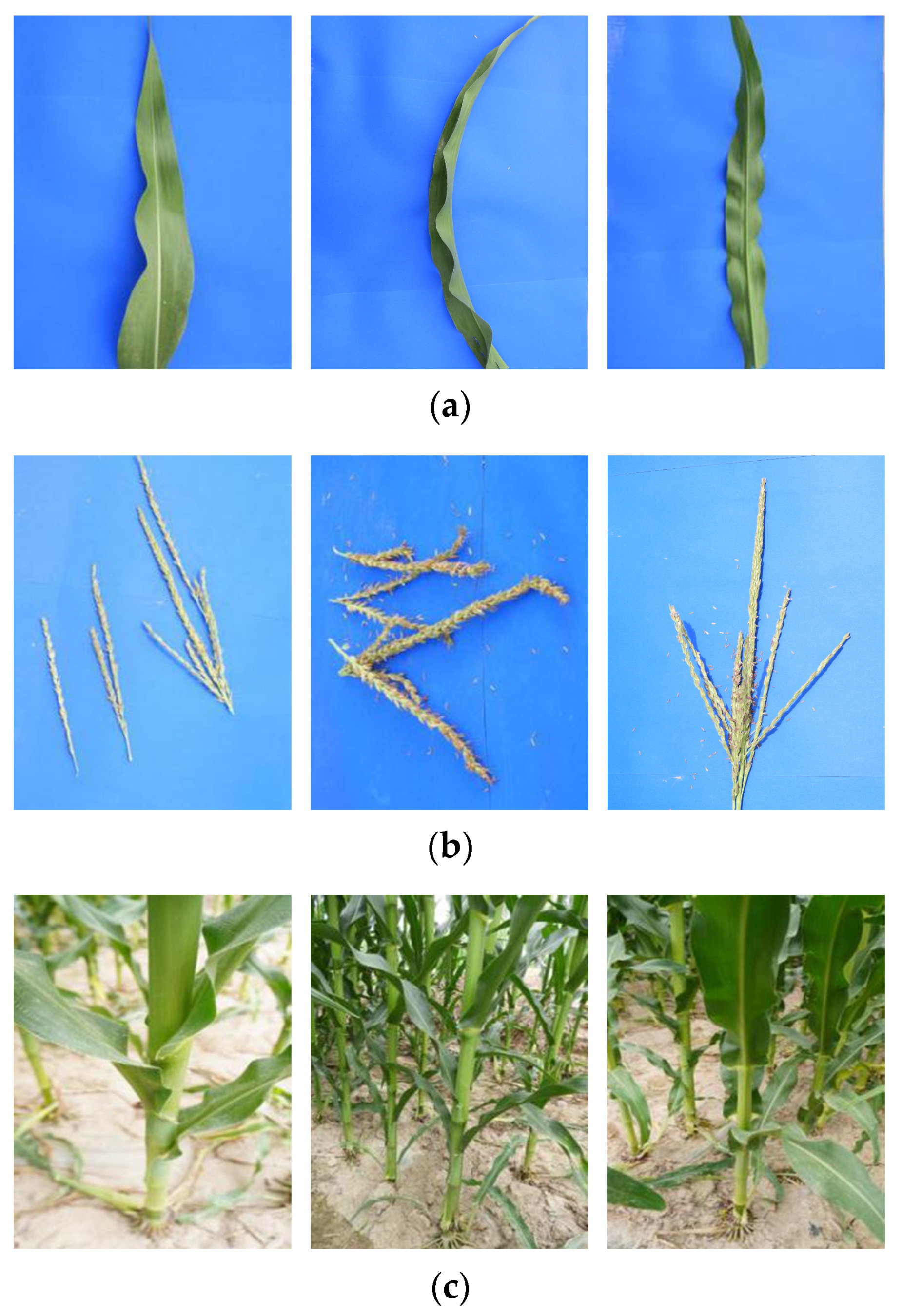
• Data collection and pre-processing: We collected images of leaves, staminates, and root caps of 40 corn varieties in Gansu Province at the nodulation stage and ensured the quality and usability of the data through image pre-processing and screening techniques, which provided high-quality data support for model training.
• Model optimization: We introduced the Representative Batch Normalization (RBN) structure into the DenseNet121 network model, which improves the generalization ability of the model under different data distributions and batch sizes.
• Structure optimization and feature extraction: Combining the advantages of the SE module and deep separable convolution improves the feature expression ability of the model, while reducing the computational cost, decreasing the model complexity, and ensuring high efficiency.
• Regularization and generalization ability: By introducing dropout regularization, the risk of overfitting of the model is reduced and the robustness on new data is improved.

Through these optimizations, we propose a lightweight convolutional neural network model for corn fertility identification, aiming to provide a new technological solution for corn variety identification that can be effectively deployed on low-computing power devices in the field.

2. Materials and Methods

2.1. Experimental Materials and Processing

2.1.1. Image Acquisition

All the corn image datasets in this study were collected in the corn Germplasm Innovation and Genetic Breeding Experimental Area of the Modern Agricultural Science and Technology Park of the Gansu Provincial Academy of Agricultural Sciences (38°56′ N, 100°26′ E, with an average elevation of 1482.7 m, an average annual rainfall of 129 mm, and an annual sunshine hour of 3085 h). Figure 1 shows a multi-angle and multi-scale photograph of the staminates, leaves, and cap roots of a corn plant under natural light outdoors using a Nikon COOLPIX B700 digital camera produced by Nikon Corporation in Tokyo, Japan (ISO 1600, shutter speed 1/30 s) and a cellular phone (Android 14, HDR auto mode), with an image format of JPG. The images were collected from 9 July to 13 July 2024, including three days of sunny days and two days of light rain. The image capture covered different weather, light and background conditions, and a total of 31,000 images of 40 corn varieties (

Table 1. Variety (series).

Range		Breed (Line)		Blade Image	Staminate Image	Root Cap Image
Hybrids	LD632	LD633	LD635	450	150	300
	LD635	LD655	LD656
	LD657	LD659	LD636
	LD2463	LD24159	LD634
	XY1483	XY335	XY698
	XY1620	XY1516	R1831
	RP909	DF899
Parent	Parent 1	Parent 2	Parent 3	300	150	200
	Parent 4	Parent 5	Parent 6
	Parent 7	Parent 8	Parent 9
	Parent 10	Parent 11	Parent 12
	Parent 13	Parent 14	Parent 15
	Parent 16	Parent 17	Parent 18
	Parent 19	Parent 20

), including 40 plants of each of 20 hybrid varieties and 20 plants of each of 20 parental varieties, covering multiple parts of the plant. The dataset was divided into training, validation, and test sets in the ratio of 7:2:1.

2.1.2. Image Processing

In deep learning algorithms, the quality of the dataset is critical to the training of network models and prediction performance. In order to improve the generalization ability and robustness of the network model, the size of the images in the training set and the verification set is adjusted to a square shape of 224 × 224 pixels, ensuring that all images have the same size. Each image in the training set is randomly horizontally flipped with a probability of 0.5 to increase the diversity of the training data and help the model become more robust and invariant to horizontal flipping. Min-max normalization is a method of rescaling data to a specific range [0, 1]. This rescaling can be achieved through a simple linear transformation that adjusts the raw data values to a uniform scale, enhancing algorithm stability and performance. The formula for min-max normalization [23] is depicted in Equation (1), where Nnorm represents the normalized image pixel value; x_i represents the pixel value of the input image.

$$Nnorm={\displaystyle \frac{x_i-\min (x)}{\max (x)-\min (x)}}$$

(1)

This conversion ensures that the contributions of all input features to model learning are balanced and avoids deviations caused by differences in original data scales.

2.2. Basic Methodology and Test Environment

2.2.1. Contrast Model

The experimental process of this research uses DenseNet [24] as the basic model. Each dense block consists of multiple convolutional layers, and these layers are spliced with their feature maps through direct connections. Specifically, each layer receives the feature maps of all previous layers as inputs, a design that effectively transfers gradients, and promotes feature reuse. As shown in Figure 2, the densely connected structure improves feature transfer efficiency, accelerates network convergence, and reduces the problem of gradient disappearance and explosion. This mechanism allows DenseNet to more effectively capture complex features and maintain the flow of information across the deep network.

In order to comprehensively evaluate the performance of the improved model in corn growth period classification, VGG16 [25], MobileNet V3 [26], ResNet50 [27], and ConvNeXt [28] were selected as comparison models. VGG16 is a classic deep convolutional network that can extract high-level features of images, but it requires a large amount of computation and takes a long training time. MobileNet V3 uses lightweight deeply separable convolution, which reduces computational complexity and is suitable for resource-limited environments. ResNet50 solves the gradient disappearance problem through residual connection, enhancing deep feature learning capabilities. ConvNeXt combines the advantages of traditional convolutional networks and transformers to provide powerful feature extraction capabilities.

Through these comparisons, we can evaluate the performance of different models in corn growth period classification from aspects such as accuracy, convergence speed, and calculation efficiency, thereby verifying the advantages of the improved model and providing reference for practical applications.

2.2.2. Evaluation Metrics

In this study, objective evaluation criteria were used to assess the established model for cornblade variety detection through Accurary (A), Precision (P), and Recall (R), and the F1 value was introduced as an average evaluation of the reconciliation [29]. Among them, the accuracy rate is used to measure the proportion of the model correctly classified; the accuracy rate reflects the accuracy of the model in predicting positive samples, especially for scenarios that focus on false positives; the recall rate evaluates the true positive samples captured by the model. The proportion of samples, especially when focusing on false negatives, is of great significance. In addition, the F1 value, as a harmonious average of accuracy and recall, can comprehensively consider the balance of these two indicators, especially when data are unbalanced, providing a more comprehensive evaluation of model performance. See

Table 2. Evaluation metrics formula comparison table.

Indicator	Formula
Accuracy (A)	$\mathrm{A}={\displaystyle \frac{\mathrm{T}\mathrm{P}+\mathrm{T}\mathrm{N}}{\mathrm{T}\mathrm{P}+\mathrm{T}\mathrm{N}+\mathrm{F}\mathrm{N}+\mathrm{F}\mathrm{P}}}\times 100\%$
Precision (P)	$\mathrm{P}={\displaystyle \frac{\mathrm{T}\mathrm{P}}{\mathrm{T}\mathrm{P}+\mathrm{F}\mathrm{P}}}\times 100\%$
Recall (R)	$\mathrm{R}={\displaystyle \frac{\mathrm{T}\mathrm{P}}{\mathrm{T}\mathrm{P}+\mathrm{F}\mathrm{N}}}\times 100\%$
F1	$\mathrm{F}1={\displaystyle \frac{2\mathrm{P}\mathrm{R}}{\mathrm{P}+\mathrm{R}}}\times 100\%$

for relevant formulas.

Where (TP) denotes the number of samples that are true positive cases and predicted as positive by the model; (FP) denotes the number of samples that are true negative cases but incorrectly predicted as positive by the model; (FN) denotes the number of samples that are true positive cases but incorrectly predicted as negative by the model; and (TN) denotes the number of samples that are true negative cases and predicted as negative by the model.

2.2.3. Test Environment

The experimental environment was Windows 10, 64-bit operating system, x64-based processor, Cuda version 11.0, and the Pytorch deep learning framework based on the Python programming language. The computer contains an NVIDIA GeForce MX150 graphics card produced by NVIDIA Corporation in Santa Clara, California.With 24 Gigabytes of video memory and a 1.80 GHz 8th generation Intel(R) Core(TM) i7-8550 CPU processor produced by Intel Corporation, Santa Clara, California, USA.

3. Model Improvements

3.1. Improving the DenseNet Model

3.1.1. Representative BatchNorm (RBN)

Gao [30] humanRepresentative BatchNorm (RBN) is an improved batch normalization method designed to enhance the training effectiveness and performance of deep neural networks. The traditional BatchNorm normalizes by computing the mean and variance on each training batch, and these statistics are based on the current small batch of data. However, this approach can be affected by the statistical noise of small batches of data. RBN introduces more representative statistics for normalization. These statistics not only consider the current small batch of data, but also incorporate statistical information from the historical training process. Specifically, RBN smoothens the mean and variance through a sliding average strategy to provide a more stable estimate of the overall data distribution. This approach mitigates the instability of the statistics of small batches of data and ensures the consistent performance of the network during the training and inference phases.

RBN consists of two main steps: centering calibration and scalar calibration, in a process as in Equation (2). In this phase of centering calibration, RBN normalizes the features so that their means are closer to the target mean. This is performed by introducing an additional representative mean parameter that aligns the mean of the features to the desired mean, thus reducing the bias during training. In the scale calibration step, RBN adjusts the variance of the features to ensure that their distribution is closer to the target variance. This is achieved by introducing a representative variance parameter so that the variance of the features is appropriately adjusted to improve the stability and generalization of the model. Through these two steps, RBN not only improves the normalization process of the features, but also enhances the performance of the model in the training and inference phases, adapting to different data distributions and task requirements, thus improving the flexibility and robustness of the model.

Centering Calibration:

$$X_{\mathrm{cm}}=X+w_m{K}_m$$

Centering:

$$X_{\mathrm{m}}=X_{cm}-E\left(X_{cm}\right)$$

Resizing:

$$X_{\mathrm{s}}={\displaystyle \frac{X_m}{\sqrt{Var\left(X_{cm}\right)+\epsilon }}}$$

(2)

Zoom Calibration:

$$X_{cs}=X_{s}R\left(w_v{K}_s+w_b\right)$$

Affine:

$$Y=X_{cs}\gamma +\beta$$

where input features X ∈ RN × C × H × W, w_m, w_v, w_b are learnable weight vectors. k_m and K_s represent the feature statistics for each instance, which can be obtained using global average pooling. R() is a constraint function that is often used with a Sigmoid. E(X) and Var(X) denote the mean and variance, which are used for centering and scaling. γ and β denote the scaling and bias factors of the Affine transformation, and ε is used to avoid zero variance. The crop features can be better recognized by replacing the original BN in DenseNet 121 with RBN, and this was experimentally validated.

3.1.2. SE Attention Mechanism

The attention mechanism mimics the focal attention in human vision or thinking, enabling the model to automatically learn to focus on specific parts of the input data and dynamically weight the feature information in the region of interest, thus efficiently utilizing the limited computational resources [31]. The SE Attention Mechanism Module [32] (shown in Figure 3) firstly compresses the feature maps of each convolutional layer into a single channel through global average pooling descriptor to capture global feature information. Next, the weights of each channel are generated using two fully connected layers and the ReLU activation function. Finally, these weights are normalized to between 0 and 1 by a Sigmoid activation function. These weights adjust the response of each channel of the original feature map, thereby increasing the sensitivity to important features while suppressing irrelevant features and improving the overall performance of the model.

The forward process of the SE (Squeeze-and-Excitation) attention mechanism is as follows: first, the spatial information of each channel is compressed into a channel descriptor of size C by global average pooling for the input feature maps of size H × W × C. Next, channel weights are generated through two fully connected layers. Specifically, the descriptor is first downscaled through a fully connected layer of size C/R (where r is the compression rate) and the intermediate representation is obtained using the ReLU activation function. Then, the intermediate representation is mapped back to the original number of channels C through a fully connected layer and the weights for each channel are obtained using the Sigmoid activation function. Ultimately, these weights are used to adjust the channel response of the original feature map.

Compression (Squeeze): the input feature map x is globally average pooled to obtain the channel descriptor z. The channel descriptor z is then used to adjust the channel response of the original feature map:

$$z=F_{pool}\left(x\right)\in R^C$$

(3)

Excitation: The descriptor z is mapped to an intermediate space using a fully connected layer and processed through the ReLU activation function. Next, a second fully connected layer is used to map the intermediate representation back to the original number of channels and generate the channel weights via a Sigmoid activation function.

$$z_{fc1}=\mathrm{Re}LU\left(W_{fc1}z+b_{fc1}\right)\in R^{{\displaystyle \frac{C}{r}}}$$

(4)

Channel weighting: the generated channel weights, sigma, are reshaped and applied to the original feature map, x:

$$\delta =\mathrm{Sigmoid}\left(W_{fc2}{z}_{fc1}+b_{fc2}\right)\in R^C$$

(5)

$$\mathrm{output}=x\times \delta$$

(6)

where W_fc1 and W_fc2 are the weight matrices of the fully connected layer, and b_fc1 and b_fc2 are the bias terms. This approach enables the SE module to adaptively adjust the weights of each channel, thus strengthening useful features and suppressing useless features, improving the feature representation, and final performance of the network. In order to verify the effectiveness of the SE module, we conducted comparison experiments of SE, ECA, and CBAM attention mechanisms. The results are shown in

Table 3. Attention performance comparison.

Attention Mechanism	Accuracy (%)	Precision (%)	Recall (%)	F1 Score (%)
ECA	89.89	90.68	89.88	89.95
CBAM	91.71	91.84	91.51	91.45
SE	94.81	95.04	94.66	94.67

. Adding the SE attention mechanism significantly improves the overall detection performance of the network.

3.1.3. Depth Separable Convolution

Depth separable convolution, proposed by Howard et al. [33] in 2017, is a typical lightweight convolution structure. Compared with standard convolution, it significantly reduces the number of parameters, improves the training speed, and allows separation of channels and regions during convolution operations. As shown in Figure 4, depth-separable convolution is a convolution operation that splits the traditional convolution operation into two separate steps: depth convolution and point-by-point convolution. In deep convolution, each input channel is processed through a separate convolution kernel to generate an output channel equal to the number of input channels. Point-by-point convolution, on the other hand, uses a convolution kernel of size 1 × 1 to manipulate the output of the deep convolution in order to integrate and compress the channel information to produce the final output feature map. This approach adjusts the number of channels without changing the spatial dimensions of the feature map, thus motivating the network to learn more complex feature representations.

Compared to traditional convolution methods, depth-separable convolution reduces the number of parameters by significantly reducing the computational cost while maintaining the performance of the model. The NH × W × C convolution kernel can be replaced by CH × W × 1 depth convolution and N1 × 1 × C point-by-point convolution. The number of parameters for deep convolution is (H × W × 1) × C and the number of parameters for point-by-point convolution is (1 × 1 × C) × N. The number of parameter combinations for the deep separable convolution is calculated as follows:

$$Params=H\times \mathrm{W}\times \mathrm{C}+\mathrm{C}\times \mathrm{N}$$

(7)

The number of parameters for ordinary convolution is H × W × C × N. The relationship between the two is compared as follows:

$${\displaystyle \frac{H\times \mathrm{W}\times \mathrm{C}+\mathrm{C}\times \mathrm{N}}{H\times \mathrm{W}\times \mathrm{C}\times \mathrm{N}}}={\displaystyle \frac{1}{N}}+{\displaystyle \frac{1}{\mathrm{H}\times \mathrm{W}}}$$

(8)

Comparison of the parameters of DenXt with the original DenseNet 121 model after using depth separable convolution instead of the original convolution is shown in

Table 4. Parameter comparison.

Model	Total Parameters	Trainable Parameters	Model Parameters (MB)
Densenet 121	6,994,856	6,994,856	20.68
DenXt	5,276,664	5,276,664	20.13

. The original DenseNet 121 model uses as many as 6,994,856 parameters, after depth separable convolution replacement this number is reduced by 1,718,192, and has smaller model parameters, which is favorable for lightweight network design. It also enhances the overall performance of the model.

3.1.4. Dropout

Dropout is a regularization technique proposed by Hinton et al. [34] in 2014 to prevent overfitting of neural networks. Compared with traditional regularization methods, Dropout is easier during model training and significantly improves the model’s ability to generalize to new data. As shown in Figure 5, dropout achieves regularization by randomly “dropping” some neurons in each training iteration. During training, dropout sets the output of some neurons to zero with a certain probability (e.g., 50%) to reduce the network’s dependence on specific neurons. During the testing phase, all neurons participate in the computation, but their activation values are scaled according to the dropout probability during the training phase. In this way, dropout enhances the robustness and generalization of the network without adding additional computational complexity.

3.2. The DenXt Model

The model focuses on improving the dense block structure in DenseNet in three ways, while the rest of the model remains consistent with DenseNet. In our improved DenseNet model, three key blocks are added: Squeeze-and-Excitation Block (SEBlock), Depth Separable Convolution (DS Conv), Representative Batch Normalization (RBN), and Dropout Layer to form the entire DenXt model, as shown in Figure 6. SEBlock improves feature representation by adaptively adjusting channel weights, Deep Separable Convolution improves efficiency by reducing computational complexity and model parameters, and Representative Batch Normalization simplifies processing in evaluation mode. These improvements result in significant gains in computational efficiency, memory usage, and generalization over traditional DenseNet. In addition, the model also supports overfitting prevention via dropout, which improves the generalization ability of the model. Overall, these improvements make our DenseNet model outperform the traditional DenseNet in terms of computational efficiency, memory usage and generalization ability, and achieve higher performance and efficiency.

Table 5. Detailed structural comparison.

Layer Type	DenseNet121	DenXt	Improvement
Conv Layer	7 × 7 Conv, stride = 2, BN-ReLU	7 × 7Conv, stride = 2, RBN	RBN combines ReLU and BatchNorm to enhance stability and speed up training.
Pooling	Maxpool, 3 × 3, stride = 2	Maxpool, 3 × 3, stride = 2	-
Dense Block1	BN-ReLU Conv1, BN-ReLU Conv2 (6x)	ReLU-RBN Conv1, ReLu-RBN-SE, ReLU-RBN Conv2 (6x)	The introduction of RBN and SEBlock for feature recalibration helps to learn important features.
Transition Layer1	BN-ReLU 1 × 1 Conv, Maxpool 2 × 2	RBN-ReLU 1 × 1 Conv, Maxpool 2 × 2	Apply RBN to 1 × 1 convolution to stabilize training.
Dense Block2	BN-ReLU Conv1, BN-ReLU Conv2 (12x)	ReLU-RBN Conv1, ReLu-RBN-SE, ReLU-RBN Conv2 (12x)	The introduction of RBN and SEBlock for feature recalibration helps to learn important features.
Transition Layer2	BN-ReLU 1 × 1 Conv, Maxpool 2 × 2	RBN-ReLU 1 × 1 Conv, Maxpool 2 × 2	Apply RBN to 1 × 1 convolution to stabilize training.
Dense Block3	BN-ReLU Conv1, BN-ReLU Conv2 (24x)	ReLU-RBN Conv1, ReLu-RBN-SE, ReLU-RBN Conv2 (24x)	The introduction of RBN and SEBlock for feature recalibration helps to learn important features.
Transition Layer3	BN-ReLU 1 × 1 Conv, Maxpool 2 × 2	RBN-ReLU 1 × 1 Conv, Maxpool 2 × 2	Apply RBN to 1 × 1 convolution to stabilize training.
Dense Block4	BN-ReLU Conv1, BN-ReLU Conv2 (16x)	ReLU-RBN Conv1, ReLu-RBN-SE, ReLU-RBN Conv2 (16x)	Combining RBN and SEBlock to further refine the features in the final dense block.
Classification Layer	7 × 7 global average pool, 1024D fully conected, softmax	7 × 7 global average pool, 1024D fully conected, softmax	-
Dropout	-	Applied after each Dense Block (6x, 12x, 24x, 16x)	Dropout prevents overfitting by randomly discarding units during training.

shows a detailed architectural comparison between DenXt and the original DenseNet121.

4. Results and Discussion

4.1. Ablation Experiments and Comparative Analysis

The ablation experiments demonstrate the effectiveness of a series of improvements to the DenseNet model. Test set accuracy and F1Score were used as metrics. The ablation experiments include the effect of the model after using only the RBN module, the SE Attention Mechanism module, the Depth Separable Convolution module, and the use of Dropout, as well as the effect of the final model. Modifications were made to the Dense Block of DenseNet. When the RBN module is used, the model is named Den-RBN; when the SE module is used, the model is named Den-SE, when the depth-separable convolution is used, the model is named Den-DW, and when the Dropout is used, the model is named Den-Drop. Combining the advantages of the improved model, the final model is named DenXt. The results of the ablation experiments on the test set are shown in

Table 6. Ablation study results (√: select module).

Model	Improvement Methods				Acc (%)	F1 (%)
	Representative BatchNorm	Squeeze and Excitation	Depthwise Separable Convolution	Dropout
Densenet 121					94.55	94.19
Den-RBN	√				95.01	94.97
Den-SE		√			94.81	94.67
Den-DS			√		96.54	96.50
Den-Drop				√	94.89	94.66
DenXt	√	√	√	√	97.79	97.75

. From Table 6, it can be seen that the improved Den-RBN, Den-SE, Den-DS, Den-Drop, and DenXt all have a better accuracy and F1Score compared to the DenseNet 121 model. Den-RBN, which is obtained through the introduction of the representative batch normalization, has a better accuracy and F1Score for this unit compared to the pre-modified DenseNet-121 on the test set by 0.46 percentage points in accuracy and 0.78 percentage points in F1Score; Den-SE by 0.26 percentage points in accuracy and 0.5 percentage points in F1Score on the test set; Den-DW by 1.99 percentage points in accuracy and 2.31 percentage points in F1Score on the test set; and Den-Drop improved its accuracy on the test set by 0.34 percentage points and its F1Score by 0.47 percentage points; the improved DenXt improved its accuracy on the test set by 3.24 percentage points and its F1 Score by 3.56 percentage points.

4.2. Analysis of Classification Results

The improved DenXt model was evaluated using the test dataset, and Figure 7 shows the confusion matrix of the improved DenXt model for classifying the appearance of corn varieties in the test set. The blade, staminate, and root cap morphology of the corn plants are very close, and the differences are subtle. So there are some recognition errors. Analyzed in terms of accuracy, precision, recall, and F1 value, all varieties (lines) were above 95.45%, 94.29%, 95.45%, and 95.45%, respectively, and these results indicate that there is a significant difference in model performance among different varieties (lines), and also indicate that the improved model performs well on the corn blade dataset, and is able to efficiently make the majority of varieties (lines) differentiate.

4.3. Comparison with Other Models

In order to better evaluate the performance of the improved DenXt network in this paper, the accuracy, precision, recall, F1 value, parameter size, and GPU memory evaluation values of the model are used as metrics for the comparison experiments with DenseNet 121, VGG16, MobileNet V3, ResNet50, and ConvNeXt network models in

Table 7. Evaluation metrics for different models.

Model	Accuracy/%	Precision/%	Recall/%	F1 Score/%	Parameters Size (MB)	GPU Memory (MB)	Inference Time (ms)
DenseNet 121	94.55	94.48	94.20	94.19	26.08	27.11	28,774.34
VGG16	89.45	89.67	89.23	89.19	512.79	513.66	13,243.09
MobileNet V3	89.49	89.34	88.99	88.91	16.22	16.40	2407.02
ResNet50	92.69	92.91	92.30	92.30	90.02	90.29	2661.37
ConvNeXt	94.49	94.46	94.23	94.23	748.79	749.67	3413.79
DenXt	97.79	97.27	97.75	97.75	20.13	20.62	2265.95

. The classification accuracies of different models on the test set are shown in Figure 8, where the improved DenXt model achieves an average accuracy of 97.79% on the test set, which is an improvement of 3.3 to 8.34 percentage points over the other models, and an average precision of 97.77%, which is an improvement of 3.31 to 8.1 percentage points over the other network models. Similarly, the average recall was improved by 3.52 to 8.52 percentage points to 97.75% over other models, while the F1 score value reached 97.75%, which was improved by 3.52 to 8.56 percentage points over other models. In contrast, the other models showed lower accuracy in classifying image samples of corn plant varieties. Although lightweight models such as MobilenetV3 (with parameters of only 16.22 MB) have some advantages in terms of memory footprint and computational efficiency, their accuracy and other evaluation metrics (e.g., Precision, Recall, and F1 Score) are significantly lower than those of DenXt. DenXt’s performance on Precision and Recall is also better than these lightweight models, indicating that it not only outperforms other small models in terms of overall accuracy, but is also more precise and comprehensive in handling classification tasks. At the same time, DenXt’s reasoning time (2265.95 ms) is also better than other models, especially Densenet 121 (28,774.34 ms) and VGG16 (13,243.09 ms). Its lower latency makes it particularly outstanding in scenarios with high real-time requirements. These findings provide evidence for the superior performance of the model proposed in this paper.

4.4. Network Visualization

In order to better observe the learning ability of the DenXt model for corn plant features at the elongation stage, we used Grad-CAM to visualize corn leaves, staminates, and root caps. In this study, we chose the last layer of the DenXt model as the feature visualization layer of the network for feature visualization, as shown in Figure 9. By observing the visualization results, we found that the DenXt model accurately identifies the key regions of different parts. In addition, we noticed that the model pays less attention to irrelevant and complex backgrounds such as the soil around the plant. Thus, these results validate the strong learning ability of the DenXt model for plant characteristics during the corn uprooting stage.

5. Conclusions and Outlook

This study aims to address the challenges in corn variety classification during the reproductive stage and achieves this goal by developing an efficient convolutional neural network (CNN) model. We first collected and preprocessed blade, male cob, and root cap images of 40 corn varieties in Gansu Province at the elongation stage to ensure the quality and representativeness of the data and to provide a reliable basis for model training. In terms of model improvement, we introduced the Representative Batch Normalization (RBN) structure in the DenseNet-121 network, and this improvement enhanced the generalization ability of the model under different data distributions and batch sizes, making the feature distribution more stable. In order to enhance the model’s focus on channel information, we integrate the SE module and depth-separable convolution, which not only improves the feature representation capability, but also effectively reduces the computational time cost and model complexity. In addition, the introduction of dropout regularization effectively reduces the risk of overfitting, and by randomly “dropping” some neurons, the model avoids overdependence on the training data during the training process, which improves the extensiveness of the feature learning and the robustness of the model. The proposed DenXt network model outperforms other popular image classification models, including VGG16, MobileNet V3, ResNet50, and ConvNeXt, while maintaining low model complexity. Compared with the original network model, the accuracy of our DenXt network model is improved by 3.23% and the parameter counts are reduced by 32.56%. In summary, the proposed new method shows good performance in the application of corn variety identification at the pulling out stage, which demonstrates the feasibility of deploying it for use in low-computing power smart farm equipment platforms in the field.

References

1. Food and Agriculture Organization of the United Nations (FAO). FAOSTAT Database. 2023. Available online: https://www.fao.org/faostat/en/#home (accessed on 20 August 2024).
2. Edmeades, G.O.; Trevisan, W.; Prasanna, B.M.; Campos, H. Tropical maize (Zea mays L.). In Genetic Improvement of Tropical Crops; Springer: Cham, Switzerland, 2017; pp. 57–109. [Google Scholar]
3. Erenstein, O.; Jaleta, M.; Sonder, K.; Mottaleb, K.; Prasanna, B.M. Global maize production, consumption and trade: Trends and R&D implications. Food Secur. 2022, 14, 1295–1319. [Google Scholar]
4. Guerra, A.; Scremin-Dias, E. Leaf traits, sclerophylly and growth habits in plant species of a semiarid environment. Braz. J. Bot. 2018, 41, 131–144. [Google Scholar] [CrossRef]
5. Chen, F.; Liu, J.; Liu, Z.; Chen, Z.; Ren, W.; Gong, X.; Wang, L.; Cai, H.; Pan, Q.; Yuan, L.; et al. Breeding for high-yield and nitrogen use efficiency in maize: Lessons from comparison between Chinese and US cultivars. Adv. Agron. 2021, 166, 251–275. [Google Scholar]
6. Ganesh, A.; Shukla, V.; Mohapatra, A.; George, A.P.; Bhukya DP, N.; Das, K.K.; Kola, V.S.R.; Suresh, A.; Ramireddy, E. Root cap to soil interface: A driving force toward plant adaptation and development. Plant Cell Physiol. 2022, 63, 1038–1051. [Google Scholar] [CrossRef] [PubMed]
7. Kamilaris, A.; Prenafeta-Boldú, F.X. Deep learning in agriculture: A survey. Comput. Electron. Agric. 2018, 147, 70–90. [Google Scholar] [CrossRef]
8. Tiwari, V.; Joshi, R.C.; Dutta, M.K. Dense convolutional neural networks based multiclass plant disease detection and classification using leaf images. Ecol. Inform. 2021, 63, 101289. [Google Scholar] [CrossRef]
9. Laabassi, K.; Belarbi, M.A.; Mahmoudi, S.; Mahmoudi, S.A.; Ferhat, K. Wheat varieties identification based on a deep learning approach. J. Saudi Soc. Agric. Sci. 2021, 20, 281–289. [Google Scholar] [CrossRef]
10. Oikonomidis, A.; Catal, C.; Kassahun, A. Deep learning for crop yield prediction:a systematic literature review. N. Zeal. J. Crop Hortic. Sci. 2023, 51, 1–26. [Google Scholar] [CrossRef]
11. Wang, Z.; Huang, W.; Tian, X.; Long, Y.; Li, L.; Fan, S. Rapid and non-destructive classification of new and aged maize seeds using hyperspectral image and chemometric methods. Front. Plant Sci. 2022, 13, 849495. [Google Scholar] [CrossRef]
12. Hinton, G.E.; Salakhutdinov, R.R. Reducing the dimensionality of data with neural networks. Science 2006, 313, 504–507. [Google Scholar] [CrossRef]
13. Rasti, S.; Bleakley, C.J.; Silvestre, G.C.; Holden, N.M.; Langton, D.; O’Hare, G.M. Crop growth stage estimation prior to canopy closure using deep learning algorithms. Neural Comput. Appl. 2021, 33, 1733–1743. [Google Scholar] [CrossRef]
14. Anami, B.S.; Malvade, N.N.; Palaiah, S. Deep learning approach for recognition and classification of yield affecting paddy crop stresses using field images. Artif. Intell. Agric. 2020, 4, 12–20. [Google Scholar] [CrossRef]
15. Song, Z.; Wang, P.; Zhang, Z.; Yang, S.; Ning, J. Recognition of sunflower growth period based on deep learning from UAV remote sensing images. Precis. Agric. 2023, 24, 1417–1438. [Google Scholar] [CrossRef]
16. Xu, J.; Wang, J.; Xu, X.; Ju, X. Rice growth stage image recognition based on RAdam convolutional neural network. Trans. Chin. Soc. Agric. Eng. 2021, 37, 143–150. [Google Scholar]
17. Liu, P.; Liu, L.; Wang, C.; Zhu, Y.; Wang, H.; Li, X. Method for determining the flowering stage of wheat in the field based on machine vision. J. Agric. Mach. 2022, 53, 251–258. [Google Scholar]
18. Han, Y.; Xing, H.; Jin, H. Design of an automatic detection system for maize seedling emergence and three-leaf stage based on OpenCV. J. Electron. Meas. Instrum. 2017, 31, 1574–1581. [Google Scholar] [CrossRef]
19. Zhang, Y.; Liu, R.; Liu, M.; Gong, Y. Recognition of maize growth stages based on deep convolutional features. Electron. Meas. Technol. 2018, 41, 79–84. [Google Scholar] [CrossRef]
20. Shi, L.; Lei, J.; Wang, J.; Yang, C.; Liu, Z.; Lei, X.; Xiong, S. A lightweight wheat growth stage recognition model based on improved FasterNet. J. Agric. Mach. 2024, 55, 226–234. [Google Scholar]
21. Zheng, G.; Wei, J.; Ren, Y.; Liu, H.; Lei, X. Research on a lightweight wheat growth monitoring model based on deep separable and dilated convolutions. Jiangsu J. Agric. Sci. 2022, 50, 226–232. [Google Scholar] [CrossRef]
22. Sheng, R.T.-C.; Huang, Y.-H.; Chan, P.-C.; Bhat, S.A.; Wu, Y.-C.; Huang, N.-F. Rice growth stage classification via RF-based machine learning and image processing. Agriculture 2022, 12, 2137. [Google Scholar] [CrossRef]
23. Mo, H.; Wei, L. SA-ConvNeXt: A hybrid approach for flower image classification using selective attention mechanism. Mathematics 2024, 12, 2151. [Google Scholar] [CrossRef]
24. Huang, G.; Liu, Z.; Van Der Maaten, L.; Weinberger, K.Q. Densely connected convolutional networks. In Proceedings of the IEEE Conference on Computer Vision and Pattern Recognition, Honolulu, HI, USA, 21–26 July 2017; pp. 4700–4708. [Google Scholar]
25. Yang, H.; Ni, J.; Gao, J.; Han, Z.; Luan, T. A novel method for peanut variety identification and classification by Improved VGG16. Sci. Rep. 2021, 11, 15756. [Google Scholar] [CrossRef]
26. Koonce, B.; Koonce, B. MobileNetV3. In Convolutional Neural Networks with Swift for Tensorflow: Image Recognition and Dataset Categorization; Apress: New York, NY, USA, 2021; pp. 125–144. [Google Scholar]
27. Mukti, I.Z.; Biswas, D. Transfer learning based plant diseases detection using ResNet50. In Proceedings of the 2019 4th International Conference on Electrical Information and Communication Technology (EICT), Khulna, Bangladesh, 20–22 December 2019; IEEE: Piscataway, NJ, USA, 2019; pp. 1–6. [Google Scholar]
28. Feng, J.; Tan, H.; Li, W.; Xie, M. Conv2NeXt: Reconsidering Conv NeXt Network Design for Image Recognition. In Proceedings of the 2022 International Conference on Computers and Artificial Intelligence Technologies (CAIT), Quzhou, China, 4–6 November 2022; IEEE: Piscataway, NJ, USA, 2022; pp. 53–60. [Google Scholar]
29. Xing, X.; Liu, C.; Han, J.; Feng, Q.; Lu, Q.; Feng, Y. Wheat-seed variety recognition based on the GC_DRNet model. Agriculture 2023, 13, 2056. [Google Scholar] [CrossRef]
30. Gao, S.H.; Han, Q.; Li, D.; Cheng, M.M.; Peng, P. Representative batch normalization with feature calibration. In Proceedings of the IEEE/CVF Conference on Computer Vision and Pattern Recognition, Nashville, TN, USA, 20–25 June 2021; pp. 8669–8679. [Google Scholar]
31. Mi, Z.; Zhang, X.; Su, J.; Han, D.; Su, B. Wheat stripe rust grading by deep learning with attention mechanism and images from mobile devices. Front. Plant Sci. 2020, 11, 558126. [Google Scholar] [CrossRef]
32. Hu, J.; Shen, L.; Sun, G. Squeeze-and-excitation networks. In Proceedings of the IEEE Conference on Computer Vision and Pattern Recognition, Salt Lake City, UT, USA, 18–23 June 2018; pp. 7132–7141. [Google Scholar]
33. Howard, A.G.; Zhu, M.; Chen, B.; Kalenichenko, D.; Wang, W.; Weyand, T.; Andreetto, M.; Adam, H. Mobilenets: Efficient convolutional neural networks for mobile vision applications. arXiv 2017, arXiv:1704.04861. [Google Scholar]
34. Srivastava, N.; Hinton, G.; Krizhevsky, A.; Sutskever, I.; Salakhutdinov, R. Dropout: A simple way to prevent neural networks from overfitting. J. Mach. Learn. Res. 2014, 15, 1929–1958. [Google Scholar]
Figure 1. Corn plant. (a) Blade. (b) Staminate. (c) Root cap.
Agriculture 15 00079 g001
Figure 2. DenseNet structure diagram.
Agriculture 15 00079 g002
Figure 3. SE Module.
Agriculture 15 00079 g003
Figure 4. Depthwise separable convolution.
Agriculture 15 00079 g004
Figure 5. Training process (From bottom to top, there are input layer, hidden layer 1, hidden layer 2, and output layer, where white means discarding neurons.).
Agriculture 15 00079 g005
Figure 6. DenXt network architecture diagram.
Agriculture 15 00079 g006
Figure 7. Confusion matrix.
Agriculture 15 00079 g007
Figure 8. Accuracy comparison.
Agriculture 15 00079 g008
Figure 9. Thermogram detection and analysis.
Agriculture 15 00079 g009