Abstract
This study presents an approach to address the challenges of recognizing the maturity stage and counting sweet peppers of varying colors (green, yellow, orange, and red) within greenhouse environments. The methodology leverages the YOLOv5 model for real-time object detection, classification, and localization, coupled with the DeepSORT algorithm for efficient tracking. The system was successfully implemented to monitor sweet pepper production, and some challenges related to this environment, namely occlusions and the presence of leaves and branches, were effectively overcome. We evaluated our algorithm using real-world data collected in a sweet pepper greenhouse. A dataset comprising 1863 images was meticulously compiled to enhance the study, incorporating diverse sweet pepper varieties and maturity levels. Additionally, the study emphasized the role of confidence levels in object recognition, achieving a confidence level of 0.973. Furthermore, the DeepSORT algorithm was successfully applied for counting sweet peppers, demonstrating an accuracy level of 85.7% in two simulated environments under challenging conditions, such as varied lighting and inaccuracies in maturity level assessment.
1. Introduction
Precision agriculture refers to a contemporary method of farming management that employs advanced technology to enhance crop yields, minimize resource wastage, and reduce environmental impact. This approach involves integrating technology into various aspects of agriculture to monitor, measure, and adapt to variations in crop conditions [1]. Precision agriculture aims to improve crop yields, reduce costs, and enhance sustainability by using resources more efficiently and reducing the environmental impact of farming practices. It is becoming an increasingly important field as the global population continues to grow, and there is a need for more efficient and sustainable food production [2].
Modern agriculture technology has made predicting crop yields a priority. This information is critical for farmers as it allows them to make informed decisions regarding seed quantities, fertilizers, and other resources. Precision in predicting crop yields enables farmers to increase profitability, optimize crop cultivation, and minimize waste. It also assists in their long-term planning by providing insights into prospective harvests and guiding crop selection and planting schedules [3]. Farmers can use various methods such as visual checks, sampling, remote sensors, fruit counting, and assessing greenhouse maturity levels to predict crop yields. These methods are crucial because they enable farmers to plan their harvests effectively and maximize their crop yields [4]. Computer vision is a technological advancement that allows computers to interpret images or videos captured through cameras or sensors. It has been used in estimating crop production by performing tasks such as plant counting, identifying various plant components, detecting disease, and evaluating maturity. Computer vision algorithms can accurately tally the number of plants within a field, assess the dimensions and forms of individual plants, and determine the total crop production for the entire area by analyzing high-resolution images of crops. These advantages assist farmers in receiving early alerts regarding possible issues that could affect their crop yield and taking measures promptly to stop the spread of diseases, thus preventing substantial damage to their crops. Fuzzy Logic, support vector machines, and convolutional neural networks (CNNs) are the latest technologies used for the maturity classification and counting of fruits. These methods can detect fruit maturity levels more accurately and quickly [5]. The effectiveness of maturity detection through object detection can vary, depending on the technique employed. Object recognition technology must accurately identify real-time information about characteristics such as sweet peppers’ color, size, and shape. These factors are critical in determining the yield level. Greenhouses are typically designed to optimize crop production, which can limit the placement of cameras and their field of view. Additionally, the appearance of sweet peppers varies as they progress through different stages of development, and the dense vegetation in greenhouses further complicates the issue [6].
In a recent study, Zhao et al. [7] proposed an automated technique for detecting ripe tomatoes in greenhouse environments that combines the AdaBoost classifier and color analysis. The method was tested on 150 positive and 683 negative samples, and it successfully identified over 96% of ripe tomatoes in real-world conditions. However, there was a 10% false-negative rate, meaning that 3.5% of tomatoes were undetected. Despite this, the proposed method remains a simple and practical approach for spotting ripe tomatoes in greenhouse environments. To automate tomato harvesting, G. Liu et al. [8] developed a system that uses Histograms of Oriented Gradients (HOG) and a support vector machine (SVM) to identify ripe tomatoes. The algorithm was tested on a dataset of 500 images with tomatoes and different background objects. The results showed 90.00% recall, 94.41% precision, and an F1 score of 92.15%, which significantly outperformed other advanced tomato detection algorithms. Liu et al. [9] also presented a method for automatically grading tomatoes based on color, shape, and size using machine vision to analyze tomato images and classification algorithms in order to determine maturity and size. The method achieved an accuracy of 90.7% when tested with a dataset of 350 tomato images, demonstrating its effectiveness in categorizing tomatoes based on their physical features. While rule-based algorithms can technically identify pepper maturity, they often involve complex decision making and require expensive equipment, resulting in slower identification rates.
Deep learning models, on the other hand, offer significant advantages, including high accuracy and the ability to generalize well across various conditions, addressing these challenges. Alajrami and Abu-Naser [10] suggested a way to use deep learning for automatically classifying types of tomatoes. The design included three convolutional layers, two pooling layers, and one fully connected layer. The outcomes demonstrated a classification accuracy of 93.2%. Long et al. [11] created a better Mask R-CNN model to accurately outline tomatoes in greenhouses. The model was built on the original Mask R-CNN but with improvements like a changed backbone network, altered pooling layer, and adjusted mask prediction. The model accurately identified ripe tomatoes in greenhouse images with 95.58% accuracy and 97.42% for the mean average precision (MAP). Long et al. [12] proposed a new network called SE-YOLOv3-MobileNetV1 to detect ripe tomatoes in greenhouses. This network improved accuracy by using mosaic data augmentation and K-means clustering. The network achieved a 95.58% accuracy rate and a 97.42% mean average precision in identifying ripe tomatoes. The model identified branch-occluded tomato images, leaf-occluded tomato images, and overlapping tomato images. The branches of tomatoes are larger and have fewer leaves than those of peppers, which means that the fruit is more exposed, making it is easier to detect. Moreira et al. [13] compared two deep learning models, SSD MobileNet v2 and YOLOv4, for their ability to detect tomatoes. YOLOv4 performed better, reaching the highest overall performance with an 85.51% F1 score for detection. In another study by Moon et al. [14], the authors proposed using a combination of convolutional and multilayer perceptron (CNN-MLP) to predict sweet pepper growth stages. Using images, the CNN identified fruits in three stages (immature, breaking, and mature). The MLP further broke down the immature stage into four sub-stages using plant and environmental data. When tested on 4000 sweet pepper images, the combined model reached an overall accuracy of 77%, performing better than using just a CNN or MLP alone. This highlights the strength of the combined approach. Dassaef et al. [15] used a dataset of more than 1400 images with manually annotated fruits and peduncles to detect fruits and stems of green sweet peppers in greenhouse environments. The study explored the use of Mask R-CNN, considering challenges such as occlusion, overlaps, and varying light conditions. The authors achieved a precision of 84.53% in fruit detection and 71.78% in peduncle detection, with an overall mean average precision (mAP) of 72.64% for instance segmentation. Following a similar approach, this project aims to detect fruit for harvesting and estimate yields. Seo et al. [16] introduced a robot monitoring system designed for tomato fruits in hydroponic greenhouses. This system employed machine vision to detect and track tomatoes while classifying their maturity levels. Operating in real time, it proved resilient to lighting conditions and background clutter changes. The system achieved an accuracy of 90% in detecting tomato fruits and an 88% accuracy in classifying their maturity levels.
On the other hand, in the counting process, feature extraction techniques for elements such as shape, texture, and changes in color space are employed to highlight the objects of interest [17]. Counting presents a challenge due to issues like inconsistent fruit detection and the potential for double counting. Detecting fruits reliably is tough due to variations in size, making it challenging to extract useful information. One common solution is using a multi-object tracking (MOT) algorithm to build global models containing all relevant objects in the environment. MOT is applied in agricultural and food settings for monitoring and fruit counting [18]. In their work, Rapado-Rincon et al. [19] employed a multi-view perception algorithm to detect and track tomatoes on plants from different angles. The results demonstrated that the method accurately located and reconstructed all tomatoes, even in challenging conditions. It estimated the total tomato count with a maximum error of 5.08%, achieving up to 71.47% tracking accuracy. Wojke et al. [20] introduced a DeepSORT technique to improve the data association abilities of basic tracking algorithms using the Kalman filter and the Hungarian algorithm. In their experiments, these additions reduced identity switches by 45%, showing competitive performance at high frame rates. DeepSORT employs a small convolutional neural network to extract features from identified objects, merging them with positional data to enhance tracking, especially in situations with occlusions. It has been successfully applied in agro-food environments. Kirk et al. [21] came up with a way to track strawberries as they grow using a feature extraction network. They upgraded the regular DeepSORT network by adding a classification head. This extra part learned to recognize different fruit IDs and ripeness stages at the same time. The authors found that adding the classification head improved the feature extractor network’s ability to connect and organize data. Villacrés et al. [22] provided a detailed comparison of tracking-by-detection algorithms for counting apples in orchards. The findings indicated that DeepSORT performed the best overall, boasting a mean average precision (mAP) of 93.00%. The Kalman filter also delivered strong results, with an mAP of 92.15%. The authors concluded that both DeepSORT and the Kalman filter are effective for accurately counting apples in orchards. Egi et al. [23] evaluated tracking-by-detection algorithms for counting apples in orchards and greenhouses using a UAV. DeepSORT obtained a 93.00% mean average precision (mAP), while the Kalman filter obtained an mAP of 92.15%. The authors suggested that both DeepSORT and the Kalman filter are effective for apple counting in orchards. Zhang et al. [24] introduced a deep-learning-based algorithm designed for detecting and tracking citrus fruits (oranges) in the field. This algorithm utilized the Orange YOLO model for citrus fruit detection in images and employed Orange Sort, a modified version of the SORT tracking algorithm, for fruit tracking over time. Achieving a 95.7% mean average precision for fruit detection and a 93.2% tracking accuracy, the system excelled in challenging conditions like occlusion and clutter. In the current literature, there are no works related to classifying the maturity levels of sweet peppers and tracking in greenhouse environments.
In this study, we developed a methodology to identify the maturity stage and track sweet peppers across their typical color variations (green, yellow, orange, and red). Our goal was to estimate the yield of these fruits in greenhouse production. We utilized YOLOv5 for detection, enabling the classification of sweet pepper maturity. Additionally, we integrated DeepSORT for counting, providing estimates of the pepper count in a greenhouse lane. To train and validate our algorithm, we gathered 1127 images from CAETEC (the Experimental Agricultural Field of the Tec de Monterrey). To ensure accurate fruit detection, our approach overcomes challenges like overlapping objects and changing obstacles such as leaves and branches. Importantly, due to environmental factors, our system can identify immature sweet peppers, particularly the most challenging color (green). This work aimed to enhance the maturity recognition and fruit counting of sweet peppers, which have not previously been reported in relation to the state-of-the-art application of YOLOv5 and DeepSORT.
The subsequent sections of this article are organized as follows: Section 2 introduces important concepts that are necessary to consider, such as basic knowledge of YOLOv5, the DeepSORT algorithm, evaluations metrics, and intersection over union (). Section 3 describes the experimental setup, while Section 4 presents the results. Lastly, in Section 5, conclusions and future work are presented.
2. Materials and Methods
2.1. Sweet Peppers
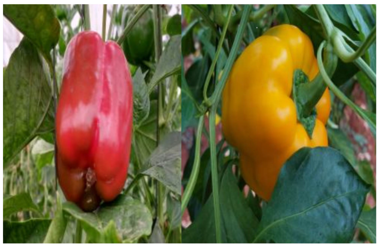
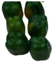
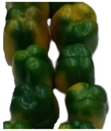
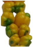
Sweet peppers, also known as bell peppers, paprika, or peppers, are the fruits of plants in the Grossum group of the species Capsicum annuum. Although botanically classified as fruits, they are usually considered vegetables in culinary terms. Sweet peppers come in a variety of colors, such as red, yellow, orange, green, white, chocolate, candy-cane striped, and purple, as shown in Figure 1. The color of the pepper indicates its ripeness, with red peppers being the ripest [25].
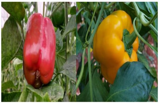
Figure 1.
Sweet peppers.
2.2. Greenhouse
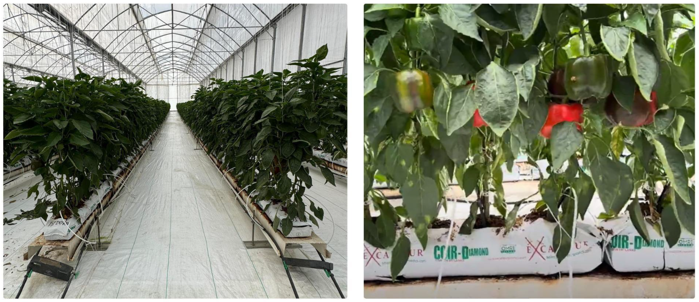
Greenhouses are structures that provide protection from different weather elements such as wind, rain, and snow. They also allow for the manipulation of growing conditions like temperature, humidity, and light levels. Greenhouses made of glass or plastic are commonly used to grow sweet peppers, with sloped roofs to allow rainwater runoff and insulated walls for temperature regulation. Sweet peppers can be grown year round in greenhouses regardless of the weather outside, making it possible to produce sweet peppers even in cold climates. The most common types of sweet bell peppers grown in greenhouses come in green, orange, yellow, and red varieties. Pests and diseases are a common threat to greenhouse plants and must be prevented. The greenhouse at CAETEC, where the images used for the algorithm’s training were obtained, is shown in Figure 2.

Figure 2.
(Left) Greenhouse at CAETEC, (right) mature sweet peppers.
2.3. Intel Real-Sense D435i
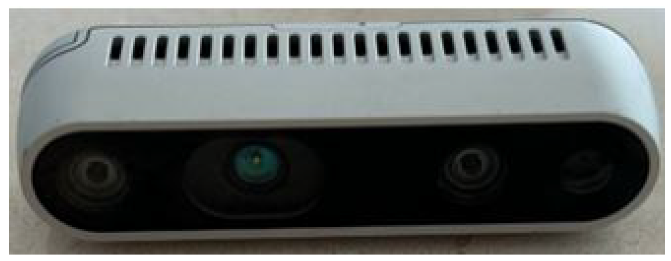
The D435i RGB-D camera (Intel, 2200 Mission College Blvd, Santa Clara, CA, USA) uses a projector to create a random, sharply focused infrared (IR) dot pattern. The camera also features right and left IR cameras, which enable it to capture and measure the distance between the projector’s output and the objects within its field of view (FOV), as illustrated in Figure 3. The depth is primarily determined by comparing the left and right video images recorded simultaneously and calculating the disparity for each pixel. Subsequently, the results are triangulated [26].
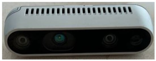
Figure 3.
Intel D435i camera.
The device measures 90 mm × 25 mm, weighs 258g, and can be used alone or integrated with a laptop or mobile device. See Table 1 for technical specifications [26].

Table 1.
Technical specifications.
The RealSense APIs allow direct access to internal and external camera sensor properties. Additionally, a wide range of external testing methods are available [27].
2.4. Evaluation Metrics
To evaluate the effectiveness of YOLOv5, we used the following five metrics: accuracy, precision, recall, , and mean average precision (). The classification outcomes were categorized into four groups: true positives (), which represent the number of correctly identified objects; true negatives (), indicating correct rejections; false positives (), which correspond to the number of incorrectly identified data points; and false negatives (), representing the number of missed objects [28].
Three analytical criteria were derived from these evaluation metrics, as defined by Equations (1)–(3): , , and .
A valid prediction algorithm is usually indicated by a high degree of proportionality between recall and precision [29]. The defined in Equation (4) combines precision and recall into a single metric. This metric is normally used to gauge the overall accuracy of a model. Additionally, the can be a valuable way to demonstrate how stable a model is. A higher value suggests that the model is more stable.
Mean average precision () combines precision and recall into a comprehensive metric. It takes the average of the “average precision” calculated for each class, as expressed in Equation (5):
where P stands for precision, while R represents recall, i represent the current class, and n indicates the total number of classes.
2.5. Intersection over Union
Imagine two boxes: one representing a prediction (e.g., where a model thinks an object is) and the other representing the ground truth (where the object actually is). The measures how much these two boxes overlap. Find the area where the two boxes overlap. This is the “intersection”. Combine the areas of both boxes, but only count overlapping areas once. This is the “union”. Divide the intersection area by the union area. This gives the score, a value between 0 and 1. An of 1 means a perfect overlap (the boxes are identical). An of 0 means no overlap at all. Higher scores generally indicate better object detection or tracking accuracy [30]. The metric, essential for this method, can be calculated using Equation (6).
The tracker depends largely on how well object detection models can spot objects. It is a very good object tracker because it is not computationally expensive and can handle frame rates of over 50,000 fps. By predicting with the Kalman filter, users can save time by not analyzing every frame. The detector can also save time and energy by skipping unnecessary frames and dealing with fewer overall images.
2.6. SORT Counting Algorithm
The SORT algorithm is an effective way to track objects in live videos. It uses the Kalman filter and the Hungarian algorithm to figure out where objects are and how fast they are moving in different frames. To track objects accurately, two algorithms work together. The Hungarian algorithm ensures correct identity assignment, preventing confusion across frames. The Kalman filter then predicts future positions by filtering out noise and jitters in the video data. SORT proves invaluable in the realm of computer vision, particularly in applications like surveillance, autonomous driving, and robotics. Its effectiveness shines in challenging scenarios, such as instances where objects obstruct each other, undergo appearance changes, or move at varying speeds. SORT is effective at tracking objects in real time, and it is popular because it is accurate, works fast, and can handle different situations well [20]. For a quick overview of the SORT algorithm, refer to the simplified summary provided in Figure 4.
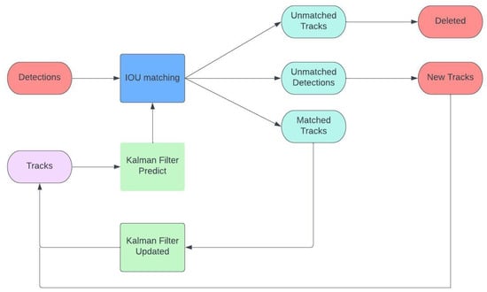
Figure 4.
Object tracking SORT algorithm diagram.
The SORT data association module compares the Kalman filter’s (KF) predicted bounding boxes with the image object detector’s measured bounding boxes. This component is essential to the SORT method because it improves real-time tracking efficiency by linking new detections to previously established object tracks. This component inputs the KF-obtained bounding boxes (N) and the forecasted bounding boxes (M). The module defines a linear assignment problem (, and , respectively) utilizing the intersection-over-union () metric. This is accomplished by creating a cost matrix that establishes the relationship between each detected bounding box and all expected bounding boxes.
The Hungarian method may be used to resolve this problem by reducing it to a minimization problem defined by the between the detected and anticipated bounding boxes:
After calculating the cost matrix, the Hungarian technique links the bounded regions. The resulting correlations are displayed as an N-by-M matrix, where M is the number of tracks and N is the number of measurements. Associations are filtered using a minimum threshold and a maximum threshold. Any connections with values below the cutoff are disregarded. In the KF estimation module, a linear constant velocity model represents each object’s motion. An item’s bounding box determines the track’s new state if linked to a tracked object. The state can only be anticipated if an item and a track’s condition cannot be connected. The tracking control component is responsible for adding and removing tracks. Additional tracks are generated when the value between two tracks is less than a certain threshold. The KF state is first set based on the detection’s bounding box. Since the item’s boundary is the sole information given, the KF has significant covariance and zero velocity for the object.
2.7. Artificial Neural Networks
2.7.1. Deep Learning
Today, the ML methodology that shows the most promise for detecting and localizing produce in very complex environments is deep learning (DL). DL is characterized by adding more complexity to a model, allowing it to represent data at multiple levels of abstraction [31]. These techniques excel at solving complex problems well and fast (through parallelization) if provided with adequately large datasets describing the problem [32].
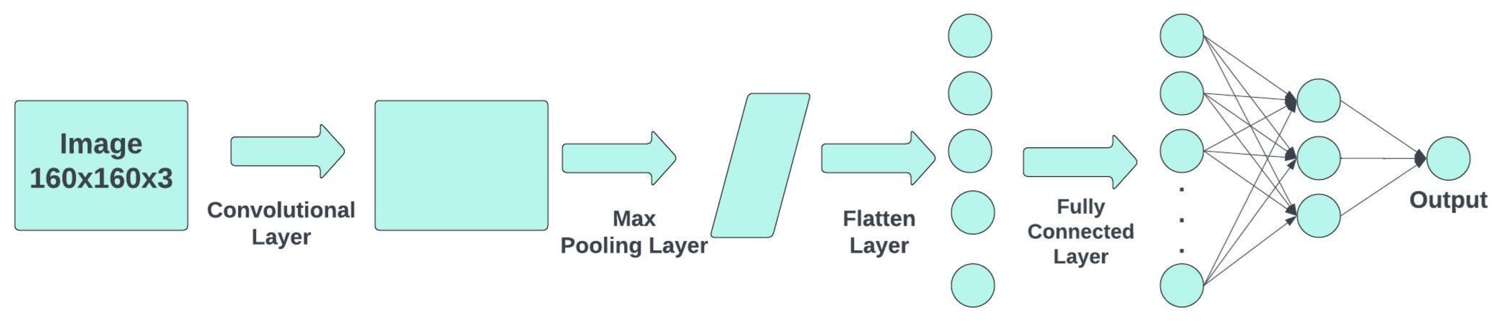
Convolutional neural networks (CNNs) are the basis of DL, as CNNs are made up of deep (multiple-layer) feed-forward artificial neural networks (ANNs) [31]. CNNs have been widely used for image processing tasks such as object detection. As they can learn translationally invariant patterns, they can accurately detect objects wherever they are placed on an image. A CNN is basically composed of 4 types of layers: convolutional, pooling, flattening, and fully connected layers. The convolutional and pooling layers can be used more than once before using the flattening layer. This decreases the computational size and is one of the principles of a CNN. Figure 5 shows a diagram of a convolutional neural network.
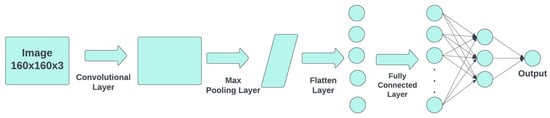
Figure 5.
CNN architecture diagram.
The input of a CNN can be an RGB image, consisting of three channels: red, green, and blue. Each channel has the same image size, which is determined by the number of width pixels and height pixels. The value of each pixel depends on the color depth, and in most cases images have an 8-bit color depth, meaning that the value of each pixel at each channel is in the range of 0 to 255. Using the 3D matrix of the image, a convolutional layer is applied.
The main objective of the convolutional layer is to extract the height-level features of the image. This layer consist of a smaller matrix, which is often called a kernel or filter. Using this filter, a convolutional operation is computed with each channel of the 3D input image. The values of each of the pixels from the filter are called weights.
2.7.2. YOLOv5
YOLOv5 was picked because it is accurate, small, and stable [33]. YOLOv5 builds on YOLOv3, achieving equal detection performance but using only 10% of the space. This makes it efficient and suitable for many uses [34].
YOLOv5 comes in four sizes. YOLOv5s is compact and fast but less accurate. The others (YOLOv5m, YOLOv5l, and YOLOv5x) are slower but more accurate. Figure 5 shows the whole YOLOv5s structure, which has four parts: input, backbone, neck, and prediction.
In the Figure 6, CONVindicates convolution; BN indicates batch normalization; and, finally, CONCAT indicates the feature fusion method of adding up the number of channels.
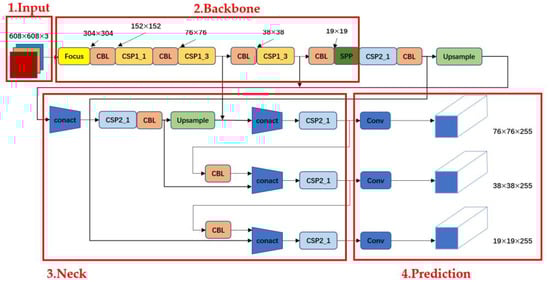
Figure 6.
YOLO architecture diagram.
CBL is a module that encompasses CONV, BN, and Leaky Relu, collectively forming the activation functions. The adaptive anchor is a box predicted from the network’s output.
The predicted and actual boxes are compared to make the network better (backward updates). The best anchor box size is then determined for the dataset. During training, the network dynamically decides the best anchor box for each set [34]. The aspect ratio and bounding box size are set when defining the anchor boxes. Equation (9) shows the formula for finding a bounding box.
The equation uses the following notation: w denotes the width of the bounding box, h represents the height, and s indicates the area of the anchor. By integrating an adaptive anchor during the network’s training process, we improve the model’s accuracy, decrease the computational time, and accelerate the target detection speed. This synergy makes the whole process more efficient and effective [35]. The focus module is utilized in the first layer of the underlying network. An essential step known as slicing is involved. When examining a standard image with dimensions of 3 × 608 × 608 in YOLOv5s, the image is divided into smaller sections, resulting in a 12 × 304 × 304 map. Then, with the help of 32 special filters, as shown in Figure 7, it changes the map to a 32 × 304 × 304 one. This whole process is designed to speed up detection.
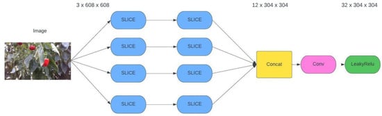
Figure 7.
Focus module diagram.
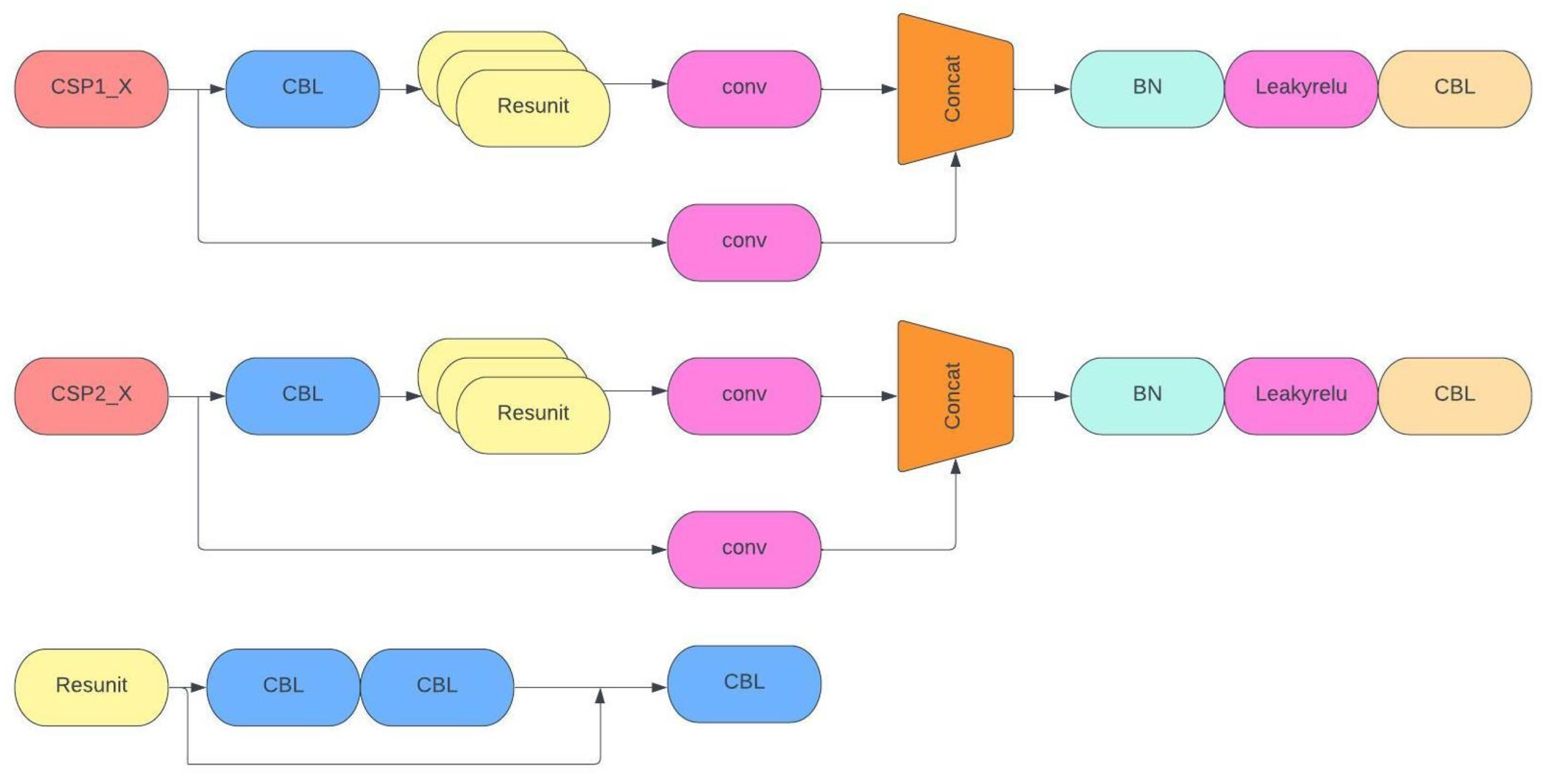
Figure 8 illustrates the structure of the YOLOv5s network, highlighting two significant CSPNet nodes identified as CSP1 and CSP2. CSP1 operates within the backbone, while CSP2 is situated in the neck network. One part focuses on running convolution for more detailed features, while the other combines the processed features. This special design helps the network learn better, maintain accuracy, and use fewer resources. It is also effective for speeding up the process without needing a lot of memory [36]. The Res unit employs ResNet’s special structure to create a deep network.

Figure 8.
CSP diagram.
2.7.3. DeepSORT
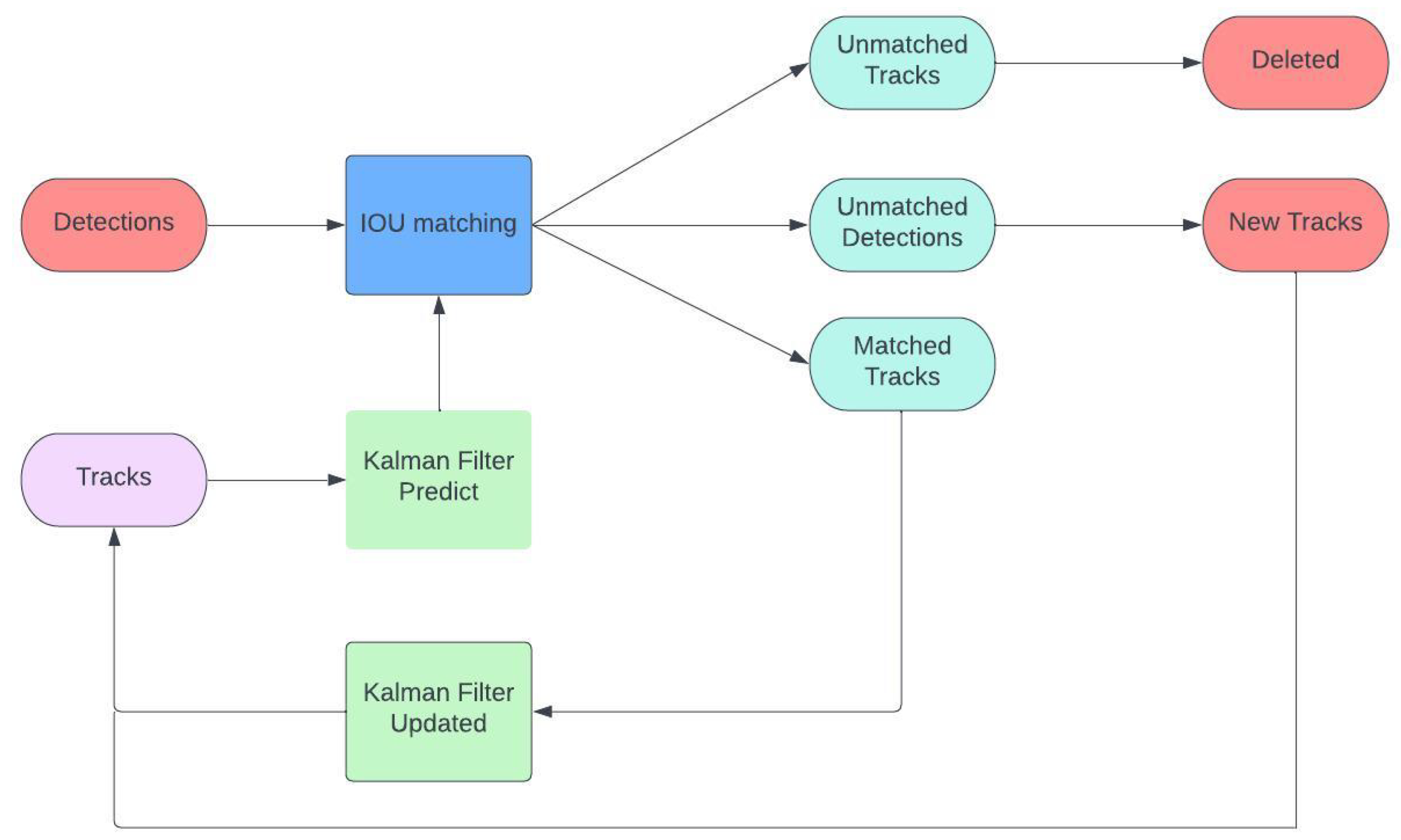
To fix the issues with regular object tracking methods in live videos, DeepSORT uses deep learning. It upgrades the basic but effective search technique known as SORT. SORT struggles when trying to track objects that are too close or hidden. DeepSORT tackles this by connecting identical object detections across frames using deep learning. It checks how similar two detections are, allowing it to follow several objects even when they are close or blocked. DeepSORT is also better at handling changes in how things look and the lighting. The parts of DeepSORT related to estimating and managing tracks work similarly [20]. Figure 9 summarizes how the algorithm works, and Table 2 shows an overview of the DeepSORT structure. We use a wide residual network with specific layers to calculate features and make the system work well with the cosine arrival metric [37].
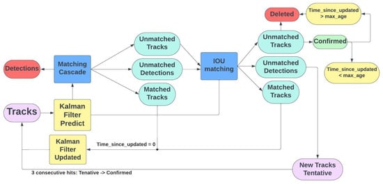
Figure 9.
DeepSORT diagram.
Table 2.
Technical specifications.
The Hungarian technique, similar to SORT, follows a two-step process to match observed bounding boxes with existing tracks. First, we use the DeepSORT method to find suitable tracks based on their movement and appearance. In the second step, we use the same method as SORT to connect new potential tracks with unmatched detections. We calculate the Mahalanobis (squared) distance to consider motion between predicted states and detections. Alongside this distance measure, we also use another metric based on the shortest cosine distance to figure out how separate each measurement’s tracks are in terms of their visual characteristics.
2.7.4. Data Augmentation
In the training of deep CNNs, a common way to improve performance is through data augmentation. This involves artificially expanding the training dataset by making various changes like translations, rotations, flips, cropping, and adding noise, as shown in Figure 10. The two most popular techniques are random flipping and random cropping. Random flipping rotates the input picture horizontally, while random cropping randomly takes out a part of the original image.
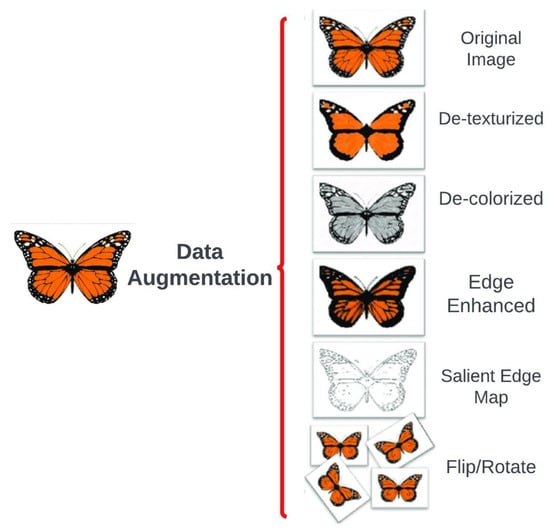
Figure 10.
Data augmentation algorithm diagram.
3. Experimental Setup
3.1. Greenhouse Data Acquisition
The images used for experimentation were captured within the sweet pepper greenhouses at CAETEC (the Experimental Agricultural Field of the Tec de Monterrey) by Luis Enrique Montoya Cavero [38]. We can see an example of the data in Figure 11. The images were acquired with an Intel Real-Sense D435i camera (Intel, 2200 Mission College Blvd, Santa Clara, CA, USA). The Real-Sense camera was configured to produce pixel-aligned RGB and depth images using default settings and a resolution of 1280 × 720 pixels. Figure 12 depicts the technique utilized for taking the photos, with the camera placed perpendicular to the crops at an estimated height of 1.3 m. The horizontal distance between the camera and the crop was approximately 60 cm. These images were taken from 11:00 a.m. to 4:00 p.m. The images were taken at varying distances, angles, and time intervals and under varying lighting situations. At the time of image acquisition, the climate was sunny without clouds. The dataset contained 620 images with different colors of sweet peppers (green, red, yellow, and orange), including heavily overlapping sweet peppers, branch-occluded sweet pepper images, sweet peppers with occlusion and overlaps, leaf-occluded sweet pepper images, and a mix between branch- and leaf-occluded sweet peppers. For other scenarios, generating another dataset with specific conditions was necessary. Additionally, to the base dataset [38], we added one dataset from the Roboflow website [39] to increase the amount of data and obtain better results. Both collections of images were saved in PNG format with identical resolutions:
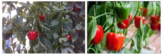
Figure 11.
(Left) CAETEC dataset, (Right) Roboflow dataset.
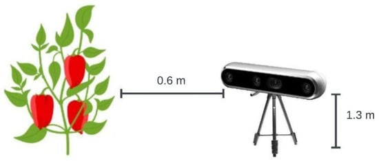
Figure 12.
Image acquisition diagram.
- Training set—70% of the data;
- Validation set—20% of the data;
- Test set—10% of the data.
3.2. Dataset Construction and Health Check
This study included pictures of sweet peppers captured under various natural conditions, avoiding duplication, and resized to a uniform resolution of 640 × 640 pixels to ensure diversity within the image dataset. For training the YOLOv5 model was used the version YOLOv5s, a total of 1863 images were selected. The dataset followed the common practice of allocating 70% of the images for training, 20% for validation, and 10% for testing. Each dataset comprised two main directories: ‘images’ and ‘labels’. After the training and validation, 186 pictures were used to test the model. These images were selected to cover diverse aspects of natural production environments, incorporating variations in daylight illumination spanning the entire harvest period, shadows, overlapping fruits, the presence of leaves and stems from the main crop, and distortions induced by movement. The images used in the experiment had variations in size, visibility, brightness, and the quantity of sweet peppers. These variations represented different ripeness levels and colors. The experiment mainly focused on the most complex color variety of sweet peppers. Therefore, the training and evaluation sets mainly comprised examples of green sweet peppers. This was because they resemble the natural production environment, and the intention was to provide results that closely aligned with the challenges faced in real production scenarios. The aim was to not rely on ideal examples where lighting and other factors were tightly controlled to facilitate analysis. The dataset was a realistic and complex representation of the production environment and encompassed various scenarios. It is essential to mention that the algorithm may not detect sweet peppers correctly in certain situations and in some greenhouses where there may be too little or too much light. Another situation where this could occur is when there are many leaves and the fruit cannot be seen correctly.
In Figure 13a, is a class frequency plot of the dataset. This plot shows how often each class appeared in the dataset. In this case, the immature class appeared the most because there were more images of this class than the others. Having a balanced dataset can improve accuracy. In the same Figure 13b, is a graph that shows the distribution of bounding box labels in relation to normalized height and width space. This graph can help illustrate the variability in box dimensions and identify patterns or anomalies in the distribution. Looking at the graph, we can see that the bounding boxes had different sizes but maintained a pattern. The last plots, in Figure 13c,d, detailed information about the specific position of bounding boxes in relation to image coordinates. These scatter plots represent the specific coordinates of bounding boxes in the dataset. In the context of object detection, bounding boxes are defined by their coordinates, usually the coordinates of the upper-left corner and the lower-right corner. It is worth noting that the dataset in reference [38] was chosen as a base dataset because it has similar characteristics to this experiment, reinforcing its relevance. Another open-source dataset obtained from the Roboflow platform was added to increase the quantity and improve the detection accuracy further [39]. The Roboflow platform is accessible online and free for anyone, making annotating and labeling the experimental dataset for the maturity classification of peppers easy and user-friendly. For more detailed information about the dataset created for this perception system, please refer to the following source: https://github.com/luisviveros/green_sweet_pepper_detection_using_yoloV5_deepsort (accessed on 9 January 2024).
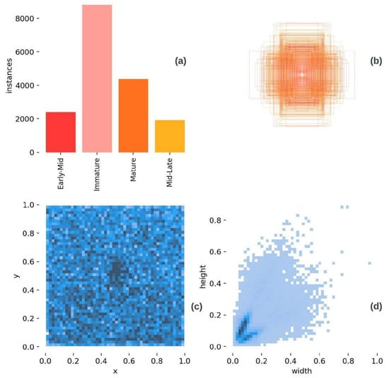
Figure 13.
Label distribution.
3.3. Maturity Classification
This experiment divided pepper maturity into four levels (immature, early-mid, mid-late, mature).
Table 3 shows the maturity levels of the peppers referenced in this study.
Table 3.
Technical specifications.
The cumulative temperature is the accumulated excess or deficit in temperature based on fixed data. It is often closely linked to the color variations in peppers and can be used in crop growth models. With the increasing impact of climate change, cumulative temperature may gain more significance [40]. In a greenhouse, sweet peppers can be harvested from mid-summer until autumn. However, outdoors, plants usually start fruiting later, in August, and finish earlier once temperatures drop in late summer or early autumn. When the fruits become swollen and glossy, it is time to pick them. The majority of peppers ripen from green to red, although some varieties turn yellow, orange, or purple. The fruits become sweeter as they mature, so the peppers can be picked at whichever color and stage of ripeness is preferred.
3.4. YOLOv5 Model Implementation
We utilized YOLOv5s, an open source model package developed by the Ultralytics team, along with Anaconda Environment 23.7.2 running Python 3.11. Our implementation used Keras 2.1.2 and PyTorch 1.8.0, and it was executed on a Dell G7 7790 computer (Dell inc, Round Rock, TX 78682, USA) with a ninth-generation Intel Core i7-9750H processor (Intel, 2200 Mission College Blvd, Santa Clara, CA, USA), an NVIDIA GeForce RTX 2060 Laptop GPU (Nvidia, 2788 San Tomas Expy, Santa Clara, CA, USA), and 16 GB RAM operating at 2666 MHz. The computer ran on a 64-bit Windows 10 operating system (Microsoft Inc., Redmond, WA 98052, Seattle, WA, USA). In order to execute the algorithm, one must have a minimum of an Intel Core i7 processor, 16 GB of RAM, and an NVIDIA RTX 1050 Ti card. If one intends to run the algorithm in real time, a Jetson Nano or Xavier computer that enables the execution of computer vision algorithms is needed. Lastly, a camera with a good resolution is required to ensure that the image is sharp and easily detectable by the model.
During the training process, we employed a graphics processing unit (GPU) and used a batch size of 10 images. To optimize accuracy, we experimented with different learning rates, including 0.001 and 0.0001, and ran the algorithm with varying epochs, namely 80, 200, 250, 300, and 500. We also used a learning momentum of 0.937 and a weight decay of 0.005. We used the COCO (Common Objects in Context) dataset to learn distinctive and standard features as a foundation during the transfer learning process. For data augmentation, we employed techniques such as 90° rotations (clockwise, counter-clockwise, upside down); cropping (ranging from 0% minimum zoom to 20% maximum zoom); blur (up to 2.5 pixels); and noise (up to 5% of pixels). We trained the YOLOv5s model on the “Maturity Peppers in Greenhouse by Objected Detection Image Dataset”, available on the Roboflow platform, which was curated by Luis David Viveros Escamilla in 2023. During the inference process, we set a minimum detection confidence threshold of 85% to ensure that detections with confidence levels below this were disregarded. For a more detailed understanding of our implementation, readers can refer to the original repository of this YOLOv5 model implementation on GitHub (https://github.com/ultralytics/yolov5#pretrained-checkpoints, accessed on 20 March 2022).
3.5. Counting Algorithm
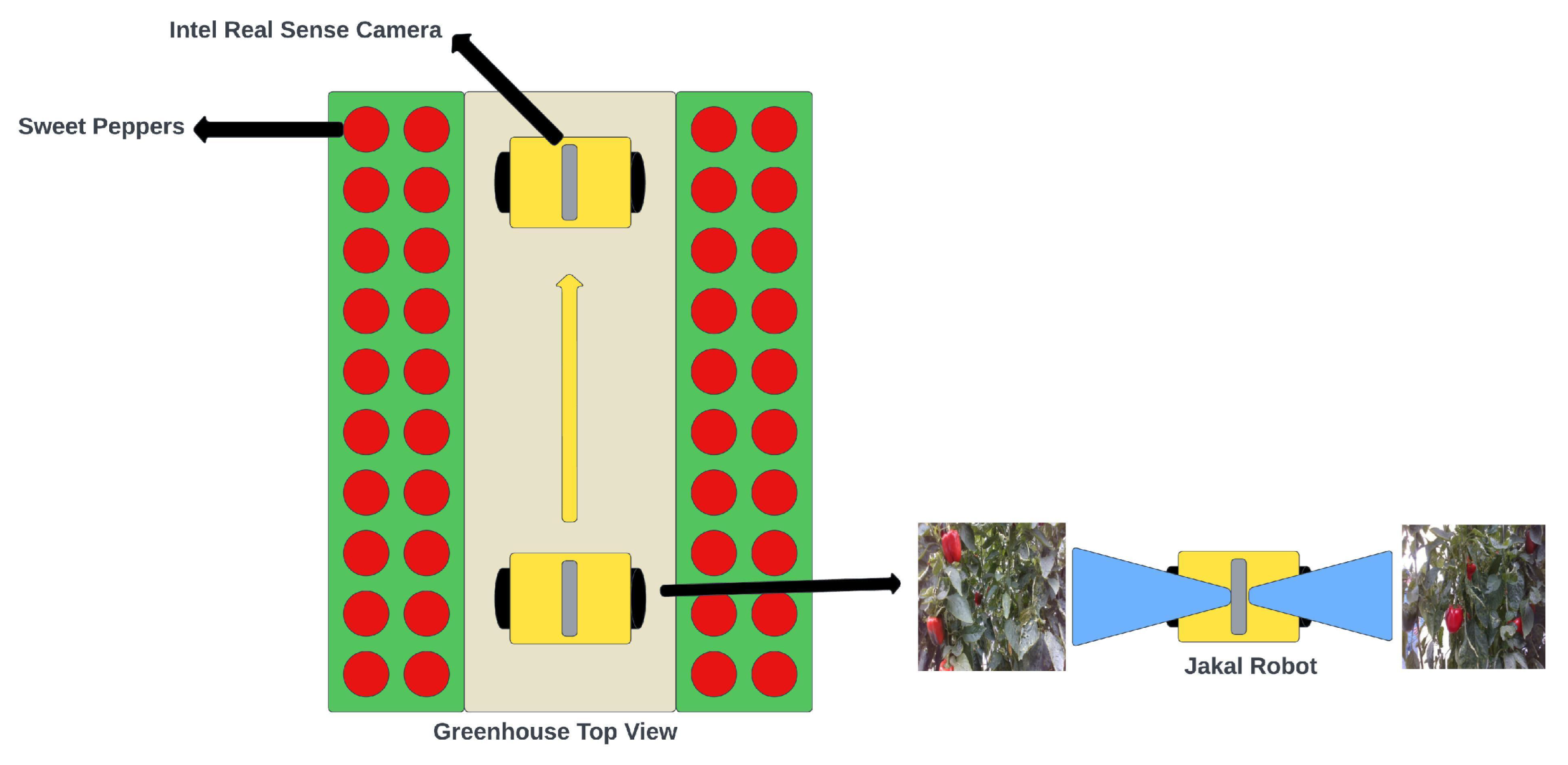
A perception system for sweet peppers in greenhouse agriculture is crucial for estimating harvests. Manual counting, known for its high error rates and time-consuming nature, poses significant challenges. Our study employed the YOLOv5 deep learning model for object detection, combined with the DeepSORT tracking algorithm. This integration within YOLOv5 aimed to improve efficiency and reduce production costs when counting sweet peppers in greenhouse environments. The YOLOv5 deep learning model was trained using an enriched dataset of labeled sweet peppers and the PyTorch library. This trained model detected sweet peppers and their corresponding categories, transmitting the neural network’s weights to the DeepSORT algorithm as shown in Algorithm 1. A deep learning strategy for counting sweet peppers was validated with two simulated environments that were created using Da Vinci Resolve 18.5.1 software to implement the DeepSORT algorithm. Two videos were generated using authentic images captured within the sweet pepper greenhouse at CAETEC. In the video creation process, we utilized 70 photos for each video, with each image possessing a resolution of 640 × 640 pixels, as depicted in Figure 14. These photos were strategically arranged horizontally, creating the visual effect of a robot navigating through the sweet pepper lanes in the greenhouse, as depicted in Figure 15. The initial video sequence, lasting 1 min at a frame rate of five frames per second, was composed of 300 frames and had a total duration of 1.53 min. The subsequent video, also lasting 1 min at five frames per second, comprised 300 frames and extended over 2.17 min. In total, the two videos incorporated 70 images, providing a comprehensive representation of the sweet pepper greenhouse scenario. For more detailed information, please refer to the following GitHub repository (Luis David Viveros Escamilla, 2023a): https://github.com/luisviveros/green_sweet_pepper_detection_using_yoloV5_deepsort.git (accessed on 9 January 2024).
| Algorithm 1: Algorithm for Inspection and Counting Utilizing Distance-Based Filtering |
Step 1: Specify DeepSORT configurations as cfg Step 2: Start DeepSORT (DeepSORT algorithm, cfg) Step 3: Set up the device (GPU) Step 4: Detect Multi Backend (v5 model, device = GPU, dnn = opt.dnn) video_path = simulation_environments_video_file detections = model (video_path, increase = opt. increase, visual = visualize) #Detect processes for i, detection in enumerate (detections): #Perception per image #Find detections confidences, classes, boxes = find (detection) #Transfer the detection to DeepSORT deep_sort_outputs = deep-sort update (boxes.cpu (), confidences.cpu (), classes.cpu (), img) #For visualization, make bounding boxes. size_filter = (max_height, max_width) if leng(deep_sort_outputs) > 0: for j, (output, confidence) in enumerate (zip (deep_sort_outputs, confidences)): category = int(classes) #Integer class y_coord, x_coord= find_y_x (output) #Apply size filter if y_coord * x_coord > size_filter: # Classify and process based on class if category == 0: #class 0 is immature elif category == 1: #class 1 is early-mid elif category == 2: #class 2 is mid-late elif category == 3: #class 3 is mature #Stream Results #Save Results (image with detections) |
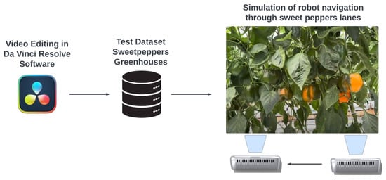
Figure 14.
Simulation environment video creation.
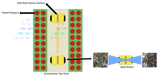
Figure 15.
Equipment setup.
4. Results and Discussions
During the experiment, the original image had a resolution of 1280 × 720 pixels. To improve the speed of processing, the input for the algorithm was preprocessed and adjusted to 640 × 640 pixels. For training the detection model, 1863 images were chosen featuring common sweet pepper varieties such as green, red, yellow, and orange. These images were divided into 70% for the training dataset, 20% for the validation dataset, and 10% for the test dataset. The detection model was configured to have four output categories: mature, immature, early-mid, and mid-late. In order to evaluate the performance, stability, and reliability of the trained model, 186 images of sweet peppers were chosen for model evaluation. The objective was to detect, classify, and annotate all sweet pepper fruits and peduncles in the images with category scores and bounding boxes. For the tracking model, two videos were used for training and testing, with MOTA (Multiple-Object Tracking Algorithm) metrics employed to evaluate the results, offering insight into the effectiveness of our detection and tracking methods.
4.1. Best Fit Epoch Performance Comparison
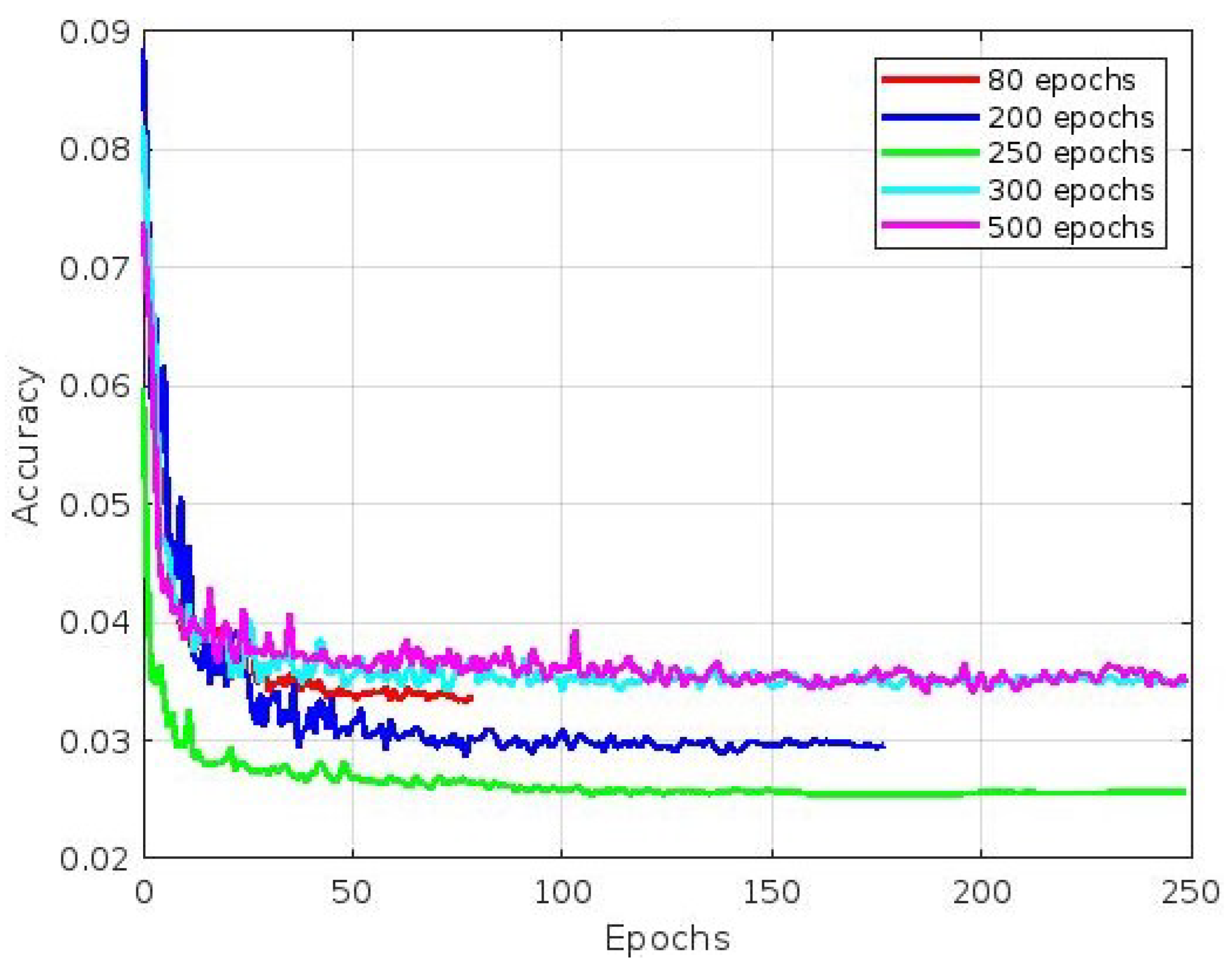
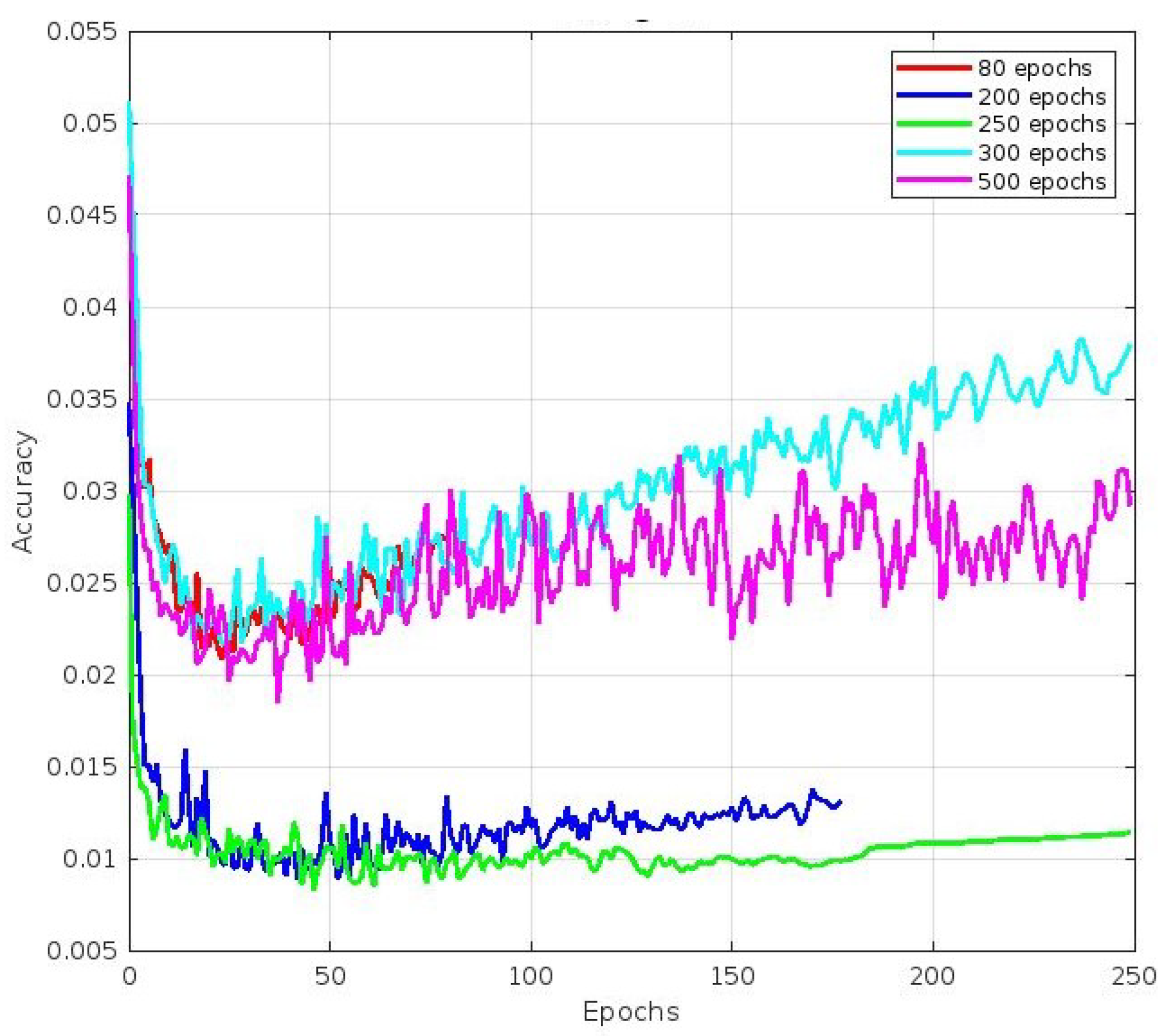
Our experiment collected a dataset of 1863 images featuring different sweet pepper varieties, such as green, red, yellow, and orange. To evaluate the performance, stability, and reliability of our trained model, we set aside 186 images of sweet peppers for model evaluation. We aimed to detect, classify, and annotate all sweet pepper fruits in the images, assigning appropriate category scores and bounding boxes as necessary. We trained the YOLOv5 model with different numbers of epochs, namely 80, 200, 250, 300, and 500, to achieve the best precision. We also used early stopping techniques to prevent overfitting, which allowed us to stop the training process at any point to avoid wasting time. After each epoch, we generated a file containing the synaptic weight values up to that point, enabling us to access the synaptic values of the model at any given time. Additionally, we recorded the training and validation loss values for each epoch using a tensorboard. The following text summarizes the results of an experiment. Figure 16 shows the convergence of mAP curve images, where the best mAP value was achieved after 250 epochs, followed by 200 epochs. Figure 17, Figure 18 and Figure 19 refer to different components of the loss function used during training. These components helped the model learn to detect and classify objects within an image. Figure 17 depicts the accuracy of the predicted bounding box coordinates (x, y, w, h) compared to the ground-truth bounding box coordinates. This metric is typically calculated using a loss function like the Mean Squared Error (MSE) or a variant. The plot shows that the best accuracy value was achieved after 250 epochs, followed by 200 epochs. Figure 18 depicts how well the model detected objects within the image. It compares the predicted objectness score (obj) with the ground-truth label (0 or 1), indicating whether an object was present in a particular grid cell or anchor box. The cross-entropy loss or a variant is commonly used to compute this part of the loss. The plot shows that the best accuracy value was achieved after 250 epochs, followed by 500 epochs. Finally, Figure 19 is related to how well the model classified detected objects into specific classes. It compares the predicted class probabilities (cls) with the ground-truth class labels encoded via one-hot encoding. Similar to object detection loss, the cross-entropy loss or its variations are often used to compute this part of the loss. The plot shows that the best accuracy value was achieved after 250 epochs, followed by 200 epochs.
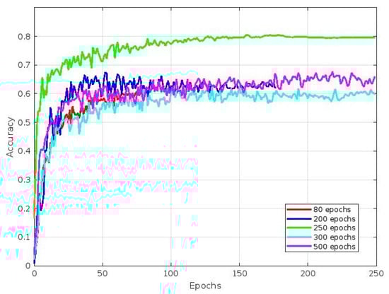
Figure 16.
Mean average precision (mAP@0.5).
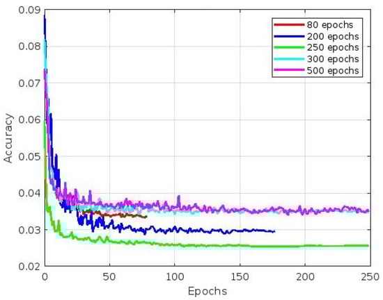
Figure 17.
Bounding box coordinates loss.
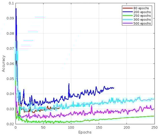
Figure 18.
Object detection loss.
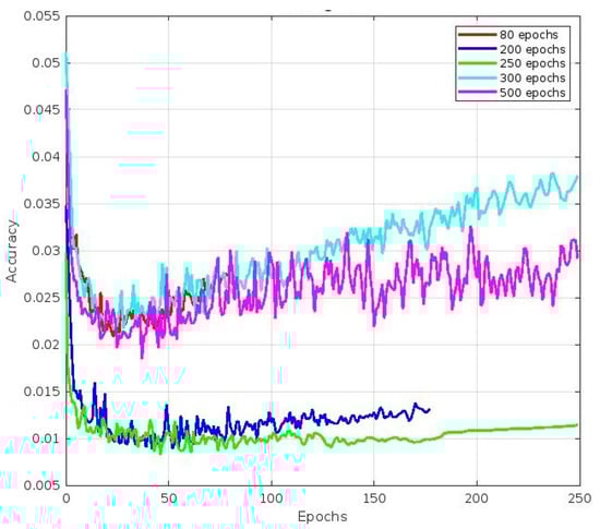
Figure 19.
Classification loss.
4.2. Maturity Recognition Results
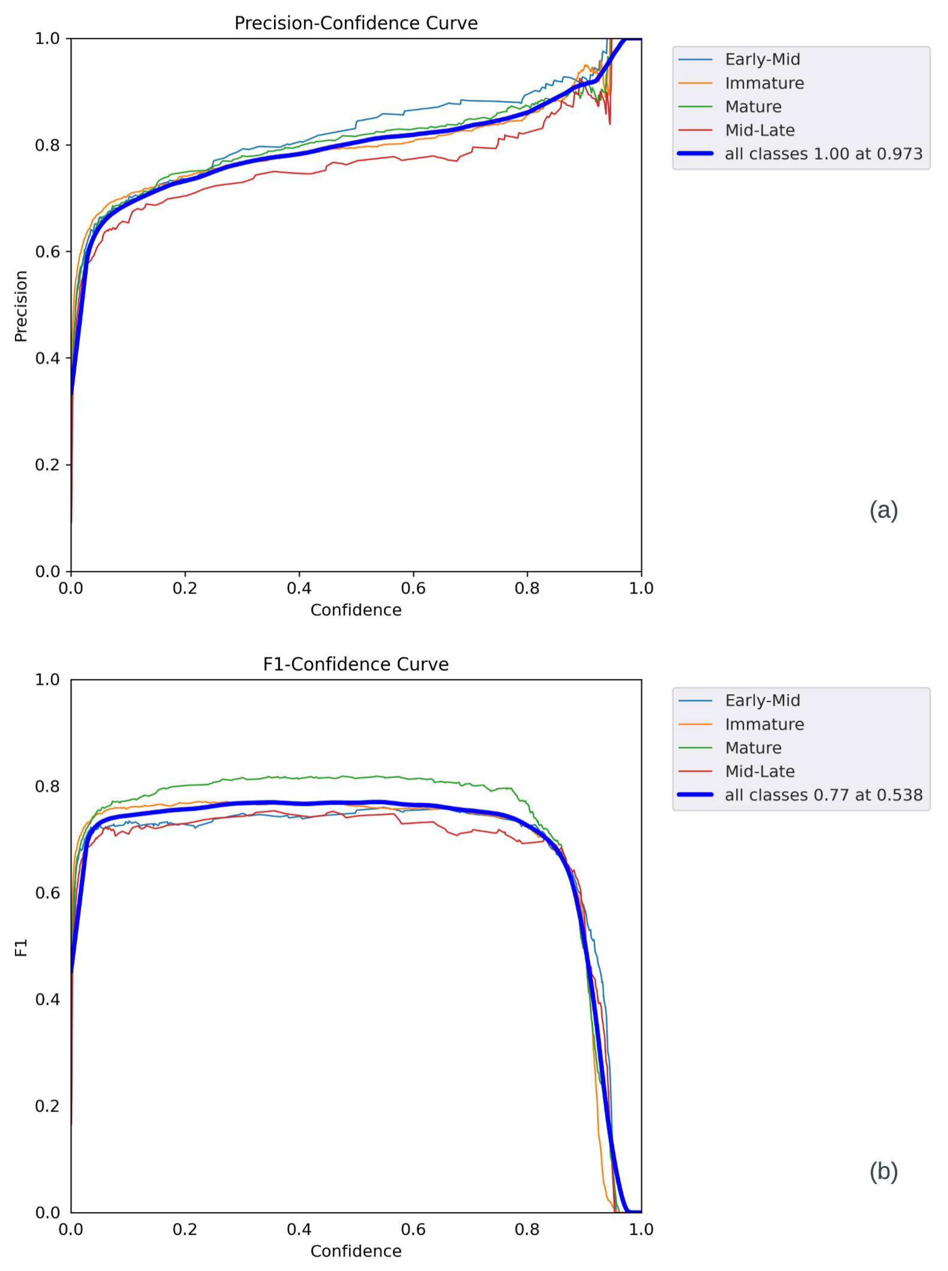
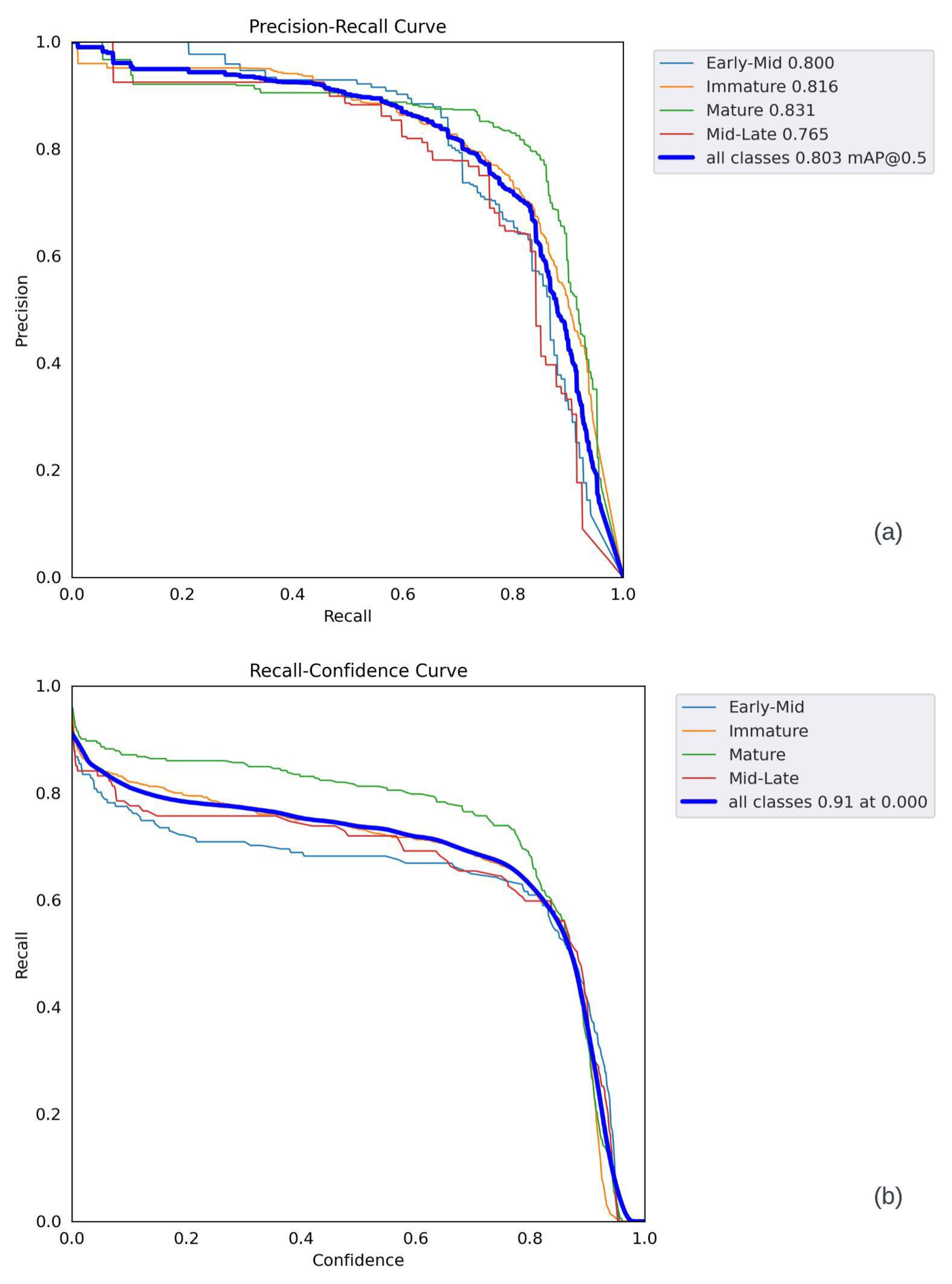
The following observations can be made from the graphs presented in Figure 20 and Figure 21. In Figure 20a, the confidence increases as the F1 level reaches 1. The best F1 score was 0.77, with a confidence level of 0.538. The overall shape of the curve suggests that the model was able to achieve good F1 scores (above 0.5) for objects with medium confidence scores (around 0.5). In Figure 20b, the precision increases almost linearly as the confidence level reaches 1. The best precision occurred at a confidence level of 0.973, indicating a relatively high number of correct positive values in all categories. In Figure 21a, the recall values provide valuable insights into the prediction performance. It can be observed that the recall values gradually decreased as the confidence level increased. This trend was due to the increased impact of the false-negative detection of sweet peppers on prediction accuracy. Furthermore, the PR curve shows that various thresholds impacted different classes, and the Mid-Late class displayed inconsistent behavior due to the lower number of annotations. The individual F1 scores for the mature, immature, early-mid, and mid-late categories were 0.82, 0.76, 0.69, and 0.68, respectively, with a confidence level of 0.538. At the same confidence level, the collective F1 score for all models rapidly increased, reaching its peak at 0.77. Nevertheless, once the confidence level surpassed 0.8, the F1 score gradually declined. As shown in Figure 21b, the most accurate predictions occurred within the confidence range of 0.5 to 0.8. Due to the larger number of annotations for the sweet pepper category, its F1 score rapidly increased. Using the optimal sweet pepper detection model, the subsequent prediction was generated and evaluated across various images, illustrated in batches in Figure 22.
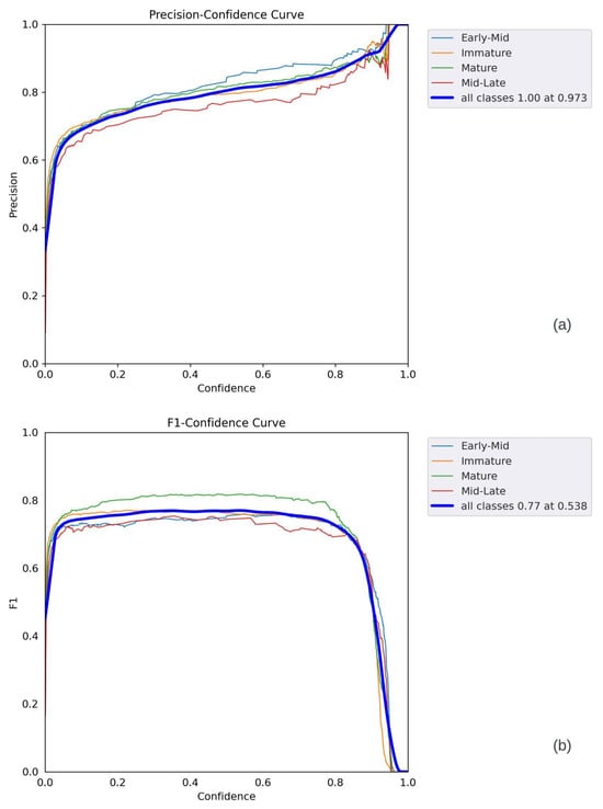
Figure 20.
YOLOv5 performance parameters: (a) F1 curve, (b) P curve.
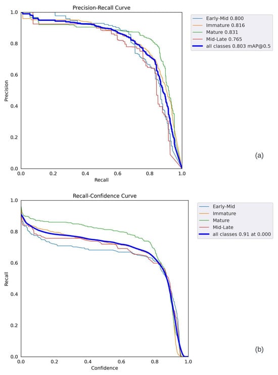
Figure 21.
YOLOv5 performance parameters: (a) R curve, (b) P–R curve.
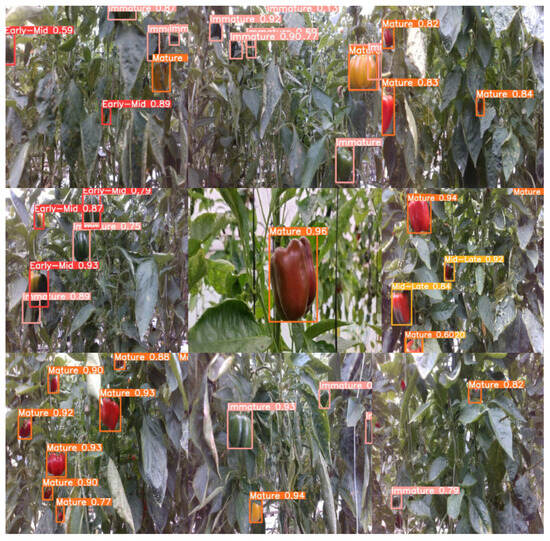
Figure 22.
Validation results.
Figure 23 shows this section’s confusion matrix chart. The chart displays how well the model performed in recognizing different stages of maturity. The model’s ability to recall items at the early-mid, immature, mature, and mid-late stages was 69%, 79%, 86%, and 71%, respectively. However, there were still some areas for improvement in the model’s recognition capabilities. For instance, around 7% of mid-late-stage sweet peppers were incorrectly identified as early-mid-stage, and 2% were misclassified as immature. Similarly, roughly 1% of mature-stage sweet peppers were mistakenly labeled as immature, and about 2% were categorized as mid-late-stage. Additionally, approximately 5% of early-mid-stage peppers were incorrectly identified as mature-stage. The confusion matrix helped us to identify areas where the model could have performed better. It was observed that less than 2% of all detections were incorrect. The last column in the matrix shows where the model falsely detected small, unlabeled sweet peppers in the dataset. The results indicate that the best weights were obtained at epoch 250 with a 0.803 mAP 0.5. The training results are presented in Table 4.
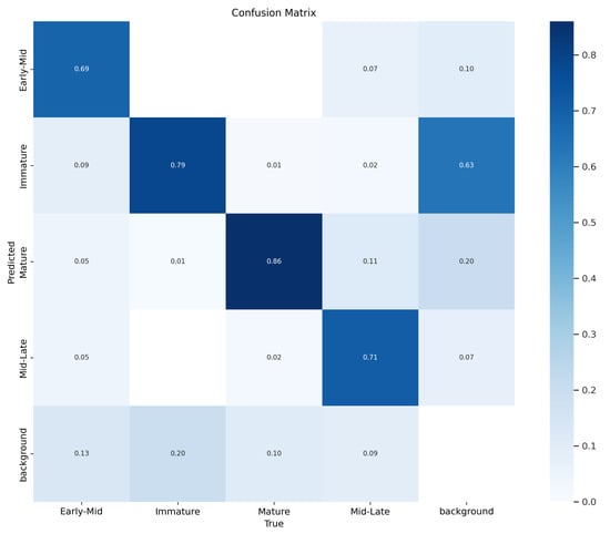
Figure 23.
Confusion matrix.
Table 4.
Best mAP@0.5 and mAP@0.95 performance parameter results.
As per the details given in Table 4, it can be observed that the early-mid class had a better prediction accuracy than the other classes. This was because the early-mid class had more training samples, and their color features were distinct. However, the immature class had a lower prediction accuracy because most surveyed areas in the greenhouse environment had green leaves. The mid-late class had the lowest prediction accuracy due to the limited number of samples. To evaluate the model’s performance, we considered the best precision, recall, and F1 scores in relation to the confidence level plots and PR curves. Figure 16, Figure 17, Figure 18 and Figure 19 provide a clear picture of the same.
4.3. DeepSORT Results
After training the model, we used the DeepSORT algorithm to track the sweet peppers that we identified and determine their positions. Object detection algorithms such as YOLOv5 use mean average precision () to evaluate their object detection performance. However, since our main goal was to monitor the movement of vehicles within a frame, it was important to verify our findings using an object tracking algorithm. We used MOTA (Multiple-Object Tracking Algorithm) metrics to assess the performance of our detection and tracking methods. We first needed to define , , , and . Detailed explanations of these definitions can be found in Table 5. We used Equation 10 to calculate the , where represents the absence of a match with the real object in the ground-truth data. This could occur when the sweet pepper was too distant from the camera or due to bad weather or lighting. refers to instances where the algorithm detected something, but there was no real object in the ground-truth data. We had one case of an , where the algorithm mistook a reflection of a mid-late sweet pepper for an immature pepper. occurred when the algorithm mistakenly switched the identification of tracked fruits. Lastly, denotes all real ground-truth objects.
Table 5.
Definition and description of IDS, GT, FP, and FN.
Figure 24 illustrates samples of sweet pepper detection and tracking in a greenhouse environment using YOLOv5 with an object tracking algorithm. Each video contained around 70 images of 640 × 640 size from the greenhouse of CAETEC. According to Table 6, the performance of YOLOv5 with DeepSORT was very good, presenting high accuracy in both simulation environments with an accuracy difference between the two of only 0.01. The algorithm often altered vehicle IDs, causing inaccuracies in tracking that impacted the overall performance. This occurred because, in some images, the occlusion by leaves prevented the complete detection of the bell pepper, creating a misleading impression. Additionally, variations in lighting conditions could also impact the accuracy of detection. Sometimes, the image was too bright or too dim, leading to distortion in the color of the fruit and the incorrect detection of the bell pepper as mature when it was actually in an intermediate stage of ripeness. However, these issues had a minimal impact on the DeepSORT algorithm, as its primary goal was to count the peppers, regardless of potential inaccuracies in determining their maturity level. What mattered most to the algorithm was successful detection and subsequent tracking. On a different note, one of the parameters that could directly influence the algorithm was the presence of false negatives (FNs) and false positives (FPs). As shown in Table 6, we had a deficient number of FPs, indicating a high level of accuracy. This was achieved by configuring the to be as precise as possible, preventing overdetection. FPs had a more pronounced impact on our results, affecting our precision. This was mainly due to situations where leaves obscured the sweet peppers, making it challenging for the algorithm to detect them, as only a small portion was visible. This situation could also affect the accuracy of counting. Comparatively, a human harvester may encounter similar challenges, as the human eye is not infallible and may only sometimes identify 100% of the fruits due to the same visual obstructions.
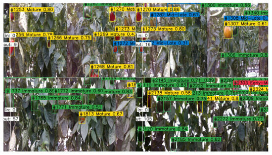
Figure 24.
DeepSORT validation results.
Table 6.
Performance comparison of the two simulation environments.
Our study comprised a comprehensive dataset of 1863 images featuring sweet peppers. We divided this dataset into three subsets, training, validation, and evaluation, which were essential in achieving our success. We trained our model at different intervals (80, 200, 250, 300, and 500 epochs) and utilized early stopping techniques to prevent overfitting. It was discovered that having a balanced dataset was critical for precise detection. If one category had more images than another, it could reduce the model’s accuracy. Therefore, it was important to have a balanced dataset from the beginning of the project. During the training process, we closely monitored various aspects of the loss function to ensure that the model’s bounding box location prediction, object detection, and classification ability improved as training progressed. Our results showed that the model achieved its highest accuracy at epoch 250, followed closely by epoch 200. We also evaluated the model’s accuracy at different confidence levels and found that the best precision was achieved at a confidence level of 0.973. This means that the model correctly identified many positive cases across all categories. However, we found that the recall values gradually decreased as the confidence level increased, mainly because false-negative detections significantly impacted the accuracy, particularly with sweet peppers.
We calculated the F1 scores for different classes and collective F1 scores at various confidence levels. The highest collective F1 score of 0.77 was observed within the confidence range of 0.5 to 0.8, indicating that this range produced the most accurate predictions. Despite the model’s overall high accuracy, we faced some challenges. One of them was the misclassification of different maturity stages for sweet peppers. For example, the model sometimes could not distinguish mid-late-stage sweet peppers from early-mid-stage or immature ones. It also occasionally misidentified mature-stage sweet peppers as immature or mid-late-stage sweet peppers. Our findings highlighted the significance of the confidence level in recognizing objects, and we found that the most accurate predictions were made within the confidence range of 0.5 to 0.8.
We found that beyond a confidence level of 0.8, the F1 score gradually decreased. Our study involved using the DeepSORT algorithm to track sweet peppers in a greenhouse, and we obtained high accuracy results with minimal differences between different simulation conditions. However, we identified some challenges related to leaves obstructing the peppers and changes in lighting conditions, which affected the detection accuracy. Nevertheless, the DeepSORT algorithm was effective in counting peppers, even when inaccuracies in determining their maturity level occurred. Our research successfully developed and evaluated a system for detecting and tracking sweet peppers in a greenhouse. The YOLOv5 model and the DeepSORT algorithm performed well, showing high precision and accuracy in recognizing and tracking sweet peppers. Despite some challenges, our study provides valuable insights for creating automated systems to monitor and harvest crops in the agriculture industry:
- Importance of Dataset Balance:Our study underscored the critical significance of maintaining a balanced dataset from the project’s inception. Ensuring an even distribution of images across different categories is essential for preventing accuracy reduction in the model.
- Optimal Training Epochs: Through meticulous training with various numbers of epochs, we identified the optimal points for model performance, emphasizing the significance of balancing training time to prevent overfitting and achieve stability.
- Challenges in Maturity Stage Classification: Our study revealed challenges in accurately classifying sweet peppers’ maturity stages. Misclassifications, such as confusing mid-late-stage sweet peppers with early-mid or immature ones, provided insights into areas for further refinement.
- Impact of Confidence Levels on Recall: As confidence levels increased, recall values gradually decreased, particularly with sweet peppers. Understanding this impact is crucial for optimizing model performance, especially in scenarios where minimizing false negatives is paramount.
- F1 Score Optimization: The collective F1 score peaked at 0.77, within the confidence range of 0.5 to 0.8. This indicates the importance of selecting an appropriate confidence threshold for achieving the most accurate predictions.
- Applicability of DeepSORT Algorithm: The successful application of the DeepSORT algorithm for tracking sweet peppers in a greenhouse environment showcased its robustness and effectiveness, even in the face of challenges such as occlusions and changing lighting conditions.
- Consideration of Environmental Factors: Our research highlighted the impact of environmental factors on detection accuracy, such as leaves obstructing peppers and variations in lighting conditions. Understanding and accounting for these factors are crucial for developing resilient, automated systems.
Two articles on the state of the art share some similarities to our work but have substantial differences. Dassaef et al. [15] used a Mask R-CNN to detect the fruit and the peduncle of sweet peppers in greenhouse environments, achieving an mAP of 72.64%, while we used YOLOv5 for detecting the maturity level of sweet peppers, obtaining an mAP of 80%. In addition, we used DeepSORT for counting the number of sweet peppers per lane in a greenhouse. On the other hand, Zhang et al. [24] used Orange YOLO to detect oranges in trees and employed Orange Sort, a modified version of SORT for counting. Nevertheless, our application is specific to sweet peppers and has the capacity to measure the level of maturity.
Some of the challenges that affect the performance of this method include meeting the minimum computer and camera system specifications mentioned in Section 3, ensuring adequate lighting conditions, and generating a robust dataset. Additionally, for different greenhouses, it is necessary to generate a specific dataset and adapt the system to the new conditions of the scenario. It is recommended to provide good lighting conditions and a dataset that considers all the specific conditions of the application.
5. Conclusions
In our study, we developed a robust system that can detect and track sweet peppers in greenhouse environments. We utilized the YOLOv5 model for object detection and the DeepSORT algorithm for tracking, which provided us with promising results in recognizing sweet pepper maturity levels and counting fruits efficiently. Our research made noteworthy contributions to the field of agricultural automation. We created a comprehensive dataset of 1863 images that encompassed different varieties and maturity stages of sweet peppers, which was pivotal to the success of our study. We split this dataset into training, validation, and evaluation subsets, which allowed us to optimize the performance of our model. We found that a balanced dataset is essential for accurate detection, and imbalanced datasets can lead to reduced model accuracy. During the training process, we discovered that our model’s ability to predict bounding box locations, detect objects, and classify them accurately improved over time, with the most significant gains occurring around epoch 250. We also emphasized the significance of confidence levels in object recognition. While we achieved high precision at a confidence level of 0.973, higher confidence levels led to a gradual decrease in recall, primarily due to false-negative detections. The most accurate predictions were consistently within the confidence range of 0.5 to 0.8. In addition to object detection, we successfully applied the DeepSORT algorithm for tracking sweet peppers. This approach demonstrated high accuracy, with minimal variations between different simulation conditions. Despite challenges related to occlusions and changing lighting conditions, the DeepSORT algorithm effectively counted peppers, even when inaccuracies in determining their maturity level occurred. Our research offers valuable insights into the development of automated systems for crop monitoring and harvesting in agricultural settings. The combination of YOLOv5 and DeepSORT presents a promising solution for enhancing the efficiency and accuracy of farming processes, particularly in the context of sweet pepper production. The dataset that was created to recognize sweet peppers could only identify them in certain scenarios. Although it could recognize them in the majority of scenarios, it may not be able to identify them in all cases. The cases where this could be more difficult occur in greenhouses with high or low light levels or in situations where the leaves are on top of the fruit and cover it almost completely. The best way to overcome this limitation is to gradually enrich the dataset by adding more images for different situations when the algorithm does not detect the fruit. This will make the algorithm more robust and versatile. Additionally, it is important to expand the dataset to include other fruits in greenhouses in order to improve the dataset’s ability to detect fruits beyond sweet peppers.
In conclusion, our study advances the state of the art in sweet pepper maturity recognition and fruit counting, providing a foundation for developing more sophisticated automation systems in greenhouse agriculture. The results and insights obtained from this research hold the potential to revolutionize crop management and contribute to more sustainable and productive farming practices.
In future work, due to the results obtained, there are several promising avenues for future research and development. These include the following:
- Expanding the dataset with more diverse environmental conditions and sweet pepper varieties to further improve model robustness.
- Fine-tuning the YOLOv5 model with larger datasets and experimenting with different architectural variations related to object detection such as Mask R-CNN in order to boost accuracy.
- Extending the system’s capabilities to recognize and count multiple fruit and vegetable species, providing a more comprehensive solution for greenhouse agriculture.
- Adapting the system for real-time application, enabling instantaneous decision making during the harvesting process and thus optimizing resource allocation and efficiency.
- Exploring the integration of robotic arms or autonomous vehicles for the automated harvesting of ripe sweet peppers, taking the system from a monitoring solution to a fully automated harvesting system.
- Investigating the implementation of edge computing solutions to minimize the dependency on cloud-based processing and ensure low data analysis and decision-making latency.
- Creating predictive models that use data from monitoring sweet pepper crops to estimate the best times for harvest and crop yield, helping with resource planning and sustainability.
- Designing user-friendly interfaces for greenhouse operators to configure and customize the system, promoting ease of use and adaptability across various greenhouse setups.
Author Contributions
Conceptualization, L.D.V.E., A.G.-E. and J.A.E.C.; methodology, L.D.V.E., A.G.-E. and J.A.E.C.; software, L.D.V.E. and J.A.C.-C.; validation, L.D.V.E.; formal analysis, L.D.V.E., A.G.-E. and J.A.E.C.; investigation, L.D.V.E.; resources, J.A.E.C.; data curation, L.D.V.E.; writing—original draft preparation, L.D.V.E.; writing—review and editing, L.D.V.E., A.G.-E., J.A.E.C. and J.A.C.-C.; visualization, L.D.V.E.; supervision, A.G.-E. and J.A.E.C.; project administration, J.A.E.C. and A.G.-E.; funding acquisition, A.G.-E. All authors have read and agreed to the published version of the manuscript.
Funding
This research received no external funding.
Institutional Review Board Statement
Not applicable.
Data Availability Statement
The data that support the findings of this study are available on GitHub via [41].
Acknowledgments
We acknowledge CONACyT for supporting the postgraduate studies of the first author.
Conflicts of Interest
The authors declare no conflicts of interest.
References
- Osman, Y.; Dennis, R.; Elgazzar, K. Yield estimation and visualization solution for precision agriculture. Sensors 2021, 21, 6657. [Google Scholar] [CrossRef] [PubMed]
- Syal, A.; Garg, D.; Sharma, S. A Survey of Computer Vision Methods for Counting Fruits and Yield Prediction. Int. J. Comput. Sci. Eng. 2013, 2, 346–350. [Google Scholar]
- Mavridou, E.; Vrochidou, E.; Papakostas, G.A.; Pachidis, T.; Kaburlasos, V.G. Machine vision systems in precision agriculture for crop farming. J. Imaging 2019, 5, 8. [Google Scholar] [CrossRef]
- Mekhalfi, M.L.; Nicolò, C.; Ianniello, I.; Calamita, F.; Goller, R.; Barazzuol, M.; Melgani, F. Vision system for automatic on-tree kiwifruit counting and yield estimation. Sensors 2020, 20, 4214. [Google Scholar] [CrossRef] [PubMed]
- Lomte, V.M.; Sabale, S.; Shirgaonkar, R.; Nagathan, P.; Pawar, P. Fruit Counting and Maturity Detection using Image Processing: A Survey. Int. J. Res. Eng. Sci. Manag. 2019, 2, 809–812. [Google Scholar]
- Cong, P.; Li, S.; Zhou, J.; Lv, K.; Feng, H. Research on Instance Segmentation Algorithm of Greenhouse Sweet Pepper Detection Based on Improved Mask RCNN. Agronomy 2023, 13, 196. [Google Scholar] [CrossRef]
- Zhao, Y.; Gong, L.; Zhou, B.; Huang, Y.; Liu, C. Detecting tomatoes in greenhouse scenes by combining AdaBoost classifier and colour analysis. Biosyst. Eng. 2016, 148, 127–137. [Google Scholar] [CrossRef]
- Liu, G.; Mao, S.; Kim, J.H. A Mature-Tomato Detection Algorithm Using Machine Learning and Color Analysis. Sensors 2019, 19, 23. [Google Scholar] [CrossRef]
- Liu, L.; Li, Z.; Lan, Y.; Shi, Y.; Cui, Y. Design of a tomato classifier based on machine vision. PLoS ONE 2019, 14, e0219803. [Google Scholar] [CrossRef]
- Alajrami, M.A.; Abu-Naser, S.S. Type of Tomato Classification Using Deep Learning. Int. J. Acad. Pedagog. Res. 2019, 3, 21–25. [Google Scholar]
- Long, J.; Zhao, C.; Lin, S.; Guo, W.; Wen, C.; Zhang, Y. Segmentation method of the tomato fruits with different maturities under greenhouse environment based on improved Mask R-CNN. Nongye Gongcheng Xuebao/Trans. Chin. Soc. Agric. Eng. 2021, 37, 100–108. [Google Scholar] [CrossRef]
- Su, F.; Zhao, Y.; Wang, G.; Liu, P.; Yan, Y.; Zu, L. Tomato Maturity Classification Based on SE-YOLOv3-MobileNetV1 Network under Nature Greenhouse Environment. Agronomy 2022, 12, 1638. [Google Scholar] [CrossRef]
- Moreira, G.; Magalhães, S.A.; Pinho, T.; Dos Santos, F.N.; Cunha, M. Benchmark of Deep Learning and a Proposed HSV Colour Space Models for the Detection and Classification of Greenhouse Tomato. Agronomy 2022, 12, 356. [Google Scholar] [CrossRef]
- Moon, T.; Park, J.; Son, J.E. Prediction of the fruit development stage of sweet pepper (Capsicum annum var. annuum) by an ensemble model of convolutional and multilayer perceptron. Biosyst. Eng. 2021, 210, 171–180. [Google Scholar] [CrossRef]
- López-Barrios, J.D.; Escobedo Cabello, J.A.; Gómez-Espinosa, A.; Montoya-Cavero, L.E. Green Sweet Pepper Fruit and Peduncle Detection Using Mask R-CNN in Greenhouses. Appl. Sci. 2023, 13, 6296. [Google Scholar] [CrossRef]
- Seo, D.; Cho, B.H.; Kim, K. Development of monitoring robot system for tomato fruits in hydroponic greenhouses. Agronomy 2021, 11, 2211. [Google Scholar] [CrossRef]
- Gomes, J.F.S.; Leta, F.R. Applications of computer vision techniques in the agriculture and food industry: A review. Eur. Food Res. Technol. 2012, 235, 989–1000. [Google Scholar] [CrossRef]
- Halstead, M.; Ahmadi, A.; Smitt, C.; Schmittmann, O.; McCool, C. Crop Agnostic Monitoring Driven by Deep Learning. Front. Plant Sci. 2021, 12, 786702. [Google Scholar] [CrossRef] [PubMed]
- Rapado-Rincón, D.; van Henten, E.J.; Kootstra, G. Development and evaluation of automated localisation and reconstruction of all fruits on tomato plants in a greenhouse based on multi-view perception and 3D multi-object tracking. Biosyst. Eng. 2023, 231, 78–91. [Google Scholar] [CrossRef]
- Wojke, N.; Bewley, A.; Paulus, D. Simple online and realtime tracking with a deep association metric. In Proceedings of the 2017 IEEE International Conference on Image Processing (ICIP), Beijing, China, 17–20 September 2017; pp. 3645–3649. [Google Scholar] [CrossRef]
- Kirk, R.; Mangan, M.; Cielniak, G. Robust Counting of Soft Fruit through Occlusions with Re-Identification; Springer: Berlin/Heidelberg, Germany, 2021; pp. 211–222. [Google Scholar] [CrossRef]
- Villacrés, J.; Viscaino, M.; Delpiano, J.; Vougioukas, S.; Auat Cheein, F. Apple orchard production estimation using deep learning strategies: A comparison of tracking-by-detection algorithms. Comput. Electron. Agric. 2023, 204, 107513. [Google Scholar] [CrossRef]
- Egi, Y.; Hajyzadeh, M.; Eyceyurt, E. Drone-Computer Communication Based Tomato Generative Organ Counting Model Using YOLO V5 and Deep-Sort. Agriculture 2022, 12, 1290. [Google Scholar] [CrossRef]
- Zhang, W.; Wang, J.; Liu, Y.; Chen, K.; Li, H.; Duan, Y.; Wu, W.; Shi, Y.; Guo, W. Deep-learning-based in-field citrus fruit detection and tracking. Hortic. Res. 2022, 9, uhac003. [Google Scholar] [CrossRef]
- van Herck, L.; Kurtser, P.; Wittemans, L.; Edan, Y. Crop design for improved robotic harvesting: A case study of sweet pepper harvesting. Biosyst. Eng. 2020, 192, 294–308. [Google Scholar] [CrossRef]
- Trosin, M.; Dekemati, I.; Szabó, I. Measuring Soil Surface Roughness with the RealSense D435i. Acta Polytech. Hung. 2021, 18, 141–155. [Google Scholar] [CrossRef]
- Giancola, S.; Valenti, M.; Sala, R. A Survey on 3D Cameras: Metrological Comparison of Time-of-Flight, Structured-Light and Active Stereoscopy Technologies, 1st ed.; Springer: Berlin/Heidelberg, Germany, 2018. [Google Scholar]
- Ni, X.; Li, C.; Jiang, H.; Takeda, F. Deep learning image segmentation and extraction of blueberry fruit traits associated with harvestability and yield. Hortic. Res. 2020, 7, 110. [Google Scholar] [CrossRef] [PubMed]
- Ganesh, P.; Volle, K.; Burks, T.F.; Mehta, S.S. Deep Orange: Mask R-CNN based Orange Detection and Segmentation. In IFAC-PapersOnLine; Elsevier B.V.: Amsterdam, The Netherlands, 2019; Volume 52, pp. 70–75. [Google Scholar] [CrossRef]
- Bochinski, E.; Senst, T.; Sikora, T. Extending IOU Based Multi-Object Tracking by Visual Information. In Proceedings of the 2018 15th IEEE International Conference on Advanced Video and Signal Based Surveillance (AVSS), Auckland, New Zealand, 27–30 November 2018; pp. 1–6. [Google Scholar] [CrossRef]
- Kamilaris, A.; Prenafeta-Boldú, F.X. Deep learning in agriculture: A survey. Comput. Electron. Agric. 2018, 147, 70–90. [Google Scholar] [CrossRef]
- Koirala, A.; Walsh, K.B.; Wang, Z.; McCarthy, C. Deep learning—Method overview and review of use for fruit detection and yield estimation. Comput. Electron. Agric. 2019, 162, 219–234. [Google Scholar] [CrossRef]
- Jiang, P.; Ergu, D.; Liu, F.; Cai, Y.; Ma, B. A Review of Yolo Algorithm Developments. Procedia Comput. Sci. 2022, 199, 1066–1073. [Google Scholar] [CrossRef]
- Redmon, J.; Divvala, S.; Girshick, R.; Farhadi, A. You Only Look Once: Unified, Real-Time Object Detection. In Proceedings of the IEEE Conference on Computer Vision and Pattern Recognition (CVPR), Las Vegas, NV, USA, 27–30 June 2016. [Google Scholar]
- Zhao, Y.; Shi, Y.; Wang, Z. The Improved YOLOV5 Algorithm and Its Application in Small Target Detection; Springer: Berlin/Heidelberg, Germany, 2022; pp. 679–688. [Google Scholar] [CrossRef]
- Wang, M.; Zhu, Y.; Liu, Y.; Deng, H. X-ray Small Target Security Inspection Based on TB-YOLOv5. Secur. Commun. Netw. 2022, 2022, 2050793. [Google Scholar] [CrossRef]
- Mandal, V.; Adu-Gyamfi, Y. Object Detection and Tracking Algorithms for Vehicle Counting: A Comparative Analysis. J. Big Data Anal. Transp. 2020, 2, 251–2616. [Google Scholar] [CrossRef]
- Montoya Cavero, L.-E. Sweet Pepper and Peduncle Segmentation Dataset. Available online: https://www.kaggle.com/datasets/lemontyc/sweet-pepper (accessed on 20 June 2023).
- Roboflow. Maturity Peppers in Greenhouses by Object Detection Image Dataset. Available online: https://universe.roboflow.com/viktor-vanchov/pepper-detector-cfpbq/dataset/2 (accessed on 25 June 2023).
- Hallett, S.H.; Jones, R.J. Compilation of an accumulated temperature database for use in an environmental information system. Agric. For. Meteorol. 1993, 63, 21–34. [Google Scholar] [CrossRef]
- Escamilla, L.D.V. Green_Sweet_Pepper_Detection_Using_yoloV5_Deepsort. Available online: https://github.com/luisviveros/green_sweet_pepper_detection_using_yoloV5_deepsort (accessed on 9 January 2024).


Disclaimer/Publisher’s Note: The statements, opinions and data contained in all publications are solely those of the individual author(s) and contributor(s) and not of MDPI and/or the editor(s). MDPI and/or the editor(s) disclaim responsibility for any injury to people or property resulting from any ideas, methods, instructions or products referred to in the content. |
© 2024 by the authors. Licensee MDPI, Basel, Switzerland. This article is an open access article distributed under the terms and conditions of the Creative Commons Attribution (CC BY) license (https://creativecommons.org/licenses/by/4.0/).