
Quantification of Biophysical Parameters and Economic Yield in Cotton and Rice Using Drone Technology
 , , , ,
Abstract
:1. Introduction
2. Materials and Methods
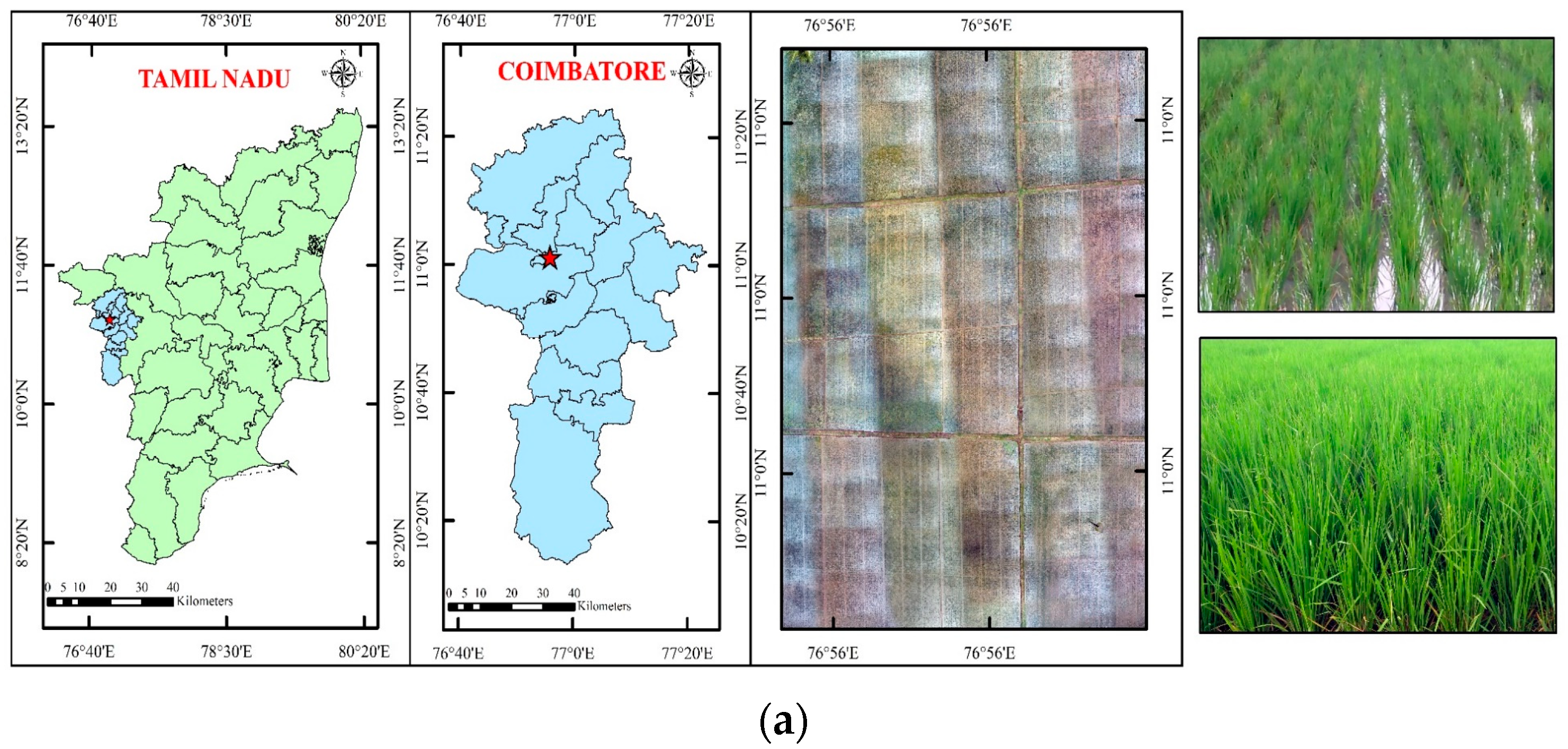
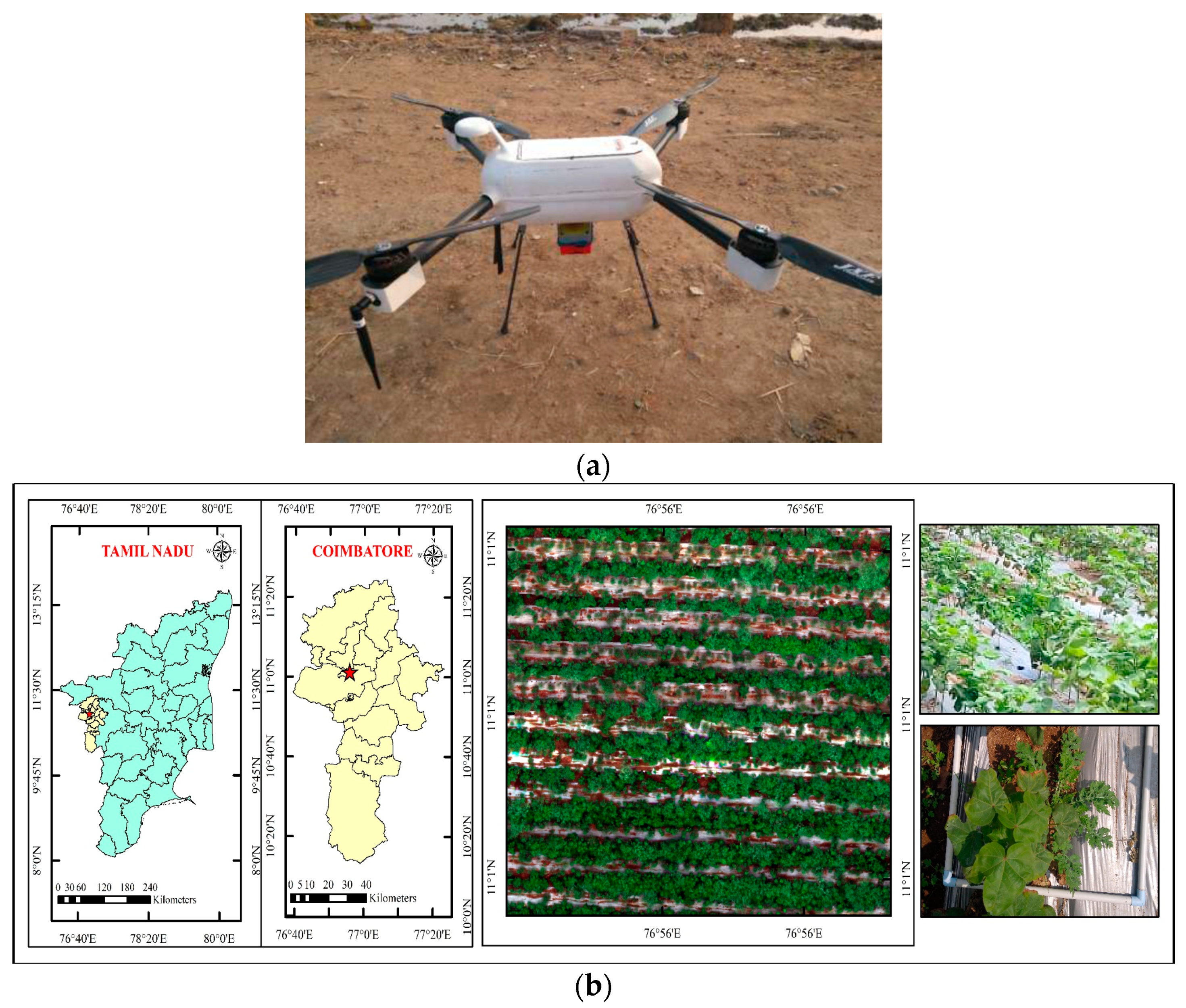
2.1. Study Area
2.2. Data Collection
2.2.1. Image Acquisition
2.2.2. Ground Data Collection
Leaf Area Index (LAI)
SPAD Chlorophyll
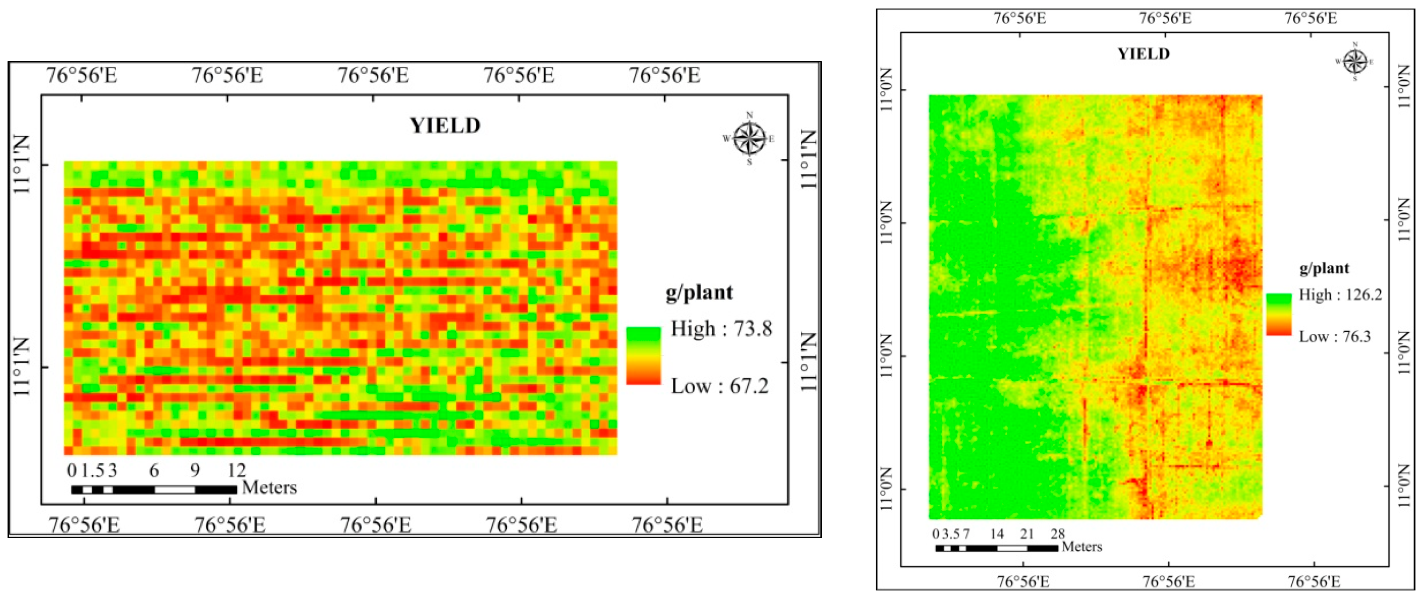
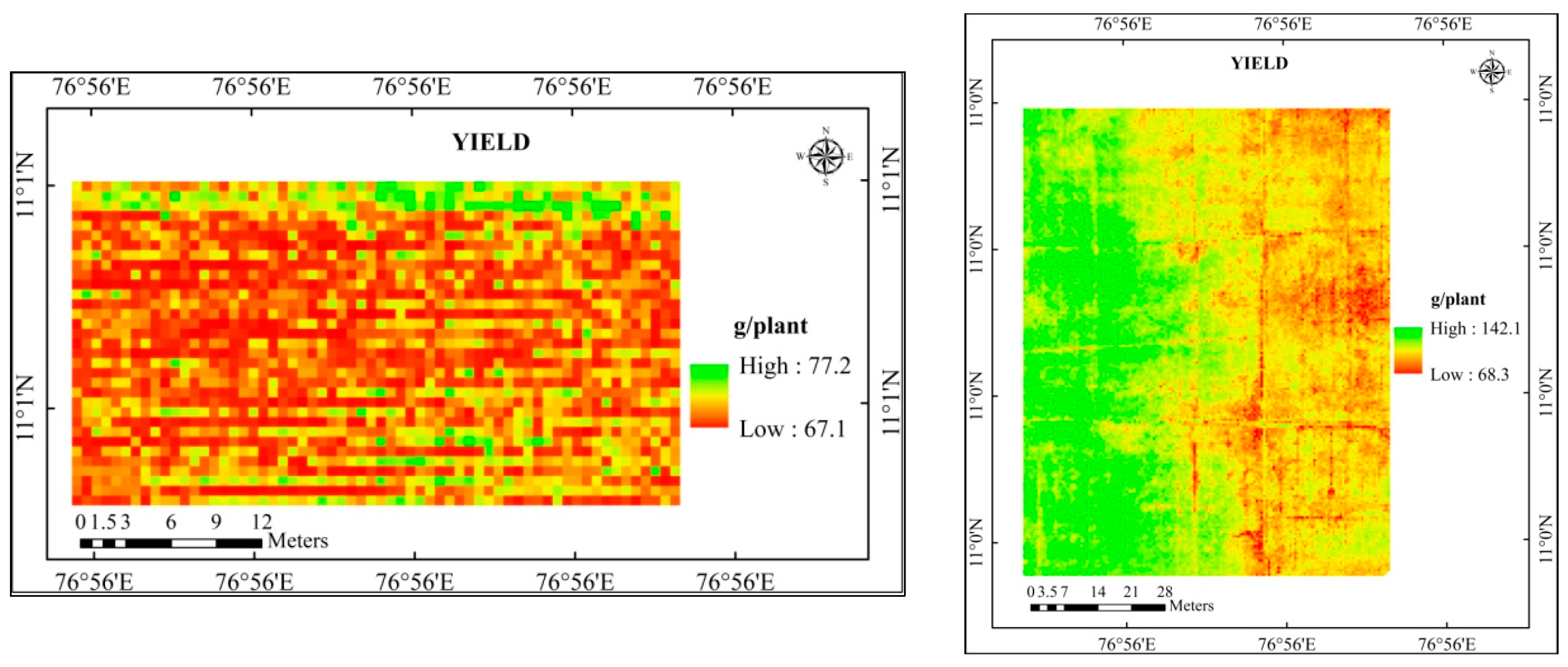
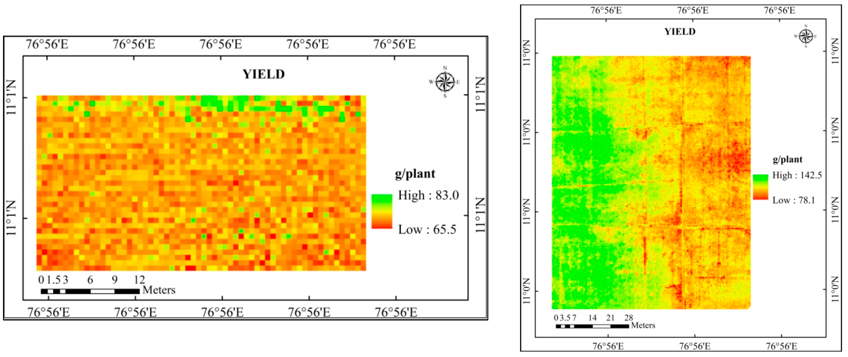
Yield (g/plant)
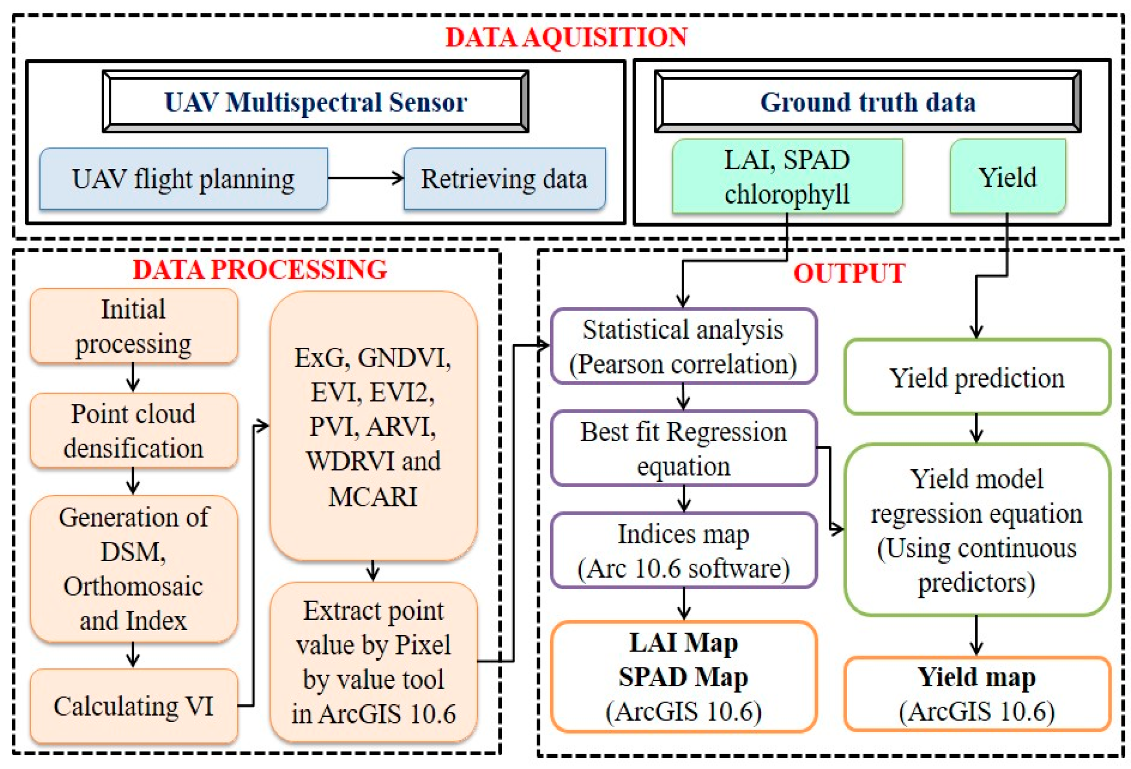
2.3. Data Processing
2.3.1. Image Processing
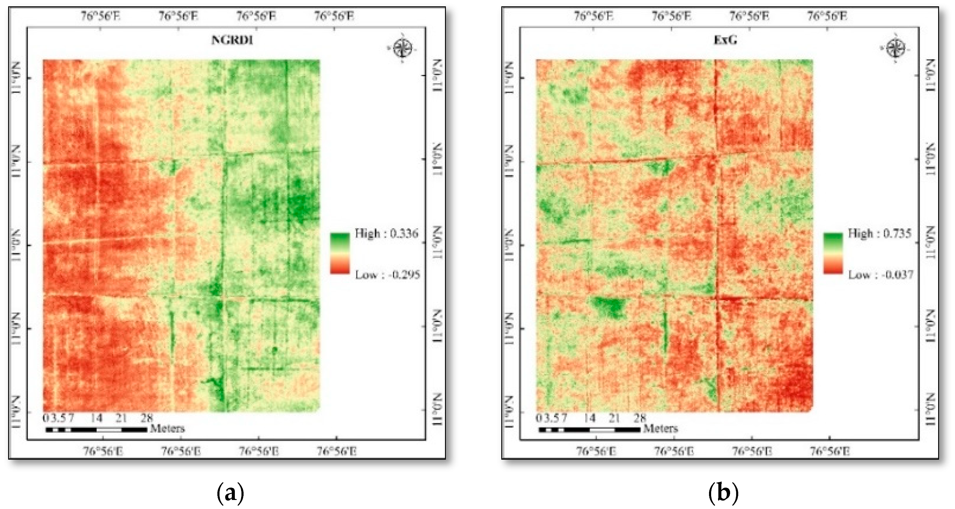
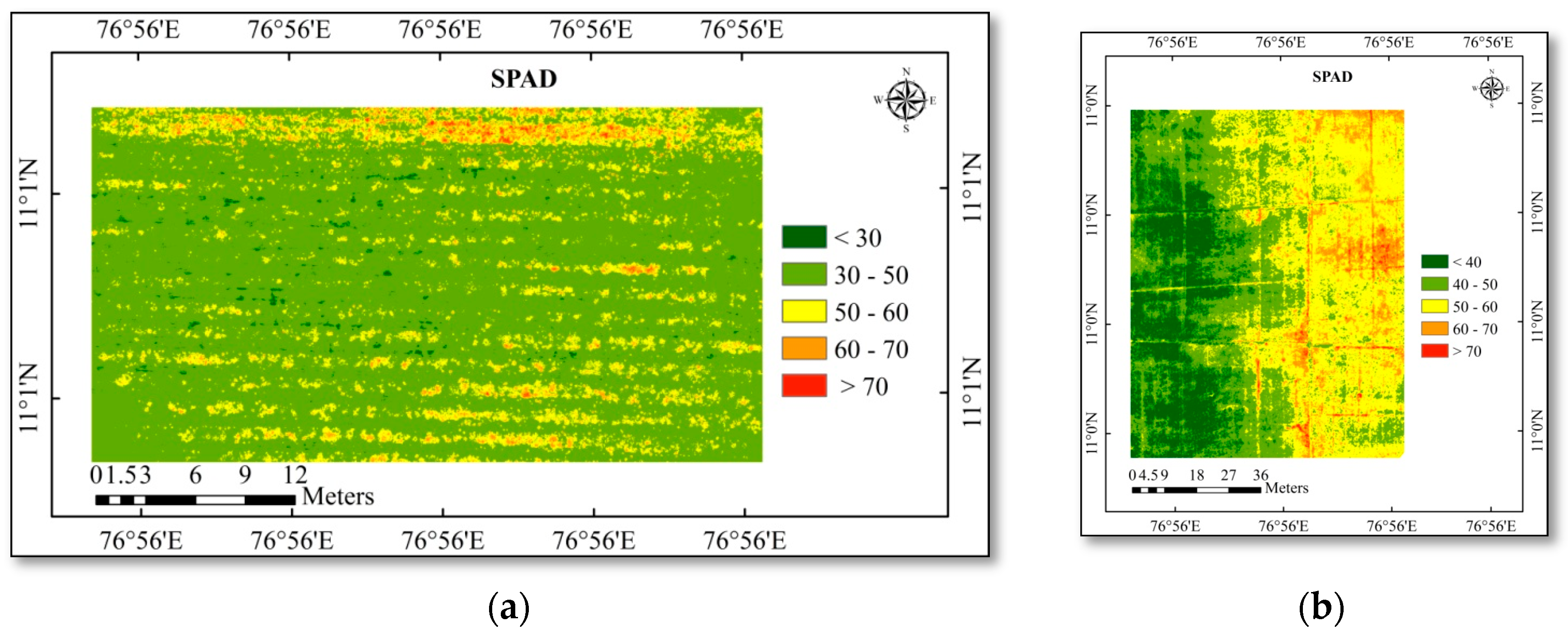
2.3.2. Vegetation Index Processing
2.4. Statistical Analysis
3. Results and Discussion
4. Conclusions
Author Contributions
Funding
Institutional Review Board Statement
Data Availability Statement
Acknowledgments
Conflicts of Interest
References
- Rani, A.; Chaudhary, A.; Sinha, N.; Mohanty, M.; Chaudhary, R. Drone: The green technology for future agriculture. Har. Dhara 2019, 2, 3–6. [Google Scholar]
- Tahir, M.N.; Naqvi, S.Z.A.; Lan, Y.; Zhang, Y.; Wang, Y.; Afzal, M.; Cheema, M.J.M.; Amir, S. Real time estimation of chlorophyll content based on vegetation indices derived from multispectral UAV in the kinnow orchard. Int. J. Precis. Agric. Aviat. 2018, 1, 24–31. [Google Scholar]
- Li, M.; Wu, J.; Song, C.; He, Y.; Niu, B.; Fu, G.; Tarolli, P.; Tietjen, B.; Zhang, X. Temporal variability of precipitation and biomass of alpine grasslands on the northern Tibetan plateau. Remote Sens. 2019, 11, 360. [Google Scholar] [CrossRef]
- Yang, G.; Liu, J.; Zhao, C.; Li, Z.; Huang, Y.; Yu, H.; Xu, B.; Yang, X.; Zhu, D.; Zhang, X. Unmanned aerial vehicle remote sensing for field-based crop phenotyping: Current status and perspectives. Front. Plant Sci. 2017, 8, 1111. [Google Scholar] [CrossRef]
- Tsouros, D.C.; Triantafyllou, A.; Bibi, S.; Sarigannidis, P.G. Data acquisition and analysis methods in UAV-based applications for Precision Agriculture. In Proceedings of the 2019 15th International Conference on Distributed Computing in Sensor Systems (DCOSS), Santorini Island, Greece, 29–31 May 2019; pp. 377–384. [Google Scholar]
- Maddikunta, P.K.R.; Hakak, S.; Alazab, M.; Bhattacharya, S.; Gadekallu, T.R.; Khan, W.Z.; Pham, Q.-V. Unmanned aerial vehicles in smart agriculture: Applications, requirements, and challenges. IEEE Sens. J. 2021, 21, 17608–17619. [Google Scholar] [CrossRef]
- Ballesteros, R.; Ortega, J.; Hernández, D.; Moreno, M. Applications of georeferenced high-resolution images obtained with unmanned aerial vehicles. Part I: Description of image acquisition and processing. Precis. Agric. 2014, 15, 579–592. [Google Scholar] [CrossRef]
- Nigon, T.J.; Mulla, D.J.; Rosen, C.J.; Cohen, Y.; Alchanatis, V.; Knight, J.; Rud, R. Hyperspectral aerial imagery for detecting nitrogen stress in two potato cultivars. Comput. Electron. Agric. 2015, 112, 36–46. [Google Scholar] [CrossRef]
- Delavarpour, N.; Koparan, C.; Nowatzki, J.; Bajwa, S.; Sun, X. A technical study on UAV characteristics for precision agriculture applications and associated practical challenges. Remote Sens. 2021, 13, 1204. [Google Scholar] [CrossRef]
- Tsouros, D.C.; Bibi, S.; Sarigiannidis, P.G. A review on UAV-based applications for precision agriculture. Information 2019, 10, 349. [Google Scholar] [CrossRef]
- Chu, T.; Chen, R.; Landivar, J.A.; Maeda, M.M.; Yang, C.; Starek, M.J. Cotton growth modeling and assessment using unmanned aircraft system visual-band imagery. J. Appl. Remote Sens. 2016, 10, 036018. [Google Scholar] [CrossRef]
- Duan, T.; Zheng, B.; Guo, W.; Ninomiya, S.; Guo, Y.; Chapman, S.C. Comparison of ground cover estimates from experiment plots in cotton, sorghum and sugarcane based on images and ortho-mosaics captured by UAV. Funct. Plant Biol. 2016, 44, 169–183. [Google Scholar] [CrossRef]
- Feng, A.; Zhang, M.; Sudduth, K.A.; Vories, E.D.; Zhou, J. Cotton yield estimation from UAV-based plant height. Trans. ASABE 2019, 62, 393–404. [Google Scholar] [CrossRef]
- Huang, Y.; Brand, H.J.; Sui, R.; Thomson, S.J.; Furukawa, T.; Ebelhar, M.W. Cotton yield estimation using very high-resolution digital images acquired with a low-cost small unmanned aerial vehicle. Trans. ASABE 2016, 59, 1563–1574. [Google Scholar]
- Liu, B.; Asseng, S.; Wang, A.; Wang, S.; Tang, L.; Cao, W.; Zhu, Y.; Liu, L. Modelling the effects of post-heading heat stress on biomass growth of winter wheat. Agric. For. Meteorol. 2017, 247, 476–490. [Google Scholar] [CrossRef]
- Quan, X.; He, B.; Yebra, M.; Yin, C.; Liao, Z.; Zhang, X.; Li, X. A radiative transfer model-based method for the estimation of grassland aboveground biomass. Int. J. Appl. Earth Obs. Geoinf. 2017, 54, 159–168. [Google Scholar] [CrossRef]
- Sun, Y.; Lu, L.; Liu, Y. Inversion of the leaf area index of rice fields using vegetation isoline patterns considering the fraction of vegetation cover. Int. J. Remote Sens. 2021, 42, 1688–1712. [Google Scholar] [CrossRef]
- Zhao, D.; Reddy, K.R.; Kakani, V.G.; Read, J.J.; Koti, S. Canopy reflectance in cotton for growth assessment and lint yield prediction. Eur. J. Agron. 2007, 26, 335–344. [Google Scholar] [CrossRef]
- Hunt, R. Plant Growth Curves: The Functional Approach to Plant Growth Analysis; Edward Arnold Ltd.: London, UK, 1982. [Google Scholar]
- Neupane, K.; Baysal-Gurel, F. Automatic identification and monitoring of plant diseases using unmanned aerial vehicles: A review. Remote Sens. 2021, 13, 3841. [Google Scholar] [CrossRef]
- Cao, J.; Gu, Z.; Xu, J.; Duan, Y.; Liu, Y.; Liu, Y.; Li, D. Sensitivity analysis for leaf area index (LAI) estimation from CHRIS/PROBA data. Front. Earth Sci. 2014, 8, 405–413. [Google Scholar] [CrossRef]
- Shang, J.; Liu, J.; Ma, B.; Zhao, T.; Jiao, X.; Geng, X.; Huffman, T.; Kovacs, J.M.; Walters, D. Mapping spatial variability of crop growth conditions using RapidEye data in Northern Ontario, Canada. Remote Sens. Environ. 2015, 168, 113–125. [Google Scholar] [CrossRef]
- Towers, P.C.; Strever, A.; Poblete-Echeverría, C. Comparison of vegetation indices for leaf area index estimation in vertical shoot positioned vine canopies with and without grenbiule hail-protection netting. Remote Sens. 2019, 11, 1073. [Google Scholar] [CrossRef]
- Bajwa, S.G.; Rupe, J.C.; Mason, J. Soybean disease monitoring with leaf reflectance. Remote Sens. 2017, 9, 127. [Google Scholar] [CrossRef]
- Maresma, Á.; Ariza, M.; Martínez, E.; Lloveras, J.; Martínez-Casasnovas, J.A. Analysis of vegetation indices to determine nitrogen application and yield prediction in maize (Zea mays L.) from a standard UAV service. Remote Sens. 2016, 8, 973. [Google Scholar] [CrossRef]
- Hunt, E.R.; Cavigelli, M.; Daughtry, C.S.; Mcmurtrey, J.E.; Walthall, C.L. Evaluation of digital photography from model aircraft for remote sensing of crop biomass and nitrogen status. Precis. Agric. 2005, 6, 359–378. [Google Scholar] [CrossRef]
- Li, W.; Niu, Z.; Chen, H.; Li, D.; Wu, M.; Zhao, W. Remote estimation of canopy height and aboveground biomass of maize using high-resolution stereo images from a low-cost unmanned aerial vehicle system. Ecol. Indic. 2016, 67, 637–648. [Google Scholar] [CrossRef]
- Bendig, J.; Yu, K.; Aasen, H.; Bolten, A.; Bennertz, S.; Broscheit, J.; Gnyp, M.L.; Bareth, G. Combining UAV-based plant height from crop surface models, visible, and near infrared vegetation indices for biomass monitoring in barley. Int. J. Appl. Earth Obs. Geoinf. 2015, 39, 79–87. [Google Scholar] [CrossRef]
- Pandit, S.; Tsuyuki, S.; Dube, T. Landscape-scale aboveground biomass estimation in buffer zone community forests of central Nepal: Coupling in situ measurements with Landsat 8 satellite data. Remote Sens. 2018, 10, 1848. [Google Scholar] [CrossRef]
- Lee, D.-H.; Shin, H.-S.; Park, J.-H. Developing a p-NDVI map for highland kimchi cabbage using spectral information from UAVs and a field spectral radiometer. Agronomy 2020, 10, 1798. [Google Scholar] [CrossRef]
- Delegido, J.; Verrelst, J.; Meza, C.; Rivera, J.; Alonso, L.; Moreno, J. A red-edge spectral index for remote sensing estimation of green LAI over agroecosystems. Eur. J. Agron. 2013, 46, 42–52. [Google Scholar] [CrossRef]
- Gitelson, A.A. Wide dynamic range vegetation index for remote quantification of biophysical characteristics of vegetation. J. Plant Physiol. 2004, 161, 165–173. [Google Scholar] [CrossRef]
- Ashapure, A.; Jung, J.; Chang, A.; Oh, S.; Maeda, M.; Landivar, J. A comparative study of RGB and multispectral sensor-based cotton canopy cover modelling using multi-temporal UAS data. Remote Sens. 2019, 11, 2757. [Google Scholar] [CrossRef]
- Shamshiri, R.R.; Mahadi, M.R.; Ahmad, D.; Bejo, S.K.; Aziz, S.A.; Ismail, W.I.W.; Che Man, H. Controller design for an osprey drone to support precision agriculture research in oil palm plantations. In Proceedings of the 2017 ASABE Annual International Meeting, Spokane, DC, USA, 16–19 July 2017; pp. 2–13. [Google Scholar]
- Gitelson, A.A.; Viña, A.; Verma, S.B.; Rundquist, D.C.; Arkebauer, T.J.; Keydan, G.P.; Leavitt, B.; Ciganda, V.S.; Burba, G.; Suyker, A.E.; et al. Relationship between gross primary production and chlorophyll content in crops: Implications for the synoptic monitoring of vegetation productivity. J. Geophys. Res. Atmos. 2006, 111, D8. [Google Scholar] [CrossRef]
- Raper, T.B.; Varco, J.J. Canopy-scale wavelength and vegetative index sensitivities to cotton growth parameters and nitrogen status. Precis. Agric. 2015, 16, 62–76. [Google Scholar] [CrossRef]


| SL. No. | Crop | Area (Acres) | Latitude | Longitude | Above MSL (m) |
|---|---|---|---|---|---|
| 1 | Cotton | 0.5 | 11°01′15″ N to 11°01′14″ N | 76°55′48″ E to 76°55′49″ E | 430 |
| 2 | Rice | 1.5 | 11°00′14″ N to 11°00′11″ N | 76°55′37″ E to 76°55′39″ E | 418 |
| Platform | Quadcopter |
| Flight speed (m s−1) | 8 |
| Flight altitude (m) | 30 |
| Per cent overlap | 70 |
| Ground Sample Distance (GSD) | 5 cm per pixel (per band) |
| Sensor model | Mica Sense Red Edge |
| Spectral Bands | Blue, green, red, red edge, near-IR |
| Wavelength (nm) | Blue (475 nm center, 20 nm bandwidth), green (560 nm center, 20 nm bandwidth), red (668 nm center, 10 nm bandwidth), red edge (717 nm center, 10 nm bandwidth) and near-IR (840 nm center, 40 nm bandwidth) |
| Sensor size/mm | 23.5 × 15.6 |
| Image resolution (pixels) | 4000 × 6000 |
| Cotton | ||
|---|---|---|
| Indices | Formula | Applications and Reference |
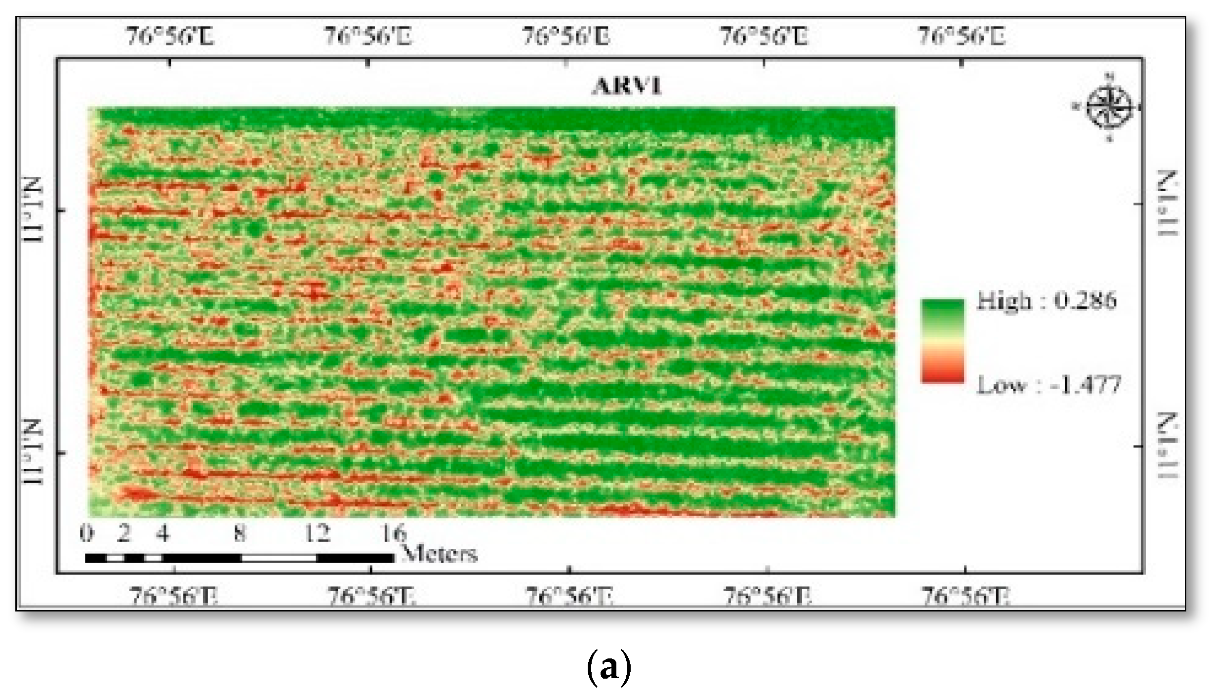
| ARVI | LAI estimation [21] | |
| MCARI | Chlorophyll content [22] | |
| WDRVI | N-Application, LAI [23], disease infestation [24], and yield estimation [25] | |
| Rice | ||
| NGRDI | Chlorophyll content, biomass, and water content estimation [26] | |
| ExG | 2g – r – b | Green features and vegetation cover [27] |
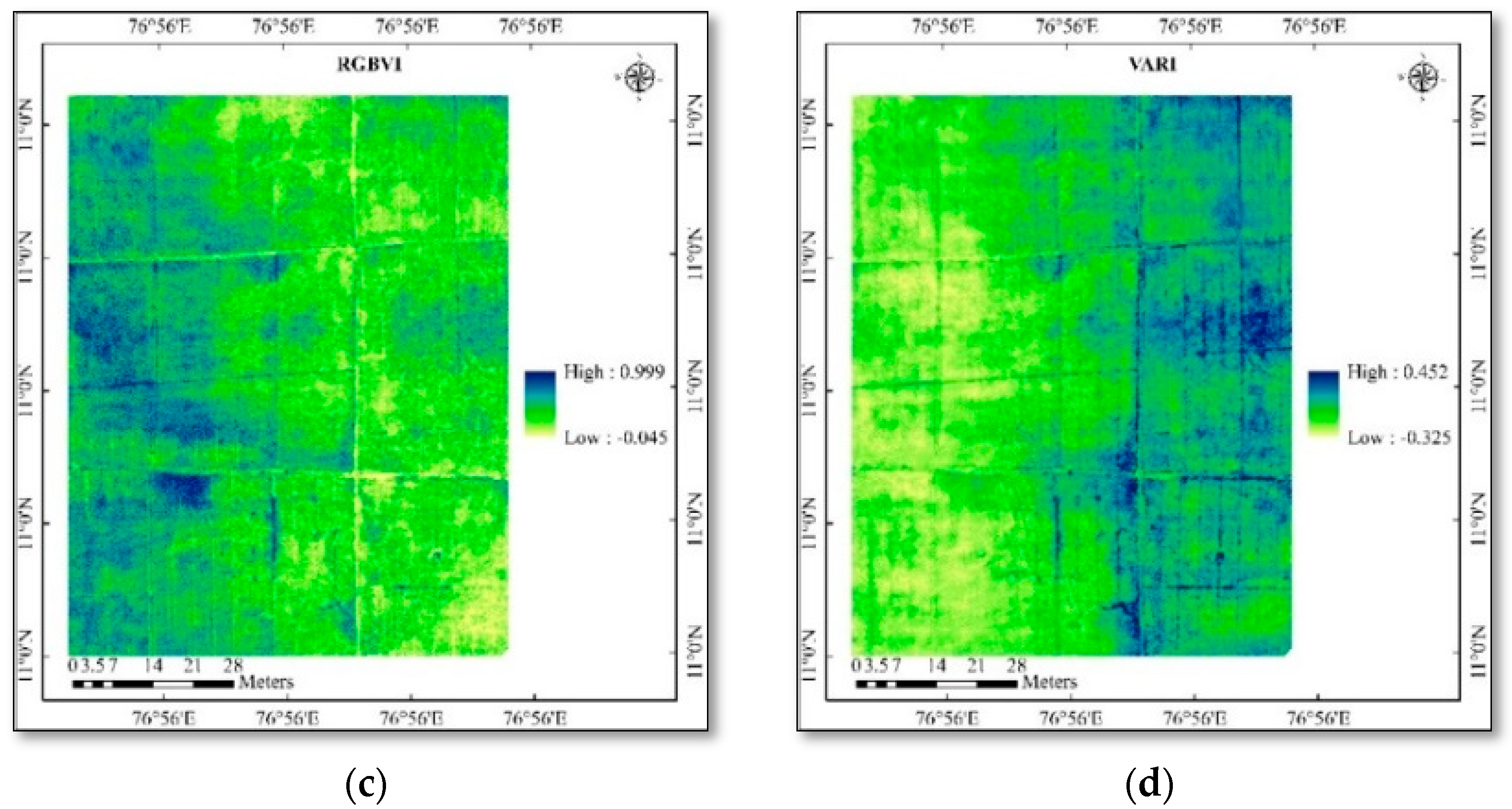
| RGBVI | Biomass estimation [28] | |
| VARI | Fraction of vegetation cover [29] | |
| S.No. | Latitude | Longitude | LAI | SPAD Value | ARVI | MCARI | WDRVI | Seed Cotton Yield (g/Plant) |
|---|---|---|---|---|---|---|---|---|
| 1. | 11.0208 | 76.9302 | 1.2 | 57.6 | 0.786 | 0.505 | −0.052 | 76 |
| 2. | 11.0208 | 76.9305 | 0.9 | 42.4 | 0.721 | 0.225 | −0.17 | 67 |
| 3. | 11.0208 | 76.9302 | 0.7 | 44.5 | 0.581 | 0.175 | −0.375 | 68 |
| 4. | 11.0208 | 76.9302 | 0.8 | 38.1 | 0.686 | 0.21 | −0.247 | 70 |
| 5. | 11.0208 | 76.9305 | 1.0 | 51.9 | 0.767 | 0.319 | −0.146 | 75 |
| 6. | 11.0208 | 76.9303 | 1.4 | 56.1 | 0.813 | 0.438 | 0.023 | 73 |
| 7. | 11.0208 | 76.9303 | 1.3 | 55.1 | 0.793 | 0.368 | −0.032 | 71 |
| 8. | 11.0208 | 76.9303 | 1.0 | 48.6 | 0.737 | 0.298 | −0.16 | 75 |
| 9. | 11.0207 | 76.9303 | 1.7 | 60.5 | 0.845 | 0.474 | 0.058 | 70 |
| 10. | 11.0208 | 76.9302 | 0.8 | 45.6 | 0.624 | 0.262 | −0.297 | 70 |
| S.No. | Latitude | Longitude | LAI | SPAD Value | NGRDI | ExG | RGBVI | VARI | Yield (g/Plant) |
|---|---|---|---|---|---|---|---|---|---|
| 1. | 11.0038 | 76.9272 | 2.5 | 34.2 | −0.092 | 0.115 | 0.26 | −0.118 | 117 |
| 2. | 11.0038 | 76.9274 | 2.9 | 47.6 | 0.013 | 0.191 | 0.306 | 0.018 | 104 |
| 3. | 11.0040 | 76.9274 | 2.8 | 59.7 | −0.029 | 0.079 | 0.133 | −0.045 | 87 |
| 4. | 11.0037 | 76.9273 | 2.7 | 39.4 | −0.038 | 0.104 | 0.183 | −0.054 | 107 |
| 5. | 11.0038 | 76.9276 | 3.2 | 59.7 | 0.052 | 0.182 | 0.271 | 0.078 | 112 |
| 6. | 11.0040 | 76.9276 | 3.1 | 54.9 | 0.037 | 0.076 | 0.113 | 0.068 | 86 |
| 7. | 11.0040 | 76.9272 | 2.6 | 36.4 | −0.061 | 0.152 | 0.303 | −0.079 | 122 |
| 8. | 11.0037 | 76.9272 | 2.6 | 35.6 | −0.077 | 0.156 | 0.335 | −0.096 | 131 |
| 9. | 11.0040 | 76.9271 | 2.9 | 40.2 | −0.029 | 0.222 | 0.41 | −0.036 | 134 |
| 10. | 11.0037 | 76.9276 | 3.3 | 57.9 | 0.047 | 0.105 | 0.154 | 0.082 | 97 |
| Correlation Matrix | LAI | SPAD | ||
|---|---|---|---|---|
| Cotton | ARVI | 0.905 | ARVI | 0.791 |
| WDRVI | 0.955 | MCARI | 0.931 | |
| Rice | RGBVI | −0.433 | NGRDI | 0.844 |
| VARI | 0.982 | ExG | −0.292 | |
| Plant Attributes | Indices | Crop | Regression Equation | R2 | RMSE |
|---|---|---|---|---|---|
| LAI | WDRVI | Cotton | y = 2.0913x + 1.3744 | 0.911 | 0.097 |
| VARI | Rice | y = 3.4089x + 2.9286 | 0.965 | 0.051 | |
| SPAD | MCARI | Cotton | y = 59.277x + 30.639 | 0.866 | 2.851 |
| NGRDI | Rice | y = 171.31x + 49.583 | 0.712 | 6.034 |
| Correlation Matrix | Predicted Values | ||
|---|---|---|---|
| LAI | SPAD | ||
| Observed values | Cotton | R = 0.844 | R = 0.880 |
| Rice | R = 0.803 | R = 0.830 | |
| Attributes | Regression Equation | R2 | RMSE |
|---|---|---|---|
| Cotton | |||
| LAI | Y = 68.41 + 2.94 LAI | 0.093 | 3.060 |
| SPAD | Y = 60.80 + 0.215 SPAD | 0.272 | 2.741 |
| LAI + SPAD | Y = 55.04 + 0.481 SPAD − 6.99 LAI | 0.387 | 2.690 |
| Rice | |||
| LAI | Y = 192.9 − 29.1 LAI | 0.222 | 15.692 |
| SPAD | Y = 164.9 − 1.185 SPAD | 0.561 | 11.783 |
| LAI + SPAD | Y = 108.4 − 1.827 SPAD + 30.2 LAI | 0.635 | 11.485 |
| RMSE, NRMSE, and Agreement | ||||||||
|---|---|---|---|---|---|---|---|---|
| Attributes | Cotton Crop Area (m2) = 864.44 and Actual Yield (kg) = 130 Rice Crop Area (m2) = 7496.25 and Actual Yield (kg) = 3100 | |||||||
| Predicted Yield (kg) | RMSE (kg/ha) | NRMSE (%) | Agreement (%) | |||||
| Cotton | Rice | Cotton | Rice | Cotton | Rice | Cotton | Rice | |
| LAI | 144.57 | 3082.36 | 14.57 | 917.64 | 11.21 | 22.94 | 88.8 | 77.1 |
| SPAD | 142.05 | 3104.35 | 12.05 | 895.65 | 9.27 | 22.39 | 90.7 | 77.6 |
| SPAD + LAI | 139.42 | 3104.13 | 9.42 | 895.87 | 7.25 | 22.40 | 92.8 | 77.6 |
Disclaimer/Publisher’s Note: The statements, opinions and data contained in all publications are solely those of the individual author(s) and contributor(s) and not of MDPI and/or the editor(s). MDPI and/or the editor(s) disclaim responsibility for any injury to people or property resulting from any ideas, methods, instructions or products referred to in the content. |
© 2023 by the authors. Licensee MDPI, Basel, Switzerland. This article is an open access article distributed under the terms and conditions of the Creative Commons Attribution (CC BY) license (https://creativecommons.org/licenses/by/4.0/).
Share and Cite
Pazhanivelan, S.; Kumaraperumal, R.; Shanmugapriya, P.; Sudarmanian, N.S.; Sivamurugan, A.P.; Satheesh, S. Quantification of Biophysical Parameters and Economic Yield in Cotton and Rice Using Drone Technology. Agriculture 2023, 13, 1668. https://doi.org/10.3390/agriculture13091668
Pazhanivelan S, Kumaraperumal R, Shanmugapriya P, Sudarmanian NS, Sivamurugan AP, Satheesh S. Quantification of Biophysical Parameters and Economic Yield in Cotton and Rice Using Drone Technology. Agriculture. 2023; 13(9):1668. https://doi.org/10.3390/agriculture13091668
Chicago/Turabian StylePazhanivelan, Sellaperumal, Ramalingam Kumaraperumal, P. Shanmugapriya, N. S. Sudarmanian, A. P. Sivamurugan, and S. Satheesh. 2023. "Quantification of Biophysical Parameters and Economic Yield in Cotton and Rice Using Drone Technology" Agriculture 13, no. 9: 1668. https://doi.org/10.3390/agriculture13091668
APA StylePazhanivelan, S., Kumaraperumal, R., Shanmugapriya, P., Sudarmanian, N. S., Sivamurugan, A. P., & Satheesh, S. (2023). Quantification of Biophysical Parameters and Economic Yield in Cotton and Rice Using Drone Technology. Agriculture, 13(9), 1668. https://doi.org/10.3390/agriculture13091668