Development of a Control System for Double-Pendulum Active Spray Boom Suspension Based on PSO and Fuzzy PID

Abstract

During the operation of boom sprayers in the field, it is crucial to ensure that the entire boom is maintained at an optimal height relative to the ground or crop canopy. Active suspension is usually used to adjust the height. A control system for double-pendulum active suspension was developed in this paper. The control system consisted of a main control node, two distance measurement nodes, a vehicle inclination detection node, and an execution node. Communication between nodes was carried out using a CAN bus. The hardware was selected, and the interface circuits of the sensors and the actuator were designed. The transfer functions of the active suspension and electric linear actuator were established. In order to enhance the efficiency of the control system, the particle swarm optimization (PSO) algorithm was employed to optimize the initial parameters of the fuzzy PID controller. The simulation results demonstrated that the PSO-based fuzzy PID controller exhibited improvements in terms of reduced overshoot and decreased settling time when compared to conventional PID and fuzzy PID controllers. The experimental results showed that the active suspension system equipped with the control system could effectively isolate high-frequency disturbances and follow low-frequency ground undulations, meeting the operational requirements.

1. Introduction

Boom sprayers are commonly used in crop protection to apply chemical materials that prevent diseases, weeds, and other problems due to their wide coverage and high efficiency [1,2,3]. Tractor vibrations and uneven field terrain may cause undesired boom motions, such as rolling, yawing, and jolting [4,5]. These boom motions have negative effects on the distribution of spray deposits [6,7]. Studies have shown that boom rolling in the vertical plane is accountable for variations in the distribution of spray deposits ranging from 0 to 1000%, with the optimum amount being 100% [8,9]. Therefore, booms are typically mounted with a vertical suspension system to reduce rolling for the majority of sprayers [10]. There have been many types of vertical suspension systems, including pendulum suspension, trapezium suspension, cable suspension, and Douven suspension [11,12,13,14,15]. Double-pendulum suspension systems have been studied over the past few years, both theoretically and experimentally [16,17,18,19,20]. In these studies, various control methods, including proportional, proportional-integral, and H^∞ control theory, have been tested to regulate the motion of the boom. Modern large and medium-sized sprayers have achieved electromechanical–hydraulic integration control. They utilize computers to perform the real-time monitoring and adjustment of operational speed, spray volume, spray pressure, and other parameters. The spray boom’s position and balance are achieved through a hydraulic system. The UC5 boom height controller produced by NORAC, a Canadian company, consists of ultrasonic sensors, roll sensors, control modules, proportional valves, display terminals, and bus terminators. Using sensor data, it can make responsive height adjustments, allowing the boom to automatically follow the contours of the land. The CONTOUR system developed by the UK company Cheffer can quickly level 18 m and 24 m long booms, enhancing the operational efficiency and spraying accuracy of the sprayer.

Manufacturers and researchers have developed different types of control systems that can automatically adjust the height between the boom and the ground or the crop canopy. Xue et al. developed a control method based on an adaptive fuzzy sliding model control algorithm. The method exhibited superior responsiveness, stability, and accuracy when compared to conventional PID control [21]. Cui et al. designed a high-performance boom control system for conventional pendulum active suspension based on a digital signal processor. The speed feed-forward compensation PID control method was used to achieve the high-precision control of the spray boom [22]. Aiming at the problem of low accuracy and poor stability caused by parameter uncertainties in the suspension and the electro-hydraulic position servo system, Cui et al. studied an adaptive robust controller based on a nonlinear model of the suspension system. The proposed controller demonstrated good asymptotic tracking performance and steady-state tracking accuracy when compared to the feedback linearization controller, robust feedback controller, and PID controller [23]. These control systems adopt hydraulic cylinders as actuators and require specific machine configurations to operate effectively. In recent years, attempts have been made to control the motion of spray booms using microcontroller units and programmable logic controllers. However, the control effects were unsatisfactory due to their limitations [24,25].

In this study, an electric linear actuator was employed, thereby simplifying the configuration of the control system. The control system for the inclination angle of the boom was designed based on a CAN bus. The control algorithm was developed based on PSO and fuzzy PID. Finally, the effectiveness of the control system was verified by experiments using double-pendulum active suspension.

2. Modeling of the Double-Pendulum Suspension System

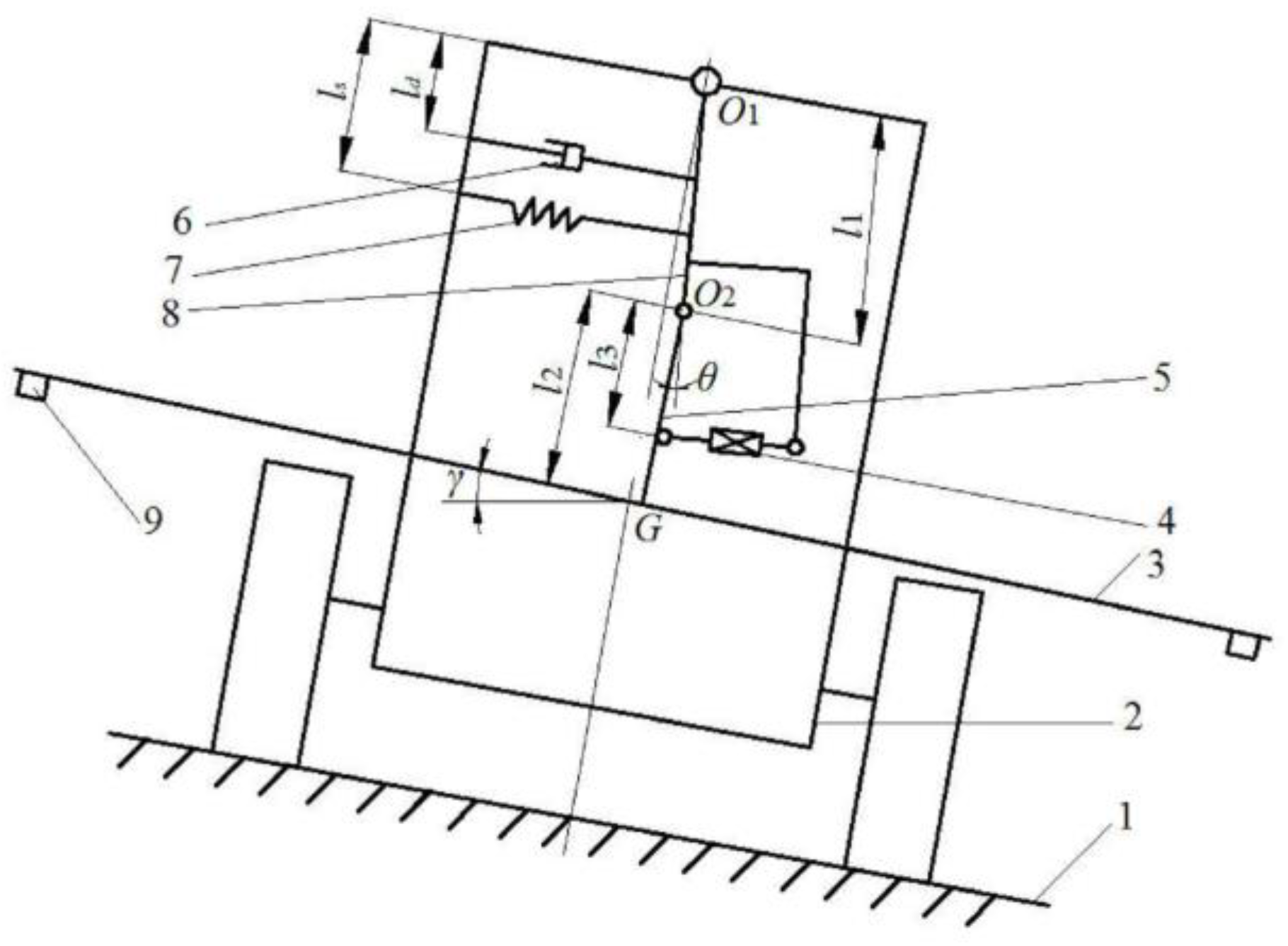
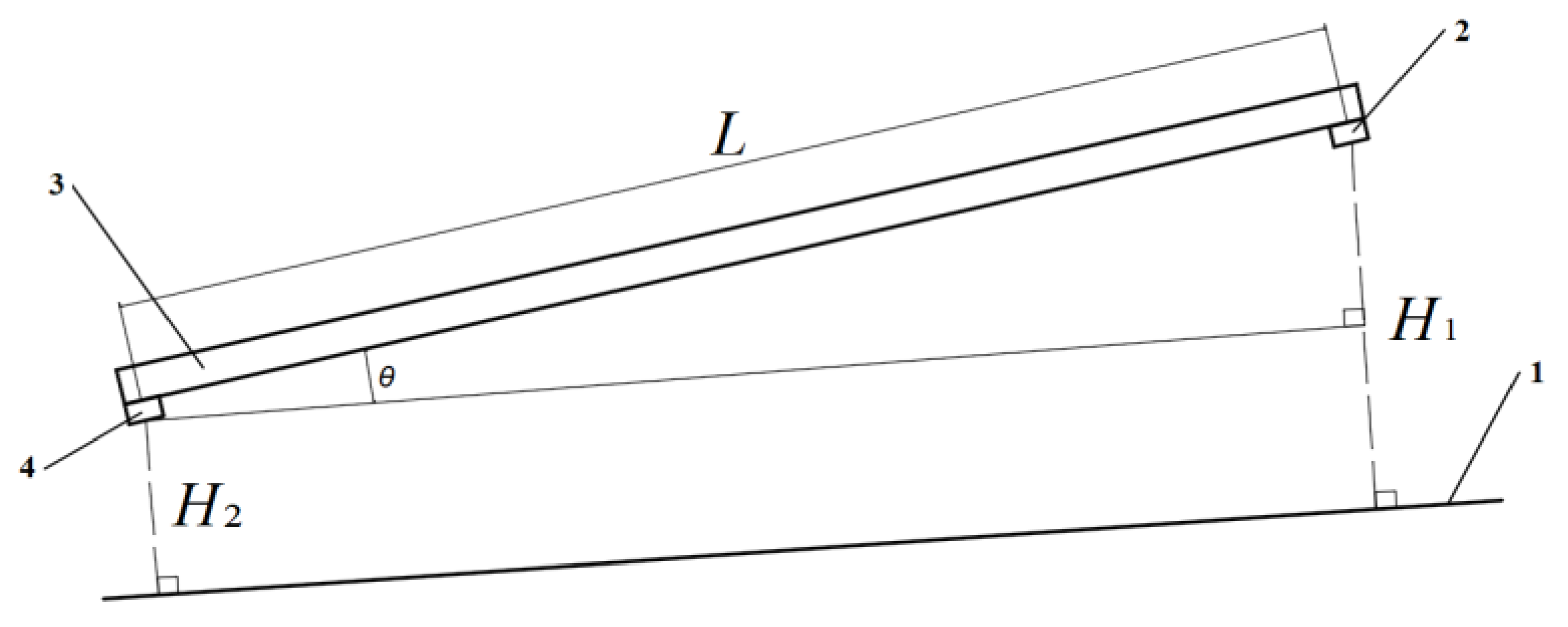
2.1. Description of the Suspension System

A double-pendulum suspension system is comprised of two pendulum rods, height sensors, springs, dampers, and an actuator, as illustrated in Figure 1. The first pendulum rod is articulated to the frame and the second pendulum rod at O₁ and O₂, respectively. The boom is rigidly fixed to the second pendulum rod at G, the gravity center of the boom. A spring and a damper are connected between the first pendulum rod and the frame attached to the vehicle. An actuator is installed between the first and second pendulum rods.

In the event that the power supply is deactivated and the actuator length remains constant, the suspension becomes passive, causing the boom to pivot only around O₁. A special case arises when the angle between the first and second pendulum rods is zero, indicating that the boom’s balance position is horizontal, with its gravity center G below the hinge point O₁. However, if the actuator length is either increased or decreased, the boom’s gravity center will shift to the left or right, respectively, resulting in a non-horizontal equilibrium position. Consequently, by continuously regulating the actuator length, the suspension becomes active, enabling the boom to adapt to variations in ground slope.

2.2. Transfer Function of the Active Suspension System

The suspension system’s parameters are presented in Figure 1. For the control of active suspension, the input is the actuator displacement d, and the output is the inclination angle of the boom γ. For the generalized coordinate γ, by applying the second Lagrange equation, the equation of the boom motion can be derived as

$$\frac{d}{dt}\left(\frac{\partial E_k}{\partial \dot{\gamma }}\right)-\frac{\partial E_k}{\partial \gamma }=Q_{\gamma }-\frac{\partial \psi }{\partial \dot{\gamma }},$$

(1)

where E_k represents the kinetic energy of the boom (in N·m); γ represents the inclination angle of the boom (rad); Q_γ represents the generalized force (N); and ψ represents the dissipation function (N·m·rad/s).

The kinetic energy of the boom can be expressed as

$$E_k=\frac{1}{2}I{\dot{\gamma }}^2+\frac{1}{2}m{\left[(l_1+l_2)\dot{\gamma }-l_1\dot{\theta }\right]}^2,$$

(2)

where I represents the moment of inertia of the boom about the axis through G (kg·m²); m represents the mass of the boom (kg); l₁ represents the length of the first pendulum (m); l₂ represents the length of the second pendulum (m); and θ represents the angle between the first and second pendulum rods (rad).

Based on Equation (2), the following two equations can be inferred:

$$\frac{d}{dt}\left(\frac{\partial E_k}{\partial \dot{\gamma }}\right)=[I+m{(l_1+l_2)}^2]\ddot{\gamma }-m{l}_1(l_1+l_2)\ddot{\theta }$$

(3)

$$\frac{\partial E_k}{\partial \gamma }=0$$

(4)

The generalized force can be expressed as

$$Q_{\gamma }=(mg{l}_1-k{l}_s{}^2)(d/l_3-\gamma ),$$

(5)

where k represents the stiffness coefficient of the spring (N/m); l_s represents the distance from the spring’s installation position to O₁ (m); d represents the actuator displacement (m); and l₃ represents the distance between the installation position of the actuator and the point O₂ (m).

The dissipation function can be expressed as

$$\psi =c{l}_d{}^2{(\dot{\theta }-\dot{\gamma })}^2/2,$$

(6)

where c represents the damping coefficient of the damper (N·s/m), and l_d represents the distance from the damper’s installation position to O₁ (m).

Therefore,

$$\frac{\partial \psi }{\partial \dot{\gamma }}=-c{l}_d{}^2(\dot{\theta }-\dot{\gamma })$$

(7)

Assuming that γ and d are small, ignoring the second-order terms, and substituting Equations (3)–(5) and (7) into Equation (1), the equation of the boom motion can be stated in the following form:

$$l_3[(I+m{(l_1+l_2)}^2)]\ddot{\gamma }+l_{3}c{l}_d{}^2\dot{\gamma }+l_3(mg{l}_1-k{l}_s{}^2)=m{l}_1(l_1+l_2)\ddot{d}+c{l}_d{}^2\dot{d}+(mg{l}_1-k{l}_s{}^2)d$$

(8)

By performing the Laplace transform on Equation (8) and rearranging the terms, the transfer function linking the inclination angle of the boom, γ, to the actuator displacement, d, can be derived as

$$G(s)=\frac{\gamma (s)}{d(s)}=\frac{m{l}_1(l_1+l_2)s^2+c{l}_d{}^{2}s+(mg{l}_1-k{l}_s{}^2)}{l_3[(I+m{(l_1+l_2)}^2)]s^2+l_{3}c{l}_d{}^{2}s+l_3(mg{l}_1-k{l}_s{}^2)}.$$

(9)

2.3. Transfer Function of the Electric Linear Actuator

In this study, a DC electric linear actuator was chosen as the actuator. Compared with pneumatic cylinders and hydraulic cylinders, it has the advantages of lower price, smaller size, lighter weight, easier installation, and no need for air source or oil circuit. It also has good mechanical characteristics, sensitive movement, and is convenient for electrical control. The controller generates PWM (pulse width modulation) pulses with a certain duty cycle, which are sent to the motor driver. The driver regulates the input voltage and generates an output voltage proportional to the duty cycle, which is subsequently transmitted to the electric linear actuator.

The transfer function of the electric linear actuator can be expressed as

$$G_m(s)=\frac{d(s)}{R(s)}=\frac{K}{s(Ts+1)},$$

(10)

where d(s) represents the image function of the displacement of the actuator piston rod, R(s) represents the image function of the duty cycle, K represents the proportionality coefficient, and T represents the time constant [26,27,28].

To obtain the parameters of the transfer function, we adopted the time domain identification method to model the electric linear actuator. A step signal was applied, and the response curve of the piston rod displacement over time was measured.

The equipment for determining the parameters is shown in Figure 2. In order to reduce the impact of random disturbances on the measurement error, a single-chip microcomputer was used to emit a pulse with a frequency of 20 kHz and a duty cycle of 100% as the input signal. The driver modulated the input 24 V voltage to form an output voltage, which was supplied to the electric linear actuator. The displacement of the actuator piston rod was measured using a linear displacement sensor, and the voltage signal output by the sensor was input into a data acquisition device and saved on a computer.

In order to obtain the displacement of the actuator piston rod, the linear displacement sensor was calibrated before the measurement. By fitting the experimental data, the fitted equation between the actuator piston rod displacement d and the sensor output voltage u was obtained as d = 21.108u + 0.3854, with a coefficient of determination R² = 0.9815.

According to Equation (10), the step response of the actuator piston rod velocity can be represented by the following equation:

$$v(t)=K(1-{\mathrm{e}}^{-t/T}),$$

(11)

where v(t) represents the actuator piston rod velocity (mm/s), and t represents time (s).

Based on the measured displacement of the actuator piston rod, the velocity response of the actuator piston rod was obtained by numerical differentiation. Then, K and T were determined by numerical fitting, and the results are shown in Figure 3.

Using the MATLAB fitting toolbox, the fitted equation was obtained as v(t) = 11.49(1 − e^−t/0.085), with a coefficient of determination R² = 0.89. Therefore, it could be concluded that K = 11.49 and T = 0.085 in the transfer function.

3. Design of the Control System

3.1. Design of the Control System Hardware

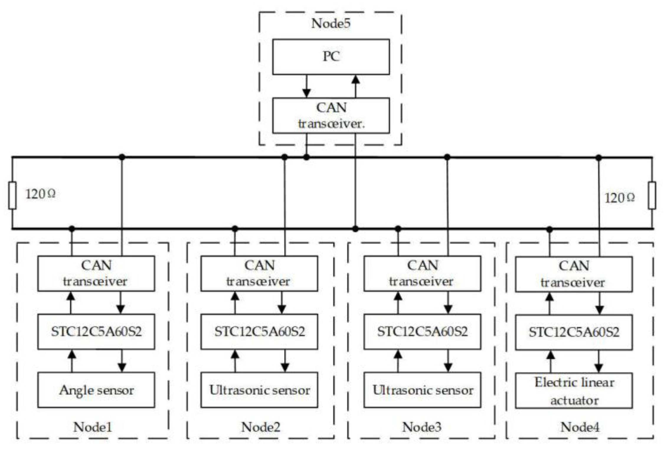
3.1.1. Overall Structure of the Control System

The control system consisted of a computer, four single-chip microcomputers, and communication lines, as shown in Figure 4. Node 1 was used to measure the inclination angle of the vehicle body, nodes 2 and 3 were used to measure the distance between the spray boom and crop canopy or ground, and node 4 was used to drive the actuator. The CPU of each node used a high-integration and strong anti-interference single-chip microcontroller. Node 5, the computer node, was mainly responsible for analyzing the data transmitted by each node and issuing commands to the actuator according to the analysis results.

3.1.2. Hardware Selection

(1)

Main control chips of the functional nodes

The main control chips need to be installed on the spray boom, which requires a small size and strong anti-interference ability in complex field conditions. Considering the above factors, the STC12C5A60S2 microcomputer produced by Shenzhen Hongjing Company was chosen. It has a faster execution speed than microcomputers with the same frequency. It also integrates an eight-channel 10-bit voltage input successive comparison high-speed analog-to-digital converter. Unlike ordinary 51-series microcomputers, it integrates two UART full-duplex serial ports and has an ESD protection function, with strong anti-interference ability, fully meeting the system’s requirements.

(2)

Ranging sensor

Ultrasonic sensors have a high cost–performance ratio and are easy to install. They can achieve non-contact measurement and are not affected by external factors such as light. According to the measurement requirements of the control system, the KS109 integrated ultrasonic sensor produced by Shenzhen Daoxiang Electrical Technology Co., Ltd., Shenzhen, China was selected. Its beam angle is about 10°, its detection range is 4~1000 cm, and its accuracy can reach 1 mm. It also integrates a DS18B20 temperature sensor with a measurement accuracy of ±0.5 °C and a measurement range of −55~+125 °C.

(3)

Angle sensor

Gyroscopes, also called angular motion detectors, have the advantages of a small size and low price, and they can achieve high precision in measuring tilt angles. Currently, most components on the market integrate MEMS gyroscopes and MEMS accelerometers together to improve the accuracy of the system.

According to the system measurement range, the WT901C angle sensor produced by Shenzhen WitMotion Intelligent Technology Co., Ltd., Shenzhen, China was chosen, which uses the MPU6050 chip as the inertial measurement unit. The angle measurement range is ±180°, with a static measurement accuracy of 0.05° and a dynamic measurement accuracy of 0.1°, meeting the requirements of the system design.

3.1.3. Hardware Solution for Serial Communication

Common serial communication methods include RS-232, RS-485, and the CAN bus, which are widely used in different fields. The maximum communication distance of RS-232 is only about 15 m. However, in a wide boom sprayer, the distance between the nodes of the control system is usually greater than 15 m. RS-232 and RS-485 use electrical protocols, and the development of communication systems is more challenging. Therefore, considering factors such as the communication transmission distance, transmission speed, bus utilization, network characteristics, transmission mode, and error tolerance, the CAN bus was adopted, owing to its low communication costs, flexible configuration, and high reliability.

As shown in Figure 4, the system adopted a tree structure, which was easy to expand. Any node on the bus could initiate communication without needing to request PC permission, which ensured high communication efficiency and met real-time requirements. We connected 120 Ω resistors at both ends of the CAN bus to consume the signal transmitted to the endpoint, preventing signal reflection and subsequent overlapping signals that could cause transmission errors.

During the communication process, all node inputs and outputs were CAN bus signals. However, there were only USB interfaces on the computer, and only serial ports on the STC125A60S2 microcomputer. Therefore, the direct transmission of data using the CAN bus between nodes was not possible. The system used a CAN conversion module to convert USB/TTL signals to CAN bus signals and vice versa. When the communication adapter received CAN bus signals, it converted them to TTL signals and then to USB interface signals. The process was reversed when converting TTL/USB signals to CAN bus signals.

The circuits for distance measurement and actuator drive are shown in Figure 5. The two circuits both included a microcomputer minimum system, a CAN bus conversion module, and a CAN bus connector. When debugging the distance measurement circuit, we disconnected the connection wire between the microcomputer and the ultrasonic sensor SDA pin. At this time, the value collected by the microcontroller was FFH. We started the serial port debugging assistant on the PC to check the received data. If the received data were correct, we connected the sensor SDA pin to the microcomputer. Otherwise, we checked the connection of the CANL and CANH pins of the CAN bus conversion module. When debugging the actuator circuit, we used a serial port debugging assistant to send data from PC to the microcomputer system in extended frame format. The microcomputer could display the received control information on an LCD display module and drive the electric linear actuator accordingly.

3.2. Design of the Fuzzy PID Controller

3.2.1. Structure of the Fuzzy PID Controller

A digital PID controller was used to adjust the input voltage of the electric linear actuator. The general expression is

$$u(k)=K_{p}e(k)+K_i{\displaystyle \sum _{j=1}^{k}e(j)}+K_d[e(k)-e(k-1)],$$

(12)

where u(k) represents the output signal, e(k) represents the input signal, K_p is the proportional coefficient, K_i is the integral coefficient, and K_d is the derivative coefficient.

The parameter tuning method of conventional PID control is complex, and when the model is not accurate enough, empirical methods are often used, though it is time-consuming and difficult to find the optimal model. Fuzzy control does not require the establishment of an accurate mathematical model and has strong robustness and anti-interference capabilities. Therefore, fuzzy PID control was adopted for the online correction of the PID controller parameters. The structure of the fuzzy PID control system is shown in Figure 6, where α represents the inclination angle of the ground; γ represents the inclination angle of the boom; e represents the deviation between the inclination angle of the ground and the inclination angle of the boom; ec represents the rate of change in the deviation; e and ec are inputs of the fuzzy controller; and ΔK_p, ΔK_i, and ΔK_d are the PID control parameter increments obtained through fuzzy rule operation.

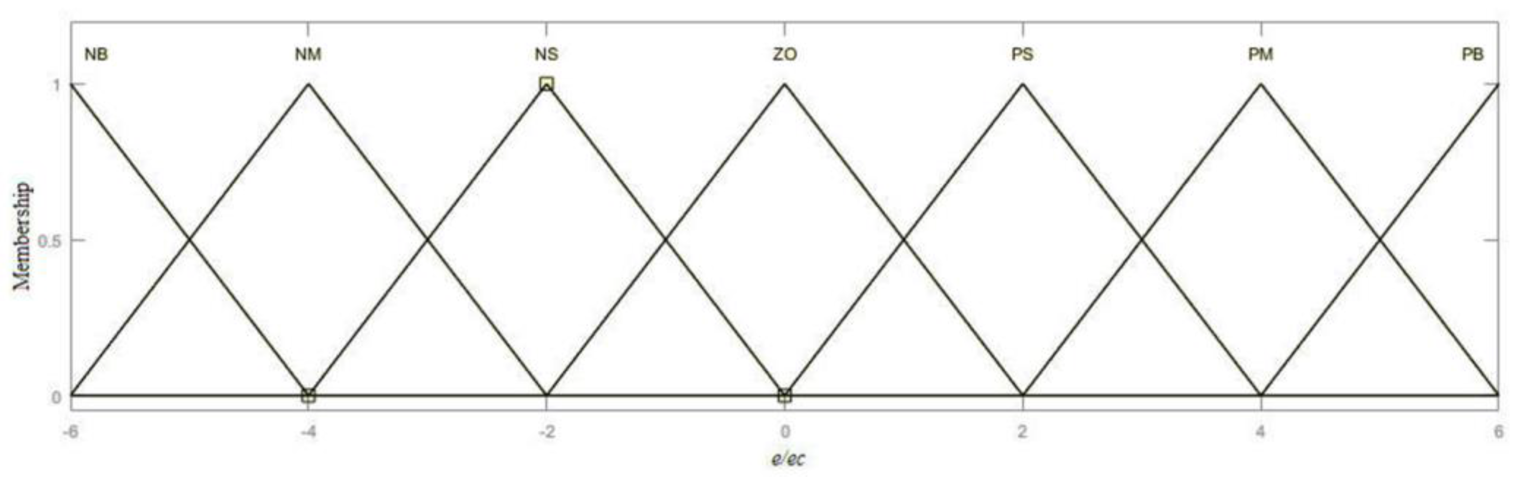
3.2.2. Fuzzification of Input and Output Variables

The basic domain of the input e was [−20°, 20°], which was converted to radians as [−0.35, 0.35]. The basic domain of the input ec was [−40°, 40°], which was converted to radians as [−0.35, 0.35]. The fuzzy domains of e and ec were both [–6, 6], so the quantization factor k_e of e was 17.14 and the quantization factor k_ec of ec was 8.57. We used seven linguistic values for the fuzzy variables, namely negative big (NB), negative medium (NM), negative small (NS), zero (ZO), positive small (PS), positive medium (PM), and positive big (PB). The triangle membership functions were used because they are suitable for online adjustment, as shown in Figure 7.

Increasing the proportional coefficient Kp can speed up the system response, but if it is too large, the system will become unstable. Likewise, a too large K_d may lead to instability. Therefore, the basic domains of ΔKp, ΔK_i, and ΔK_d were all set as [−3, 3], and the quantization levels were {−3, −2, −1, 0, 1, 2, 3}. The corresponding membership functions are shown in Figure 8.

3.2.3. Fuzzy Rules

Establishing the fuzzy rules required the full consideration of the characteristics of boom control. When e and ec are large, indicating a significant deviation between the current and target angle values, ΔKp and ΔK_i should be increased to reduce the angle difference, and an appropriate value should be selected for ΔK_d [29,30,31]. Comprehensively taking into account the influence of K_p, K_i, and K_d on the dynamic and static performance of the system, a fuzzy rule table was determined (

Table 1. Fuzzy rules of ΔKp, ΔK_i, and ΔK_d.

e	ec
	NB	NM	NS	ZO	PS	PM	PB
NB	PB/NB/PS	PM/PB/PS	ZO/NM/NM	PM/NM/NB	NB/NS/NM	NB/ZO/NB	NS/ZO/PS
NM	PB/NB/NS	PB/PB/NS	PM/NM/NS	PS/NS/NM	PS/NS/NM	ZO/ZO/NS	ZO/ZO/ZO
NS	PB/NS/ZO	PM/NB/NS	PS/NS/NM	ZO/NS/ZO	ZO/ZO/NS	NS/PS/NS	NS/PS/PS
ZO	PM/NM/ZO	PS/NB/NS	PS/NS/NS	ZO/ZO/ZO	ZO/ZO/ZO	PS/NS/ZO	ZO/ZO/NS
PS	PS/NM/ZO	PS/NS/ZO	ZO/ZO/NS	NM/ZO/ZO	NS/PS/NM	NM/PM/ZO	NB/PM/ZO
PM	PS/ZO/NB	PS/ZO/NS	PM/ZO/ZO	ZO/PS/ZO	NS/PM/PM	NM/PB/PS	NB/PB/PB
PB	ZO/ZO/PB	ZO/ZO/PM	NS/PS/ZO	NS/PS/PM	NM/PM/PS	NB/PB/PB	NB/PB/PB

), which included a total of 147 fuzzy rules.

3.2.4. Parameter Tuning

Based on the membership functions and fuzzy rules, fuzzy inference was performed using the Mamdani method, and defuzzification was carried out using the centroid method. The fuzzy process is shown in Figure 9.

As the fuzzy domain of the ΔKp, ΔK_i, and ΔK_d outputs was [−3, 3], while their physical domains were [−6, 6], [−0.15, 0.15], and [−1.5, 1.5], respectively, the proportionality factors were k_up = 2, k_ui = 0.05, and k_ud = 0.5. Therefore, the PID control parameters were

$$\left\{\begin{array}{c}{K}_p=K_{p0}+k_{up}\Delta K_p\\ K_i=K_{i0}+k_{ui}\Delta K_i\\ K_d=K_{d0}+k_{ud}\Delta K_d\end{array}\right.,$$

(13)

where K_p0, K_i0, and K_d0 are the initial parameters for PID control.

3.3. Particle Swarm Optimization (PSO) Algorithm and Simulation

3.3.1. PSO Algorithm

The outputs of the fuzzy PID controller were ΔKp, ΔK_i, and ΔK_d. The initial values of the PID control parameters needed to be selected by experience, and the size of the initial values had a significant impact on the system performance. Therefore, the PSO algorithm was used to optimize the initial parameters.

The global optimization problem can be expressed as

$$\left\{\begin{array}{c}\min \sigma =f(Z)\\ Z=\left\{Z_1,Z_2,\cdots ,Z_n\right\}\\ Z_i=\left\{z_{i1},z_{i2},\cdots ,z_{im}\right\}\end{array}\right.,$$

(14)

where Z represents a particle swarm formed by n particles, and Z_i represents the position of each particle.

The update equations for the flight speed and position of particles are

$$\left\{\begin{array}{l}{v}_{id}(t+1)=v_{id}(t)+c_1{r}_1(p_{id}(t)-x_{id}(t))+c_2{r}_2\left(p_{gd}(t)-x_{id}(t)\right)\\ x_{id}(t+1)=x_{id}(t)+v_{id}(t+1)\end{array}\right.,$$

(15)

where x_id represents the d-th value in the position of the i-th particle in the particle swarm; v_id represents the d-th parameter value in the speed of the i-th particle; p_id represents the d-th value in the best position experienced by the i-th particle; p_gd represents the d-th value in the best position experienced by all particles in the swarm; c₁ represents the cognitive learning factor, which controls the acceleration constant of particles flying towards their own best position; c₂ represents the social learning factor, which controls the acceleration constant of particles flying towards the global best position; and r₁ and r₂ are independent random numbers between 0 and 1.

In the process of seeking the optimal solution, the selection of flight speed is related to the function of the algorithm. An excessively high speed may cause the particle to fly past the optimal position, while a speed that is too low may easily trap the particle in a local optimum. Therefore, the speed was adjusted by introducing an inertia weight, and Equation (15) was modified as follows:

$$\left\{\begin{array}{l}{v}_{id}(t+1)=\omega v_{id}(t)+c_1{r}_1(p_{id}(t)-x_{id}(t))+c_2{r}_2\left(p_{gd}(t)-x_{id}(t)\right)\\ x_{id}(t+1)=x_{id}(t)+v_{id}(t+1)\end{array}\right.,$$

(16)

where ω represents the inertia weight.

To improve the global search ability in the early stage, ω is usually set to 0.9. To enhance the local search ability in the later stage, ω is usually set to 0.4. During the search process, the value of ω decreases linearly over time. The calculation formula is

$$\omega ={\omega }_s+({\omega }_T-{\omega }_s)t/T_{\max },$$

(17)

where ω_s represents the initial inertia weight; ω_T represents the final inertia weight; T_max represents the maximum number of iterations; and t represents the iteration durations.

To improve the performance of the PSO algorithm, time-varying parameters were used to dynamically adjust the values of c₁ and c₂.

The adjustment method for c₁ was

$$c_1(t)=(c_{1T}-c_{1s})t/T_{\max }+c_{1s},$$

(18)

where c_1s represents the initial cognitive learning factor, and c_1T represents the final cognitive learning factor.

The adjustment method for c₂ was

$$c_2(t)=(c_{2T}-c_{2s})t/T_{\max }+c_{2s},$$

(19)

where c_2s represents the initial social learning factor, and c_2T represents the final social learning factor.

The PSO algorithm flowchart is shown in Figure 10.

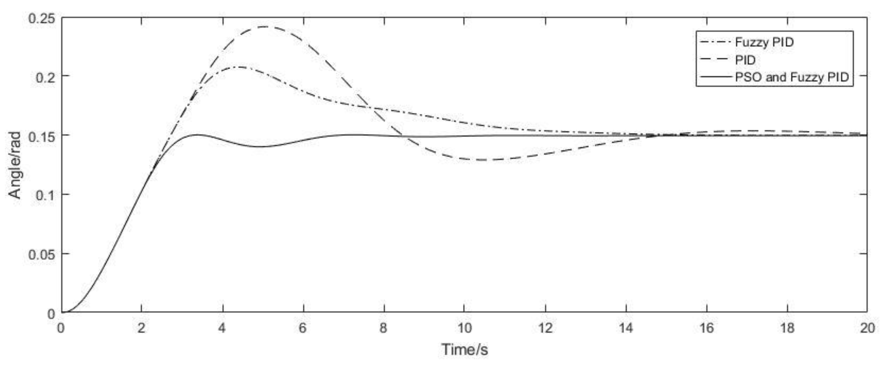
3.3.2. Simulation Analysis

To verify the effectiveness of using the PSO algorithm to optimize PID control parameters, a simulation was conducted in Simulink R2016a software. The step response analysis of the inclination angle of the boom was carried out to validate the angle tracking effect of the controller. Using a boom inclination angle of 0.15 rad as the control target, a fuzzy model was established through the built-in fuzzy logic toolbox of Matlab R2016a. The fuzzy logic file was loaded into the fuzzy logic controller model. The values of the parameters in the transfer function of the active suspension were: l₁ = 0.45 m, l₂ = 0.25 m, l₃ = 0.2 m, m = 49 kg, I = 93 kg·m², cl_d² = 200 Nms·rad⁻¹, kl_s² = 0, and g = 9.8 m/s². Taking into account the speed limit of the electric linear actuator (12 mm/s), the displacement saturation limit, the time delay of 0.1 s between the forward and reverse directions of the motor, and the system delay of 0.1 s, the simulation model shown in Figure 11 was established.

The parameters for conventional PID control were K_p = 3.3, K_i = 5.5, and K_d = 3.0, and the parameters for fuzzy PID control were K_p = 15, K_i = 5, K_d = 8, k_up = 2, k_ui = 0.05, k_ud = 0.5, k_e = 17.14, and k_ec = 8.57. The parameters for PSO fuzzy PID control were n = 50, Dim = 3, ω_s =0.9, ω_T =0.4, c_1s = 2.0, c_1T = 0.5, c_2s = 0.5, c_2T = 2.0, U_b = 10, L_b = 0, and t = 30. The objective function used an integral performance index. The PID parameters optimized using PSO were K_p = 10, K_i = 0.06, and K_d = 4.27.

The step response of the above three methods is shown in Figure 12.

According to Figure 12 the overshoot of the system was 56.80% and the settling time was 17.90 s when using conventional PID control. The overshoot was 38.33% and the settling time was 12.30 s when using fuzzy PID control. The overshoot was 1.53% and the settling time was 5.4 s when using PSO-based fuzzy PID control. The performance of the boom control system was optimized using PSO-based fuzzy PID control, which not only reduced the overshoot but also reduced the settling time. The control effect and robustness of the system were better.

4. Experiments and Results

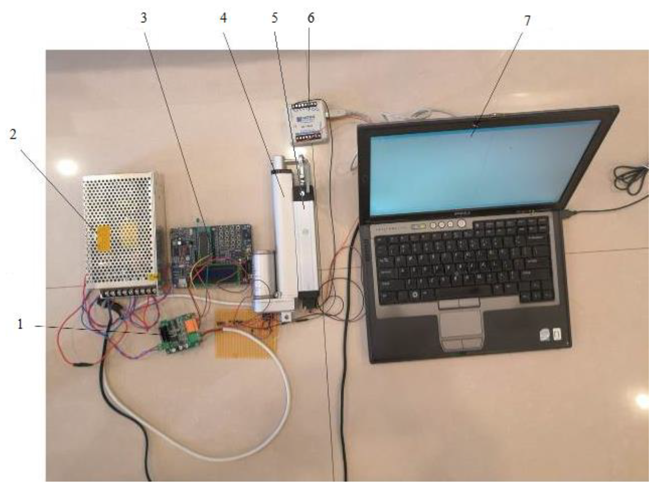
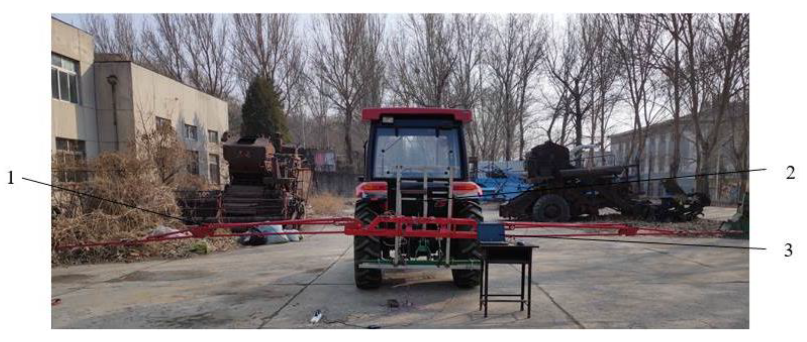
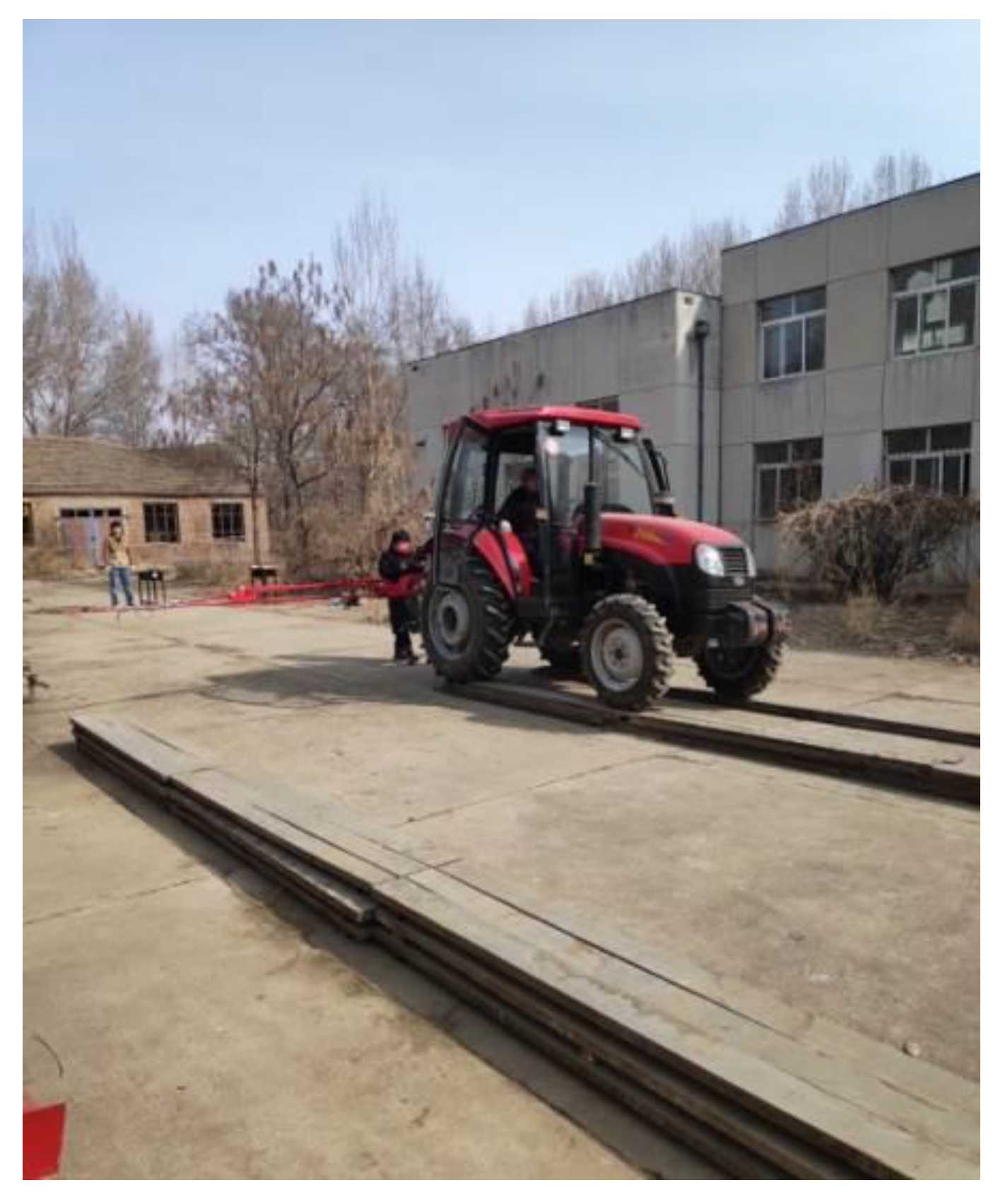
4.1. Experimental Device

The experimental device comprised a spray boom, suspension system, data acquisition system, and control system, as shown in Figure 13.The spray boom was a purchased three-stage foldable boom, with a middle spray frame length of 2 m and two side spray arms on the left and right sides, both 3.5 m long. The mass of the spray boom was measured by a scale and was found to be 49 kg. The 3D model of the spray boom was established using Pro/Engineering, and the moment of inertia of the boom around its center of mass was calculated to be 93 kg·m². The first pendulum rod of the suspension system was 0.45 m long, and the second pendulum rod was 0.25 m long. The damping coefficient of the damper was 1875 N·s/m. The stiffness coefficient of the spring was 730 N/m.

4.2. Experimental Method

There are three methods for testing the stability of a spray boom: a field test, a simulation test, and a runway test. Field tests take place in a real field environment, but it is difficult to control the ground undulation, and this method cannot provide the required excitation signal. Simulation tests require special simulators for generating simulation stimuli, such as sine vibration or random signals, to force the stationary sprayer to move in different directions, and the test conditions are demanding. Therefore, runway tests were used in this study, placing obstacles on the runway and using a bumpy runway to generate low-frequency or high-frequency signals in order to simulate field operating conditions in a reproducible manner.

The commonly used types of stimuli for testing the stability of spray booms include step signals, sine signals, and pulse signals. Since the input represented by the step signal is relatively harsh and has strong representativeness, if the performance indicators of the system can meet the requirements under step signal excitation, the performance will also meet the requirements under other types of signal excitation. Therefore, in this study, a step signal was used as an input to excite the tractor wheels in order to test the stability of the spray boom [4]. The test pavement was cement ground, and in order to facilitate disassembly, wooden boards of a certain height were placed down to simulate ground slopes. A cement pavement is more demanding than a soil environment and could also ensure the integrity of the signals required for the experiment [32].

In order to test the performance of the active suspension system on sloping terrain, an experimental area was designed to simulate field sloping terrain, as shown in Figure 14. The simulated slope represented a step excitation for the suspension system. If its angle was too small, the excitation would not be sufficient, and if it was too large, nonlinear factors could easily be introduced. Referring to the relevant literature and considering experimental conditions, the angle was set to be 1.5°. With the known spray boom length of 9 m and tractor wheelbase of 1.4 m, the corresponding dimensions in the figure could be calculated: h₁ was 0.099 m, h₂ was 0.136 m, h₃ was 0.235 m, l₁ was 1.4 m, and l₂ was 3.1 m. The experimental process and data acquisition are shown in Figure 15 and Figure 16.

Two ultrasonic sensors were mounted on the left and right tips of the boom, as shown in Figure 17. The angle between the boom and the ground could be calculated as

$$\theta =\arcsin (\frac{H_1-H_2}{L}),$$

(20)

where H₁ represents the measured value of the right sensor; H₂ represents the measured value of the left sensor; and L represents the installation distance between the two sensors.

When an ultrasonic sensor is used, it emits a conical beam of ultrasonic waves. The ultrasonic waves within the beam angle can generate valid echoes. Since the ultrasonic sensor calculates distance based on the timing of the echo, the measured value represents the distance between the sensor and the nearest point. As long as the ground slope angle is not greater than the beam angle of the sensor, the vertical distance from the sensor to the ground can be measured. In field conditions, air temperature, humidity, and wind velocity can influence the performance of ultrasonic sensors. In our study, the ultrasonic sensor had a built-in temperature senor to compensate for the effect of temperature fluctuation. The abnormal values caused by other factors could be eliminated through filter algorithms.

The inclination angle of the spray boom could be calculated by the angle θ and the inclination angle of the vehicle body. The inclination angle of the vehicle body could be measured by the angle sensor installed on the sprayer frame.

4.3. Results and Discussion

The inclination angle of the vehicle body is easily influenced by factors such as ground excitation, tire excitation, and engine vibration. In order to reduce the influence of interference on the results, data with an absolute difference greater than 1.0° from the previous sampling value were first removed. Then, a five-point third-order smoothing method was used to process the inclination angle of the vehicle body. The inclination angle of the vehicle body and the boom is shown in Figure 18.

From Figure 18, it can be found that when the sprayer was traveling on the flat ground, the range of the inclination angle of the vehicle body was −0.35~0.40°, while the inclination angle of the boom remained at −0.13~0.17°. When the sprayer drove up the slope from the flat ground, there was a sudden change in the inclination angle of the vehicle body. The control system could make the inclination angle of the boom follow the change in the inclination angle of the vehicle body, so the boom could remain parallel to the ground. The response time was about 5 s. When the sprayer was on the slope, the range of the inclination angle of the vehicle body was 1.15~1.89°, while the inclination angle of the boom remained within the range of 1.42~1.60° after balancing. The experimental results showed that the control system for the active suspension system designed in this paper could automatically adjust the inclination angle of the boom according to the change in the slope angle and meet the requirements of spray operation.

At present, there are no clear requirements regarding the response time of a control system during the field operation of a boom sprayer. Ref. [21] reported that the response time of the boom inclination angle was approximately 4 s when using adaptive fuzzy sliding mode control. Ref. [22] reported that it took 5.71 s for the boom roll control system to bring the boom to the equilibrium position. Referring to the above research conclusions, the response time of our study could meet the actual control requirements. In future research, we will focus on shortening the response time by utilizing a linear actuator with a higher power and further optimizing the control algorithm.

5. Conclusions

An active suspension control system based on a CAN bus was constructed, consisting of a main control node, two distance measurement nodes, a vehicle inclination detection node, and an execution node. The transfer functions of the active suspension and electric linear actuator were established. In order to improve the performance of the control system, the initial parameters of the fuzzy PID controller were optimized using the PSO algorithm. The fuzzy controller was constructed based on the deviation and deviation rate of the boom inclination angle, and the fuzzy control algorithm was used to optimize the increments in the PID control parameters. The simulation results showed that compared to the conventional PID controller and fuzzy PID controller, the PSO-based fuzzy PID controller exhibited a reduced overshoot and decreased settling time, effectively improving the control performance. The results of the simulated slope test showed that the boom could quickly follow changes in the ground slope angle, and the fluctuation range of the inclination angle of the boom was significantly lower than that of the vehicle body. This indicated that the control system for double-pendulum active spray boom suspension effectively isolated high-frequency disturbances and followed low-frequency ground undulations, meeting the operational requirements.

References

1. He, X. Research progress and developmental recommendations on precision spraying technology and equipment in China. Smart Agric. 2020, 2, 133–146. [Google Scholar]
2. He, X. Research and development of efficient plant protection equipment and precision spraying technology in China: A review. J. Plant Protec. 2022, 1, 389–397. [Google Scholar]
3. Qiu, B.; Yan, R.; Ma, J.; Guan, X.; Ou, M. Research progress analysis of variable rate sprayer technology. Trans. CSAM 2015, 46, 59–72. [Google Scholar]
4. Jeon, H.Y.; Womac, A.R.; Gunn, J. Sprayer boom dynamic effects on application uniformity. Trans. CSAE 2004, 47, 647–658. [Google Scholar]
5. Jia, W.; Zhang, L.; Yan, M.; Xue, X. Current situation and development trend of boom sprayer. J. Chin. Agric. Mech. 2013, 34, 19–22. [Google Scholar]
6. Jeon, H.Y.; Womac, A.R.; Wilkerson, J.B.; Hart, W.E. Sprayer boom instrumentation for field use. Trans. ASAE 2004, 47, 659–666. [Google Scholar] [CrossRef]
7. Balsari, P.; Gil, E.; Marucco, P. Field-crop-sprayer potential drift measured using test bench. Biosyst. Eng. 2017, 154, 3–13. [Google Scholar] [CrossRef]
8. Ramon, H.; Baerdemaeker, J.D. Spray boom motions and spray distribution: Part l-Derivation of a mathematical relation. J. Agric. Eng. Res. 1997, 66, 23–29. [Google Scholar] [CrossRef]
9. Ramon, H.; Missotten, B.; Baerdemaeker, J.D. Spray boom motions and spray distribution: Part 2-experimental validation of the mathematical relation and simulation results. J. Agric. Eng. Res. 1997, 66, 31–39. [Google Scholar] [CrossRef]
10. Cui, L.; Xue, X.; Le, F.; Mao, H.; Ding, S. Design and experiment of electro hydraulic active suspension for controlling the rolling motion of spray boom. Int. J. Agric. Biol. Eng. 2019, 12, 72–81. [Google Scholar] [CrossRef]
11. Deprez, K.; Anthonis, J.; Ramon, H. System for vertical boom corrections on hilly fields. J. Sound Vib. 2003, 266, 613–624. [Google Scholar] [CrossRef]
12. Tahmasebi, M.; Rahman, R.A.; Mailah, M.; Gohari, M. Active force control applied to spray boom structure. Appl. Mech. Mater. J. 2013, 315, 616–620. [Google Scholar] [CrossRef]
13. Deprez, K.; Anthonis, J.; Ramon, H. Development of a slow active suspension for stabilizing the roll of spray booms: Part 1—Hybrid modelling. Biosyst. Eng. 2002, 81, 185–191. [Google Scholar] [CrossRef]
14. Deprez, K.; Anthonis, J.; Ramon, H. Development of a slow active suspension for stabilizing the roll of spray booms: Part 2: Controller design. Biosyst. Eng. 2002, 81, 273–279. [Google Scholar] [CrossRef]
15. Anthonis, J.; Audenaert, J.; Ramon, H. Design optimization for the vertical suspension of a crop sprayer boom. Biosyst. Eng. 2005, 90, 153–160. [Google Scholar] [CrossRef]
16. O’Sullivan, J.A. Simulation of the behavior of a spray boom with an active and passive pendulum suspension. J. Agric. Eng. Res. 1986, 35, 157–173. [Google Scholar] [CrossRef]
17. O’Sullivan, J.A. Verification of passive and active versions of a mathematical model of a pendulum spray boom suspension. J. Agric. Eng. Res. 1988, 40, 89–101. [Google Scholar] [CrossRef]
18. Frost, A.R. Simulation of an active spray boom suspension. J. Agric. Eng. Res. 1984, 30, 313–325. [Google Scholar] [CrossRef]
19. Cui, L.; Xue, X.; Ding, S.; Gu, W.; Chen, C.; Le, F. Modeling and simulation of dynamic behavior of large spray boom with active and passive pendulum suspension. Trans. CSAM 2017, 48, 82–90. [Google Scholar]
20. Cui, L.; Xue, X.; Ding, S.; Qiao, B.; Le, F. Analysis and test of dynamic characteristics of large spraying boom and pendulum suspension damping system. Trans. CSAE 2017, 33, 69–76. [Google Scholar]
21. Xue, T.; Li, W.; Du, Y.; Mao, E.; Wen, H. Adaptive fuzzy sliding mode control of spray boom active suspension for large high clearance sprayer. Trans. CSAE 2018, 34, 47–56. [Google Scholar]
22. Cui, L.; Xue, X.; Ding, S.; Le, F. Development of a DSP-based electronic control system for the active spray boom suspension. Comput. Electron. Agric. 2019, 166, 105024. [Google Scholar] [CrossRef]
23. Cui, L.; Xue, X.; Le, F.; Ding, S. Adaptive robust control of active and passive pendulum suspension for large boom sprayer. Trans. CSAM 2020, 51, 130–141. [Google Scholar]
24. Chen, W.; Qiu, B.; Yang, N. Spray boom position control system based on ultrasonic sensors. J. Agric. Mechan. Res. 2013, 3, 84–87. [Google Scholar]
25. Wang, S.; Zhao, C.; Wang, X. Design and experiments on boom height adjusting system. J. Agric. Mechan. Res. 2014, 8, 161–164. [Google Scholar]
26. Chang, C. Remote Measuring and Controlling System Design of Six-DOF Parallel Platform. Master’s Thesis, Dalian University of Technology, Dalian, China, 2015. [Google Scholar]
27. Yang, J. The Research on 6-DOF Parallel Micro-Positioning Platform Control System Based on the Embedded System. Master’s Thesis, The First Academy of China Aerospace Science and Technology Corporation, Beijing, China, 2017. [Google Scholar]
28. Xue, T.; Liu, Z.; Huo, J.; Wang, H.; Li, X.; Jiang, S. Design of mechanical automatic control system based on integral discrete PID algorithm. J. Xinyang Normal Univ. 2020, 33, 138–143. [Google Scholar]
29. Miao, W.; Zhou, Z.; Xuan, J.; Cheng, D.; Cao, N. Design and simulation of ball balancing robot controller based on fuzzy PID. Transducer Microsyst. Technol. 2021, 40, 66–70. [Google Scholar]
30. Shi, C.; Zhang, Y. Research on speed control of hydraulic drive spindle based on fuzzy adaptive PID controller. Chinese J. Constr. Mach. 2020, 18, 516–520. [Google Scholar]
31. Ma, Y.; Ding, H.; Mu, H.; Chen, H. Liquid cooling strategy of power battery based on fuzzy PID algorithm. Control Theoryand Appl. 2021, 38, 549–560. [Google Scholar]
32. Jeon, H.Y.; Zhu, H.; Derksen, R.; Ozkan, E.; Krause, C. Evaluation of ultrasonic sensor for variable-rate spray applications. Comput. Electron. Agric. 2011, 75, 213–221. [Google Scholar] [CrossRef]
Figure 1. Structure of the double-pendulum suspension system: 1—ground, 2—frame, 3—boom, 4—actuator, 5—second pendulum rod, 6—damper, 7—spring, 8—first pendulum rod, 9—ranging sensor.
Agriculture 13 01660 g001
Figure 2. Equipment for determining the parameters of the transfer function: 1—river, 2—power supply, 3—single-chip microcomputer, 4—electric linear actuator, 5—linear displacement sensor, 6—data acquisition device, 7—computer.
Agriculture 13 01660 g002
Figure 3. Step response of the actuator piston rod velocity.
Agriculture 13 01660 g003
Figure 4. Overall structure of the control system.
Agriculture 13 01660 g004
Figure 5. Circuits for distance measurement and actuator drive: 1—first CAN bus connector, 2—terminal resistor, 3—first CAN bus conversion module, 4—first microcomputer system, 5—ultrasonic sensor, 6—motor drive module, 7—second microcomputer system, 8—second CAN bus conversion module, 9—electric linear actuator, 10—second CAN bus connector.
Agriculture 13 01660 g005
Figure 6. Structure of the fuzzy PID control system.
Agriculture 13 01660 g006
Figure 7. Membership functions of input e and ec.
Agriculture 13 01660 g007
Figure 8. Membership functions of ΔKp, ΔKi, and ΔKd.
Agriculture 13 01660 g008
Figure 9. Diagram of fuzzy inference.
Agriculture 13 01660 g009
Figure 10. PSO algorithm flowchart. Note: n represents the number of particles, Dim represents the dimensionality of the particles, Ub represents the maximum value of the search range, Lb represents the minimum value of the search range, fid represents the optimal fitness value of an individual particle, fgd represents the global optimal fitness value, fmin represents the minimum fitness value, and fzi represents the fitness value of the i-th particle.
Agriculture 13 01660 g010
Figure 11. Simulation model of the PSO-based fuzzy PID boom control system.
Agriculture 13 01660 g011
Figure 12. Step response of the inclination angle of the boom for different control strategies.
Agriculture 13 01660 g012
Figure 13. Experimental device: 1—spray boom, 2—suspension, 3—data acquisition system.
Agriculture 13 01660 g013
Figure 14. Schematic diagram of the simulated slope.
Agriculture 13 01660 g014
Figure 15. Experimental process.
Agriculture 13 01660 g015
Figure 16. Data acquisition.
Agriculture 13 01660 g016
Figure 17. Layout of the ultrasonic sensors on the boom: 1—ground, 2—right ultrasonic sensor, 3—boom, 4—left ultrasonic sensor.
Agriculture 13 01660 g017
Figure 18. Test curves of the inclination angle of the vehicle body and the boom.
Agriculture 13 01660 g018