Article

Forecasting Pesticide Use on Golf Courses by Integration of Deep Learning and Decision Tree Techniques

1
Centre de Recherche et d’Innovation sur les Végétaux, Département de Phytologie, Université Laval, Québec, QC G1V 0A6, Canada
2
Department of Soils and Agri-Food Engineering, Université Laval, Québec, QC G1V 0A6, Canada
3
Department of Civil Engineering, University of Ottawa, 161 Louis Pasteur Private, Ottawa, ON K1N 6N5, Canada
*
Author to whom correspondence should be addressed.
Agriculture 2023, 13(6), 1163; https://doi.org/10.3390/agriculture13061163
Submission received: 4 May 2023 / Revised: 27 May 2023 / Accepted: 28 May 2023 / Published: 30 May 2023
(This article belongs to the Section Digital Agriculture)

Abstract

:
In the current study, a new hybrid machine learning (ML)-based model was developed by integrating a convolution neural network (CNN) with a random forest (RF) to forecast pesticide use on golf courses in Québec, Canada. Three main groups of independent variables were used to estimate pesticide use on golf courses, expressed as actual active ingredient rate (AAIR): (i) coordinates (i.e., longitude and latitude of the golf course), (ii) characteristics of the golf courses (i.e., pesticide type and the number of holes), and (iii) meteorological variables (i.e., total precipitation, P, and average temperature, T). The meteorological variables were collected from the Google Earth Engine by developing a JavaScript-based Code. On the basis of the different periods of total precipitation and average temperature, four different scenarios were defined. A data bank with more than 40,000 samples was used to calibrate and validate the developed model such that 70% of all samples were randomly selected to calibrate the model, while the remainder of the samples (i.e., 30%) that did not have any role in calibration were employed to validate the model’s generalizability. A comparison of different scenarios indicated that the model that considered the longitude and latitude of the golf course, pesticide type, and the number of holes in golf courses as well as total precipitation and average temperature from May to November as inputs (R = 0.997; NSE = 0.997; RMSE = 0.046; MAE = 0.026; NRMSE = 0.454; and PBIAS (%) = −0.443) outperformed the other models. Moreover, the sensitivity analysis result indicated that the total precipitation was the most critical variable in AAIR forecasting, while the average temperature, pesticide types, and the number of holes were ranked second to fourth, respectively.

1. Introduction

Golf courses are high-maintenance environments that often require the use of inputs such as pesticides to maintain their playing surfaces. While golf courses can provide several environmental benefits, this pesticide use has led to criticism from the public and sometimes to regulations from governing authorities. For example, since 2003, golf managers in the Québec province of Canada have been required to submit a “Pesticide Reduction Plan” (PRP), signed by a licensed agronomist, to the Ministry of the Environment and the Fight Against Climate Change (MELCC: Ministère de l’Environnement et de la Lutte aux Changements Climatiques) every three years. These PRPs must contain six different items [1], including quantities of pesticides applied for each category (fungicides, herbicides, insecticides, etc.) on the corresponding treated area, methods implemented to prevent pesticide migration outside the course, and alternative approaches for monitoring and controlling pests without pesticides. Finally, these PRPs should also include objectives in reducing each pesticide category for the next three years and the methods that will be implemented to achieve these objectives. Since insect and disease incidence is highly dependent on weather conditions and can vary significantly from year to year, it can be difficult to predict pesticide use and, thus, set realistic objectives in pesticide reductions for golf course managers. In this context, the use of machine learning (ML) could be helpful for golf course managers and regulatory authorities to better refine the process through which the objectives in pesticide reductions are set.
ML has been previously used to predict pesticide behavior as well as its impact on human health and the environment. For example, Kobayashi et al. [2] developed a model to predict the soil adsorption coefficient (Koc) of pesticides by comparing three different algorithms (gradient boosting decision tree, multiple linear regression, and support vector machine). Vaz et al. [3] were able to develop three new molecules effective against plant diseases by using ML on a training set of molecules with known activity. In a review study on the use of prediction models for pesticide use, Gilbert and Edwin [4] proposed different models based on deep learning to predict pesticide use on the basis of the occurrence of pests or past pesticide use. Different ML techniques have also been used to identify pesticide residues on fruits and vegetables [5,6] and to evaluate the toxicity of pesticides against non-target organisms [7,8].
In a previous study [9], we used the database of pesticide applications compiled by the MELCC from 2003 to 2018 to develop a machine learning algorithm that can reliably predict pesticide use on golf courses in Québec. This algorithm relied on a hybrid approach combining a tree-based method (random forest—RF) and a non-tree-based method (support vector machine—SVM) followed by an optimization phase (grasshopper optimization algorithm—GOA). Using golf course characteristics, such as its ID and localization (region), the number of holes, and the total treated area, the RF-SVM-GOA algorithm was able to reliably predict pesticide use on golf courses. However, this model had some drawbacks, as it relied entirely on golf course characteristics and did not consider other factors affecting pest development, such as weather conditions. Furthermore, the complexity of the model required very high computer processing power, which limited its application to only 14,000 samples out of the more than 40,000 samples available in the database.
Thus, the main objective of the current study was to develop a new hybrid computer program for predicting golf pesticide use that can (i) analyze the applications of pesticides on golf courses in the province of Québec, Canada, (ii) assess the importance of different types of parameters on the use of pesticides on golf courses, and (iii) predict future pesticide use, which is critical for golf management to meet pesticide reduction targets.

2. Materials and Methods

2.1. Study Area and Data Collection

Since the adoption of the Pesticide Management Code in 2003, the MELCC has compiled a database of all golf course pesticide applications in the province of Québec. This database includes various information, such as the identification of the golf courses, types of applied pesticides, applied rates, and treated area for 380 golf courses during the 2003–2017 period. The location of all these golf courses is provided in Figure 1. Most golf courses are located in areas with high population density in the south of the province, with some located in residential areas less densely populated, such as the southwest and southeast areas of the province.
The developed ML model includes three types of input variables: (i) characteristics of the golf courses, such as the number of holes (NH) and pesticide type (PT), (ii) coordinates of each golf course, such as longitude (X) and latitude (Y), and (iii) meteorological variables, including total precipitation (P) and average temperature (T). NH, PT, X, and Y were obtained from the MELCC golf pesticide database, while P and T were collected using the Google Earth Engine (GEE).
The output of the model is the actual active ingredient rate (AAIR) compiled from the golf pesticide database. It represents the total active ingredient applied over a specific area in kg 100 m−2 and is defined as follows:
A A I R = A I T T r e a t e d A r e a = Q × C T r e a t e d A r e a
where AIT is the actual ingredient total (kg), Q is the pesticide quantity (kg), C is the concentration of the active ingredient in the applied pesticide (%), and the Treated Area is expressed in m2. For simplicity, pesticide density was considered to be equivalent to 1 kg L−1, allowing for easy conversion of liters into kg for pesticides sold in a liquid form.

2.1.1. Meteorological Dataset

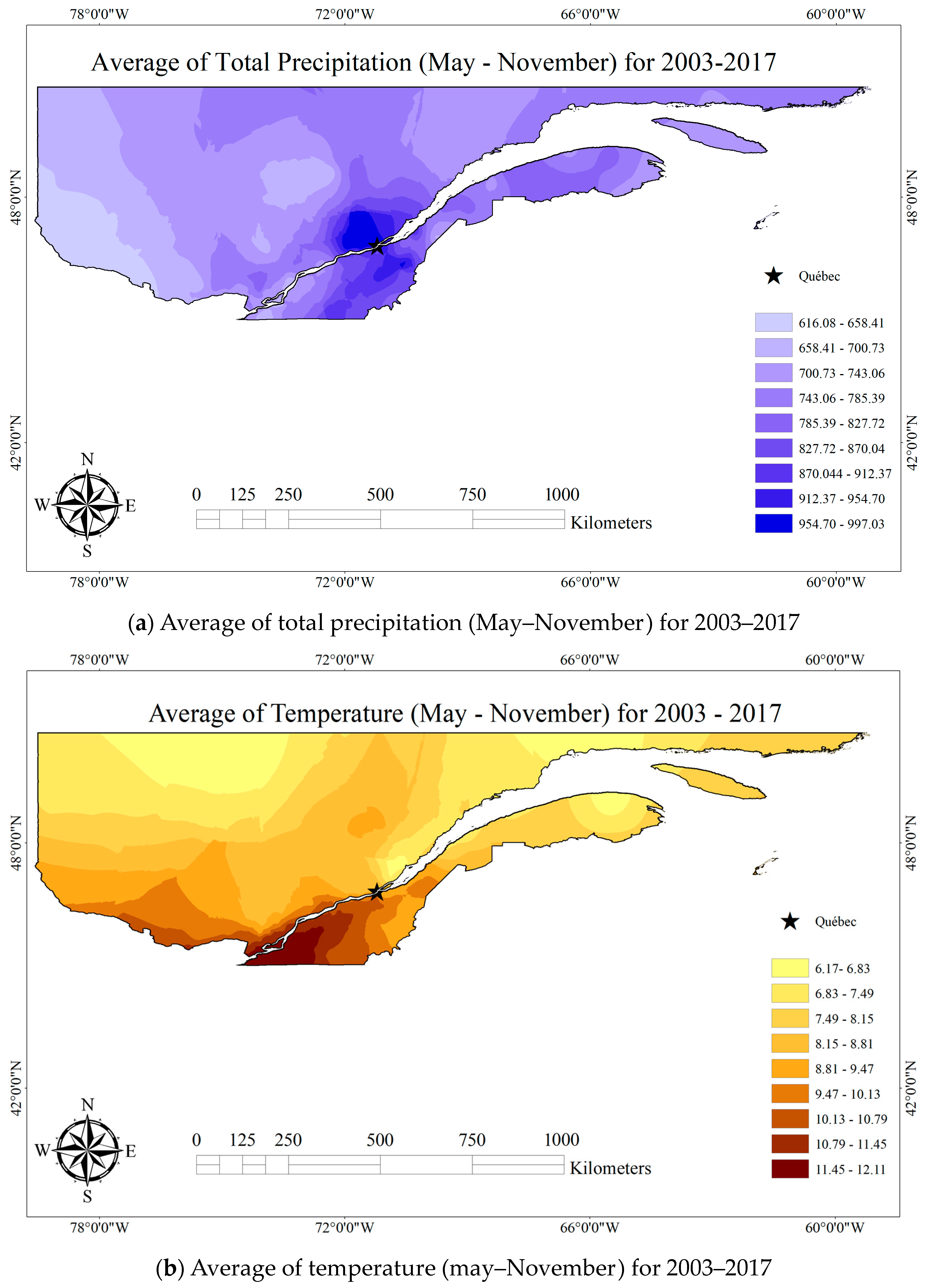
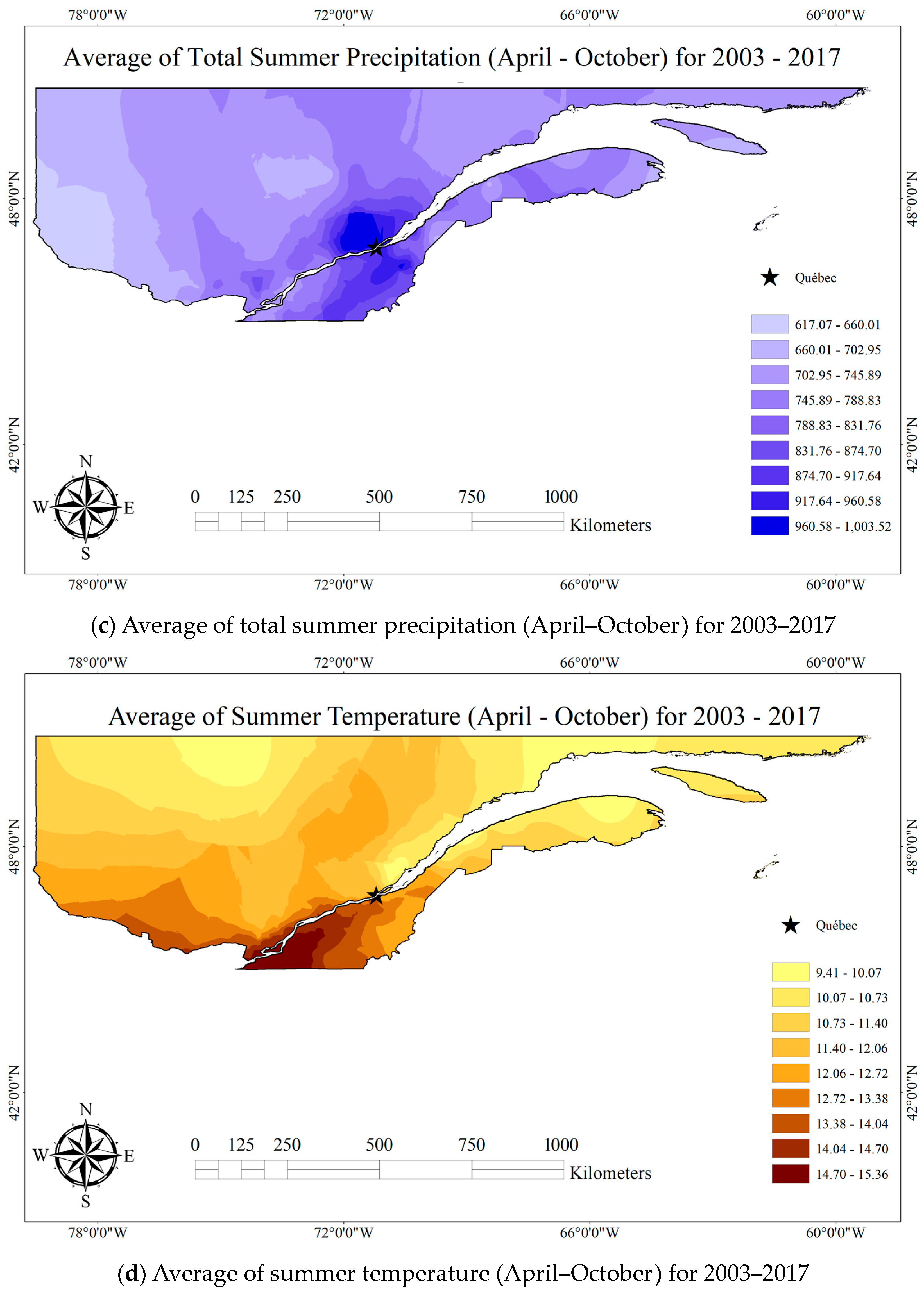
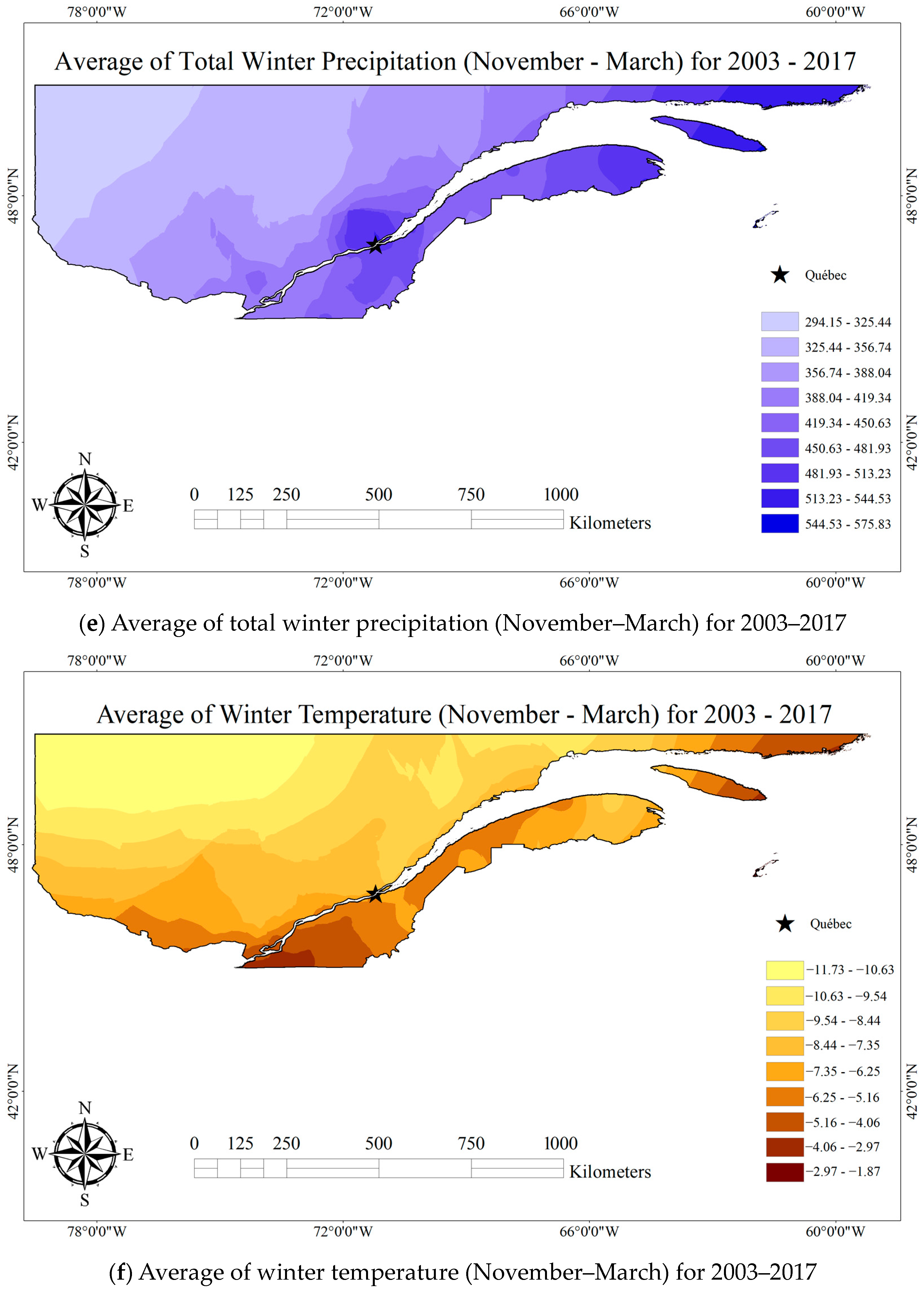
The Google Earth Engine (GEE) was employed to collect the meteorological dataset. However, although GEE supports large-scale computing, it requires specialized expertise [10]. Therefore, a JavaScript code was developed to preprocess gathered information from ground-based observations and satellite images data products in GEE. Total precipitation and average temperature were compiled from 2003 to 2017 for three different periods. The first period, from May to November, aligns with the typical golf season in southern Québec and is denoted as PSeason (precipitation) and TSeason (temperature). The second period, spanning from April to October, represents the summer months characterized by minimal snowfall and frosts and is referred to as PSummer and TSummer. The third period encompasses the months from November to March, known as the winter months, characterized by the presence of snow and consistently sub-zero temperatures. This period is denoted as PWinter (precipitation) and TWinter (temperature). Although plant growth is typically limited during the winter months, the survival of pests, including insects and fungal diseases, can be influenced by temperature and snow cover, thus impacting the subsequent growing season’s requirement for fungicides and insecticides. Figure 2 shows the distribution of the meteorological variables (total precipitation and average temperature) for the three periods considered. Since no golf courses are located in the central and northern regions of Québec province, the provided maps cover only the areas where golf courses are located to create more precise maps showing the differences in meteorological parameters among golf courses.
The total precipitation from May to November (PSeason) throughout 15 years shows that the difference between the minimum and maximum total precipitation is more than 392 mm (Figure 2a). The minimum PSeason occurs in the southwest of Québec province, while the maximum occurs in Québec City. Similarly, the difference between the minimum and maximum of PSummer is significant (Figure 2b). Compared with the maximum PSummer, the minimum is far from the south. In addition, the maximum PSummer is almost in the same area as the maximum PSeason. The maximum of PWinter is less than that of PSummer. Similar to PSummer, the difference between the minimum and maximum PWinter is also significant. The spatial distribution of the minimum PWinter in Figure 2c is completely different from the minimum PSeason and the minimum PSummer, both being located more to the northwest. In addition, the maximum PWinter is located more to the east and northeast as compared with the south for the maximum PSeason and PSummer.
The difference between the minimum and maximum average temperature from May to November (TSeason) through 2003–2017 is more than 6 degrees Celsius, with the maximum temperature (i.e., 13.6 °C) being more than two times the minimum one (i.e., 5.07 °C). The minimum TSeason is recorded in the northern area of the studied region, while the maximum TSeason is in the southernmost area (Figure 2d). The spatial distribution of TSummer is very close to that of TSeason (Figure 2e). However, the minimum and maximum values of TSummer are completely different from those of TSeason, with the minimum and maximum TSummer being 3 degrees Celsius higher than the minimum and maximum TSeason. It should be noted that the maximum TSummer is approximately 1.5 times that of the minimum. The spatial distribution of TWinter is significantly different from those of TSummer and TSeason. The minimum TWinter is located in the northwest, while the maximum is located in the south and the northeast (Figure 2f). All of the values of TWinter are below zero degrees Celsius, with the difference between the minimum and maximum being approximately 10 degrees Celsius.

2.1.2. Golf Pesticide Database

The MELCC golf pesticide database was cleaned prior to its use for modeling. The first step of data cleanup was conducted on the 53,000 pesticide applications (i.e., samples) contained in the database by removing all samples with missing information. Furthermore, samples with an AAIR greater than 3 times the maximum rate allowed by the product label were also removed, as they were likely to be the result of recording mistakes and not representative of actual product applications. This resulted in a clean database of 40,715 samples.
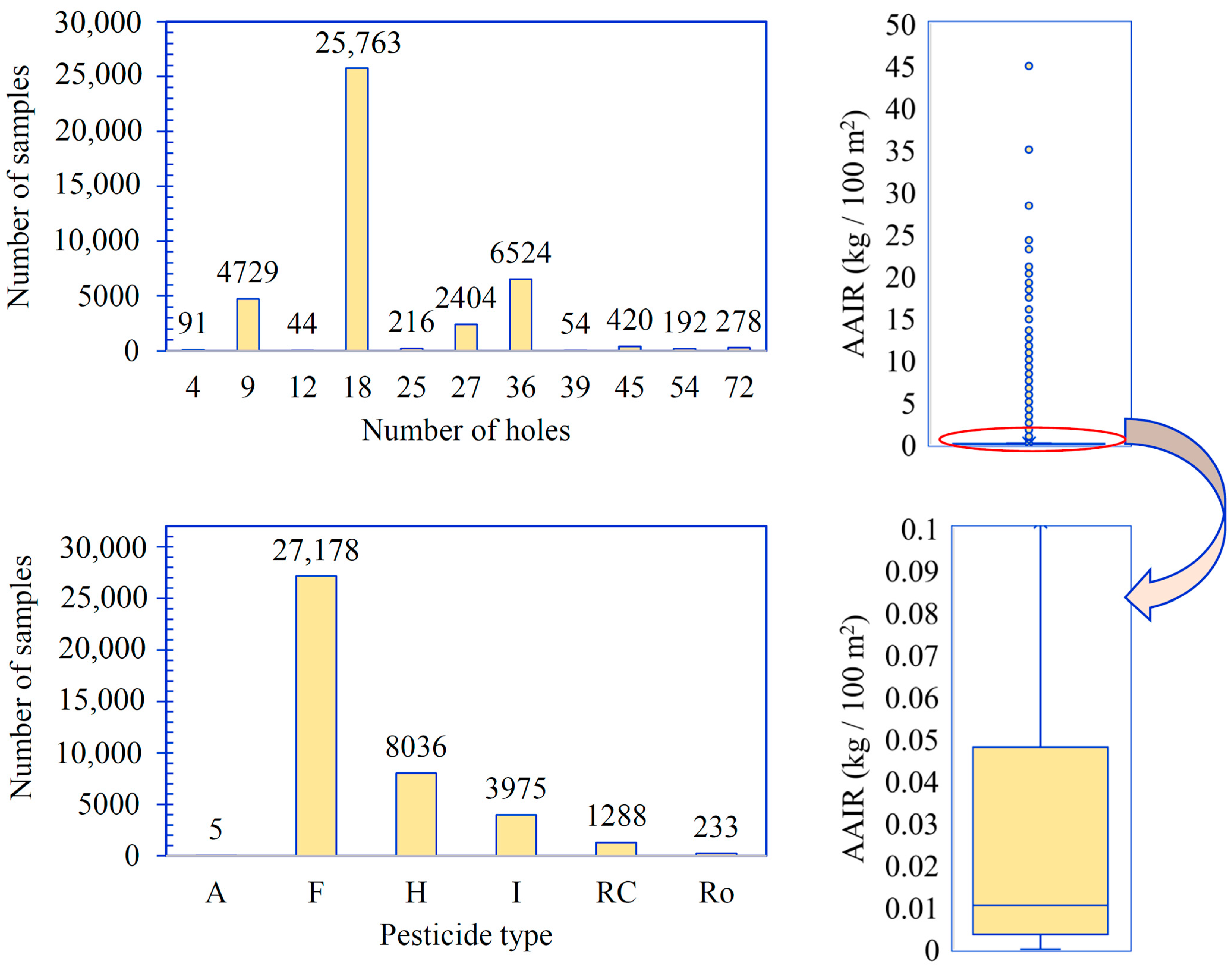
Figure 3 shows the distribution of the AAIR using a boxplot, as well as the number of different pesticide types (PT) and the number of holes (NH) for the cleaned dataset. For PT, more than 66% of all samples are fungicides (F), while this value equals 19.74%, 9.76%, and 3.16% for herbicides (H), insecticides (I), and growth regulators (RC), respectively. The percentage of other pesticide types is less than 1%. More than 63% of all samples are related to the NH = 18, while this value for golf courses with 9, 27, 36, and 45 holes is 11.56%, 5.9%, 16.02%, and 1.03%, respectively. The percentage of unique pesticide use applications on golf courses is less than 1%. Due to Figure 3, most of the AAIR samples are less than 0.1 kg/100 m2 (red line selected in the box plot).
Figure 3 shows that the maximum value of AAIR is approximately 45 kg 100 m−2. The first quartile, third quartile, and average of this variable are 0.00345, 0.048, and 0.1015 kg 100 m−2, respectively. The average of samples for AAIR is higher than the third quartile. It means most of the samples are significantly smaller than those larger than the third quartile. Considering this issue, which is clearly shown in Figure 3, there is a complex problem that requires a unique strategy. Therefore, in this study, a training method was proposed that showed not only good performance, on average, but also provided acceptable performance in all domains. The description of the developed model is presented in the following section.

2.2. Modeling Approach

2.2.1. Convolution Neural Network (CNN)

A convolutional neural network (CNN) is a neural network whose layers are interconnected locally [11], which overcomes the challenge of reduced speed in the learning of traditional artificial neural networks (ANN) [12]. The CNN technique is a deep learning-based algorithm consisting of multiple layers of neurons. The initial layer, known as the convolution layer (CL), processes input data by examining small squares and maintaining pixel connections. The CL requires two inputs: a kernel or filter and an image matrix. Following the convolutional layer, an activation layer can be utilized, typically in the form of a nonlinear function. The use of newly developed activation functions enables the creation of networks with simpler structures or faster convergence.
Typically, rectified linear unit (ReLU) functions, which are commonly used as activation functions, are zeros and ones, making them the most effective and typical activators [13]. ReLU activation functions provide numerous notable benefits. These include circumventing the vanishing gradient issue, computational efficiency [14], representation of sparsity that simplifies and accelerates model training, and linear behavior [15]. The threshold operation of the ReLU activation function is expressed as follows:
f ( x ) = 0 0 x x 0
The pooling layer (PL), also referred to as downsampling, plays a crucial role as the third layer in CNN. Its primary function is to retain the most important information while reducing the number of parameters, especially when dealing with large images. Various types of spatial pooling methods can be employed, such as Max, Average, and Sum. The purpose of the pooling layer is to decrease the spatial resolution of the feature maps while preserving essential details. This reduction in resolution leads to a significant reduction in computation cost by greatly reducing the number of parameters, which, in turn, helps mitigate the risk of overfitting and enhances the generalization capabilities of the network. Additionally, pooling offers the advantage of insensitivity to translations, minor transformations, and distortions in the input volume, thus contributing to the robustness of the CNN architecture [16].
In a deep neural network, the final layer performs discriminative learning. Object classes are identified by this fully connected system. On the basis of images, project goals, and data, scholars have proposed a wide variety of different structures, such as AlexNet, ResNet, VGGNet, LeNet, GoogleNet, and ZFNet [17]. Agricultural researchers have successfully used CNN-2D in the past, so this structure was used in the current study as well [18,19,20,21]. Moreover, in order to utilize the CNN architecture, the input data need to be represented as images, which requires four dimensions. However, in the case of the current study, the primary input data were one-dimensional. Therefore, a conversion process was necessary to transform the data into image format prior to commencing the modeling phase. This conversion allowed for the collected data for AAIR to be appropriately represented as images, enabling the utilization of the CNN for further analysis and modeling.
At the onset of the convolutional layer in the employed network, a hundred filters were utilized to capture and emphasize the correlations between nearby features within the data. This approach is particularly suitable for data that exhibit high correlations resembling image-like structures. A filter size of 10 × 1 was chosen to facilitate the learning of correlations between features throughout the training phase of the network. By incorporating this filter, the network could effectively extract and highlight correlation features by considering the interplay among all features. The ReLU activation function was employed in this layer to introduce non-linearity and enhance the expressive power of the network.
This was followed by the normalization layer. Batch normalization, a widely adopted technique in deep learning, was employed in this study. It served multiple purposes, including accelerating the learning process by mitigating overfitting and providing regularization. Unlike traditional normalization methods applied to raw data, batch normalization operates between the layers of the neural network. Instead of analyzing the entire dataset at once, it divides the data into mini-batches for analysis. Additionally, a dropout layer with a rate of 50% was introduced. This layer plays a crucial role in the learning process by randomly setting half of the outputs from the previous layer to zero during each iteration. This dropout mechanism facilitates the learning of diverse aspects of the data and avoids overfitting by preventing the inputs of the next layer from becoming overly dependent on specific features. This layer was followed by a max pooling layer, which decreased its dimensions. The max pooling filter size was 3 × 1. By using this layer, the weight of the network was considerably decreased, and its computational load was extremely reduced. The next layer was the fully connected layer, with the ReLU as its activation function. The final layer was a fully connected layer consisting of one neuron and one regression layer to generate the final result.

2.2.2. Random Forest (RF)

The RF [22] is an ensemble learning technique that consists of multiple decision classification trees. Each decision tree in the RF algorithm is built by randomly selecting a subset of features from the available set. The predictions from these individual trees are then combined using an average or majority voting approach, depending on the specific problem being addressed. This ensemble strategy allows RF to make more accurate and robust predictions compared with a single decision tree. The random feature selection and aggregation of results contribute to the overall effectiveness of the RF algorithm. Consider {G (x, βi), i = 1, …, L)} (where x is the characteristic variable, βi is the random variable, and L denotes the number of decision trees) as the input data set and G (x, βi) as the result of the single decision tree (SDT); then, the results of all SDTs are averaged to form the estimated result of the RF:
G ¯ ( x ) = 1 L i = 1 L G ( x , β i )
where G ¯ ( x ) is the RF-based estimated value of the target variable.
The RF modeling process employs a bagging approach with replacement, where samples are randomly drawn with replacement from the original set of samples. This is carried out k times, ensuring that the sample size of each decision tree in the RF is the same as the original training set. In the RF modeling process, out-of-bag (OOB) sampling is used to create a sample consisting of data that were not selected during each iteration. It is important to note that samples may be chosen multiple times or not chosen at all. A certain percentage of all samples, typically two-thirds, is selected for model calibration and is referred to as the in-bag (IB) samples. The RF model’s generalizability is assessed through internal cross-validation using the remaining out-of-bag (OOB) samples. These OOB samples are not used in the model training and serve as an independent evaluation set to estimate the model’s performance.
Each randomly selected training set in the RF model generates a regression tree (RT) with a specified number of input features, denoted as M. When constructing the RT, a subset of m feature variables is chosen as candidates for the branch nodes, where m is less than or equal to M. The selection of these feature variables is arbitrary. The branching superiority principle is then applied to determine the optimal splitting strategy at each node of the tree. This principle guides the selection of the feature variable and splitting point that results in the most significant improvement in the model’s performance [23]. By iteratively applying this process, a set of regression trees is generated in the RF model.
In each RT generated using the classification and regression tree (CART) method, branches are allowed to grow freely from the top to the bottom without pruning [24]. By applying this method, a set of k RTs is created to form a random forest. The prediction results of each RT are then averaged to obtain the final results of the forest. This ensemble approach combines the predictions from multiple trees to improve the overall accuracy and robustness of the model. To assess the generalizability of the model, the OOB data, which consist of the samples that were not selected during the training process, are used for evaluation.

2.2.3. Hybrid Methodology

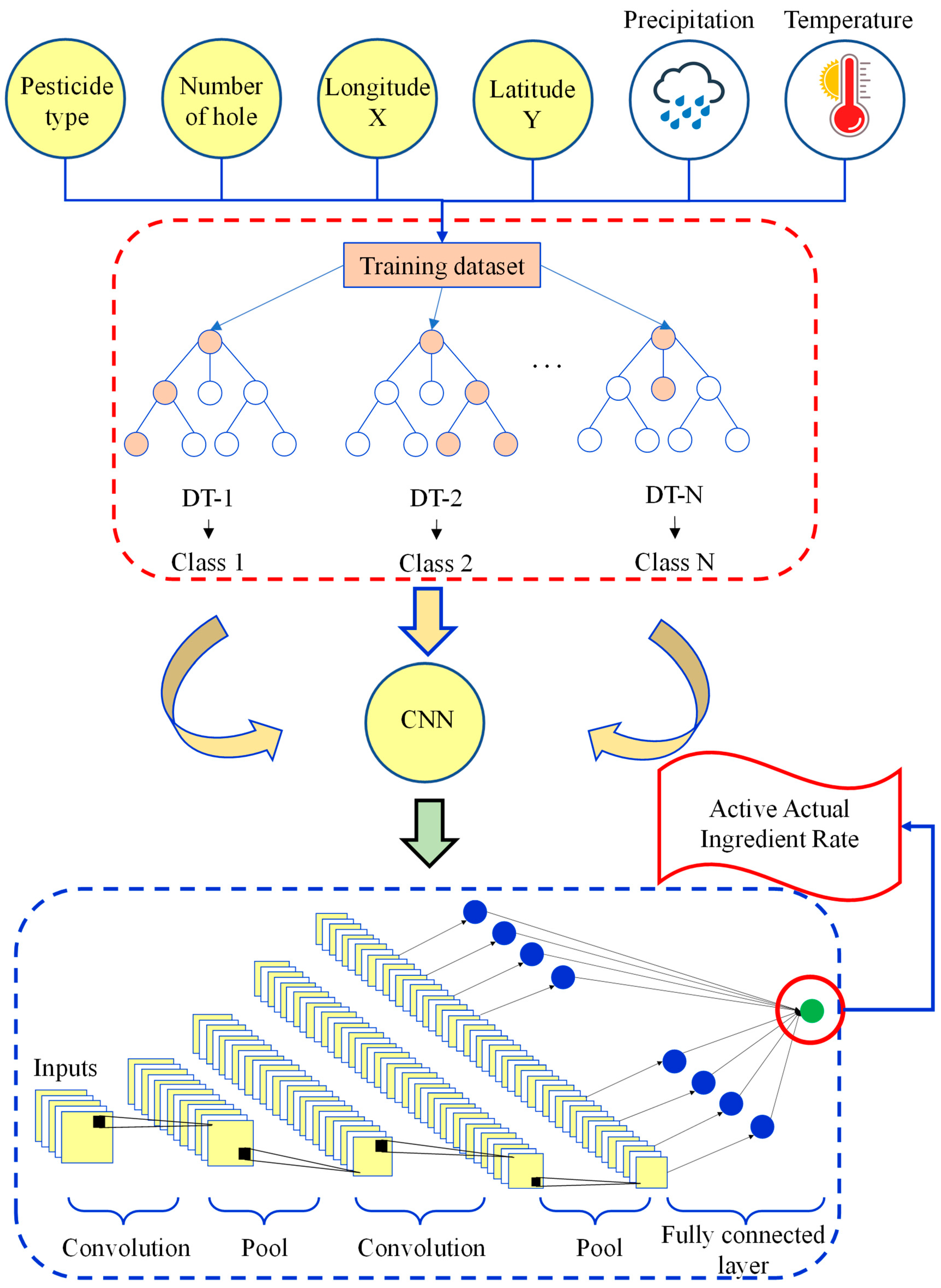
The conceptual framework depicting the structure of the hybrid model developed in this study is presented in Figure 4. The initial step involved loading the data and categorizing it into two main groups: the training and testing datasets. The widely recognized random selection without replacement (RSWR) approach [25,26] commonly used in machine learning modeling was employed to accomplish this. Through RSWR, 30% of the total samples were selected for the testing stage, while the remaining samples were utilized for training the model. The testing dataset, which did not contribute to the model training, was employed solely for evaluating the performance of the machine learning-based model.
The second step involved defining user-defined parameters for both individual methods, the RF and CNN (refer to Table 1). Moving on to the third step, the training dataset was utilized to generate distinct random vectors. These vectors served as input for producing decision trees. Subsequently, the decision trees generated were used in a voting process to determine the final results of the RF method. Indeed, the modeling process commenced with the utilization of the random forest (RF) algorithm. The RF algorithm generated class predictions as outcomes, which, in turn, facilitated the automatic division of the dataset into distinct classes. In Figure 4, the class denoted as DT-1 corresponds to the initial class produced by the RF algorithm. Subsequently, for each class generated by the RF, the CNN was employed to conduct further analysis of the data within that particular class. Indeed, the modeling process involved two distinct phases. Firstly, the random forest (RF) algorithm was employed to identify the optimal classes. Subsequently, separate models were developed for each organized class identified by the RF using the CNN. The number of models developed for each scenario were denoted as S1 to S4 according to Equations (6)–(9), which corresponded to the number of classes determined by the RF algorithm. The models described in Equations (6)–(9) share common input variables. These inputs include the number of holes (NH), pesticide types (PT), coordinates (X and Y), precipitation (P), and temperature (T). Furthermore, the output variable for all models is the actual active ingredient rate (AAIR), as defined in Equation (1). Finally, the performance evaluation of the model was extended beyond the training dataset and included the testing dataset. If the obtained results met the required criteria, the modeling process concluded. However, if the results were not satisfactory, the parameters of RF and CNN were readjusted. The process of identifying optimal classes using RF and modeling each class using CNN was repeated iteratively until acceptable results were attained. Ultimately, the RF and CNN were integrated into a unified framework known as the RFCNN.
As mentioned in Table 1, the applied optimizer in CNN was “Adamax”, which offers several advantages, including adaptive learning rates, effective handling of sparse gradients, robustness to different scale parameters, memory efficiency, and convergence of non-stationary objectives.
The functional relationship between the inputs and outputs in the current study was defined as follows:
A A I R = f ( Characteristic of Golf Courses , Coordinates , Meteorological Variables )
Considering the number of holes and pesticide types as characteristics of golf courses, as well as precipitation and temperature as meteorological variables, the above relationship was rewritten as follows:
A A I R = f ( N H , P T , X , Y , P , T )
where NH is the number of holes, PT is the pesticide types, X and Y are the longitude and latitude of the golf courses, respectively, P is the precipitation, T is the temperature, and AAIR is the actual active ingredients rate (kg 100 m−2).
Meteorological parameters provided in the functional relationship in Equation (4) are total precipitation and average temperature. However, the period during which these parameters are to be considered can have an influence on the algorithm output, so different scenarios were evaluated. The different scenarios are detailed in Equations (6)–(9):
S 1 : A A I R = f ( N H , P T , X , Y , P S e a s o n , T S e a s o n )
S 2 : A A I R = f ( N H , P T , X , Y , P S u m m e r , T S u m m e r )
S 3 : A A I R = f ( N H , P T , X , Y , P W i n t e r , T W i n t e r )
S 4 : A A I R = f ( N H , P T , X , Y , P W i n t e r , T W i n t e r , P S u m m e r , T S u m m e r )
where NH is the number of holes, PT is the pesticide type, PSeason and TSeason are total precipitation and average temperature, respectively, recorded during the golf playing season (May to November), PSummer and TSummer are total precipitation and average temperature, respectively, during the summer months (April to October), and PWinter and TWinter are total precipitation and average temperature, respectively, during the winter months (November to March).

2.3. Goodness of Fit

Appraising models based solely on one criterion does not suffice due to the stochastic nature of the target variable (i.e., AAIR in the current study). The developed models for AAIR forecasting were, therefore, checked using a group of quantitative measurements, including coefficient of determination (R2), Nash–Sutcliffe efficiency (NSE), root mean square error (RMSE), mean absolute error (MAE), normalized RMSE (NRMSE), and the percentage bias I (PBIAS). The mathematical definitions of the mentioned indices are defined as Equations (10)–(15):
R 2 = 1 SSR = i = 1 N A A I R i O A A I R i M SST = i = 1 N A A I R i O A A I R O ¯
N S E = 1 i = 1 k A A I R i E A A I R i O 2 i = 1 k A A I R i O A A I R O ¯ 2
R M S E = 1 k i = 1 k A A I R i E A A I R i O 2
M A E = 1 k i = 1 k A A I R i E A A I R i O
N R M S E = R M S E A A I R O ¯
P B I A S = i = 1 k A A I R i E A A I R i O i = 1 k A A I R i O × 100
where SSR is the sum of squares due to regression, SST is the total sum of squares, A A I R i O and A A I R i E denote the value of the ith observed and estimated (respectively) samples of the actual active ingredient rate (AAIR), A A I R O ¯ is the average of the observed AAIR samples, and k is the number of samples.
The R2 was applied to measure the difference between the variance and mean of the observed and estimated samples. Using it alone for model evaluation is not recommended due to its sensitivity to outliers [27,28]. The difference between the observed and estimated and its squared were represented by MAE and RMSE, respectively. These indices could be compared simply since the error was computed in the same units as the estimated target variable. By using the average magnitude and size of the error, MAE calculated the errors without considering their direction. The most significant errors were given more weight by RMSE. Similar to MAE, the error directions were not considered. In addition, the NRMSE was applied to use RMSE as a dimensionless index [29], sometimes called the scatter index. As a result, the RMSE, NRMSE, as well as MAE should be used in conjunction with other indices.
The range of NSE is [−1, 1], with NSE = 1 being the perfect value for this index. The condition NSE = 1 is achieved when the estimation error variance is zero. The PBIAS was applied to check the mean tendency of the developed model, lower or higher than the observed value. These metrics reflected the descriptive performances of the R2 [30], NSE [31], NRMSE [32], and PBIAS [33] provided in Table 2. It should be noted that there is no descriptive performance for MAE and RMSE because they are dimensional indices, and the lower the values of these indices, the higher the performance of the model.

3. Results and Discussions

3.1. RFCNN-Based Estimation of AAIR in Different Scenarios

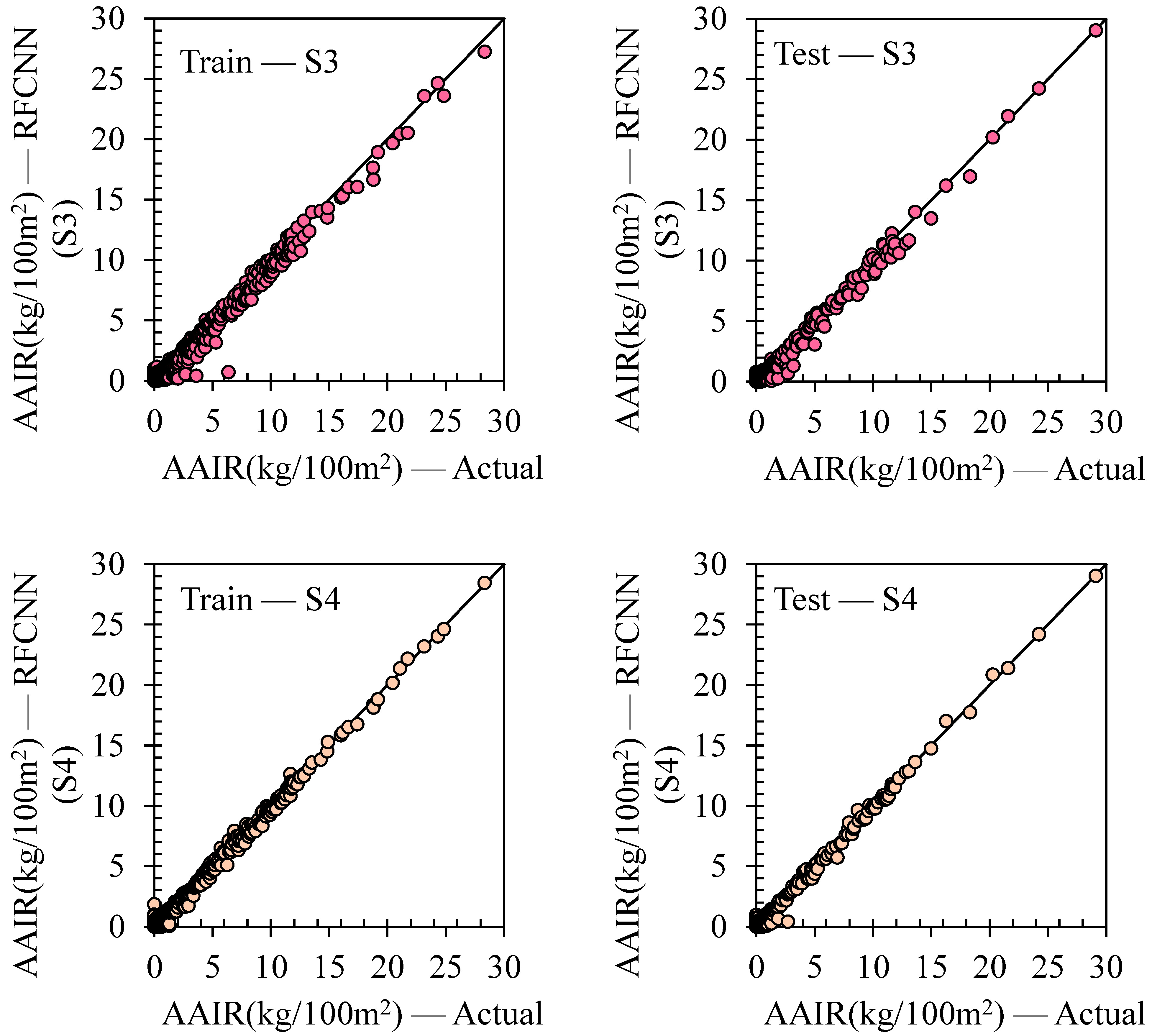
Figure 5 shows the scatter plots of the RFCNN in AAIR forecasting at both training and testing stages through four different scenarios (i.e., S1 to S4, defined as Equations (6)–(9), respectively). Table 3 provides the statistical indices of the RFCNN in AAIR forecasting at both the training and testing stages for the four different scenarios. The main difference between these scenarios was related to the period considered for the total precipitations and mean temperature. The other input variables, including the number of holes (NH), pesticide type (PT), and geographical coordinates (X, Y), were constant in all scenarios.
The provided scatter plot for S1 in Figure 5 indicates that the RFCNN model performed well for this scenario at both the training and testing stages. This is confirmed by the quantitative evaluation of the RFCNN presented in Table 3. According to the index of model performance presented in Table 2, R2, NSE, NRMSE, and PBIAS of the model using S1 are qualified as “very good”. In addition, the RMSE and MAE of this model are extremely close to zero, indicative of good model performance. It should be noted that the difference between the statistical indices for the two stages (training and testing) is insignificant in this scenario. Indeed, these results suggest that the developed model for AAIR forecasting using S1 has good generalizability, and its use of data that did not play a role in model training, such as data that will be recorded in the future, will perform well.
For S2, the scatter plot (Figure 5) and the statistical indices (Table 3) obtained for both the training and testing stages show the acceptable performance of the RFCNN model in the AAIR estimation using the input variables defined in Equation (7). According to Table 2, the descriptive performance of the RFCNN in AAIR estimations using S2 based on the R2, NSE, NRMSE, and PBIAS is qualified as “very good”. However, R2 and NSE of S2 were, respectively, 1.51% and 1.88% lower than those for S1, and the RMSE, MAE, and NRMSE of the model using S2 were, respectively, 150.15%, 107.84%, and 150.51% higher than those for S1. In addition, the PBIAS of S2 was three times higher than those obtained for S1. Furthermore, using total precipitation and average temperatures from April to October (PSummer, TSummer) (S2) instead of May to November (PSeason, TSeason) (S1) resulted in a significant reduction in the performance of the model for the AAIR estimated at the test stage, which negatively affected the model generalizability. This reduction of performance indicates that some of the samples were estimated to be lower than the actual AAIR with high error, especially in the range of 0 < AAIR (kg 100 m−2) < 6. Therefore, it can be concluded that the use of meteorological variables recorded only for summer cannot predict AAIR values with reasonable accuracy in all ranges of the AAIR.
The RFCNN model using S3 generally performed well in AAIR forecasting (Figure 5), with R2, NSE, PBIAS, and NRMSE at both the training and testing stages (Table 3) qualified as “very good” according to the classification presented in Table 2. However, a comparison of the mentioned indices for S3 with those obtained with S1 indicates that the R2 and NSE of S3 were, respectively, 1.23% and 1.55% lower than those for S1, and the RMSE, MAE, and NRMSE of the S3 were, respectively, 132.815%, 112.83%, and 132.82% higher than those for S1. In addition, the PBIAS of S3 (training and testing) are five times higher than those for S1. A comparison of S2 with S3 indicates that the R2, NSE, and MAE of S3 were, respectively, 0.28%, 0.34, and 2.35% higher than those for S2, and the RMSE and NRMSE of the S3 were both 7.45% lower than those for S2. However, in both the training and testing stages of S3, different samples were underestimated with high relative error, especially in the range of 0 < AAIR (kg 100 m−2) < 6, similar to what was observed with S2. Thus, the use of total precipitation and average temperature from April to October (PSummer and TSummer) or November to March (PWinter and TWinter) (i.e., S2 and S3) led to a decrease in the performance of the model compared with the scenario that considered the value of these two variables from May to November (i.e., S1). Moreover, the results of all statistical indices except MAE showed that using total precipitation and average temperature from November to March (winter) resulted in a more accurate model than using the values of these parameters from April to October (summer).
The provided scatter plots in Figure 5 demonstrate that the estimated AAIR by S1 and S4 were very similar, performing well in all ranges of AAIR. The number of input variables in S4 was higher than in the other scenarios because total precipitation and the average temperature in S4 combined the summer (April to October) and the winter (November to March) periods. The descriptive performance of R2, NSE, PBIAS, and NRMSE for S4 at both training and testing stages (Table 3) are qualified as “very good” according to Table 2. The statistical indices of S4 and S1 provided in Table 3 indicate that S1 had higher R2 and NSE than S4 by 0.6% and 0.64%, respectively, and its RMSE, MAE, and NRMSE were lower by 71.03%, 58.91%, and 71.03%, respectively, than S4. Additionally, the PBIAS values of S4 (training and testing) were approximately two times greater than those of S1. On the basis of the explanations provided, the scatter plots presented in Figure 5, as well as the statistical indices in Table 3, the model developed in scenario 1 (Equation (6)) was selected as the best model.

3.2. Sensitivity Analysis

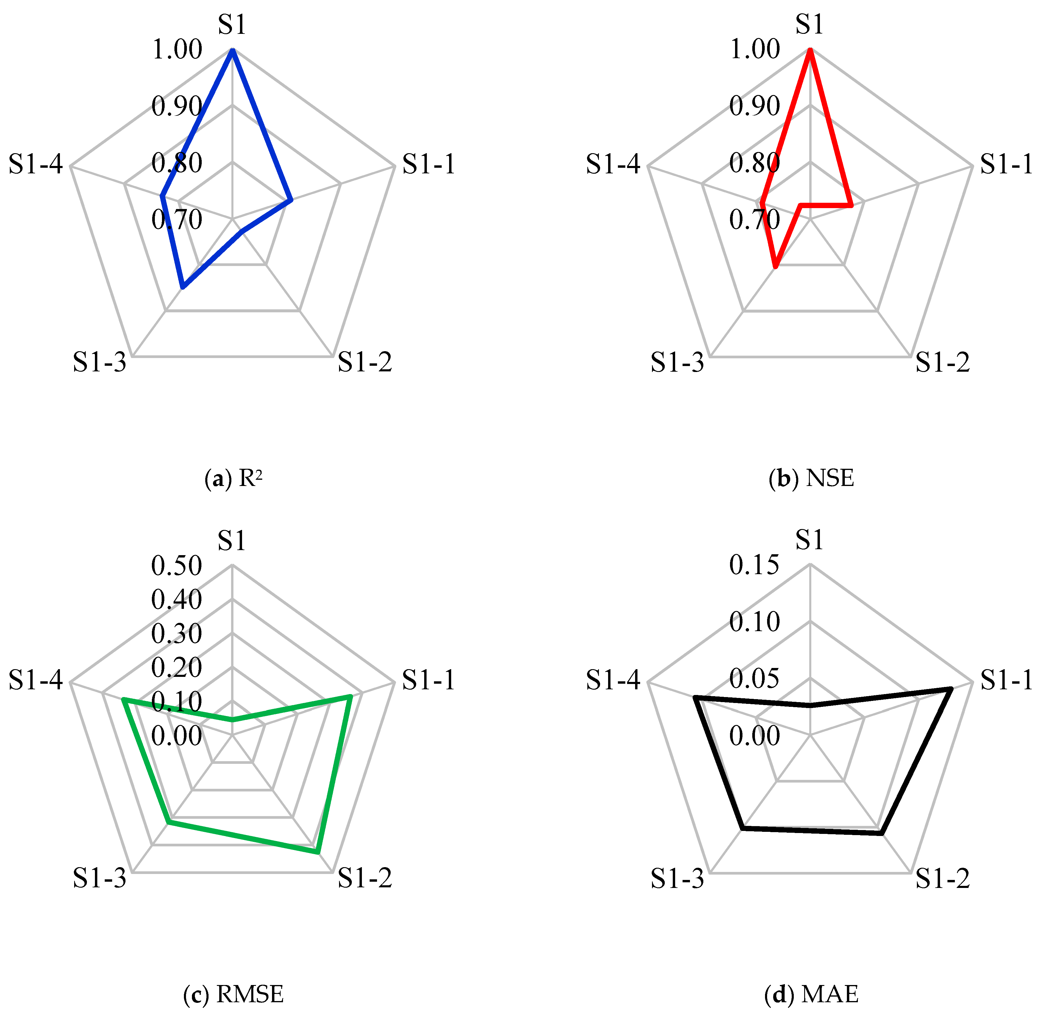
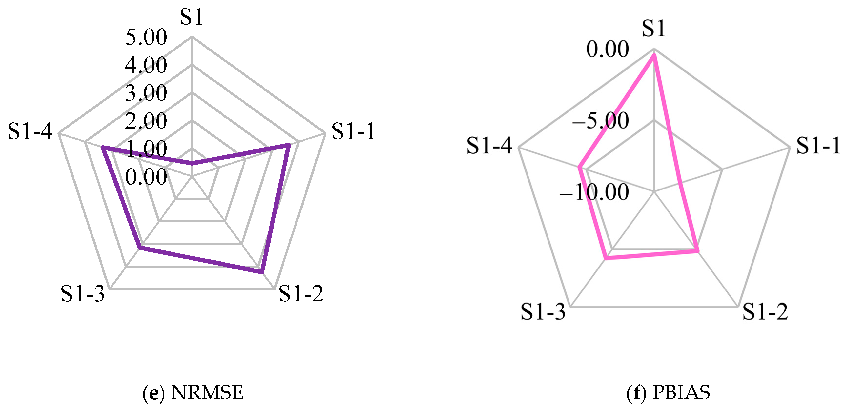
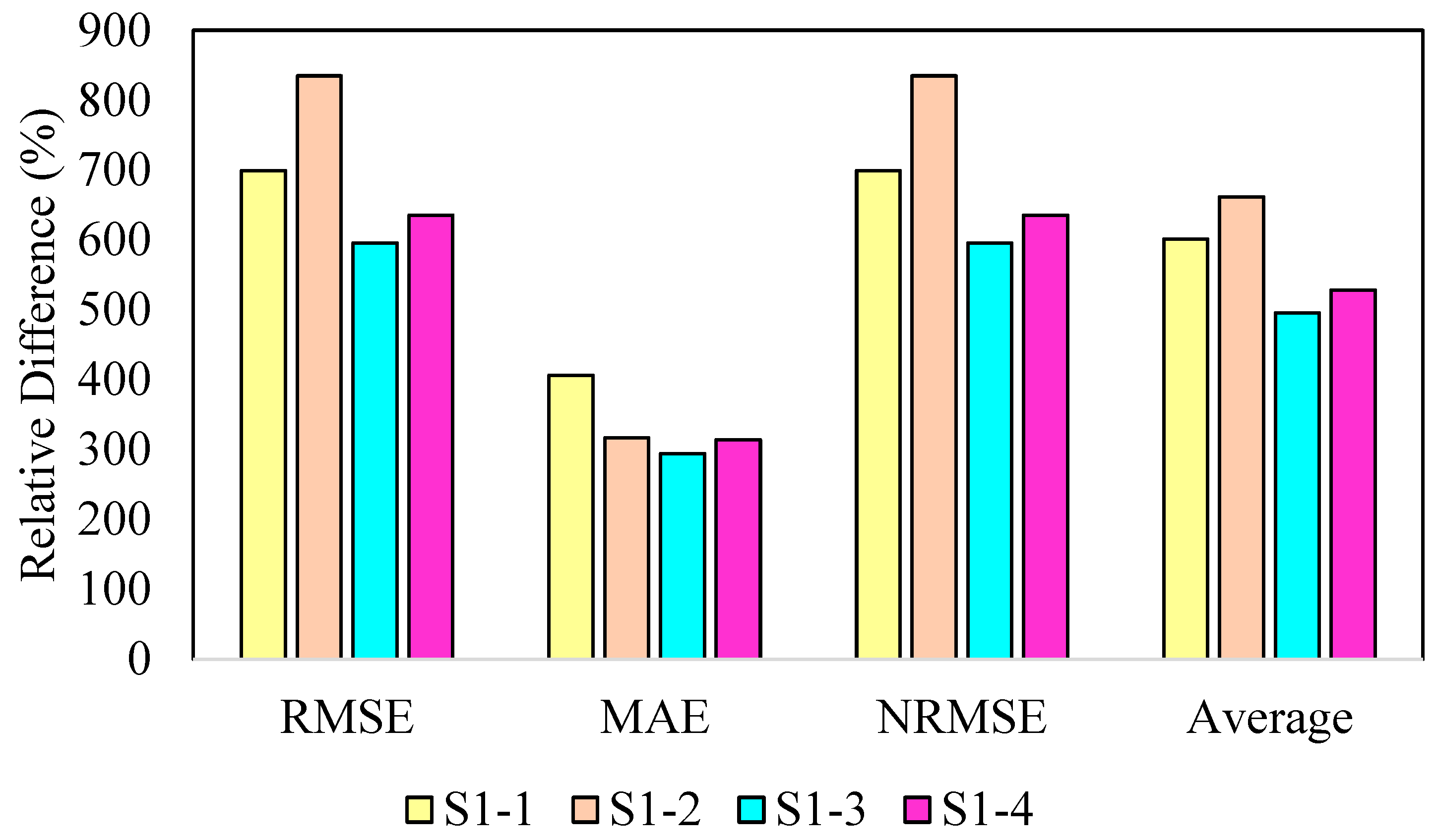
To check the effect of each input variable on the AAIR forecasting on the basis of the best scenario (i.e., S1), four different sub-scenarios were defined and are presented in Table 4. Each sub-scenario has five inputs, so the difference between S1-1 and S1-4 is the lack of using either the number of holes, the pesticide type, the total precipitation, or the average temperature as an input variable. The effect of each independent input variable on the AAIR forecasting using the developed RFCNN is presented in Figure 6. Removing the average temperature from May to November as the model input (i.e., S1-1) had a negative effect on the modeling results, so that the correlation-based indices of the S1-1 (R2 = 0.81; NSE = 0.78) decreased by more than 19% compared with S1. Despite the decrease in the values of these two indices, their descriptive performance still is “very good” according to Table 2. The relative differences in statistical indices of S1 with S1-1, S1-2, S1-3, and S1-4 are presented in Figure 7. The RMSE, MAE, NRMSE, and PBIAS of the S1-1 (RMSE = 0.36; MAE = 0.13; NRMSE = 3.63; and PBIAS = −8.09) were more than 6, 4, 6, and 16 times the values of these indices for S1 (RMSE = 0.05; MAE = 0.03; NRMSE = 0.45; and PBIAS = −0.47), respectively. According to Table 2, the descriptive performances of this model based on the NRMSE and PBIAS are “very good” and “good”, respectively.
Removing PSeason as an input in the model (S1-2) decreased the RFCNN performance in the AAIR forecasting (R2 = 0.73; NSE = 0.64; RMSE = 0.43; MAE = 0.11; NRMSE = 4.24; and PBIAS = −4.84). As shown in Figure 6, the S1-2 not only provided weaker performance compared with the S1 but also the performance of this model in terms of R2, NSE, RMSE, and NRMSE was weaker than S1-1.
After evaluating the effect of the meteorological variables (i.e., total precipitations and average temperature), the effect of golf course characteristics was assessed. Removing the pesticide type as an input variable (S1-3) significantly decreased the modeling accuracy so that the R2 and NSE of the S1-3 were decreased by more than 14% and 19%, respectively, compared with S1 (Figure 6). These relative differences between S1-3 and S1 for other indices were in the range of 294% to 799% (Figure 7). The effect of the number of holes was higher than the pesticide type, so that the R2 and NSE of the S1-4 were decreased by more than 16% and 20%, respectively, compared with S1 (Figure 6). The relative differences between S1-4 and S1 for the other indices were in the range of 313% to 856% (Figure 7).
On the basis of the provided explanations and results in Figure 5, Figure 6 and Figure 7, it can be seen that removing any golf course characteristics and meteorological variables resulted in a remarkable reduction in modeling accuracy. The total precipitation from May to November (PSeason) and the number of holes (NH) were the most effective variables related to the meteorological variables and gold course characteristics, respectively. Generally, the total precipitation during the golf season (PSeason) had the highest impact on the AAIR forecasting using the developed RFCNN method.
As shown in Table 4, both longitude (X) and latitude (Y) were considered in all sub-scenarios. The model discussed in this context had the capability to be applied in various locations by incorporating latitude and longitude information. However, if latitude and longitude were excluded from the model, its performance would be greatly diminished. Indeed, the omission of latitude and longitude resulted in a significant decrease in model performance. The R2 values for the models with all provided inputs in Equation (6), except latitude or longitude, were 0.57 and 0.45, respectively. Hence, it is evident that taking into account the specific characteristics of the study area held substantial importance when modeling pesticide usage on the golf courses.

3.3. Advantages, Limitations, and Future Improvements

In the current investigation, the introduced hybrid RFCNN as an integration of the random forest (RF) and convolution neural network (CNN) was exceptionally successful in forecasting the pesticide actual active ingredient rate (AAIR) (kg 100 m2) used on golf courses in Québec. The main advantages of the current research study were threefold: (1) precise estimation of the AAIR, (2) automatic classification of the data to overcome existing problems in the range of the AAIR values (the third quartile of the AAIR was lower than the average of all samples, see Figure 3), and (3) testing of different scenarios combining golf course characteristics and meteorological variables, as was recommended in a recently published paper [9]. The developed model based on the selected scenario (i.e., S1) can be used as a practical tool for forecasting AAIR for future years on the basis of the different climate change scenarios. Indeed, the values of the meteorological variables (i.e., total precipitations and average temperatures) can be obtained on the basis of the different climate change scenarios to calculate and report the AAIR value and its trend in future years.
In the current study, a CNN was used to map the input variables to the AAIR nonlinearly for each class that the RF automatically created. The main advantages of the RF were its exceptional accuracy in classification, its ability to determine the significance of variables, and its non-parametric nature [34]. In comparison with the traditional artificial neural network, a CNN is capable of automatically detecting crucial features without the need for human involvement. Indeed, this makes the training of the model more accurate and requires fewer parameters to be learned through the training phase.
One limitation of the present study is that a trial-and-error process was used to determine the user-defined parameters of the CNN. To find the optimal values of this technique, a newly developed optimization algorithm, such as the cooperation search algorithm [35], fire hawk optimizer [36], or white shark optimizer [37], could be integrated with the CNN. The results of the current study could then be compared with the CNN optimized using optimization algorithms to determine whether it would affect model performance.
The challenges in the AAIR analysis and developing an effective ML-based model are categorized into two main groups: data and modeling challenges. The main challenges with data were not only a large number of samples (i.e., 40,715) but also the wide range of the AAIRs so that the average of all samples was higher than the 3rd quartile of the samples. Therefore, it was time-consuming to model many samples, especially for the current study for which modeling needed a high number of iterations to achieve the most optimum results in all automated created groups of samples by the RF. The main modeling challenges for a computer with an Intel Core i7 processor and 16 GB RAM were (1) the high number of iterations required for the developed hybrid model, (2) low memory in using the newly developed hybrid machine learning model for the forecasting of the golf course characteristics [9], and (3) finding the optimum values of the developed RFCNN.

4. Conclusions

The current study developed a new hybrid machine learning model known as RFCNN to accurately forecast pesticide application rates on golf courses, expressed as the actual active ingredient rate (AAIR), in the Québec province of Canada. The RFCNN is an integration of the random forest (RF) and the convolution neural network (CNN). The RF was used to classify all samples in order to overcome the existing problems in working with a wide range of AAIR values, while the CNN was applied to map the independent input variables to the dependent target variable (i.e., AAIR). Sensitivity analysis of the developed model revealed that the meteorological parameters played an important role in the pesticide AAIR forecasting. Total precipitations and average temperatures recorded during the golf season (May to November) ranked first and second in importance in the RFCNN model, while pesticide types and the number of holes of the golf course ranked third and fourth, respectively.
By using this model, golf course managers in Québec may be able to forecast pesticide use more accurately and set pesticide-reduction targets in accordance with existing legislation. In addition, this model can be used by regulatory authorities and agronomists to refine and improve pesticide reduction processes on golf courses. For example, beneficial economic measures could be implemented for golf courses that use fewer pesticides than expected by the model, thus encouraging them to reduce their reliance on pesticides.
This model is a conditional method to predict the impact of climate change. While this current model was limited to pesticides used on golf courses in Québec, it could be adapted to other crops in different regions if data on pesticide applications and farm characteristics are available. Considering the spatial importance and pesticide use on some crops, using such a model could help us to understand better the factors affecting pesticide use and, thus, direct public policies to reduce the use of these products. Finally, this tool could also be used to predict the impact of climate change on pesticide use by applying contrasting temperature and precipitation scenarios on the basis of different greenhouse gas emissions models.

Author Contributions

Conceptualization, G.G. and J.F.; methodology, G.G. and I.E.; software, I.E.; formal analysis, G.G. and I.E.; investigation, G.G., I.E. and H.B.; writing—original draft preparation, G.G. and I.E.; writing—review and editing, G.G., J.F. and H.B.; visualization, G.G. and I.E.; project administration, G.G., J.F. and H.B.; funding acquisition, G.G. All authors have read and agreed to the published version of the manuscript.

Funding

This project was funded by the Canadian Turfgrass Research Foundation and the Québec Turfgrass Research Foundation.

Institutional Review Board Statement

Not applicable.

Data Availability Statement

Restrictions apply to the availability of these data.

Acknowledgments

The authors thank the Ministère de l’Environnement et de la Lutte aux Changements Climatiques du Québec for giving us access to the database.

Conflicts of Interest

The authors declare no conflict of interest.

References

  1. Metcalfe, T.L.; Dillon, P.J.; Metcalfe, C.D. Detecting the Transport of Toxic Pesticides From Golf Courses into Watersheds in the Precambrian Shield Region of Ontario, Canada. Environ. Toxicol. Chem. 2008, 27, 811–818. [Google Scholar] [CrossRef] [PubMed]
  2. Kobayashi, Y.; Uchida, T.; Yoshida, K. Prediction of soil adsorption coefficient in pesticides using physicochemical properties and molecular descriptors by machine learning models. Environ. Toxicol. Chem. 2020, 39, 1451–1459. [Google Scholar] [CrossRef]
  3. Vaz, W.F.; D’oliveira, G.D.; Perez, C.N.; Neves, B.J.; Napolitano, H.B. Machine learning prediction of the potential pesticide applicability of three dihydroquinoline derivatives: Syntheses, crystal structures and physical properties. J. Mol. Struct. 2020, 1206, 127732. [Google Scholar] [CrossRef]
  4. Gilbert, E.P.K.; Edwin, L. A Review on Prediction Models for Pesticide Use, Transmission, and Its Impacts. Rev. Environ. Contam. Toxicol. 2021, 257, 37–68. [Google Scholar] [CrossRef] [PubMed]
  5. Jiang, B.; He, J.; Yang, S.; Fu, H.; Li, T.; Song, H.; He, D. Fusion of machine vision technology and AlexNet-CNNs deep learning network for the detection of postharvest apple pesticide residues. Artif. Intell. Agric. 2018, 1, 1–8. [Google Scholar] [CrossRef]
  6. Zhan-Qi, R.; Zhen-Hong, R.; Hai-Yan, J. Identification of different concentrations pesticide residues of dimethoate on spinach leaves by hyperspectral image technology. IFAC-PapersOnLine 2018, 51, 758–763. [Google Scholar] [CrossRef]
  7. He, L.; Xiao, K.; Zhou, C.; Li, G.; Yang, H.; Li, Z.; Cheng, J. Insights into pesticide toxicity against aquatic organism: QSTR models on Daphnia Magna. Ecotoxicol. Environ. Saf. 2019, 173, 285–292. [Google Scholar] [CrossRef]
  8. Miller, T.H.; Gallidabino, M.; MacRae, J.I.; Owen, S.F.; Bury, N.R.; Barron, L.P. Prediction of bioconcentration factors in fish and invertebrates using machine learning. Sci. Total. Environ. 2018, 648, 80–89. [Google Scholar] [CrossRef]
  9. Grégoire, G.; Fortin, J.; Ebtehaj, I.; Bonakdari, H. Novel Hybrid Statistical Learning Framework Coupled with Random Forest and Grasshopper Optimization Algorithm to Forecast Pesticide Use on Golf Courses. Agriculture 2022, 12, 933. [Google Scholar] [CrossRef]
  10. Gorelick, N.; Hancher, M.; Dixon, M.; Ilyushchenko, S.; Thau, D.; Moore, R. Google Earth Engine: Planetary-scale geospatial analysis for everyone. Remote Sens. Environ. 2017, 202, 18–27. [Google Scholar] [CrossRef]
  11. Lecun, Y.; Bottou, L.; Bengio, Y.; Haffner, P. Gradient-based learning applied to document recognition. Proc. IEEE 1998, 86, 2278–2324. [Google Scholar] [CrossRef]
  12. Lu, H.; Fu, X.; Liu, C.; Li, L.-G.; He, Y.-X.; Li, N.-W. Cultivated land information extraction in UAV imagery based on deep convolutional neural network and transfer learning. J. Mt. Sci. 2017, 14, 731–741. [Google Scholar] [CrossRef]
  13. Hasan, Z.; Hasan, K.Z.; Sattar, A. Burst Header Packet Flood Detection in Optical Burst Switching Network Using Deep Learning Model. Procedia Comput. Sci. 2018, 143, 970–977. [Google Scholar] [CrossRef]
  14. Glorot, X.; Bordes, A.; Bengio, Y. Deep sparse rectifier neural networks. In Proceedings of the Fourteenth International Con-ference on Artificial Intelligence and Statistics, Fort Lauderdale, FL, USA, 11–13 April 2011; pp. 315–323. [Google Scholar]
  15. Mercioni, M.A.; Holban, S. The most used activation functions: Classic versus current. In Proceedings of the 2020 International Conference on Development and Application Systems (DAS), Suceava, Romania, 21–23 May 2020; IEEE: Piscataway, NJ, USA, 2020; pp. 141–145. [Google Scholar]
  16. Botalb, A.; Moinuddin, M.; Al-Saggaf, U.M.; Ali, S.S.A. Contrasting Convolutional Neural Network (CNN) with Multi-Layer Perceptron (MLP) for Big Data Analysis. In Proceedings of the 2018 International Conference on Intelligent and Advanced System (ICIAS), Kuala Lumpur, Malaysia, 13–14 August 2018; pp. 1–5. [Google Scholar]
  17. Fang, W.; Ding, Y.; Zhang, F.; Sheng, V.S. DOG: A new background removal for object recognition from images. Neurocomputing 2019, 361, 85–91. [Google Scholar] [CrossRef]
  18. Kussul, N.; Lavreniuk, M.; Skakun, S.; Shelestov, A. Deep Learning Classification of Land Cover and Crop Types Using Remote Sensing Data. IEEE Geosci. Remote Sens. Lett. 2017, 14, 778–782. [Google Scholar] [CrossRef]
  19. Meng, S.; Wang, X.; Hu, X.; Luo, C.; Zhong, Y. Deep learning-based crop mapping in the cloudy season using one-shot hy-perspectral satellite imagery. Comput. Electron. Agric. 2021, 186, 106188. [Google Scholar] [CrossRef]
  20. Saleem, M.H.; Potgieter, J.; Arif, K.M. Automation in Agriculture by Machine and Deep Learning Techniques: A Review of Recent Developments. Precis. Agric. 2021, 22, 2053–2091. [Google Scholar] [CrossRef]
  21. Wang, C.; Liu, B.; Liu, L.; Zhu, Y.; Hou, J.; Liu, P.; Li, X. A review of deep learning used in the hyperspectral image analysis for agriculture. Artif. Intell. Rev. 2021, 54, 5205–5253. [Google Scholar] [CrossRef]
  22. Breiman, L. Random forests. Mach. Learn. 2001, 45, 5–32. [Google Scholar] [CrossRef]
  23. Pengcheng, L.; Xianguo, W.; Hongyu, C.; Tiemei, Z. Prediction of compressive strength of High-Performance Concrete by Random Forest algorithm. IOP Conf. Series Earth Environ. Sci. 2020, 552, 012020. [Google Scholar] [CrossRef]
  24. Lewis, R.J. An introduction to classification and regression tree (CART) analysis. In Proceedings of the Annual Meeting of the Society for Academic Emergency Medicine, San Francisco, CA, USA, 4–7 June 2000; Volume 14. [Google Scholar]
  25. Gharabaghi, B.; Bonakdari, H.; Ebtehaj, I. Hybrid evolutionary algorithm based on PSOGA for ANFIS designing in prediction of no-deposition bed load sediment transport in sewer pipe. In Proceedings of the Science and Information Conference, London, UK, 10–12 July 2018; pp. 106–118. [Google Scholar]
  26. Bonakdari, H.; Ebtehaj, I.; Gharabaghi, B.; Sharifi, A.; Mosavi, A. Prediction of Discharge Capacity of Labyrinth Weir with Gene Expression Programming. In Proceedings of the SAI Intelligent Systems Conference, London, UK, 3–4 September 2020; pp. 202–217. [Google Scholar] [CrossRef]
  27. Walton, R.; Binns, A.; Bonakdari, H.; Ebtehaj, I.; Gharabaghi, B. Estimating 2-year flood flows using the generalized structure of the Group Method of Data Handling. J. Hydrol. 2019, 575, 671–689. [Google Scholar] [CrossRef]
  28. Bonakdari, H.; Ebtehaj, I.; Samui, P.; Gharabaghi, B. Lake Water-Level fluctuations forecasting using Minimax Probability Machine Regression, Relevance Vector Machine, Gaussian Process Regression, and Extreme Learning Machine. Water Resour. Manag. 2019, 33, 3965–3984. [Google Scholar] [CrossRef]
  29. Gholami, A.; Bonakdari, H.; Ebtehaj, I.; Talesh, S.H.A.; Khodashenas, S.R.; Jamali, A. Analyzing bank profile shape of alluvial stable channels using robust optimization and evolutionary ANFIS methods. Appl. Water Sci. 2019, 9, 40. [Google Scholar] [CrossRef]
  30. Ayele, G.T.; Teshale, E.Z.; Yu, B.; Rutherfurd, I.D.; Jeong, J. Streamflow and sediment yield prediction for watershed priori-tization in the Upper Blue Nile River Basin, Ethiopia. Water 2017, 9, 782. [Google Scholar] [CrossRef]
  31. Moriasi, D.N.; Arnold, J.G.; Van Liew, M.W.; Bingner, R.L.; Harmel, R.D.; Veith, T.L. Model evaluation guidelines for systematic quantification of accuracy in watershed simulations. Trans. ASABE 2007, 50, 885–900. [Google Scholar] [CrossRef]
  32. Mihoub, R.; Chabour, N.; Guermoui, M. Modeling soil temperature based on Gaussian process regression in a semi-arid-climate, case study Ghardaia, Algeria. Géoméch. Geophys. Geo-Energy Geo-Resour. 2016, 2, 397–403. [Google Scholar] [CrossRef]
  33. Legates, D.R.; McCabe, G.J., Jr. Evaluating the use of “goodness-of-fit” measures in hydrologic and hydroclimatic model validation. Water Resour. Res. 1999, 35, 233–241. [Google Scholar] [CrossRef]
  34. Rodriguez-Galiano, V.F.; Ghimire, B.; Rogan, J.; Chica-Olmo, M.; Rigol-Sanchez, J.P. An assessment of the effectiveness of a random forest classifier for land-cover classification. ISPRS J. Photogramm. Remote Sens. 2012, 67, 93–104. [Google Scholar] [CrossRef]
  35. Feng, Z.-K.; Niu, W.-J.; Liu, S. Cooperation search algorithm: A novel metaheuristic evolutionary intelligence algorithm for numerical optimization and engineering optimization problems. Appl. Soft Comput. 2020, 98, 106734. [Google Scholar] [CrossRef]
  36. Azizi, M.; Talatahari, S.; Gandomi, A.H. Fire Hawk Optimizer: A novel metaheuristic algorithm. Artif. Intell. Rev. 2022, 56, 287–363. [Google Scholar] [CrossRef]
  37. Braik, M.; Hammouri, A.; Atwan, J.; Al-Betar, M.A.; Awadallah, M.A. White Shark Optimizer: A novel bio-inspired meta-heuristic algorithm for global optimization problems. Knowl.-Based Syst. 2022, 243, 108457. [Google Scholar] [CrossRef]
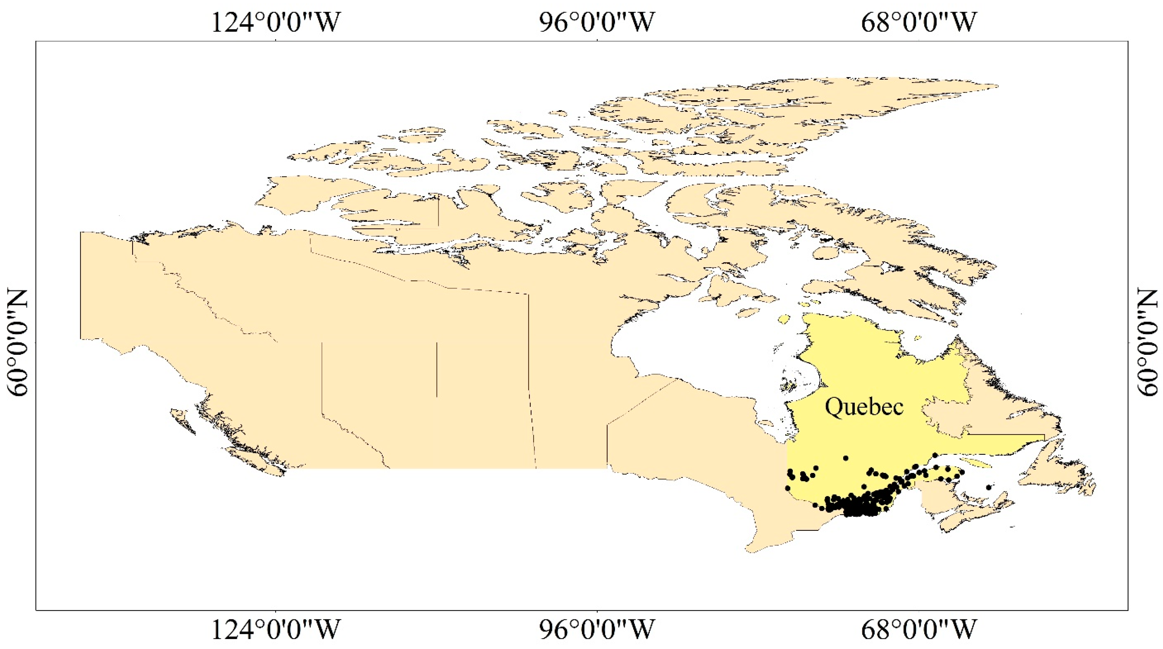
Figure 1. The location of the golf courses.
Agriculture 13 01163 g001
Figure 2. The distribution of the meteorological variables in southern Québec for three specific periods.
Agriculture 13 01163 g002aAgriculture 13 01163 g002bAgriculture 13 01163 g002c
Figure 3. Boxplot of the AAIR along with the number of different pesticide types and the number of holes. F—fungicides, H—herbicides, I—insecticides, RC—growth regulators, Ro—rodenticides, and A—others.
Agriculture 13 01163 g003
Figure 4. The conceptual scheme of the methodology adopted in the current study.
Agriculture 13 01163 g004
Figure 5. Scatter plots of the RFCNN in AAIR forecasting at both training and testing stages through four different scenarios.
Agriculture 13 01163 g005aAgriculture 13 01163 g005b
Figure 6. Effect of each independent input variable on statistical indices of model performance for AAIR forecasting using the developed RFCNN.
Agriculture 13 01163 g006aAgriculture 13 01163 g006b
Figure 7. The relative difference of statistical indices of model performance of S1 with S1-1, S1-2, S1-3, and S1-4.
Agriculture 13 01163 g007
Table 1. The settings of the user-defined parameters for developed CNN.
MethodParameterSetting
CNNOptimizer Adamax
Dropout rate 0.5
Learning rate 0.001
Weight decay 0.0005
Number of epochs 5000
Activation function ReLU
Initial learning rate 0.1
Max pooling kernel size 3 × 1
Convolutional kernel size10 × 1
Number of convolution units10
RFBag size percentage100
Batch size100
Maximum depth of the tree5
Number of decimal places2
Number of execution slots1
Number of features1
Number of iterations100
Seeds10
Table 2. Descriptive performance of various indices.
IndexR2NSEPBIASNRMSE
DescriptiveperformanceUnsatisfactoryR2 < 0.5NSE < 0.4PBIAS > ±25% 30% < NRMSE
Acceptable-0.4 < NSE < 0.5--
Satisfactory0.5 < R2 < 0.60.5 < NSE < 0.65±15% > PBIAS > ±25%20% < NRMSE < 30%
Good0.6 < R2 < 0.70.65 < NSE < 0.75±10% > PBIAS > ±5%10% < NRMSE < 20%
Very Good0.7 < R2 < 10.75 < NSE < 1±5% > PBIASNRMSE < 10%
Table 3. Statistical indices of the RFCNN in AAIR forecasting at both training and testing stages through four different scenarios.
IndexTrainingTesting
S1S2S3S4S1S2S3S4
R2 (—)0.9970.9820.9840.9920.9970.9820.9850.991
NSE (—)0.9970.9780.9790.9910.9970.9780.9810.990
RMSE (kg/100 m2)0.0470.1200.1180.0800.0460.1140.1060.078
MAE (kg/100 m2)0.0260.0530.0560.0410.0260.0530.0550.041
NRMSE (—)0.4571.1771.1530.7800.4541.1361.0570.777
PBIAS (%)−0.470−1.881−2.638−0.952−0.443−1.870−2.730−0.903
Green denotes the best, and red denotes the worst.
Table 4. Definition of the input parameters for sensitivity analysis.
ModelYXNHPTPSeasonTSeason
S1-1-
S1-2-
S1-3-
S1-4-
The use of ✔ for each variable indicates consideration of that variable in the desired model.
Disclaimer/Publisher’s Note: The statements, opinions and data contained in all publications are solely those of the individual author(s) and contributor(s) and not of MDPI and/or the editor(s). MDPI and/or the editor(s) disclaim responsibility for any injury to people or property resulting from any ideas, methods, instructions or products referred to in the content.