Temporal Variations in Chemical Proprieties of Waterbodies within Coastal Polders: Forecast Modeling for Optimizing Water Management Decisions

Abstract

In polder-type land, water dynamics are heavily influenced by the artificial maintenance of water levels. Polders are low-lying areas of land that have been reclaimed from the sea or from freshwater bodies and are protected from flooding by dikes or other types of flood-protection structures. The water regime in polders is typically managed using a system of canals, pumps, and sluices to control the flow of water in and out of the area. In this study, the temporal changes in water salinity in the polder-type agricultural floodplain within the Neretva River Delta (NRD), Croatia, were analyzed by applying multivariate statistics and forecast modelling. The main aim of the study was to test the model that can be used in practice to forecast, primarily, water suitability for irrigation in a coastal low-lying agricultural catchment. The specific aim of this study was to use hydrochemistry data series to explain processes in water salinity dynamics and to test the model which may provide accurate salinity prediction, or finally select the conditions in which the model can be applied. We considered the accuracy of the model, and it was validated using independent data sets. To describe different patterns of chemical changes in different water classes due to their complex hydrological connectivity, multivariate statistics (PCA) were coupled with time-series analysis and Vector Autoregression (VAR) model forecasting. The multivariate statistics applied here did not indicate a clear connection between water salinity of the surface-water bodies and groundwater. The lack of correlation lies in the complex hydrological dynamics and interconnectivity of the water bodies highly affected by the artificial maintenance of the groundwater level within the polder area, as well as interventions in the temporal release of freshwater into the drainage canal network. Not all individual water classes contributed equally to the dominant patterns of ionic species identified by PCA. Apparently, land use and agricultural management practices in the different polders lead to uneven water chemistry and the predominant contributions of specific ions, especially nutrients. After applying the Granger causality test to reveal the causal information and explain hidden relationships among the variables, only two surface-water and two groundwater monitoring locations displayed a strong causal relationship between water electrical conductivity (EC_w) as an effect and sea level as a possible cause. The developed models can be used to evaluate and emphasize the unique characteristics and phenomena of low-lying land and to communicate their importance and influence to management authorities and agricultural producers in managing and planning irrigation management in the wider Mediterranean area.

1. Introduction

The fertile soils found in delta regions globally are critical for food production, and the loss of this land could have serious implications for global food security. The increase in sea level and the intrusion of saltwater into aquifers is already affecting the quality of the soil and reducing its productivity [1,2]. In addition, climate change alters the marine environment, primarily due to the rise in sea level. According to the IPCC (Intergovernmental Panel on Climate Change), the mean global rate of sea-level rise between 1901 and 2010 was 1.7 mm per year, with a higher rate of 3.2 mm per year between 1993 and 2010 and between 1920 and 1950 [3]. Climate change is also having a significant impact on the study area, particularly over the Adriatic Sea, leading to changes in water dynamics and salinity. Studies of long-term sea level (1960–2000) from a range of tide gauges in the Adriatic indicate sea-level rise between 2 and 3.4 mm per year when atmospheric and steric effects are considered, with an error of 1 mm per year that could be due to land subsidence [4]. Similar results [5] were obtained for both absolute (altimetry) and relative (tide gauges) sea-level changes from 1993 to 2008, both showing positive trends, with values of 3.2 mm per year and 1.9 mm per year, respectively. A recent review on historic and future trends in sea-level rise in the North Adriatic Sea, specifically Venice, gave an estimate of 1.23 ± 0.13 mm/year, based on an analysis of the observational period from 1872 to 2019 [6]. The same study emphasized Atlantic hydrographic boundary conditions as a major source of uncertainty for future projection of Mediterranean Sea levels. Land subsidence in the low-lying coastal areas, such as the Neretva River delta (NRD) and similar locations on both sides of the Adriatic Sea, makes the estimation of local sea-level variations even more difficult. Additionally, the continuing relative sea-level rise (RSLR) is already affecting groundwater in terms of freshwater quality and quantity due to the saline wedge into the coastal aquifers, as reported by Scardino et al. [7] for the Southern Adriatic.

Other challenges related to climate change are a decrease in water availability and quality in Eastern Mediterranean countries [8,9,10,11], an increase in soil aridity and salinity, land desertification, and exhaustion of water resources [12,13,14], which ultimately affect crop yield [15]. Along the Eastern Adriatic coast, particularly in its southern part, the shortage of water, severe droughts, and anomalous weather events in recent decades have become the main constraints on efficient agricultural productivity [16,17]. As in other seas and coastal areas, seawater intrusion (SWI) is a growing problem exacerbated by sea-level rise, especially in river deltas, influenced by both natural and anthropogenic causes [18]. Natural triggers generally include downstream impacts, such as sea-level change, tidal fluctuations, waves [19], and land subsidence [20,21], as well as impacts from the upstream catchment, such as change in freshwater inflow. In lowland coastal areas, even a low rate of sea-level rise causes an inland shift of saline groundwater. This problem has been addressed for many European low-lying coastal areas, both on a large scale [22,23] and for small watersheds [24,25]. Water issues, such as overallocation, environmental flows, and river salinity, are all influenced by the degree and nature of the connectivity between rivers and aquifers [26]. The temporal hydrological connectivity of different water bodies induced by the polder operating system enhances not only fluvial dynamics but also water chemistry. The NRD has been converted to agricultural land through numerous and extensive reclamation projects that began in the late 1950s and resulted in the creation of polder-type agricultural land. Past river floodplain hydroengineering measures reduced the side branches and meanders of the NRD from twelve to just three [15]. Generally, the surface-water levels within polder-type land are artificially maintained and controlled by a network of drainage canals, pumping stations, and sluice-gate complexes, which are used to release water into the sea [16,27]. In addition to natural impacts, freshwater inflow into the lower part of the Neretva River is severely affected by the operation of hydropower plants upstream in Bosnia and Herzegovina, especially during dry periods.

The actions to integrate spatial and temporal data on water-quality issues into sustainable water management require the consideration of additional information, primarily on the timing, intensity, and duration of water quality in specific environmental assets. Long-term monitoring programs commonly produce abundant time-series data that allow, among other things, the evaluation of water-quality trends [28]. However, when dealing with a highly modified deltaic floodplain, designing and implementing an efficient monitoring program is a highly complex task [29]. As defined by Alfonso et al. [30], polders drain excess water independently into higher areas or to the sea, forming a system that requires observation of water levels in every polder so that proper management of the hydraulic structures that connect them is achieved. Optimization of the monitoring network in such an aspect is performed to include all water bodies that have different functions within the polder. The segmentation of the polder-type land by active land use with agricultural dikes, ditches, and roads strongly influences the dynamics of water circulation in the floodplains [31]. The rapid migration of saltwater into fresh aquifers by surface and subsurface flow paths over short time scales currently receives less attention than lateral seawater intrusion and long-term vertical SWI [32]. Accurate short-term predictions on water salinity dynamics can play a critical role in irrigation management for farmers. Understanding the changes in water salinity levels can help farmers make informed decisions on the timing, amount, and type of irrigation to use, which can ultimately impact crop yield and quality [33]. In the NRD, the Croatian Waters authority manages and operates the polder system to ensure feasible management and planning. As part of these activities, a soil and water monitoring program has been conducted regularly since 2009 [16], providing a comprehensive database of surface and groundwater-quality parameters related to salinization processes and intensive agricultural production, including soil-quality, land-use, and meteorological data, and adequate inputs for geostatistical modelling.

Many previous studies examining the temporal variations in water properties in coastal polders, or their details, highlight a practical application in improving flood forecasting, water-quality management, or sustainable land-use planning to implement a climate adaptation strategy. Karrasch et al. [34], in their attempt to develop an “actor-based” scenario in the low-lying coastal areas of Northwest Germany, proposed the application of freshwater retention areas (polders) to prevent potential uncontrolled flooding of the hinterland. In such cases, one should provide decision makers with clearly drafted and spatially explicit scenarios. The specific aspects of such empirical and practical research depend on the characteristics of the specific resource unit, the spatio-temporal scale, and/or the social-ecological setting. In the context of our study, the shortage of freshwater available for irrigation in a small-scale coastal area occurs seasonally due to climate change and seawater intrusion. Zuurbier et al. [35] studied the effects of aquifer storage and recovery (ASR) on freshwater management in coastal areas of Nootdorp, the Netherlands, using wells. In this approach, freshwater surpluses are stored for later use in times of demand, creating a self-sufficient freshwater supply which makes external freshwater supply (including infrastructure) and/or costly desalination superfluous. The final success of the application and operational optimization of ASR systems depends on both geochemical reactions and processes in the aquifer and the management strategies to combat potential water-quality issues.

Yu et al. [36] used the data on 25 different variables on 144 polders to investigate impact of groundwater on surface-water quality and nutrient loads in the Amsterdam area, the Netherlands. Polders with high chloride concentrations were located along the coastline (Zuiderzee margin) and in the Upconing area, which is known to experience upconing of brackish water. The seepage of brackish water is driven by the low surface-water levels in addition to drainage via pumping stations. Similar results regarding chloride concentrations were observed in surface waters. The authors found similar spatial patterns in solute concentrations between groundwater and surface waters, with much higher concentrations in groundwater. Analyzing geological structures and different hydrological and water-quality variables in a deep Duch polder, de Louw et al. [37] found that groundwater seepage is not a uniform process and that different types of seepage differ in regard to flux, chloride concentration, and the location within the polder. Therefore, their contributions to surface-water salinization also differ.

In areas where both water quantity and quality are influenced by a complex array of natural and anthropogenic factors, multiple lines of variables and statistical methods should be applied to understand and manage the processes [38]. Various geostatistical models are being applied as well to investigate surface-water connectivity dynamics [39,40]. Romić et al. [16] tested two linear mixed-effects models for predicting electrical conductivity and nitrate concentration in surface waters and groundwater, which were found to be efficient in adequately reflecting the heterogeneity and complexity of the NRD. Principal Component Analysis (PCA), a statistical tool of feature extraction, in which fewer independent variables are created from a combination of the original parameters, has been applied to several environmental issues, including water quality and water-quality monitoring [41,42]. This process facilitates the visualization of obtained data and understanding of the interrelationship of various variables, conditions, and locations. Additionally, the use of predictive models that consider the artificial maintenance of the water regime is useful in polder-type land as it could help in managing the water level and ensure that the land is used efficiently and sustainably.

Thus, to improve the understanding of the complex interactions of ecological, hydrological, and water-quality factors, several numerical or mathematical models can successfully be applied. The potential of coupling specific statistical tools, such as PCA and Granger causality (GC) analysis, has been tested in the studies of the relationships among water-quality indicators and other environmental variables. By exploring how PCA and GC analysis can explain relationships between water quality, hydroclimatic variables, and watershed characteristics, Zavareh et al. [43] found a large variation within watersheds, despite their similarity. The Granger causality test describes the dynamic correlation among variables and does not indicate true causal relationships [44], but the recognized patterns present in the water-quality data enable an effective forecast. Classic prediction models employed in a wide array of water-quality studies include the Autoregressive Moving Average (ARMA) and the Box–Jenkins Autoregressive Integrated Moving Average (ARIMA) [45]. Vector Autoregression (VAR) is the other statistical model used in time-series forecasting. The main difference between ARIMA and VAR is their scope and complexity. ARIMA is a univariate model, which means that it considers only one time series at a time. ARIMA models the relationships between one observation and a set of lagged observations and residual errors, making it suitable for modelling stationary time-series data. VAR, on the other hand, is a multivariate model that considers multiple time series at the same time. VAR models the relationships between multiple variables, making it more suitable for modeling non-stationary time-series data and data sets with multiple variables; in research by Kaur et al. [46], a VAR model was compared to a Vector Error Correction Model (VECM) and a more complex machine-learning Long Short-Term Memory (LSTM) model for determining the changes in water levels and the water flow of different water bodies across Italy. The results showed the significance of time-series models (VAR and VECM) over LSTM, where the VAR model gave reliable results for water bodies, such as aquifers, rivers, and lakes, while the best results for springs were obtained by the VECM model. Keng et al. [47] coupled Granger causality with VAR in forecasting groundwater levels in Malaysia. A VAR model with eight lags was the most suitable model for representing the relationship between groundwater level and rainfall. While this study showed that VAR can be used in predicting groundwater level in the study area, other variables should have been considered, since VAR allows multiple variables to be included in modeling. Similarly, Ramli et al. [48] used monthly data of rainfall and discharge (2008–2015) to predict rainfall for the next five years using a VAR model in Peghasin District, Indonesia. The predicted rainfall value had an R² value of 0.66. The results indicated that from the available data set (2008–2015) reliable prediction can be performed for only two years (2016–2017). As in the research of [47], other variables influencing rainfall may have been considered.

In the context of water-quality prediction, a VAR model was found to be more appropriate if multiple factors affecting water quality were considered, such as salinity by SWI and nutrient inputs from nearby agricultural areas. For instance, Veerendra et al. [49] used machine-learning techniques that included ARIMA and VAR to predict the results of water tests for a few water components and found that the VAR model was more reliable and that its values were nearer to the original values than those of the ARIMA model. In a polder-type flood plain, waterbodies are hydrologically connected in various dimensions. Such interactions between waterbodies result in chemical heterogeneity, including heterogeneity in salt and nutrient contents [50].

Rising sea levels will obviously aggravate the issue of SWI so that a finely determined spatial and temporal scale is required to capture the essential dynamics of water salinity associated with mixed processes and various conditions in the case of the NRD. Accurate forecasting of water salinity offers useful insights for near-future polder management and crop production, including management options for water and salinization caused by SWI polder operation and irrigation practices, which was an expected contribution of this study.

For this purpose, multivariate statistics were combined with time-series analysis and VAR model forecasting to propose an indicator-based monitoring and assessment program. In this study, we used monthly water-quality data for the period 2010 to 2020 to develop a model for short-term forecasting of water salinity. The general objective was to use data on water quality in the NRD to explain processes related to water salinity dynamics and to test the model which may provide accurate salinity prediction. The specific aims were to (i) identify common features in the chemical composition of various classes of water bodies by applying multivariate statistics, (ii) establish the relationship between different classes of surface waters and groundwater that governs the magnitude and extent of water salinity, (iii) test the stationarity of time series and investigate the causal relationship between sea level and water salinity, and (iv) recognize patterns in water salinity by developing a 12-month-ahead salinity forecast using the VAR model.

2. Materials and Methods

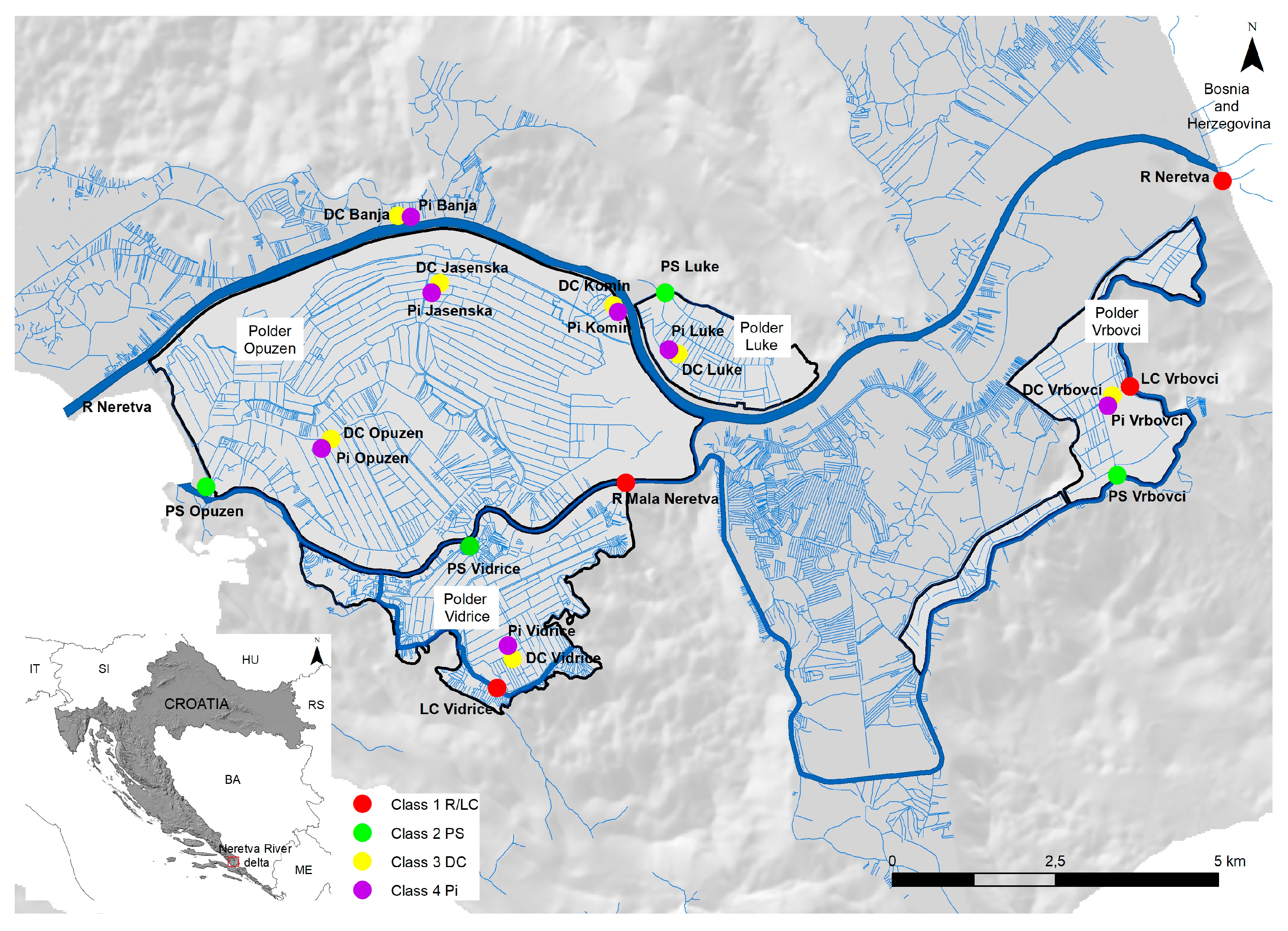
2.1. Study Area Description

The research area is in the NRD, on the southeastern coast of the Adriatic Sea (43°00’ N, 17°30’ E) (Figure 1). The Neretva River is the largest river of the Adriatic catchment area and, according to the annual water discharge, is one of the largest rivers of the Mediterranean Sea [51]. The Neretva River, with its numerous tributaries in its lower course forms an extensive low-lying delta, which influences the main river either directly at the surface or indirectly in the groundwater. The entire delta is under the strong influence of the Adriatic Sea, both through SWI through the main riverbed and groundwater. In the delta, the Neretva River overlies Quaternary deposits. Carbonate rocks, mainly limestone, form the edge of the valley, its flanks, and smaller isolated hill hummocks within the valley [52,53]. These rocks are intensely fractured and deeply karstified. Surface Quaternary sediments consist mainly of peat and clay (organic marshy deposits), which are underlain by clayey sands, sands of variable grain size, sandy clay, gravelly sands, sandy gravel, Holocene gravels (alluvial sediments), and Pleistocene conglomerates. Geomorphology, soil characteristics, and reclamation in the study area are described in detail by Romić et al. [54] and Kralj et al. [55]. Elevations above sea level of individual polders were determined using a digital elevation model (DEM) of the study area. Since the elevation of the polders within the ameliorated area is lower than in the surrounding area, continuous drainage of excess water is required through a dense network of drainage canals, gates, and pumping stations [16]. Polder-like agricultural land is intensively used for the cultivation of citrus fruits and vegetables.

The characterization of the Quaternary aquifer was made by a group of authors [25,56] who compiled the results of a series of hydrogeological, geotechnical, and geophysical studies carried out in the area during the last 60 years (Figure S1). The aquifer system is composed of three main layers. The uppermost layer consists mainly of fine sand with a locally present shallow sublayer of clay and silt. This layer is present throughout the NRD area and represents the unconfined aquifer with a total thickness of 1–10 m. Beneath the unconfined layer a compact clayey-silt layer with a thickness of 10–25 m, which rises slightly towards the sea and forms an aquitard, has been determined. This layer continues below the seabed offshore. Finally, beneath the clay layer is a confined aquifer of mostly coarse gravel with a total depth of 130 m unless bedrock is encountered. The bedrock in this area is karstified limestone, whose depth varies from the ground surface at the edge of the valley to a maximum depth of 165 m below ground level in the middle of the valley [56].

The area is semiarid with a Mediterranean climate, with dry, hot summers and humid, mild winters. The mean annual rainfall for the main weather station of the area (Ploče) is 1077 mm (1988–2020), with most of the rainfall occurring in the period from October to April. The minimum rainfall occurs in July (28 mm) and the maximum occurs in November (153 mm). The mean annual air temperature is 15.9 °C, with January being the coldest (7.0 °C) and July the warmest month (25.7 °C). The annual Penman–Montheith reference evapotranspiration is 1217 mm, with the highest value of 197 mm occurring in July.

2.2. Monitoring Network Design and Data Collection

In the study area, the surface-water- and groundwater-quality monitoring program, established in 2009, has been focused on salinization to identify long-term changes that have both natural and anthropogenic causes and to provide farmers and decision makers with effective data from which to derive information for management and restoration. The monitoring network covers an area of 5815 ha and includes four different polders with surface and groundwater monitoring locations. In addition, surface waters were grouped into classes based on their common characteristics and functions within the polders. Shallow piezometers made of 110 mm diameter plastic pipes with a porous section of 3 to 4 m in length for groundwater monitoring were installed in the central part of each polder. Water samples were collected at several locations within each water class (see Table S1). Water-quality data from the 1 January 2010 to the 31 December 2020 from 15 surface-water bodies (three classes: Class 1 RIVER/LATERAL CANAL, Class 2 PUMPING STATION, and Class 3 DRAINAGE CANAL) and 7 groundwater locations (Class 4 PIEZOMETER) were processed in this study. The water-quality data from 2021 were used to validate the developed forecasting models. The geographical setting of the study, including four polders within the floodplain and the water sampling locations, is shown in Figure 1.

Water samples were collected monthly by direct filling with a hand-held bottle sampler (surface water) and by pipe sampling from piezometers specifically designed for groundwater sampling. Sampling, sample transport, and handling followed a standardized procedure [57,58]. The samples used for the determination of orthophosphate (o-PO₄) were filtered through a membrane filter (0.45 μm mesh size) immediately after sampling. Samples used for the determination of ammonium nitrogen (NH₄-N) were preserved by adding sulfuric acid to adjust the sample to a pH of approximately 2. Water electrical conductivity (EC_w) was measured using a Mettler Toledo MPC conductivity meter with a cell constant control and temperature compensation device (25 °C), according to [59]. pH was determined with a Schott Lab 870 pH meter [60]. Analysis of Cl⁻ and SO₄²⁻, NO₃-N, NH₄-N, and o-PO₄ was performed with a segmented flow system (SFA) and spectrometric detection using a Skalar San+ Analyzer following standard procedures [61,62,63,64], respectively. Determination of sodium and potassium was performed using an AAS PerkinElmer 3110 atomic emission spectrometer following standard procedures [65]. Determination of Ca²⁺ and Mg²⁺ was performed with a Varian VISTA-MPX CCD Simultaneous ICP-OES [66]. The determination of bicarbonates was performed by acid-base titration with H₂SO₄. Data quality-control assurance for water analysis was implemented using a quality system accredited to [67] standard, by using field blank samples, field duplicates, participation in the international proficiency testing program, and internal reference samples.

Monthly mean sea levels were recorded at the tide gauge station located in the Adriatic Sea at the Mala Neretva River mouth, and the data were provided by Croatian Waters (the public water management company in Croatia).

2.3. Statistics

The univariate summary statistics of the variables that describe water chemistry were calculated first. A total of twelve variables were selected (pH, EC_w, Ca²⁺, Mg²⁺, K⁺, Na⁺, HCO₃⁻, Cl⁻, SO₄²⁻, o-PO₄, NO₃-N, and NH₄-N). In addition to summary statistics, one-way analysis of variance (ANOVA) was performed for all variables between the different water classes along with Tukey’s multiple comparison test. Univariate statistical analysis and ANOVA were performed using the statistical software package XLSTAT [68].

2.3.1. Principal Component Analysis

PCA was applied to determine correlations among the variables and to summarize the variation within the data. PCA is a technique for reducing the dimensionality of large data sets, increasing interpretability but at the same time minimizing information loss [69]. PCA involves a mathematical procedure that reduces the variables into major controlling components, thereby enabling the interpretation of variable distributions (common sources of ions and hydrochemical processes). Here, PCA was performed in the R programming language using the FactoMineR package [70].

2.3.2. Time Series and Testing for Stationarity

A time series is a sequence of observations taken sequentially in time [71] and there are several possible objectives in analyzing time series, such as description, explanation, control, and prediction [72]. Stationarity is an important concept in time-series analysis that has a large impact on how data are perceived and predicted. When forecasting or predicting future events, most time-series models assume that each data point is independent of the others (stationary). A time series is said to be strictly stationary if its properties (or the process that generates them) are unaffected by changes in its temporal origin [73]. There are several tests for testing the stationarity properties of time series, and one of the most commonly used is the unit root test proposed by Dickey and Fuller [74]. The null hypothesis of the Dickey–Fuller (DF) test is that there is a unit root in the first-order Autoregressive (AR) model, implying that the data series is not stationary [75]. In the case of higher-order autocorrelation, the Augmented Dickey–Fuller (ADF) test is used to detect the higher-order autocorrelation. If the calculated p-value is below the set significance level, the null hypothesis is rejected, indicating that the series is stationary. If non-stationarity is present in the data, the data must be transformed, often by differencing, i.e., by applying the difference operator to the original time series to obtain a new one [73]. In first order differencing, the difference between consecutive data points is calculated [76] (Equation (1)).

$${\mathrm{y}}_{\mathrm{t}}^{\prime }={\mathrm{y}}_{\mathrm{t}}-{\mathrm{y}}_{\mathrm{t}-1}$$

(1)

2.3.3. Granger Causality Test

The GC test is one of the most robust methods available to detect the causal interactions between two time series and was initially introduced in the field of economics [77,78]. The GC test is a statistical hypothesis test for determining whether one time series is useful for forecasting another. If the probability value is less than any level, then the hypothesis would be rejected at that level. GC addresses the issue with prediction rather than correlation to identify causation between time-series variables [79]. One of the main assumptions of the GC test is the stationarity of the time series. To conduct the analysis, Granger [78] proposed a bivariate model between two time series (Equations (2) and (3)), where X and Y are two stationary time series; a, b, c and d are coefficients; and ε_t η_t are two uncorrelated white-noise series.

$${\mathrm{Y}}_{\mathrm{t}}={\sum }_{\mathrm{j}=1}^{\mathrm{m}}{\mathrm{a}}_{\mathrm{j}}{\mathrm{Y}}_{\mathrm{t}-\mathrm{j}}+{\sum }_{\mathrm{j}=1}^{\mathrm{m}}{\mathrm{b}}_{\mathrm{j}}{\mathrm{X}}_{\mathrm{t}-\mathrm{j}}+{\mathsf{\epsilon }}_{\mathrm{t}}$$

(2)

$${\mathrm{X}}_{\mathrm{t}}={\sum }_{\mathrm{j}=1}^{\mathrm{m}}{\mathrm{c}}_{\mathrm{j}}{\mathrm{X}}_{\mathrm{t}-\mathrm{j}}+{\sum }_{\mathrm{j}=1}^{\mathrm{m}}{\mathrm{d}}_{\mathrm{j}}{\mathrm{Y}}_{\mathrm{t}-\mathrm{j}}+{\mathsf{\eta }}_{\mathrm{t}}$$

(3)

2.3.4. Vector Autoregressive Model

A Univariate Autoregressive (AR) model is a linear model with a single equation and a single variable, in which the current value of a variable is explained by its lagged (previous) values [80]. In the VAR model, on the other hand, there are multiple variables, and each of them is modelled as a linear combination of the lagged values of itself and the lagged values of the other variables in the system. It represents an extension of the univariate AR model to dynamic multivariate time series and was proposed by Sims [81]. For a set of K time-series variables y_t = (y_1t, …, y_Kt)’, a VAR model captures their dynamic interaction. The basic p-lag VAR model is of the following form (Equation (4)).

$${\mathrm{y}}_{\mathrm{t}}={\mathrm{A}}_1{\mathrm{y}}_{\mathrm{t}-1}+...+{\mathrm{A}}_{\mathrm{p}}{\mathrm{y}}_{\mathrm{t}-\mathrm{p}}+{\mathsf{\epsilon }}_{\mathrm{t}}$$

(4)

where A_i’s (K × K) are coefficient matrices and ε_t is an unobservable error term [82]. One of the advantages of the VAR model is that it does not require as much knowledge about a variable affecting the factors but rather a list of variables that are assumed to interact intertemporally [83]. The lag length for the VAR(p) model may be determined using model selection criteria. The general approach is to fit VAR(p) models with orders p = 0, ..., pmax and to choose the value of p that minimizes some model selection criteria. The three most common information criteria are the Akaike (AIC), Schwarz–Bayesian (BIC), and Hannan–Quinn (HQ) criteria [84].

2.3.5. Model Performance Assessment

Many different criteria, such as the coefficient of determination (R²), mean square error (MSE), sum of square errors (SSE), root mean square error (RMSE), mean absolute error (MAE), and many others, are used by authors to evaluate the performance of developed statistical models [85]. The coefficient of determination (R²) is a statistical tool that helps in identifying the relationship between variables in a regression model and represents a measure of the proportion of explained variance present in the data [86]. Low values of R² (<0.5) indicate a weak relation between the predictor variables and the response variables. The calculation of R² is as follows:

$${\mathrm{R}}^2=1-\frac{\sum ({{\mathrm{y}}_{\mathrm{i}}-\widehat{\mathrm{y}})}^2}{\sum ({{\mathrm{y}}_{\mathrm{i}}-\stackrel{-}{\mathrm{y}})}^2}$$

(5)

The root mean square error (RMSE) is used to calculate the standard deviation of the residuals between the observed and predicted data values [87]. Whereas R² is a relative measure of fit, RMSE is an absolute measure of fit, and lower values indicate better fit [88]. It is calculated as follows:

$$\mathrm{R}\mathrm{M}\mathrm{S}\mathrm{E}=\sqrt{\frac{1}{\mathrm{n}}\mathrm{\ast }{\sum }_{\mathrm{i}=1}^{\mathrm{n}}{\left({\mathrm{y}}_{\mathrm{i}}-\widehat{\mathrm{y}}\right)}^2}$$

(6)

Mean absolute error (MAE) represents the average of the absolute difference between observed and predicted values and is often used to measure the prediction error in time-series analysis [87]. It is calculated as follows:

$$\mathrm{M}\mathrm{A}\mathrm{E}=\frac{1}{\mathrm{n}}\mathrm{\ast }{\sum }_{\mathrm{i}=1}^{\mathrm{n}}|{\mathrm{y}}_{\mathrm{i}}-\widehat{\mathrm{y}}|$$

(7)

Sum of square error (SSE) represents the difference between the observed and predicted value (Equation (8)) while the mean square error (MSE) represents the average of the squared difference between the observed and predicted data (Equation (9)).

$$\mathrm{S}\mathrm{S}\mathrm{E}={\sum }_{\mathrm{i}=1}^{\mathrm{n}}{({\mathrm{y}}_{\mathrm{i}}-\widehat{\mathrm{y}})}^2$$

(8)

$$\mathrm{M}\mathrm{S}\mathrm{E}=\frac{1}{\mathrm{n}}\mathrm{\ast }{\sum }_{\mathrm{i}=1}^{\mathrm{n}}{({\mathrm{y}}_{\mathrm{i}}-\widehat{\mathrm{y}})}^2$$

(9)

PCA, ADF tests, GC tests, and VAR models were performed using R statistical software [89].

3. Results

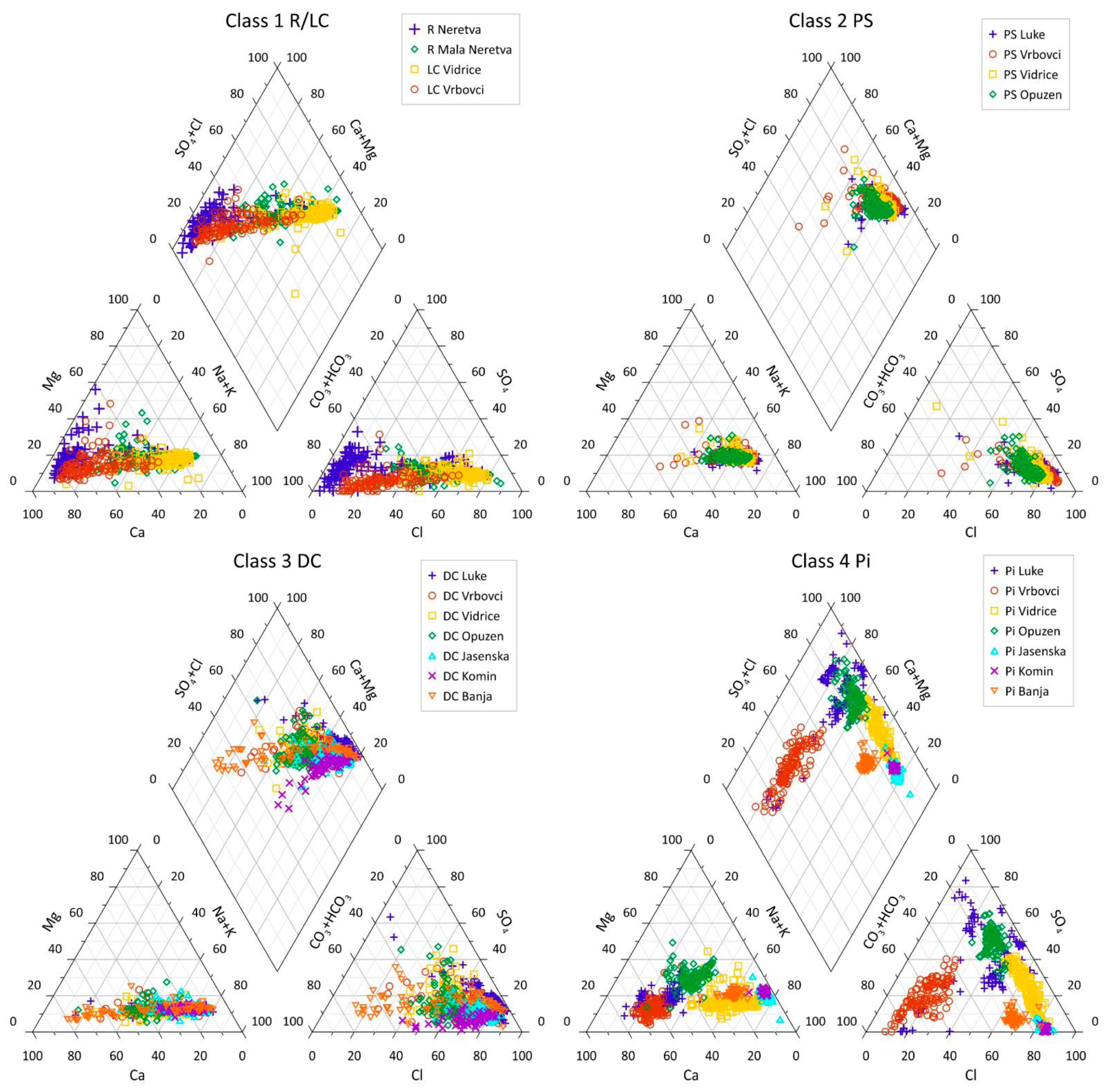
3.1. Surface-Water and Groundwater Chemistry

In this study, three classes of surface-water bodies were defined in terms of their common characteristics and using two categories of indicators: (1) natural state or/and extent of modification and (2) hydrological functions of the water body within the polder-type agricultural catchment. Piezometers representing the groundwater body are installed in each polder in the NRD to (1) assess the impact of agricultural practices on groundwater and (2) assess the impact of saline groundwater on the salinization of soil and consequently on agricultural crops. Descriptive statistics on the chemistry of the water bodies divided into classes, as shown in

Table 1. Descriptive statistics (means, minima, maxima, and standard deviations) and results of analysis of variance (ANOVA) with Tukey’s honestly significant difference (HSD) test for twelve water-quality parameters for each water class.

Class	Desc. Statistics	Parameters
		pH	ECw	Ca2+	Mg2+	K+	Na+	HCO3−	Cl−	SO42−	o-PO4	NO3-N	NH4-N
			dS m−1	mg L−1
1 River/Lateral Canal (R/LC)	N	528	528	528	528	528	528	528	528	528	528	528	528
	Mean	7.83	1.05	84.6	24.1	5.66	113	251	222	53.5	0.03	0.26	0.65
	Median	7.84	0.8	84.9	19.4	4.60	74.2	250	141	46.3	0.01	0.02	0.66
	Min.	7.14	0.26	52.9	2.92	0.40	1.90	168	3.21	0.50	0.01	0.01	0.01
	Max.	8.46	3.77	136	87.5	22.1	564	332	1674	299	0.30	6.97	2.09
	St. dev.	0.18	0.68	13.1	16.4	4.48	113	32.8	229	38.4	0.05	0.41	0.29
2 Pumping Station (PS)	N	528	528	528	528	528	528	528	528	528	528	528	528
	Mean	7.65	4.02	146	96.8	24.0	599	316	1181	247	0.04	0.55	0.78
	Median	7.67	3.71	141	89.0	22.7	554	311	1080	225	0.03	0.19	0.74
	Min.	7.10	0.71	72.1	13.6	2.20	44.5	214	46.1	29.4	0.01	0.01	0.03
	Max.	8.43	12.2	513	350	73.6	2120	610	4035	814	0.30	13.7	3.24
	St. dev.	0.17	1.51	46.0	39.7	9.03	268	52.4	538	117	0.04	1.10	0.41
3 Drainage Canal (DC)	N	800	800	800	800	800	800	800	800	800	800	800	800
	Mean	7.61	3.82	160	92.2	22.3	565	334	1085	289	0.05	0.60	0.83
	Median	7.64	3.01	128	71.9	17.2	397	305	779	185	0.03	0.13	0.74
	Min.	6.70	0.19	44.9	6.67	0.50	12.0	107	10.9	16.6	0.01	0.01	0.01
	Max.	8.38	36.3	830	886	245	7469	775	13125	2674	1.00	29.5	5.32
	St. dev.	0.22	3.45	106	84.4	20.4	632	97.6	1170	332	0.07	1.83	0.53
4 Piezometer (Pi)	N	770	770	770	770	770	770	770	770	770	770	770	770
	Mean	7.55	10.7	331	324	101	1883	1222	3485	757	1.20	7.70	23.5
	Median	7.57	6.70	305	242	78.9	779	671	1297	460	0.06	1.38	2.75
	Min.	6.40	0.29	33.7	3.89	6.00	7.60	39.7	13.9	0.50	0.01	0.01	0.01
	Ma.	8.57	38.9	978	1439	321	7700	3965	19498	3098	12.0	102	175
	St. dev.	0.24	10.2	184	297	84.0	2194	1072	4157	716	2.47	16.0	40.6
ANOVA (Summary of all pairwise comparisons for Class (Tukey (HSD)):
R/LC	Groups	A	A	A	A	A	A	A	A	A	A	A	A
PS		B	B	B	B	B	B	A	B	B	A	A	A
DC		C	B	B	B	B	B	A	B	B	A	A	A
Pi		D	C	C	C	C	C	B	C	C	B	B	B

, clearly indicate different environmental influences.

Different water types can be distinguished based on their ion composition. Figure 2 provides a visual representation of the balance between different cations (positively charged ions) and anions (negatively charged ions) in water. The Piper diagram (Figure 2) clearly identifies various hydrochemical facies that reflect the response of chemical processes and the pattern of the water bodies’ interconnection.

Water bodies belonging to the Class 1 RIVER/LATERAL CANAL (R/LC) were supposed to reflect natural conditions and were mostly unaffected by anthropogenic pressures, although they were considered pristine reference waterbodies. The Class 1 R/LC water bodies are fed freshwater from the catchment. They are least affected by saline water intrusion and are low in nutrients (Table 1). The order of the main cation mean concentrations was Na⁺ > Ca²⁺ > Mg²⁺ > K⁺, and their concentrations were significantly lower than those in the other water-body classes. Maximum concentrations of all cations and anions except nutrients (N species) indicate the periodical intrusion of the saline water into the river courses, which has been obviously modifying the natural state common for the river water composition, particularly in Class 1 LC Vidrice and R Mala Neretva, which are located closest to the sea (Figure 1).

Class 2 and Class 3 water bodies exhibit similar physicochemical characteristics, which are highly affected by hydrological changes due to technical maintenance of the polder-type floodplain. The mean electrical conductivity values (EC_w) at Class 2 PUMPING STATION (PS) and in Class 3 DRAINAGE CANAL (DC) were higher than those of the Class 1 water bodies. Although the mean EC_w values of Class 2 PS and Class 3 DC water bodies did not differ substantially, the range of EC_w was much wider in the DC, reaching 36 dS m⁻¹ in certain periods of the year. The order of the main cation mean concentrations did not differ compared to all classes in the water of Classes 2 and 3, being Na⁺ > Ca²⁺ > Mg²⁺ > K⁺. Mean nutrient concentrations were low, and the highest maximum concentrations of nitrate and ammonium were recorded in drainage canals.

Class 4 PIEZOMETER (Pi) exhibited distinctively different hydrochemistry compared to the classes of the surface-water bodies. As a result of periodic intense SWI into coastal aquifers, the mean EC_w value was the highest (10.7 dS m⁻¹) and significantly different from the surface-water classes. The range of EC_w values in groundwater was similar to the range for the same parameter in Class 3 DC, but the mean was significantly higher (11 dS m⁻¹). Class 3 DC water bodies showed similar EC_w value ranges, but with distinctively lower mean values, which indicated hydrological connectivity between surface water and groundwater. The mean concentrations of the main cations were significantly higher in Class 4 Pi than in the surface-water classes, but the order of the main cation mean concentrations was still the same: Na⁺ > Ca²⁺ > Mg²⁺ > K⁺. The maximum EC_w value was 38.9 dS m⁻¹, which was close to the seawater salinity level. Obviously, all water bodies in the study area have been impacted by increasing EC_w.

ANOVA showed that pH differed significantly among all classes of water bodies (Table 1). The main cation concentrations in Class 1 R/LC water bodies differed significantly from those in Class 2 PS and Class 3 DC, which did not differ. The nutrient concentrations were not significantly different in the surface-water bodies but were significantly different from the nutrient concentrations in the groundwater. The significant difference in ion composition between all surface-water bodies and groundwater was confirmed by the analysis of variance (Table 1).

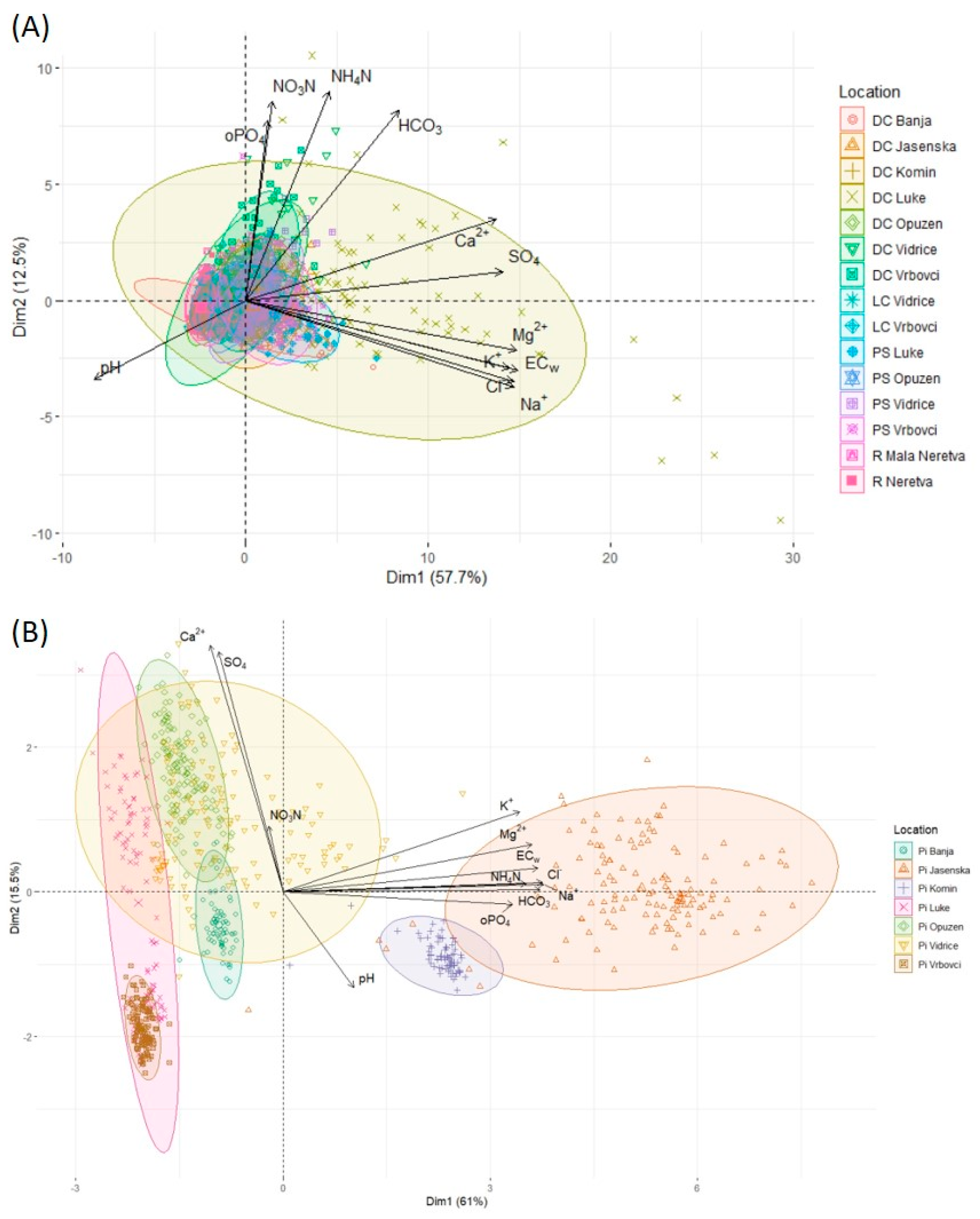
3.2. Multivariate Statistics

As shown in Figures S2–S4, PCA was performed on hydrochemical variables for all classes of surface water as well as for every class of surface water separately. Most of the variation for all classes is explained by the first two principal components, which cumulatively explained more than 70% of the variation in surface-water bodies, and more than 76% in groundwater (

Table 2. Principal component analysis of surface-water bodies (including all three classes) and groundwater—eigenvalues, variance (%), and cumulative variance (%) for the first three principal components.

Surface Water
Principal component	Eigenvalue	Variance (%)	Cumulative variance (%)
PCOMP 1	6.92	57.6	57.6
PCOMP 2	1.49	12.5	70.1
PCOMP 3	1.02	8.47	78.6
Groundwater
Principal component	Eigenvalue	Variance (%)	Cumulative variance (%)
PCOMP 1	7.32	61.0	61.0
PCOMP 2	1.85	15.5	76.5
PCOMP 3	1.03	8.62	85.1

). Even though the water bodies were grouped into classes based on their common hydrological features, not all of them contributed equally to the dominant patterns of ion species identified by PCA (Figure 3).

The PCA results for all surface-water bodies analyzed jointly indicate that the most relevant variables in all water classes (i.e., the ones that explain most of the variance) are EC_w, Na⁺, Ca²⁺, Cl⁻, Mg²⁺, K⁺, and SO₄²⁻, which are related to the SWI. In this context, water salinization may be assigned as a dominant process, explaining 57.6% of the total variance (Table 2). Nutrient loadings to the surface waters (NO₃-N, NH₄-N, and o-PO₄) were evident as well (Figure 3A), and they explain 12.5% of the variance in the second component, reflecting direct anthropogenic pressure deriving from agricultural activities. Nevertheless, due to differences in agricultural management practices in the polders, not all surface-water bodies contributed equally to both principal components.

As shown in Figure 3A, which presents a PCA biplot for surface-water bodies, the highest contribution to water salinity belongs to the DC Luke, located in the polder that receives a large amount of groundwater seepage, while the drainage canals and pumping stations collect and transfer most of the nutrients leached from the agricultural fields. The PCA variable contributions for each surface-water class are given separately in Table S2, and related PCA biplots are shown in Figures S2–S4. Visual comparison of the biplots and analysis of clusters of the same observations in different classes of surface-water bodies shows distinct patterns for the contribution of ions, which are confirmed by the variable contribution indices shown in Table S2.

In the case of Class 1 R/LC, the locations closest to the sea, which are R Mala Neretva and LC Vidrice, contribute most to the water salinity, explaining 46.5% of the variance by the first component. Major variable contributions in the first PCA dimension come from EC_w, Mg²⁺, K⁺, Na⁺, Cl⁻, and SO₄²⁻. The dominant process affecting water chemistry identified in the second component is the freshwater inflow through the main river course and lateral canals. Major variable contributions in the second PCA dimension come from pH, EC_w, Ca²⁺, K⁺, and HCO₃⁻. The contribution of nutrient loadings is rather low, scattered unevenly within the third, fourth, and fifth dimensions, going in the opposite direction of the two main driving forces (Figure S2). This phenomenon is related to the intrinsic character of the streams grouped in Class 1 R/LC. Numerous tributaries influence the main river stream, either directly on the surface or indirectly in groundwater, and drain mountains of Bosnia and Hercegovina built of magmatic, metamorphic, carbonate, and clastic sedimentary rocks.

In contrast, surface-water bodies of Class 2 PS and Class 3 DC contribute the most to the nutrient loadings. The contribution of nutrient concentrations in surface-water classes is scattered unevenly among the second to the fifth components (Table S3). However, the share of contribution to the nutrient loadings among the surface-water classes suggests several sources and possibly different intensities of NO₃-N, NH₄-N, and o-PO₄ fluxes within the floodplain. The highest loading of nutrients is attributed to the water bodies at the pumping stations. Among Class 3 DC, Luke exhibits the highest salinity for drainage water, while DC Jasenska, DC Vidrice, and DC Vrbovci drain mostly nutrients. Obviously, differences in the agricultural land use of polders and dominant crop production result in unequal water chemistry and the prevailing contributions of specific ions, particularly nutrients.

Class 2 PS cluster water bodies are supplied by pumping stations within the polders in the process of maintaining the groundwater table and the water level in the canals. Visual inspection of the biplot presented in Figure S3 shows an even contribution to the nutrient loadings of all monitoring locations belonging to Class 2 PS but a more pronounced impact of PS Luke on the water salinity. For all surface-water classes, PCA recorded a similar contribution of nutrient loadings to the water chemical composition, although the specific variable contributions in the third, fourth, and fifth dimensions indicate different nutrient sources and/or flow paths.

The highest contribution of DC Luke to the salinity of Class 3 DC is evident from the biplot shown in Figure S4. Along with DC Vidrice, the same location highly contributes to the nutrient loadings. The surface elevation of the polder Luke located on the right side of the Neretva River varies between −3.04 and 0.63 m above sea level. Land surface elevation is the highest on the river embankments and fluvial terraces along the main water courses, decreasing toward the former swamp area. In this polder, land subsidence is the most pronounced, which further accelerates groundwater seepage and impacts surface-water quality. Unlike other polders, where saline water intrudes into groundwater through the karstified aquifer, water salinization in Luke derives from the salt wedge in the Neretva River. However, the flow pattern and intensity of salinization of the water in this polder depend on the dynamics of the pumping station operation and obviously increase with the pumping of excess water.

The PCA biplot of Class 4 Pi (Figure 3B) shows a clear distinction in groundwater chemistry among monitoring locations. The first principal component that explains 61% of the variance is evidently related to the water salinity, most pronounced in Pi Jasenska, as shown in Table S4. This polder was developed by the reclamation of the salt lake, and the location obviously communicates with the sea even at present. The only partial overlapping with the Pi Jasenska was observed for Pi Komin, located at the edge of the former lake.

3.3. Time-Series Analysis

3.3.1. Augmented Dickey–Fuller Test

An ADF test is performed before developing time-series models, and the p-values for each site and water-quality parameter are given in Table S5. In all surface-water classes (R/LC, PS, and DC), the time series for variables related to seawater, i.e., EC_w and all major ions, are stationary, except for Cl⁻ at DC Vidrice (p-value = 0.07) and SO₄²⁻ at R Neretva (p-value = 0.23), which are non-stationary. Non-stationarity in the surface-water classes was observed mainly in the time series for nutrients, with the highest p-values observed for o-PO₄ at R Neretva (0.38), LC Vidrice (0.46), LC Vrbovci (0.55), and PS Luke (0.44), and the highest p-values for NH₄-N at DC Komin (0.31) and DC Banja (0.53). The results of the ADF test for the groundwater Class 4 Pi, as shown in Table S5, are more complex and are unevenly scattered both among locations and among parameters at individual locations. According to the ADF test, only the time series for pH at each location within the Pi water class are stationary. At Pi Luke, the time series for all variables except NH₄-N are non-stationary, in addition to the low p-values for the other two nutrients, o-PO₄ (0.06) and NO₃-N (0.09). In addition, the parameters related to salinity are non-stationary, due to the salinization processes deriving from the salt wedge in the main riverbed of the Neretva River, which is seasonally affected by both river inflow and SWI. Only at two sites, Pi Jasenska and Pi Vidrice, are the EC_w time series stationary (Table S5). In addition to the EC_w time series being stationary, the time series for ions closely related to water salinity are also either stationary at both locations (Mg²⁺, Cl⁻, and HCO₃⁻) or have p-values very close to alpha of 0.05 (Na⁺ and K⁺ at Pi Jasenska). Polders Vidrice (where Pi Vidrice was installed) and polder Opuzen (where Pi Jasenska was installed) are located closest to the Adriatic Sea and have low mean elevations of −0.44 m a.s.l. and −1.13 m a.s.l., respectively. Since the stationarity of the time series is one of the prerequisites for the development of forecast models, all non-stationary time series were transformed to stationary ones by differencing.

3.3.2. Granger Causality

As we studied the hydrological response of sea-level fluctuation on water salinity within the polders, the GC test was applied to assess whether one time series is useful in forecasting another, i.e., whether one variable at time t-lag causes another variable at time t.

Table 3. Results for the Granger causality test when EC_w is considered as an effect and sea levels as possible causes for selected water classes (RIVER/LATERAL CANAL and PIEZOMETER).

Water Class	Location	F-Statistic	p-Value	Accept/Reject
River (R)/Lateral Canal (LC)	R Neretva	1.509	0.146	Accept
	R Mala Neretva	8.288	2.84 × 10-5	Reject
	LC Vidrice	5.308	0.001	Reject
	LC Vrbovci	1.522	0.184	Accept
Piezometer (Pi)	Pi Opuzen	0.021	0.989	Accept
	Pi Vidrice	7.380	9.376 × 10-5	Reject
	Pi Jasenska	3.039	0.030	Reject
	Pi Vrbovci	1.986	0.097	Accept
	Pi Komin	0.691	0.559	Accept
	Pi Banja	0.761	0.518	Accept

shows p-values for the GC test when water salinity (EC_w) is considered as the effect and sea levels are considered as possible causes. We presumed that Class 3 DC and Class 2 PS are under the dominant influence of the polder maintenance system (i.e., pumping station operation dynamics), so we excluded these classes from the GC testing. The GC test was performed on groundwater and water bodies of the Class 1 R/LC to identify and describe the hydrological effect of sea-level fluctuation on groundwater and surface-water salinity caused by direct SWI into aquifers. As already mentioned, in polder Luke, water salinization derives from the salt wedge in the River Neretva, and therefore this location was excluded from the GC test. The null hypothesis was that there is no GC between the cause and the effect and that the lower the p-value is, the stronger the causality. The results presented in Table 3 show that there is a strong causal relationship between sea level and water salinity only at two locations of class 1 R/LC (R Mala Neretva and LC Vidrice) and at two locations of Class 4 Pi (Pi Jasenska and Pi Vidrice). R Mala Neretva and Pi Jasenska are located in polder Opuzen, which has the lowest individual point elevation of −4.05 m a.s.l. and an average elevation of −1.13 m a.s.l. The polder Vidrice, where LC Vidrice and Pi Vidrice are located, has a mean elevation of −0.44 m a.s.l., and the lowest point is −2.61 m a.s.l. Moreover, these two polders are closest to the Adriatic Sea, which may explain the causal relationship between the water salinity and the sea level.

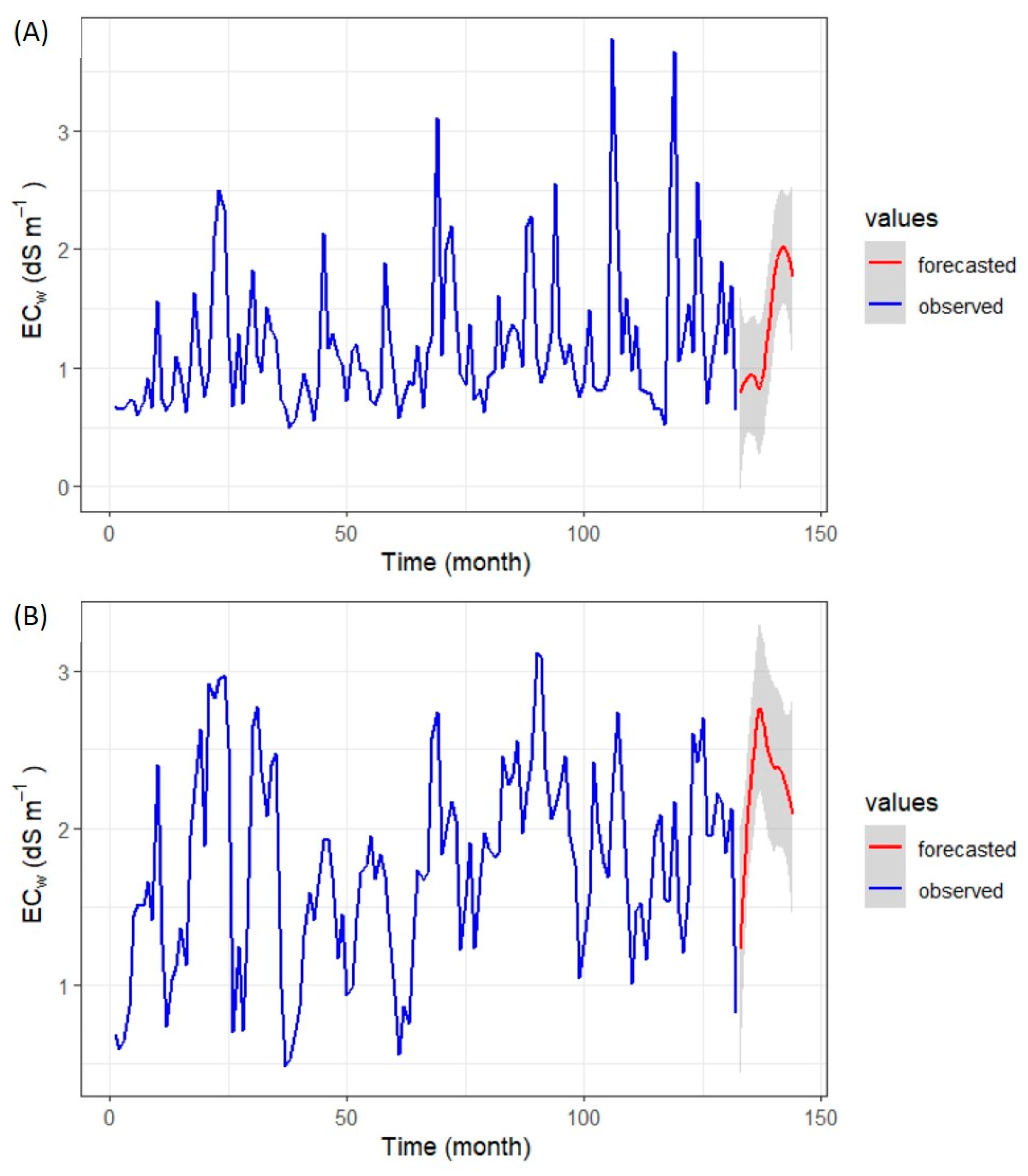
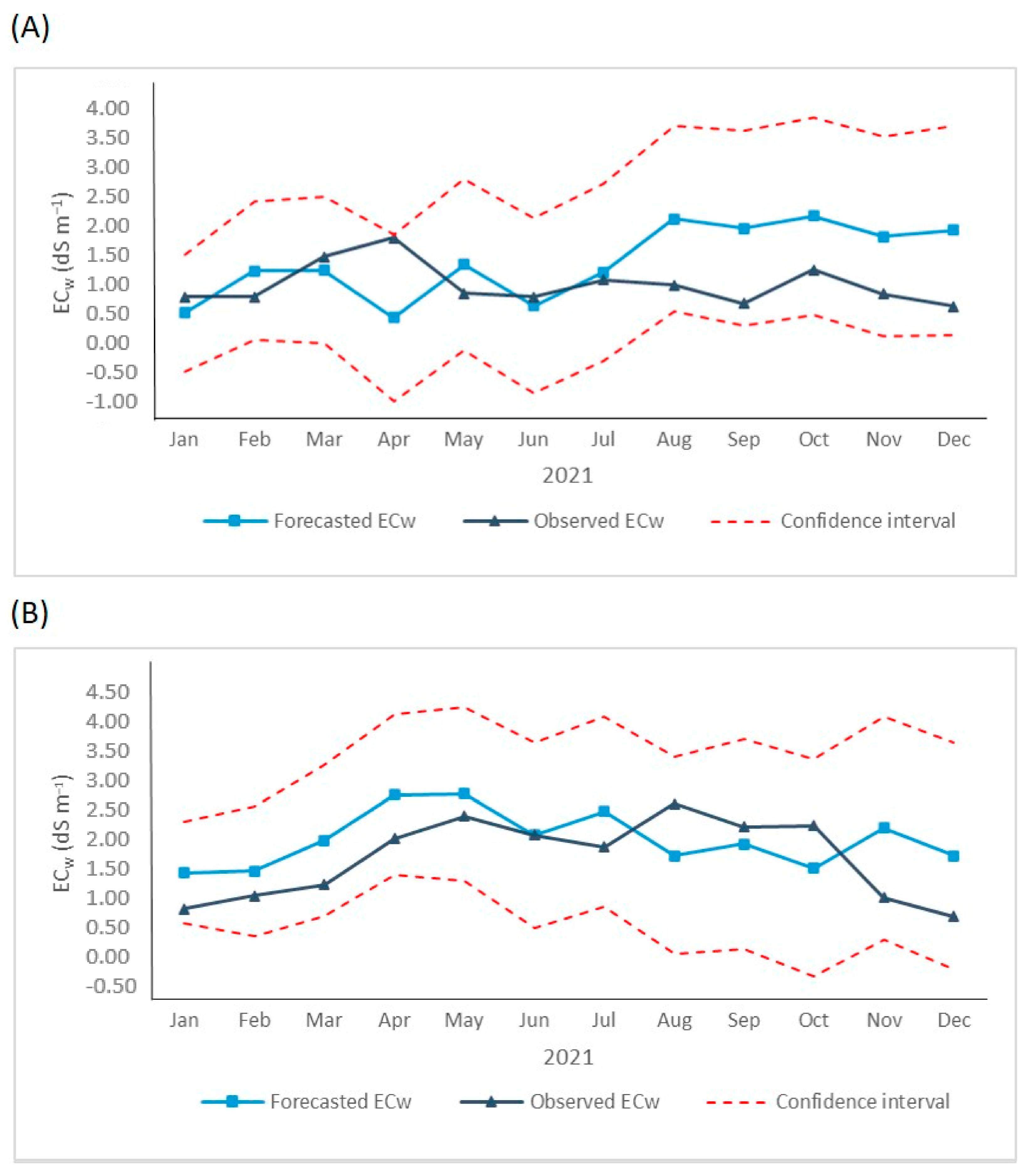
3.3.3. Forecasting Based on the Vector Autoregressive Model

The VAR model is a multivariate time-series model used to examine the dynamic relationship between two or more variables that interact with each other, where each variable is modelled as a linear combination of the lagged value of both itself and the lagged values of other variables in the system. VAR models were developed for four locations that showed causal relationships with the GC test, Class 1 R/LC R Mala Neretva and LC Vidirce as surface-water bodies and Class 4 Pi Jasenska and Pi Vidrce as groundwater bodies. Nine endogenous variables associated with SWI were selected: pH, EC_w, Ca²⁺, Mg²⁺, K⁺, Na⁺, HCO₃⁻, Cl⁻, and SO₄²⁻. The maximum number of lags was determined using the AIC. R² was used to evaluate how well the developed models fit the observed data.

The results show that the VAR models developed for both Class 1 R/LC locations for pH, EC_w, Ca²⁺, and HCO₃⁻ and for K⁺ for LC Vidrice have R² values greater than 0.9, indicating that they fit the observed data well (

Table 4. Results of VAR model performance (R²) for two surface-water and groundwater locations selected with the Granger causality test.

Variables	Surface Water		Groundwater
	LC Vidrice	R Mala Neretva	Pi Vidrice	Pi Jasenska
	R2	R2	R2	R2
pH	0.999	0.999	0.330	0.167
ECw	0.947	0.932	0.220	0.095
Ca2+	0.976	0.991	0.532	0.271
Mg2+	0.790	0.804	0.496	0.241
K+	0.931	0.784	0.224	0.126
Na+	0.715	0.735	0.350	0.102
HCO3−	0.954	0.997	0.464	0.120
Cl−	0.718	0.754	0.361	0.193
SO42−	0.504	0.666	0.397	0.170

). The models for Mg²⁺, Na⁺, and Cl⁻ for both locations and for K⁺ for R Mala Neretva have R² values between 0.6 and 0.8, and only the model for SO₄²⁻ at LC Vidrice has a value below 0.6 and explains only 50% of the variability of the fitted data. In general, the VAR models developed for two Class 1 R/LC locations explain more than 60% of the variability in the observed variables for all parameters except SO₄²⁻ at LC Vidrice and can therefore be used for reliable forecasting. The results of the VAR models for the two Class 4 Pi locations Pi Vidrice and Pi Jasenska differ significantly from those for Class 1 R/LC. None of the developed VAR models for forecasting any of the nine variables have R² values higher than 0.53 (Table 4). At Pi Jasenska, all models have a very low R² value, and only the models for Ca²⁺ and Mg²⁺ have R² values higher than 0.2. At Pi Vidrice, the VAR models for Mg²⁺ and Ca²⁺ have the highest R² values, 0.50 and 0.53, respectively (Table 4). Consequently, none of the developed VAR models could provide reliable predictions for Class 4 Pi locations Pi Vidrice and Pi Jasenska; therefore, only the surface-water Class 1 locations LC Vidrice and R Mala Neretva were selected for forecasting.

Forecasts for EC_w based on the VAR model with monthly granularity for one year (2021) ahead were made. Figure 4A shows the forecast for EC_w for 2021 at Class 1 R/LC location R Mala Neretva. The forecasted EC_w values for 2021 varied from 0.48 dS m⁻¹ in April to 2.09 dS m⁻¹ in October, with a mean value of 1.36 dS m⁻¹ (

Table 5. Monthly observed and forecasted values for EC_w with confidence intervals and calculated RMSEs at R Mala Neretva and LC Vidrice for 2021.

Month	ECw at R Mala Neretva				ECw at LC Vidrice
	dS m−1				dS m−1
	Observed	Forecasted	Confidence Interval	RMSE	Observed	Forecasted	Confidence Interval	RMSE
Jan	0.81	0.55	0.92	0.8	0.82	1.39	0.80	0.66
Feb	0.80	1.22	1.09		1.02	1.41	1.03
Mar	1.45	1.23	1.15		1.20	1.90	1.19
Apr	1.75	0.48	1.32		1.92	2.61	1.27
May	0.86	1.32	1.36		2.28	2.63	1.37
Jun	0.80	0.67	1.39		1.99	1.98	1.47
Jul	1.07	1.20	1.41		1.80	2.35	1.50
Aug	0.99	2.04	1.47		2.48	1.66	1.56
Sept	0.70	1.89	1.54		2.11	1.85	1.66
Oct	1.23	2.09	1.56		2.13	1.46	1.72
Nov	0.86	1.77	1.58		0.99	2.10	1.76
Dec	0.65	1.86	1.65		0.70	1.66	1.79

). The average value of EC_w for the eleven-year period (2010–2020) was 1.18 dS m⁻¹. Figure 4B shows the forecast for EC_w for 2021 at the Class 1 R/LC location LC Vidrice. The forecasted minimum EC_w for 2021 was 1.39 dS m⁻¹ (January) and the maximum of 2.63 dS m⁻¹ was for May (Table 5). The forecasted annual mean was 1.92 dS m⁻¹, which corresponds to the eleven-year average at this location (1.75 dS m⁻¹). The forecasted values of EC_w and confidence intervals are given in Table 5. The results show that it is possible to develop reliable short-term (1-year-ahead) forecasts of water salinity at two Class 1 R/LC locations within the NRD that are very important not only for managing the system but also for planning agricultural production. Indeed, these two locations, the watercourses R Mala Neretva and LC Vidrice, whose main purpose is to protect the area from flooding, also have an important function as major sources of freshwater needed for irrigation of agricultural crops in polders Opuzen (where R Mala Neretva is located) and Vidrice (where LC Vidrice is located), which together cover an area of over 3000 ha, representing more than half of the agricultural area of the NRD.

Model validation is an important part of multivariate data analysis. Model validation is used to compare model predictions with the observed and unknown data set to assess model accuracy and predictive ability [90,91]. The observed EC_w data from 2021 were plotted with forecasted data for 2021, including confidence intervals at the Class 1 R/LC locations R Mala Neretva (Figure 5A) and LC Vidrice (Figure 5B). Visually, all observed and predicted data points at both locations fall between the lower and upper bounds of the confidence interval. To check the goodness of fit of the model, RMSE values were calculated. The calculated RMSE was 0.8 dS m⁻¹ (Table 5) at Class 1 R/LC location R Mala Neretva and 0.66 dS m⁻¹ at LC Vidrice.

4. Discussion

In this study, time series of hydrochemical data of the polder-type agricultural floodplain within the NRD were used to interpret the temporal changes in water salinity and to develop and test the short-term forecasting model needed to assist in optimizing water management decisions. The most specific features of the terrain in the study area comprise the lower-lying parcels of predominantly polder-type land formed in the past by intensive land reclamation and hydro-technical interventions. The complex land reclamation projects in the study area have been intended to ensure flood protection in the rainy season with dikes along the Neretva River. On the Mala Neretva River and at the “mouth” into the sea, sluice gates have been constructed to regulate the flow of high waters and prevent SWI into the local waters of the Mala Neretva during the irrigation season. Maintaining the appropriate regime of flow in drainage canals is directly related to the groundwater level. Low land elevations (partly even below sea level) and shallow groundwater levels require the application of permanent pumping to prevent flooding polders. Such hydrological interventions foster water and solute flow, and hydrologic models provide valuable information for identifying problems and supporting decisions [92]. Due to disparate characteristics, stressor combinations, scales, and management practices, no conceptual methodologies for analyzing linked groundwater–surface-water interactions in a lowland catchment have been developed to date [93]. Groundwater and surface water are not separate components of the hydrological system. Rather, they are linked and interact across a wide range of physiographic and catchment settings, and the exchange of water between streams and shallow groundwater may influence the hydrochemistry in both directions.

4.1. Water Salinization Patterns

Human alterations to flow paths, such as ditches, drainage canals, and similar features in the polder-type floodplain, are aimed at increasing drainage efficiency. However, the natural paths of water and solute flow through the floodplain can be modified, as confirmed by the PCA results. Similar to the results of Li et al. [39], which clearly showed surface hydrological connectivity across the floodplain that resulted in an enhanced spatial similarity in the water quality of the seasonal floodplain lakes, we also found such similarity in terms of a range of water-quality parameters, primarily those related to salinity. This arises from the polders’ flooding control and water pumping system.

Although the region has been extensively studied, none of the previous studies have attempted to analyze the nature of spatial and temporal variations in hydrochemical characteristics in a connected system of water bodies in an artificially managed polder-type floodplain of the NRD. As an ultimate 280 km² segment of a more than 10,000 km² catchment of the Neretva River strikingly different from the rest of the catchment in many features, geological and hydrogeological, the Neretva River itself has been modified through the construction of in-stream hydropower plants and reservoirs. The study of Kralj et al. [55] explained the nature of depositional conditions recorded in Neretva River sediment cores, which are certainly influenced by long-lasting human activity in the whole catchment area. Hydroelectric dams and water-storage structures have changed the historical discharge regime and contributed to sediment deficit in the deltaic part of the river, causing changes in river morphology and ecology.

Romić et al. [16] applied two linear mixed-effects models for the prediction of electrical conductivity and nitrate concentration in the surface waters and groundwater in the NRD. The model was proven to be useful to alert for water-salinization risk due to natural processes. In contrast, the prediction of nitrate concentration in the water was not equally satisfactory, apparently stemming from the heterogeneity of the land management and agricultural practices. In our research, we were further focused on the temporal patterns of surface-water and groundwater salinization induced by both natural processes and human activities.

In terms of food security, ensuring a safe water supply for agriculture in terms of both quantity and quality is the foremost objective in integrated water management. The estuary mouth empties into the Adriatic Sea in the Neretva Channel. Water inflow from the wide catchment spread of over 10,000 km² reaching this point, along with the small streams and springs on the karst edges, is fresh and constant but seasonally variant. In the summer months, when the freshwater inflow is low, seawater enters the riverbed and forms a seawater wedge that can reach more than 20 km upstream from the river mouth (at the town of Metković on the Croatian–Bosnian border). On the other hand, if the freshwater inflow from the catchment area is higher, the salt wedge is pushed downstream. Changes in river flow control salt-wedge dynamics. The spatiotemporal patterns of the extent of the salt wedge and stratification studied by Ljubenkov and Vranješ [94] showed that saline water reaches the border 20 km upstream at a freshwater inflow of less than 180 m³ s⁻¹, while it is completely displaced from the riverbed at an inflow of more than 500 m³ s⁻¹. In other words, the Neretva River is highly stratified, i.e., the freshwater flows above the seawater wedge with a very narrow transition zone (approximately 0.5 m). The balance of input from tidally driven seawater and river inflows that sets up stratification patterns becomes highly disturbed by the water pumping within the polders.

4.2. Water Hydrochemistry and PCA Analysis

Different water bodies or classes of surface waters and groundwater tend to develop distinct hydrochemical characteristics depending on the dynamic mixing of water from different sources [16]. The SWI intensity and seasonal dynamics as well as the water chemistry of surface-water bodies are related predominantly to the inflows from the river catchment. As a narrow delta-shaped riverine estuary, the area is morphologically complex due to the highly transient patterns of river inputs and hydrological connectivity within the different types of water bodies. Hydrochemical changes in various surface-water bodies, such as different types of drainage canals, are induced by more complex processes activated primarily by the pumping-station operation regime that maintains the water table within the polder area. Exfiltration of shallow saline groundwater to prevent the water table from accumulating water from drainage canals may adversely affect the quality of surface water used for irrigation and threaten crop production [95].

The hydrochemistry of surface-water bodies analyzed together by PCA is dominantly affected by the SWI. However, hydrological processes differ among both different surface-water classes and distinct locations within each class. Patterns of water salinization in low-elevation land are highly dynamic, with large variations over not only seasonal but also diurnal timescales due to pumping-station operations [96]. According to the classification of Geyer et al. [97], the NRD is a typical salt-wedge estuary due to its microtidal environment and high freshwater flow rates [98]. As a result of the low tidal dynamics of the Adriatic Sea, where mean tidal amplitudes do not exceed 30 cm [99], the Neretva River is highly stratified, which means that freshwater flows above the seawater wedge. Groundwater salinization in the Quaternary aquifer occurs from several sources. In the west, it is in direct contact with the sea, so SWI is clearly visible in both the unconfined and the confined aquifers (very high EC_w values recorded). In the north is the Neretva River, which for most of the year contains a wedge of seawater in the lower part of the water column. In the dry summer months, the thickness of the seawater wedge increases. Given that the groundwater level in the unconfined aquifer is kept lower than the water level of the Neretva River [25], by means of pumping stations and drainage canals, saline water from the Neretva infiltrates into the aquifer. According to the available measurements [100], the EC_w of the groundwater at the location of the piezometer located south of the Neretva River and near Pi Jasenska generally exceeds 2 dS m⁻¹. A third source of groundwater salinity is the seepage of saline water from a confined aquifer into an unconfined aquifer, whose piezometric level is higher than the water level in the unconfined aquifer, through an aquitard. However, considering the significantly lower permeability of the aquitard, the share of salinization from this source is significantly lower compared to the intrusion of saline water from the sea and the Neretva River. The groundwater recharge by freshwater takes place through the infiltration of precipitation and inflow from the marginal parts of the valley where the groundwater accumulated in the karst aquifer flows out at the springs. In the southern part of the research area is the river Mala Neretva, with occasionally increased EC_w. Previous research [25] did not show a clear connection between the Mala Neretva River and groundwater. Regarding the groundwater from the piezometer which is located in the immediate vicinity of the Mala Neretva River, in the first 60 cm of the water column, occasionally the EC_w reaches less than 1 dS m⁻¹, which could indicate the existence of a connection with the river and the inflow of freshwater. However, this is not always the case. Sometimes the EC_w levels of the Mala Neretva River are lower than in the groundwater. Given that PS Vidrice is located nearby, it can be assumed that the operation regime of this pumping station affects the EC_w distribution. This issue will definitely need to be investigated in the future. Therefore, the study area, although it represents a rather small flood plain, is an area of high geomorphological and hydrological complexity, including intensive hydrodynamics caused by the operation of pumping stations.

Polders in the NRD are maintained by constant pumping at pumping stations located at the lowest point at each polder, and excess polder water is discharged to the sea through the surface-water system at higher elevations. Due to the complex geomorphology of the wider catchment area, especially regarding the karst formations surrounding the deltaic floodplain, the hydrochemistry of the various surface-water bodies, including polder open channels, is highly erratic. In the Netherlands, due to sandy and intensively drained low-land catchments, most of the streamflow originates from groundwater [93]. In contrast to the findings of Louw et al. [37] that upwards saline groundwater seepage leads to surface-water salinization of deep lying polders in the Netherlands, in a densely drained lowland catchment of the Neretva River, salt fluxes are affected mainly by polder pumping operations and salt-wedge intrusion into the main river course. Nonetheless, the water monitoring network set up in the NRD proved to be efficient in identifying the hydrochemical heterogeneity of different water bodies. Alfonso et al. [30] addressed the problem of network design and evaluation of monitoring water levels and quality in polders due to a considerable number of different target water bodies that need to be monitored in relatively small, hydraulically disconnected areas. The water management system in the NRD is operationally optimized to control the water level and salinity level in the polders. A key objective in monitoring the water quality of the water courses in the polder network is to control the downstream salinity level in rivers, interconnected channels, and groundwater. A specific aspect of this study was to capture the essential dynamics of water salinity within the polders associated with the seawater level that allow short-term predictions.

Among Class 1 R/LC, R Mala Neretva and LC Vidrice are the locations most influenced by seawater due to their proximity to the Adriatic Sea. For Class 2 PS, most of the saltwater is collected at PS Luke and PS Vidrice. However, different processes are responsible for such a picture. Polder Luke is under the strong influence of the stratified flow of the Neretva River, and the saline water from the river that enters the polder is discharged by continuous pumping towards the monitoring location PS Luke. Although the operation of the pumping station diverts and collects water from the entire polder, the contribution of PS Luke to nutrients is low, which is due to poor land use, many abandoned parcels, and the low intensity of agricultural production in this polder. In contrast to PS Luke, the nutrient contribution of PS Vrbovci was higher, which was due to the intensive use of agricultural land. At PS Vidrice, there was a mixed influence of fresh and saltwater due to its position in the polder. PS Vidrice is located on the left bank of the Mala Neretva River and pumps the collected water from the Vidrice polder into the river. As a result of proximity and the fact that the Mala Neretva River is at a higher elevation than the pumping station, PS Vidrice is influenced by freshwater from the Mala Neretva River (contributions of Ca²⁺ and HCO₃⁻). Last, PS Opuzen, although closest to the sea, showed very little to no contribution to salinity, which is due to the dominant freshwater inflow from the entire polder area rather than SWI at the pumping station. The intensive agricultural production of fruits and vegetables in this area contributes to some extent to nutrient loadings.

Unlike PS Luke, DC Luke has a much greater contribution of saltwater but also of nutrients. The contribution to saltwater comes from the Neretva River and the salt wedge, and the higher contribution of DC Luke in nutrients is local in nature, as the DC monitoring location is located on a drainage canal between intensively used agricultural parcels. Other Class 3 DC locations have a minor effect on saltwater transport but have high nutrient contents due to agricultural production. In Class 4 Pi, clear distinctions in groundwater chemistry were found among the monitoring locations. The first principal component, apparently related to water salinity, was most pronounced in Pi Jasenska. The high EC_w values observed at Pi Jasenska may be the result of saline water “pockets” somehow related to the remnants of the saline Modrič Lake, which occupied this area before the reclamation projects in the 20th century [15,101]. Remnant saltwater might have been present in the low permeable formations, which now diffuses into the local aquifers. In some coastal areas, ancient seawater might have been trapped in low permeable formations, and as the relative sea level drops and fresh groundwater infiltrates, the saltwater can diffuse into the local aquifers, causing salinization [102]. The understanding of past hydraulic conditions, coastal geology, and relative sea-level changes can serve as a basis for further research and investigations into the salinization of coastal aquifers in the study area.

4.3. Time-Series Analysis and Forecasting

To develop and test a model for short-term forecasting of water salinity, monthly data on water quality for the period 1 January 2010–31 December 2020 were used. The model was eventually tested using the 2021 observed data. Primarily, the forecasting of salinity enables management decisions in relation to salinity levels in the irrigation season. The results suggest that SWI is the primary cause of salinization in all polders except the Luke polder. To investigate the causal relationship between sea level measured at the tide gauge and water salinity, a GC test was conducted.

Stationarity as a prerequisite for time-series modelling and forecasting was observed for most parameters in surface waters, in contrast to groundwater, where results were unevenly distributed across locations and parameters. Non-stationarity in hydrological data is common and can be attributed to environmental and/or anthropogenic climate variability and change [103], especially for groundwater time series [104,105]. Although the non-stationary time series were transformed by differencing, the developed VAR models for the selected Class 4 Pi locations Pi Vidrice and Pi Jasenska had low R² values for all variables and could not be used for reliable predictions. This could be due to the complex combination of different parameters affecting groundwater in the NRD. Studies by Lovrinović et al. [25] in the NRD have shown that the shallower unconfined aquifer is subject to a more complex influence caused by many factors simultaneously, including SWI, inflow from larger watercourses, recharge from precipitation, and, of course, maintenance of polders (PS regimes and drainage canals) and agricultural production (irrigation).

The developed VAR models for two Class 1 R/LC locations had a high R² value for most parameters, particularly EC_w, indicating a good fit with the observed data and implying that a reliable short-term forecast (1 year ahead) could be made. Comparison of the forecasted EC_w for 2021 with the EC_w actually observed in 2021 showed relatively low RMSE values at both locations.

4.4. Management Implications of Forecasting and Indicator Development

In the past, there have been several projects in the NRD aimed at improving water management through the use of pumping and drainage systems in polders, which altered the pattern of outflow. The study of Kralj et al. [55] identified reduced sediment deposition in the river channel system, floodplain, and estuary; the decrease in terrain elevation; and the progressive lowering of the delta surface due to reduction in sediment supply. In addition, a number of worrying side effects occurred as well, such as streambank erosion and main-channel deepening in the lower flow due to gradual erosion caused by the let-off of the excess water accumulated in the dams. Additionally, the recent efforts to enable navigation of the river, the construction of the flood-prevention system, and the closing of one of the armlets to reduce SWI have contributed significantly to the changes in sediment fluxes in the delta. Developing reliable short-term forecasting models for EC_w is important not only for managing the system, but also for the planning of agricultural production, especially in the polders directly affected by SWI. In addition to flood protection, the monitoring locations R Mala Neretva and LC Vidrice have an important function as main sources of freshwater needed for irrigation of agricultural crops in the Opuzen polder (where R Mala Neretva is located) and the Vidrice polder (where LC Vidrice is located), which together cover an area of more than 3000 ha, representing more than half of the agricultural area of the NRD. To mitigate salinization in coastal polders, such as NRD, forecasting models can provide insights into future salinity levels and help in implementing preventive measures. By considering factors such as tidal dynamics, groundwater intrusion, and irrigation practices, these models can simulate and predict salinity variations within the polder. Based on these predictions, farmers and water managers can implement strategies such as controlled drainage, which involves managing water levels to prevent the rise of saline groundwater and subsequent salt accumulation in soils. Additionally, the models developed can assist in the design and operation of water-control structures, such as sluices and pumps, to regulate water levels and prevent flooding or waterlogging. Specifically for the NRD study region, models can aid in identifying suitable locations for freshwater reservoirs or constructing barriers to prevent seawater intrusion. We should not avoid mentioning the benefits of forecasting models in improving water quality in coastal polders by predicting nutrient concentrations and identifying potential pollution hotspots. The models can assist in identifying critical periods when nutrient loading is high, allowing for the timely implementation of measures to minimize environmental impacts.

In order to accurately predict water salinity in the study area’s surface-water monitoring locations, the developed models have proven to be effective. However, it is important to acknowledge that these models do not adequately represent groundwater conditions. Therefore, future studies should consider the inclusion of additional variables to enhance the accuracy of salinity prediction models for various locations and water bodies. In addition to incorporating additional variables, exploring non-linear relationships between variables can also contribute to more accurate predictions. Machine-learning models, which have the capacity to analyze complex and non-linear relationships, offer a promising avenue for future research.

5. Conclusions

Sea-level rise in the context of climate change is one of the most important factors triggering SWI in Mediterranean coastal aquifers. Other factors were identified as well in the study area’s polder-type land that have an impact on the movement of dissolved substances. These factors include flood-protection structures, the artificial maintenance of water levels, and the control of water flow into and out of the area. According to the defined goals, the following conclusions can be drawn:

• The study revealed a mutual influence between stream water and shallow groundwater in terms of their chemical composition. The results of the PCA performed in the study showed that the exchange of water between these two water bodies is a significant factor affecting their hydrochemistry. However, not all water classes had the same impact on the dominant patterns of ionic species. Differences in land use and agricultural practices in the different polders resulted in uneven water chemistry and a greater influence of certain ions, particularly nutrients.
• The multivariate statistics applied here did not indicate a clear connection between water salinity of the surface-water bodies and groundwater. The area is influenced by seawater intrusion from the Adriatic Sea, which can occur directly into the aquifer or through the Neretva River and its stratified flow, particularly in combination with low freshwater inflow during summer when irrigation demands are high.
• Granger causality (GC) test results showed a strong causal relationship between electrical conductivity (EC_w) and sea level at only two surface-water and two groundwater monitoring sites. These sites were used to make 1-year-ahead predictions for EC_w using a Vector Autoregression (VAR) model.
• The VAR models were successful in making accurate predictions for the two surface-water locations but not for the two groundwater locations. Two prediction models were validated using data from 2021 and showed a high degree of accuracy. As a result, the developed VAR model may be useful for authorities in watershed management and agricultural producers in two polders with over 3000 hectares of agricultural land in the NRD to make future production and irrigation plans.

The successful application of the VAR model applied in this study is limited to the two surface-water monitoring locations assessed in this study. Further research and model development are needed to improve the accuracy of predictions for groundwater conditions and expand the applicability of the model to other areas.

References

1. Gornall, J.; Betts, R.; Burke, E.; Clark, R.; Camp, J.; Willett, K.; Wiltshire, A. Implications of Climate Change for Agricultural Productivity in the Early Twenty-First Century. Philos. Trans. R. Soc. B Biol. Sci. 2010, 365, 2973–2989. [Google Scholar] [CrossRef]
2. Kulmatov, R.; Groll, M.; Rasulov, A.; Soliev, I.; Romic, M. Status Quo and Present Challenges of the Sustainable Use and Management of Water and Land Resources in Central Asian Irrigation Zones—The Example of the Navoi Region (Uzbekistan). Quat. Int. 2018, 464, 396–410. [Google Scholar] [CrossRef]
3. Church, J.A.; Clark, P.U.; Cazenave, A.; Gregory, J.M.; Jevrejeva, S.; Levermann, A.; Merrifield, M.A.; Milne, G.A.; Nerem, R.S.; Nunn, P.D.; et al. Sea Level Change. In Climate Change 2013: The Physical Science Basis. Contribution of Working Group I to the Fifth Assessment Report of the Intergovernmental Panel on Climate Change; Cambridge University Press: Cambridge, UK; New York, NY, USA, 2013. [Google Scholar]
4. Tsimplis, M.N.; Raicich, F.; Fenoglio-Marc, L.; Shaw, A.G.P.; Marcos, M.; Somot, S.; Bergamasco, A. Recent Developments in Understanding Sea Level Rise at the Adriatic Coasts. Phys. Chem. Earth Parts A/B/C 2012, 40–41, 59–71. [Google Scholar] [CrossRef]
5. Fenoglio-Marc, L.; Braitenberg, C.; Tunini, L. Sea Level Variability and Trends in the Adriatic Sea in 1993–2008 from Tide Gauges and Satellite Altimetry. Phys. Chem. Earth Parts A/B/C 2012, 40–41, 47–58. [Google Scholar] [CrossRef]
6. Zanchettin, D.; Bruni, S.; Raicich, F.; Lionello, P.; Adloff, F.; Androsov, A.; Antonioli, F.; Artale, V.; Carminati, E.; Ferrarin, C.; et al. Sea-Level Rise in Venice: Historic and Future Trends (Review Article). Nat. Hazards Earth Syst. Sci. 2021, 21, 2643–2678. [Google Scholar] [CrossRef]
7. Scardino, G.; Anzidei, M.; Petio, P.; Serpelloni, E.; De Santis, V.; Rizzo, A.; Liso, S.I.; Zingaro, M.; Capolongo, D.; Vecchio, A.; et al. The Impact of Future Sea-Level Rise on Low-Lying Subsiding Coasts: A Case Study of Tavoliere Delle Puglie (Southern Italy). Remote Sens. 2022, 14, 4936. [Google Scholar] [CrossRef]
8. Garrote, L.; Granados, A.; Iglesias, A. Strategies to Reduce Water Stress in Euro-Mediterranean River Basins. Sci. Total Environ. 2016, 543, 997–1009. [Google Scholar] [CrossRef]
9. Hartmann, A.; Lange, J.; Vivó Aguado, À.; Mizyed, N.; Smiatek, G.; Kunstmann, H. A Multi-Model Approach for Improved Simulations of Future Water Availability at a Large Eastern Mediterranean Karst Spring. J. Hydrol. 2012, 468–469, 130–138. [Google Scholar] [CrossRef]
10. Mastrocicco, M.; Gervasio, M.P.; Busico, G.; Colombani, N. Natural and Anthropogenic Factors Driving Groundwater Resources Salinization for Agriculture Use in the Campania Plains (Southern Italy). Sci. Total Environ. 2021, 758, 144033. [Google Scholar] [CrossRef]
11. Rivas-Tabares, D.; Tarquis, A.M.; Willaarts, B.; De Miguel, Á. An Accurate Evaluation of Water Availability in Sub-Arid Mediterranean Watersheds through SWAT: Cega-Eresma-Adaja. Agric. Water Manag. 2019, 212, 211–225. [Google Scholar] [CrossRef]
12. Amezketa, E. An Integrated Methodology for Assessing Soil Salinization, a Pre-Condition for Land Desertification. J. Arid Environ. 2006, 67, 594–606. [Google Scholar] [CrossRef]
13. Hill, J.; Mégier, J.; Mehl, W. Land Degradation, Soil Erosion and Desertification Monitoring in Mediterranean Ecosystems. Remote Sens. Rev. 1995, 12, 107–130. [Google Scholar] [CrossRef]
14. Wang, Y.; Zhao, Y.; Yan, L.; Deng, W.; Zhai, J.; Chen, M.; Zhou, F. Groundwater Regulation for Coordinated Mitigation of Salinization and Desertification in Arid Areas. Agric. Water Manag. 2022, 271, 107758. [Google Scholar] [CrossRef]
15. Romić, D.; Ondrasek, G.; Romic, M.; Borošić, J.; Vranješ, M.; Petošić, D. Salinity and Irrigation Method Affect Crop Yield and Soil Quality in Watermelon (Citrullus Lanatus L.) Growing. Irrig. Drain. 2008, 57, 463–469. [Google Scholar] [CrossRef]
16. Romić, D.; Castrignanò, A.; Romić, M.; Buttafuoco, G.; Bubalo Kovačić, M.; Ondrašek, G.; Zovko, M. Modelling Spatial and Temporal Variability of Water Quality from Different Monitoring Stations Using Mixed Effects Model Theory. Sci. Total Environ. 2020, 704, 135875. [Google Scholar] [CrossRef]
17. Simolo, C.; Brunetti, M.; Maugeri, M.; Nanni, T. Increasingly Warm Summers in the Euro–Mediterranean Zone: Mean Temperatures and Extremes. Reg. Environ. Chang. 2014, 14, 1825–1832. [Google Scholar] [CrossRef]
18. Custodio, E. Coastal Aquifers of Europe: An Overview. Hydrogeol. J. 2010, 18, 269–280. [Google Scholar] [CrossRef]
19. Wong, P.P.; Losada, I.J.; Gattuso, J.-P.; Hinkel, J.; Khattabi, A.; McInnes, K.L.; Saito, Y.; Sallenger, A. Coastal Systems and Low-Lying Areas. In Climate Change 2014: Impacts, Adaptation, and Vulnerability. Part A: Global and Sectoral Aspects. Contribution of Working Group II to the Fifth Assessment Report of the Intergovernmental Panel on Climate Change; Field, C.B., Barros, V.R., Dokken, D.J., Mach, K.J., Mastrandrea, M.D., Eds.; Cambridge University Press: Cambridge, UK, 2014; pp. 361–410. [Google Scholar]
20. Ondrasek, G.; Rengel, Z.; Romic, D.; Savic, R. Salinity Decreases Dissolved Organic Carbon in the Rhizosphere and Increases Trace Element Phyto-Accumulation. Eur. J. Soil Sci. 2012, 63, 685–693. [Google Scholar] [CrossRef]
21. Ondrašek, G.; Bakić Begić, H.; Zovko, M.; Filipović, L.; Meriño-Gergichevich, C.; Savić, R.; Rengel, Z. Biogeochemistry of Soil Organic Matter in Agroecosystems & Environmental Implications. Sci. Total Environ. 2019, 658, 1559–1573. [Google Scholar] [CrossRef]
22. Colombani, N.; Osti, A.; Volta, G.; Mastrocicco, M. Impact of Climate Change on Salinization of Coastal Water Resources. Water Resour. Manag. 2016, 30, 2483–2496. [Google Scholar] [CrossRef]
23. Oude Essink, G.H.P.; van Baaren, E.S.; de Louw, P.G.B. Effects of Climate Change on Coastal Groundwater Systems: A Modeling Study in the Netherlands. Water Resour. Res. 2010, 46, 2009WR008719. [Google Scholar] [CrossRef]
24. Giambastiani, B.M.S.; Antonellini, M.; Oude Essink, G.H.P.; Stuurman, R.J. Saltwater Intrusion in the Unconfined Coastal Aquifer of Ravenna (Italy): A Numerical Model. J. Hydrol. 2007, 340, 91–104. [Google Scholar] [CrossRef]
25. Lovrinović, I.; Bergamasco, A.; Srzić, V.; Cavallina, C.; Holjevći, D.; Donnici, S.; Erceg, J.; Zaggia, L.; Tosi, L. Groundwater Monitoring Systems to Understand Sea Water Intrusion Dynamics in the Mediterranean: The Neretva Valley and the Southern Venice Coastal Aquifers Case Studies. Water 2021, 13, 561. [Google Scholar] [CrossRef]
26. Baskaran, S.; Brodie, R.S.; Ransley, T.; Baker, P. Time-Series Measurements of Stream and Sediment Temperature for Understanding River–Groundwater Interactions: Border Rivers and Lower Richmond Catchments, Australia. Aust. J. Earth Sci. 2009, 56, 21–30. [Google Scholar] [CrossRef]
27. Yu, Z.; Lei, G.; Jiang, Z.; Liu, F. ARIMA Modelling and Forecasting of Water Level in the Middle Reach of the Yangtze River. In Proceedings of the 2017 4th International Conference on Transportation Information and Safety (ICTIS), Banff, AB, Canada, 8–10 August 2017; IEEE: Piscataway, NJ, USA, 2017; pp. 172–177. [Google Scholar] [CrossRef]
28. Wan, L.; Li, Y.C. Time Series Trend Analysis and Prediction of Water Quality in a Managed Canal System, Florida (USA). IOP Conf. Ser. Earth Environ. Sci. 2018, 191, 012013. [Google Scholar] [CrossRef]
29. Reljić, M.; Romić, M.; Romić, D.; Gilja, G.; Mornar, V.; Ondrasek, G.; Bubalo Kovačić, M.; Zovko, M. Advanced Continuous Monitoring System—Tools for Water Resource Management and Decision Support System in Salt Affected Delta. Agriculture 2023, 13, 369. [Google Scholar] [CrossRef]
30. Alfonso, L.; Lobbrecht, A.; Price, R. Information Theory-Based Approach for Location of Monitoring Water Level Gauges in Polders. Water Resour. Res. 2010, 46, W03528. [Google Scholar] [CrossRef]
31. van der Steeg, S.; Torres, R.; Viparelli, E.; Xu, H.; Elias, E.; Sullivan, J.C. Floodplain Surface-Water Circulation Dynamics: Congaree River, South Carolina, USA. Water Resour. Res. 2023, 59, e2022WR032982. [Google Scholar] [CrossRef]
32. Cantelon, J.A.; Guimond, J.A.; Robinson, C.E.; Michael, H.A.; Kurylyk, B.L. Vertical Saltwater Intrusion in Coastal Aquifers Driven by Episodic Flooding: A Review. Water Resour. Res. 2022, 58, e2022WR032614. [Google Scholar] [CrossRef]
33. Filipović, L.; Romić, D.; Ondrašek, G.; Mustać, I.; Filipović, V. The Effects of Irrigation Water Salinity Level on Faba Bean (Vicia Faba L.) Productivity. J. Cent. Eur. Agric. 2020, 21, 537–542. [Google Scholar] [CrossRef]
34. Karrasch, L.; Maier, M.; Kleyer, M.; Klenke, T. Collaborative Landscape Planning: Co-Design of Ecosystem-Based Land Management Scenarios. Sustainability 2017, 9, 1668. [Google Scholar] [CrossRef]
35. Zuurbier, K.G.; Hartog, N.; Stuyfzand, P.J. Reactive Transport Impacts on Recovered Freshwater Quality during Multiple Partially Penetrating Wells (MPPW-)ASR in a Brackish Heterogeneous Aquifer. Appl. Geochem. 2016, 71, 35–47. [Google Scholar] [CrossRef]
36. Yu, L.; Rozemeijer, J.; van Breukelen, B.M.; Ouboter, M.; van der Vlugt, C.; Broers, H.P. Groundwater Impacts on Surface Water Quality and Nutrient Loads in Lowland Polder Catchments: Monitoring the Greater Amsterdam Area. Hydrol. Earth Syst. Sci. 2018, 22, 487–508. [Google Scholar] [CrossRef]
37. de Louw, P.G.B.; Oude Essink, G.H.P.; Stuyfzand, P.J.; van der Zee, S. Upward Groundwater Flow in Boils as the Dominant Mechanism of Salinization in Deep Polders, The Netherlands. J. Hydrol. 2010, 394, 494–506. [Google Scholar] [CrossRef]
38. Di Curzio, D.; Castrignanò, A.; Fountas, S.; Romić, M.; Viscarra Rossel, R.A. Multi-Source Data Fusion of Big Spatial-Temporal Data in Soil, Geo-Engineering and Environmental Studies. Sci. Total Environ. 2021, 788, 147842. [Google Scholar] [CrossRef]
39. Li, Y.; Zhang, Q.; Cai, Y.; Tan, Z.; Wu, H.; Liu, X.; Yao, J. Hydrodynamic Investigation of Surface Hydrological Connectivity and Its Effects on the Water Quality of Seasonal Lakes: Insights from a Complex Floodplain Setting (Poyang Lake, China). Sci. Total Environ. 2019, 660, 245–259. [Google Scholar] [CrossRef]
40. Trigg, M.A.; Michaelides, K.; Neal, J.C.; Bates, P.D. Surface Water Connectivity Dynamics of a Large Scale Extreme Flood. J. Hydrol. 2013, 505, 138–149. [Google Scholar] [CrossRef]
41. Teixeira de Souza, A.; Carneiro, L.A.T.X.; da Silva Junior, O.P.; de Carvalho, S.L.; Américo-Pinheiro, J.H.P. Assessment of Water Quality Using Principal Component Analysis: A Case Study of the Marrecas Stream Basin in Brazil. Environ. Technol. 2021, 42, 4286–4295. [Google Scholar] [CrossRef]
42. Abou Zakhem, B.; Al-Charideh, A.; Kattaa, B. Using Principal Component Analysis in the Investigation of Groundwater Hydrochemistry of Upper Jezireh Basin, Syria. Hydrol. Sci. J. 2017, 62, 2266–2279. [Google Scholar] [CrossRef]
43. Zavareh, M.; Maggioni, V.; Sokolov, V. Investigating Water Quality Data Using Principal Component Analysis and Granger Causality. Water 2021, 13, 343. [Google Scholar] [CrossRef]
44. Tang, L.; Li, K.; Jia, P. Impact of Environmental Regulations on Environmental Quality and Public Health in China: Empirical Analysis with Panel Data Approach. Sustainability 2020, 12, 623. [Google Scholar] [CrossRef]
45. Hernández, N.; Camargo, J.; Moreno, F.; Plazas-Nossa, L.; Torres, A. Arima as a Forecasting Tool for Water Quality Time Series Measured with UV-Vis Spectrometers in a Constructed Wetland. Tecnol. Cienc. 2017, 8, 127–139. [Google Scholar] [CrossRef]
46. Kaur, H.; Alam, M.A.; Mariyam, S.; Alankar, B.; Chauhan, R.; Adnan, R.M.; Kisi, O. Predicting Water Availability in Water Bodies under the Influence of Precipitation and Water Management Actions Using VAR/VECM/LSTM. Climate 2021, 9, 144. [Google Scholar] [CrossRef]
47. Keng, C.Y.; Shan, F.P.; Shimizu, K.; Imoto, T.; Lateh, H.; Peng, K.S. Application of Vector Autoregressive Model for Rainfall and Groundwater Level Analysis. AIP Conf. Proc. 2017, 1870, 060013. [Google Scholar]
48. Ramli, I.; Rusdiana, S.; Basri, H.; Munawar, A.A. VAzelia Predicted Rainfall and Discharge Using Vector Autoregressive Models in Water Resources Management in the High Hill Takengon. IOP Conf. Ser. Earth Environ. Sci. 2019, 273, 012009. [Google Scholar] [CrossRef]
49. Veerendra, G.T.N.; Kumaravel, B.; Kodanda Rama Rao, P. Predictive Water Quality Modeling Using ARIMA and VAR for Locations of Krishna River, Andhra Pradesh, India. In Proceedings of the International Conference on Computing, Communication, Electrical and Biomedical Systems, Beijing, China, 25–26 November 2022; Springer: Berlin/Heidelberg, Germany, 2022; pp. 301–315. [Google Scholar]
50. Aubert, A.H.; Gascuel-Odoux, C.; Gruau, G.; Akkal, N.; Faucheux, M.; Fauvel, Y.; Grimaldi, C.; Hamon, Y.; Jaffrézic, A.; Lecoz-Boutnik, M.; et al. Solute Transport Dynamics in Small, Shallow Groundwater-Dominated Agricultural Catchments: Insights from a High-Frequency, Multisolute 10 Yr-Long Monitoring Study. Hydrol. Earth Syst. Sci. 2013, 17, 1379–1391. [Google Scholar] [CrossRef]
51. Ludwig, W.; Dumont, E.; Meybeck, M.; Heussner, S. River Discharges of Water and Nutrients to the Mediterranean and Black Sea: Major Drivers for Ecosystem Changes during Past and Future Decades? Prog. Oceanogr. 2009, 80, 199–217. [Google Scholar] [CrossRef]
52. Rajić, V.; Papeš, J.; Ahac, A. Basic Geological Map of SFRJ, Scale 1:100,000, Sheet Ston—in Croatian; Federal Geological Institute: Belgrade, Serbia, 1980. [Google Scholar]
53. Rajić, V.; Papeš, J.; Behlilović, S.; Crnolatac, I.; Mojičević, N.; Ranković, M.; Slišković, T.; Đorđević, G.; Golo, B.; Ahac, A.; et al. Basic Geological Map of SFRJ, Scale 1:100,000, Sheet Metković—in Croatian; Federal Geological Institute: Belgrade, Serbia, 1975. [Google Scholar]
54. Romić, D.; Romić, M.; Zovko, M.; Bakić, H.; Ondrašek, G. Trace Metals in the Coastal Soils Developed from Estuarine Floodplain Sediments in the Croatian Mediterranean Region. Environ. Geochem. Health 2012, 34, 399–416. [Google Scholar] [CrossRef]
55. Kralj, D.; Romic, D.; Romic, M.; Cukrov, N.; Mlakar, M.; Kontrec, J.; Barisic, D.; Sirac, S. Geochemistry of Stream Sediments within the Reclaimed Coastal Floodplain as Indicator of Anthropogenic Impact (River Neretva, Croatia). J. Soils Sediments 2016, 16, 1150–1167. [Google Scholar] [CrossRef]
56. Srzić, V.; Lovrinović, I.; Racetin, I.; Pletikosić, F. Hydrogeological Characterization of Coastal Aquifer on the Basis of Observed Sea Level and Groundwater Level Fluctuations: Neretva Valley Aquifer, Croatia. Water 2020, 12, 348. [Google Scholar] [CrossRef]
57. HRN EN 5667-6; Water Quality—Sampling—Part 6: Guidance on Sampling of Rivers and Streams. International Organisation for Standardisation, Croatian Standard Institute: Zagreb, Croatia, 2016.
58. HRN ISO 5667-11; Water Quality—Sampling—Part 11: Guidance on Sampling of Groundwaters. International Organisation for Standardisation, Croatian Standard Institute: Zagreb, Croatia, 2011.
59. HRN EN 27888; Water Quality—Determination of Electrical Conductivity. International Organisation for Standardisation, Croatian Standard Institute: Zagreb, Croatia, 2008.
60. HRN 10523; Water Quality—Determination of PH. International Organisation for Standardisation, Croatian Standard Institute: Zagreb, Croatia, 2008.
61. HRN EN ISO 11732; Water Quality—Determination of Ammonium Nitrogen—Method by Flow Analysis (CFA and FIA) and Spectrometric Detection. International Organisation for Standardisation, Croatian Standard Institute: Zagreb, Croatia, 2008.
62. HRN EN ISO 13395; Water Quality—Determination of Nitrite Nitrogen and Nitrate Nitrogen and the Sum of Both by Flow Analysis (CFA and FIA) and Spectrometric Method. International Organisation for Standardisation, Croatian Standard Institute: Zagreb, Croatia, 1998.
63. HRN EN ISO 15681-2; Water Quality—Determination of Orthophosphate and Total Phosphorus Contents by Flow Analysis (FIA and CFA)—Part 2: Method by Continuous Flow Analysis (CFA). International Organisation for Standardisation, Croatian Standard Institute: Zagreb, Croatia, 2008.
64. ISO 15682; Water Quality—Determination of Chloride by Flow Analysis (CFA and FIA) and Photometric or Potentiometric Detection. International Organisation for Standardisation, Croatian Standard Institute: Zagreb, Croatia, 2000.
65. HRN ISO 9964-3; Water Quality—Determination of Sodium and Potassium—Part 3: Determination of Sodium and Potassium by Flame Emission Spectrometry. International Organisation for Standardisation, Croatian Standard Institute: Zagreb, Croatia, 1998.
66. ISO 11885; Water Quality—Determination of Selected Elements by Inductively Coupled Plasma Optical Emission Spectrometry (ICP-OES). International Organisation for Standardisation, Croatian Standard Institute: Zagreb, Croatia, 2007.
67. HRN EN ISO/IEC 17025; General Requirements for the Competence of Testing and Calibration Laboratories. International Organisation for Standardisation, Croatian Standard Institute: Zagreb, Croatia, 2007.
68. Addinsoft XLSTAT Statistical and Data Analysis Solution 2021. New York, USA. Available online: https://www.xlstat.com/en (accessed on 5 June 2021).
69. Jolliffe, I.T.; Cadima, J. Principal Component Analysis: A Review and Recent Developments. Philos. Trans. R. Soc. A Math. Phys. Eng. Sci. 2016, 374, 20150202. [Google Scholar] [CrossRef]
70. Lê, S.; Josse, J.; Husson, F. FactoMineR: A Package for Multivariate Analysis. J. Stat. Softw. 2008, 25, 1–18. [Google Scholar] [CrossRef]
71. Box, G.E.P.; Jenkins, G.M.; Reinsel, G.C. Time Series Analysis; Wiley: Hoboken, NJ, USA, 2008; ISBN 9780470272848. [Google Scholar]
72. Chatfield, C. The Analysis of Time Series; Chapman and Hall: London, UK; CRC: Boca Raton, FL, USA, 2003; ISBN 9780203491683. [Google Scholar]
73. Montgomery, D.C.; Jennings, C.L.; Kulahci, M. Introduction to Time Series Analysis and Forecasting, 2nd ed.; Wiley & Sons, Inc.: Hoboken, NJ, USA, 2015. [Google Scholar]
74. Dickey, D.A.; Fuller, W.A. Distribution of the Estimators for Autoregressive Time Series with a Unit Root. J. Am. Stat. Assoc. 1979, 74, 427. [Google Scholar] [CrossRef]
75. Jalil, A.; Rao, N.H. Time Series Analysis (Stationarity, Cointegration, and Causality). In Environmental Kuznets Curve (EKC); Elsevier: Amsterdam, The Netherlands, 2019; pp. 85–99. [Google Scholar]
76. Kotu, V.; Deshpande, B. Time Series Forecasting. In Data Science; Elsevier: Amsterdam, The Netherlands, 2019; pp. 395–445. [Google Scholar]
77. Singh, N.K.; Borrok, D.M. A Granger Causality Analysis of Groundwater Patterns over a Half-Century. Sci. Rep. 2019, 9, 12828. [Google Scholar] [CrossRef]
78. Granger, C.W.J. Investigating Causal Relations by Econometric Models and Cross-Spectral Methods. Econometrica 1969, 37, 424. [Google Scholar] [CrossRef]
79. Faybishenko, B. Detecting Dynamic Causal Inference in Nonlinear Two-Phase Fracture Flow. Adv. Water Resour. 2017, 106, 111–120. [Google Scholar] [CrossRef]
80. Agboluaje, A.A.; bt Ismail, S.; Chee, Y.Y. Comparing Vector Autoregressive (VAR) Estimation with Combine White Noise (CWN) Estimation. Res. J. Appl. Sci. Eng. Technol. 2016, 12, 544–549. [Google Scholar] [CrossRef]
81. Sims, C.A. Macroeconomics and Reality. Econometrica 1980, 48, 1–48. [Google Scholar] [CrossRef]
82. Lütkepohl, H.; Krätzig, M. Applied Time Series Econometrics; Cambridge University Press: Cambridge, UK, 2004; ISBN 9780521839198. [Google Scholar]
83. Liu, S.; Huang, M.; LI, Y. Chinese Agricultural Insurance Development in a VAR Model. Procedia Comput. Sci. 2022, 202, 399–407. [Google Scholar] [CrossRef]
84. Zivot, E.; Wang, J. Vector Autoregressive Models for Multivariate Time Series. Modeling Financial Time Series with S-PLUS®; pp. 385–429. 2006. Available online: https://faculty.washington.edu/ezivot/econ589/manual.pdf (accessed on 15 October 2022).
85. Rajaee, T.; Khani, S.; Ravansalar, M. Artificial Intelligence-Based Single and Hybrid Models for Prediction of Water Quality in Rivers: A Review. Chemom. Intell. Lab. Syst. 2020, 200, 103978. [Google Scholar] [CrossRef]
86. Di Bucchianico, A. Coefficient of Determination. In Encyclopedia of Statistics in Quality and Reliability; Wiley: Hoboken, NJ, USA, 2007. [Google Scholar]
87. Nguyen, T.G.; Tran, N.A.; Vu, P.L.; Nguyen, Q.-H.; Nguyen, H.D.; Bui, Q.-T. Salinity Intrusion Prediction Using Remote Sensing and Machine Learning in Data-Limited Regions: A Case Study in Vietnam’s Mekong Delta. Geoderma Reg. 2021, 27, e00424. [Google Scholar] [CrossRef]
88. Khadr, M.; Elshemy, M. Data-Driven Modeling for Water Quality Prediction Case Study: The Drains System Associated with Manzala Lake, Egypt. Ain Shams Eng. J. 2017, 8, 549–557. [Google Scholar] [CrossRef]
89. R Core Team. R: A Language and Environment for Statistical Computing. 2021. Available online: https://www.scirp.org/(S(czeh2tfqw2orz553k1w0r45))/reference/referencespapers.aspx?referenceid=3131254 (accessed on 2 November 2022).
90. Bona, E.; Março, P.H.; Valderrama, P. Chemometrics Applied to Food Control. In Food Control and Biosecurity; Elsevier: Amsterdam, The Netherlands, 2018; pp. 105–133. [Google Scholar]
91. Smith, R.S.; Doyle, J.C. Model Validation: A Connection between Robust Control and Identification. IEEE Trans. Automat. Contr. 1992, 37, 942–952. [Google Scholar] [CrossRef]
92. Brauman, K.A.; Bremer, L.L.; Hamel, P.; Ochoa-Tocachi, B.F.; Roman-Dañobeytia, F.; Bonnesoeur, V.; Arapa, E.; Gammie, G. Producing Valuable Information from Hydrologic Models of Nature-based Solutions for Water. Integr. Environ. Assess. Manag. 2022, 18, 135–147. [Google Scholar] [CrossRef] [PubMed]
93. Kaandorp, V.P.; Molina-Navarro, E.; Andersen, H.E.; Bloomfield, J.P.; Kuijper, M.J.M.; de Louw, P.G.B. A Conceptual Model for the Analysis of Multi-Stressors in Linked Groundwater—Surface Water Systems. Sci. Total Environ. 2018, 627, 880–895. [Google Scholar] [CrossRef]
94. Ljubenkov, I.; Vranješ, M. Numerical Model of Stratified Flow—Case Study of the Neretva Riverbed Salination (2004). J. Croat. Assoc. Civ. Eng. 2012, 64, 101–113. [Google Scholar] [CrossRef]
95. Delsman, J.R.; de Louw, P.G.B.; de Lange, W.J.; Oude Essink, G.H.P. Fast Calculation of Groundwater Exfiltration Salinity in a Lowland Catchment Using a Lumped Celerity/Velocity Approach. Environ. Model. Softw. 2017, 96, 323–334. [Google Scholar] [CrossRef]
96. Delsman, J.R.; Waterloo, M.J.; Groen, M.M.A.; Groen, J.; Stuyfzand, P.J. Investigating Summer Flow Paths in a Dutch Agricultural Field Using High Frequency Direct Measurements. J. Hydrol. 2014, 519, 3069–3085. [Google Scholar] [CrossRef]
97. Geyer, W.R.; MacCready, P. The Estuarine Circulation. Annu. Rev. Fluid Mech. 2014, 46, 175–197. [Google Scholar] [CrossRef]
98. Krvavica, N.; Ružić, I. Assessment of Sea-Level Rise Impacts on Salt-Wedge Intrusion in Idealized and Neretva River Estuary. Estuar. Coast. Shelf Sci. 2020, 234, 106638. [Google Scholar] [CrossRef]
99. Rezo, M.; Pavasović, M. Analiza Mareografskih Podataka o Jadranskome Moru Od 1953. Do 2006. Godine. Geod. List 2014, 4, 269–290. [Google Scholar]
100. Romić, D.; Zovko, M.; Romić, M.; Bubalo Kovačić, M.; Ondrašek, G.; Srzić, V.; Vranješ, M. Monitoring of Water and Soil Salinization in the Neretva River Valley—Five-Year Project Report for the Period 2014–2018; University of Zagreb Faculty of Agriculture: Zagreb, Croatia, 2019. [Google Scholar]
101. Manenica, H. Fluvial Locations in the Neretva Valley during Antiquity. Histria Antiq. 2012, 21, 279–291. [Google Scholar]
102. Meyer, R.; Engesgaard, P.; Sonnenborg, T.O. Origin and Dynamics of Saltwater Intrusion in a Regional Aquifer: Combining 3-D Saltwater Modeling with Geophysical and Geochemical Data. Water Resour. Res. 2019, 55, 1792–1813. [Google Scholar] [CrossRef]
103. Coulibaly, P.; Baldwin, C.K. Nonstationary Hydrological Time Series Forecasting Using Nonlinear Dynamic Methods. J. Hydrol. 2005, 307, 164–174. [Google Scholar] [CrossRef]
104. Sheikhy Narany, T.; Aris, A.Z.; Sefie, A.; Keesstra, S. Detecting and Predicting the Impact of Land Use Changes on Groundwater Quality, a Case Study in Northern Kelantan, Malaysia. Sci. Total Environ. 2017, 599–600, 844–853. [Google Scholar] [CrossRef]
105. Patle, G.T.; Singh, D.K.; Sarangi, A.; Rai, A.; Khanna, M.; Sahoo, R.N. Time Series Analysis of Groundwater Levels and Projection of Future Trend. J. Geol. Soc. India 2015, 85, 232–242. [Google Scholar] [CrossRef]
Figure 1. The geographical setting of the study area showing sampling locations for different classes of the water bodies.
Agriculture 13 01162 g001
Figure 2. Piper trilinear diagrams representing the hydrochemistry data from different water classes. Individual locations within the classes are delineated by color. Summary statistics of the data are shown in Table 1.
Agriculture 13 01162 g002
Figure 3. PCA biplots for (A) all three classes of surface-water bodies and (B) groundwater.
Agriculture 13 01162 g003
Figure 4. Forecasted ECw with monthly granularity for 2021 at (A) R Mala Neretva and (B) LC Vidrice.
Agriculture 13 01162 g004
Figure 5. Observed and forecasted ECw with confidence intervals for 2021 at (A) R Mala Neretva (B) LC Vidrice.
Agriculture 13 01162 g005