Article

Engineering Design, Kinematic and Dynamic Analysis of High Lugs Rigid Driving Wheel, a Traction Device for Conventional Agricultural Wheeled Tractors

1
Key Laboratory of Agricultural Equipment in Mid-Lower Yangtze River, Ministry of Agriculture, College of Engineering, Huazhong Agricultural University, No. 1, Shizishan Street, Hongshan District, Wuhan 430070, China
2
Department of Agricultural Engineering, Bahauddin Zakariya University, Multan 60800, Pakistan
*
Author to whom correspondence should be addressed.
Agriculture 2023, 13(2), 493; https://doi.org/10.3390/agriculture13020493
Submission received: 30 December 2022 / Revised: 9 February 2023 / Accepted: 13 February 2023 / Published: 19 February 2023

Abstract

:
Traction failure on loose terrain is common in conventional agricultural wheeled tractors due to poor traction ability and lower power transfer efficiency of drive wheels, which leads to excessive energy consumption and soil compaction in agriculture. To overcome the problem, this paper presents a new design of a rigid lugged wheel for use in field tillage operations. This wheel was designed according to field operational requirements and also provided with rubber pads for smooth on-road drives. Kinematic and dynamic analysis of new wheel designs were carried out to study how they move, how they interact with the soil, and how they generate drive force in loose terrain soil. The relationship of wheel lug motion trajectories, displacement, and velocity of the wheel relative to field conditions, different travel reduction rates, and lug penetration/wheel sinkage were analyzed. Wheel-terrain interaction and shear stress-shear displacement relationships when the wheel is driven in soft, deformable terrain were studied using classic soil mechanics principles. It is found that the component of thrust in the direction of driving, i.e., driving force, is ranged between 81.52% and 86.17%, while the vertical component is reported to be less than 30% and further decreases to 9%, which is the compaction avoiding factor. The relationships, thus developed, of wheel parameters, soil stress and thrust characteristics, and wheel drive force were derived and revealed that the traction performance, power transfer efficiency, and trafficability of tractors in loose terrain can be improved by using the newly proposed wheel. A finite element method was used to analyze the designed wheel model for structural stability and optimization. The theoretical analysis results of the new drive wheel are convincing, so further tests and field operation research are recommended for sustainable adoption.

1. Introduction

Conventional agricultural tractors are prominent off-road ground vehicles and the main power source in field tillage operations for crop cultivation. Tillage and ploughing are the major cultivation operations, so the traction demand for tillage is increasing with the development of mechanized agriculture [1]. Consequently, the size of tractors has increased in recent years, which requires maintaining the power-to-weight ratio of tractors for efficient operations, soil management, and energy conservation [2]. Weight control for all agricultural vehicles, particularly tractors, is strongly recommended for arable soil management and for reducing the energy demand of crop production [1,3,4,5].
Tractor traction or drawbar force development through wheel-soil interaction is a complex process that adversely affects the terrain, soil, and energy demand of the tractor [1]. Researchers around the world are working to find solutions for efficient traction development to prevent soil compaction and promote energy conservation. All the attempts that were made for the purpose are adhesion-based and focused on increasing the wheel-terrain contact area and normal axle loads at contact points [3,6,7,8]. All-wheel drives, dual and multiple wheels, ballasting techniques, inflation pressure adjustments, and split and continuous type rubber tracks are examples of practiced methods. Due to their size, weight, and resistance to movement, these methods cannot be used in agricultural field operations [4].
Lugged-type rigid wheels have some advantages over tire wheels for traction intensification on loose deformable terrains. Many forms of lugged wheels are in use in agriculture, especially in low-land farming and paddy fields, on conventional tractors and boat-type tractors that have limited applicability in some specific conditions [9]. Some new types of moveable lugged wheels and transformable walking wheels were developed for ground vehicles that are specific to small machines and not applicable to conventional agricultural tractors [10,11]. To further enhance the applicability and advantage of lug-type rigid wheels, it is required to improve their structure and design characteristics, with a special focus on agricultural field conditions.
With regard to the agricultural environment and field conditions, energy crises, agricultural sustainability issues, soil degradation caused by mechanical compaction issues (mainly by machine weight), and environmental quality problems, it is of great importance to design highly efficient traction wheels for agricultural tractors [9,11,12,13]. For designing and studying agricultural vehicles, especially agricultural wheeled tractors, it is important to consider machine weight, field mobility, traction ability (pull ability), soil trafficability, and soil behavior under applied wheel forces. It is more effective to use terramechanics principles, soil mechanics theories, and vehicle engineering principles to make the operations energy-efficient, economical, and environment-friendly [14,15,16,17].
A new design of the traction device “rigid lugged wheel” presented in this paper was designed for the high traction demand of intensive tillage operations with a similar mounting mechanism to tire wheels [4,18]. It is easily replaceable with tire wheels and also provides rubber pad accessories to use for on-road driving. Rubber pad assemblies can be mounted and dismounted to meet field and road drive requirements. It is used in the field without rubber pads, where sharp edge high lugs (150 mm) penetrate to soil and apply exertion pressure to the terrain soil, causing thrust in response to the lug working surface. The horizontal component of this thrust force is the driving force of the wheel that moves the tractor in the forward direction and also provides drawbar force to draw the tillage implements/ploughs through the soil. The lugged wheel is intended to generate traction force through insertion pressure rather than shearing pressure, and the majority of vertical pressure is applied in the lateral direction. The thrust or drive force of a rigid lugged wheel is independent of normal axle load and only depends on the soil thrust (soil strength) and the area of the working faceplate of the lug. Theoretical analysis is conducted for the newly designed rigid lugged wheel that provides in-depth theoretical modeling to assess and confirm its working principles. It will elaborate on how this wheel would help to maximize the traction ability of agricultural wheeled tractors and how it interacts with the terrain. The FEM analysis will help optimize the model structure of the wheel for lighter weight and longer life for feasible adoption.

2. Design and Development

2.1. Design Concept

A wheel prototype with a new design structure for a high-lug rigid wheel was proposed. An easily mountable and replaceable lugged wheel, which is a novel mechanism for agricultural wheeled tractors, ensures full-time four-wheel drive in complex off-road terrain and diversified agricultural environments. Additionally, it is convenient to control the traction mechanism of wheeled tractors. As the rigid lugged wheel was designed to drive tractors on soft soil surfaces, due to the penetration of lugs into the soil, it may face some resistance force. The rigidly lugged wheel derives its driving force from the lugs’ penetration into the soil, resulting in a pre-tillage effect on the terrain soil beneath the tracks.
When the Agricultural wheeled tractor is driven on soft terrain, the wide surface rim of the rigid lugged wheel contacts the soft surface to support most of the weight and avoid soil compaction. The trafficability of Agricultural wheeled tractors can be improved due to the larger contact area of the newly designed rigid lugged wheel as rear drive wheels. When Agricultural wheeled tractors are driven on hard terrain or paved roads, the road pad accessory components are mounted to the wheel and the rear wheels are adjusted to contact the ground for a smoother drive.

2.2. Design Requirements

The rigid lugged wheel as a driving wheel for the agricultural tractor can adjust its status based on the driving area and the different characteristics of the agricultural field soil. On soft terrain, due to the height of the lugs, the wheel will improve the tractive force performance, field operation energy consumption, and trafficability of the field soil. The rigid lugged wheel’s main requirement is field operations and traction performance on soft, relatively weaker soils with less trafficability.
The height of the lugs of the rigid lugged wheel is relative to the normal tillage depth of 120 to 180 mm, so the lugs will get supported by the subsurface, and with a higher contact area, the ground pressure on soft soil will get reduced, which will help to avoid soil compaction. The working surface or working faceplate of the lug is the object of study in the design process. The driving force and traction ability of the wheel depend on the working surface’s contact with the soil; as much as the lugs penetrate the soil, they deliver the driving force through soil contact.
The design parameters of the rigid lugged wheel should be determined in such a way that it can produce maximum driving force with optimum energy consumption and minimum damage to the working environment. Rim width, lug length, lug height, and lug angle, all should be in optimum working performance position. The rim setting should be adjusted to withstand wet soil working and avoid soil sticking and wheel blocking during wet soil field operations.
Based on the above considerations, three significant problems must be solved. First, a mechanism should be designed to transform the wheel into a lightweight and highly efficient to generate driving force, whereas by implementing tracks the weight of the tractor and internal motion resistance increased by a significant amount. Second, the power transmission or power transfer mechanism to pull the tillage implement must be solved. Third, these two mechanisms can be integrated to reduce the amount of energy and space required and also avoid soil compaction in agriculture.

2.3. Structure and Working Principle

The model of the proposed rigid lugged wheel was developed in Pro-E, and MATLAB was employed for the solution of the design equation and design calculations. This computerized model of a rigid lugged wheel is held to make further design calculations, justifications and confirmations, kinematic and dynamic analysis, and drive force calculations. Pro-E software is an element-based tool that first develops the parts individually and then unites them by joining the parts in patterns to make the full assembly. The preliminary design of the rigid lugged wheel is presented in Figure 1, where: 1. The rim of the wheel, 2. Lug (150 mm) and lug working faceplate (the main research object), 3. Rubber pad (for on-road drive) and fixing assembly, 4. Wheel axis, 5. Lug angle (α = 30°), 6. The direction of motion or rolling of the wheel.

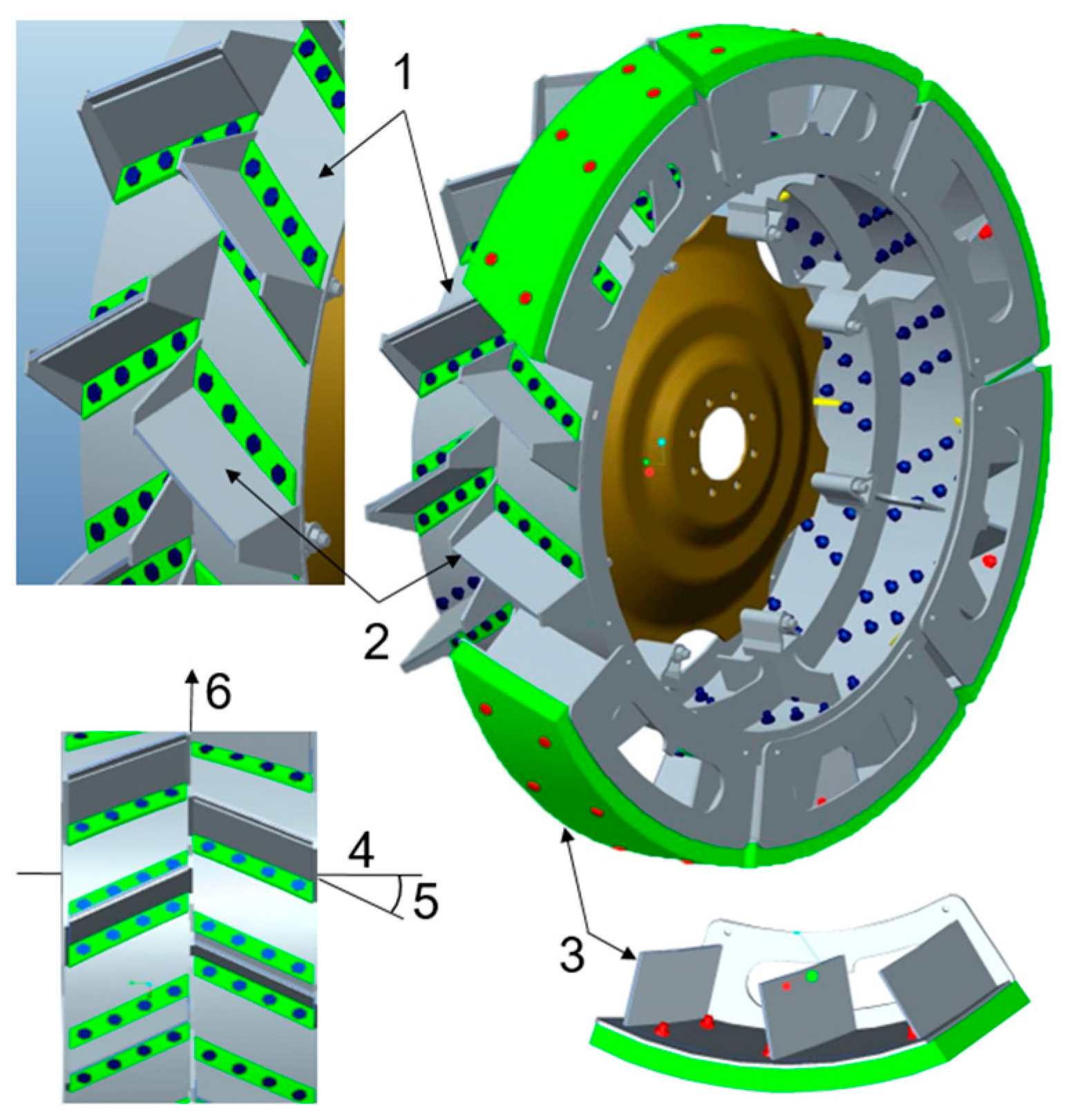
2.3.1. Wheel Structure

The whole wheel structure of the rigid lugged wheel consists of three main functional components. (1) Rim, including internal strengthening supports and mounting accessories. (2) Lugs that are arranged on the rim in herringbone arrangement at a 30° mounting angle with the axis of the wheel and lug height of 150 mm were set for optimum traction and driveability performance. (3) Road pad/rubber pad assemblies with internal supports and outer rubber pad that can be mounted to the wheel for on-road drive.
The main function and purpose of a rigid lugged wheel are field drive and adequate traction force provision for high-draught implements in diverse agricultural field conditions. Therefore, the road pad assemblies are only accessory items for minor road drives, while the rim and lugs are two major components for the functional requirements. The main design considerations were given to the two components, and some details of the designs are as follows:
The rim of the rigid lugged wheel is designed according to mounting provisions available for the tire wheel, as the same is used for rigid lugged wheel mounting, and according to available space and the drive mechanism. The width of the rigid lugged wheel rim was kept as wide as possible according to the drive criteria of the tractor and optimum working performance. Rim setting was adjusted to withstand all terrain/soil conditions and all working environments, such as dry and hard-untilled surfaces, soft loose tilled soil, and wet or saturated soil working conditions, and to avoid soil sticking and wheel blocking during wet soil field operations.
The main research object of this study was the lug of the rigid lugged wheel, so the design parameters of the lug are of much importance. On the lug, the working faceplate was the more specific object to design, arrange, and analyze for optimum wheel performance. The driving force of the lug is dependent on working surface parameters such as length and width, the mounting angle of the lug with the wheel axis, the angle of the lug’s working faceplate according to the reference axis, and its interaction with soil (soil penetration). Therefore, consideration was given to lug design, and analysis was performed for lug design and lug arrangements.

2.3.2. Design of Lug Working Faceplate

Figure 2a shows the fixed coordinate system “xyz”, where: the x-axis is the iron wheel axis, the y-axis points to the tractor’s forward direction, and the z-axis is vertically upward. In the “xoyozo” coordinate system, that is obtained by rotating “xyz” about 30 degrees in the positive direction (counter-clockwise) around the z-axis.
In this way, the z-axis remains the same, and the transformation relationship between the coordinate systems “xyz” and “xoyozo” is as follows:
  x = x o cos α y o sin α y = y o cos α + x o sin α z = z o                              
In the “ x o y o z o ” coordinate system, the small ellipse at the lug base of the iron wheel (as shown in Figure 2b) corresponds to the following equation:
x o 2 sin 2 α R 2 + z o 2 R 2 = 1
where: R = 1276/2 = 638 mm is the radius of the iron wheel rim; α = 30°; the small elliptic equation (2), now written as a parametric equation:
x o = R sin α .   sin θ y o = 0                 z o = R . cos θ
In Equation (3), θ is a small ellipse parameter, and the equation of a small ellipse in the xyz coordinate system is:
x y z = A R sin α . sin θ 0 R cos θ
By putting it in Equation (1), it results in:
x y z = A R tan α . sin θ R sin θ R cos θ
The range of x in the equation (according to Figure 2b) is 345 x 140 .

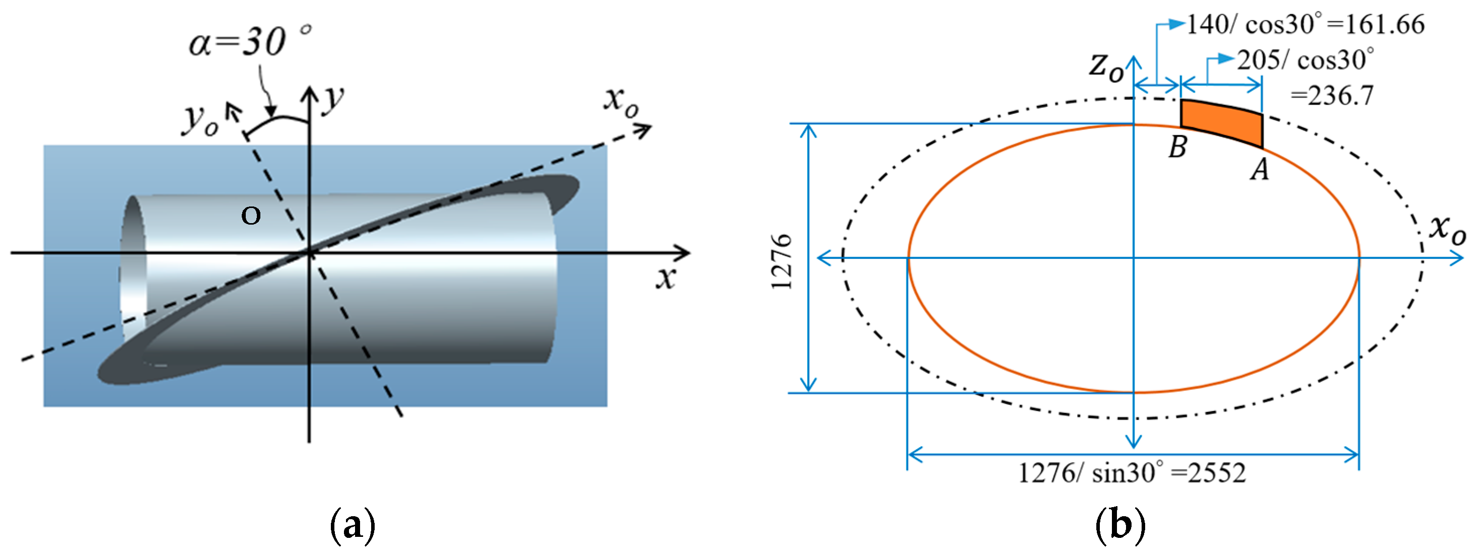
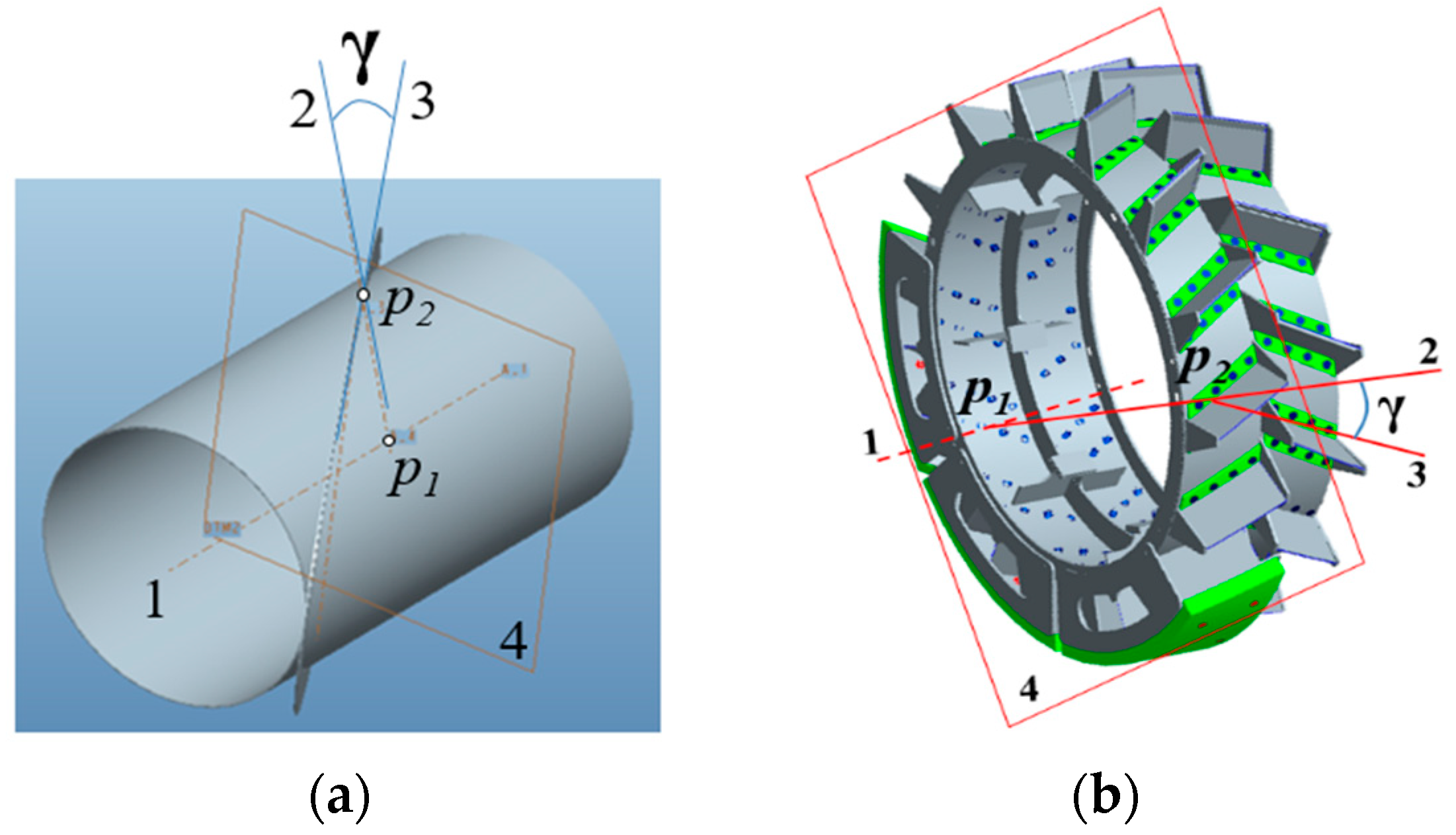
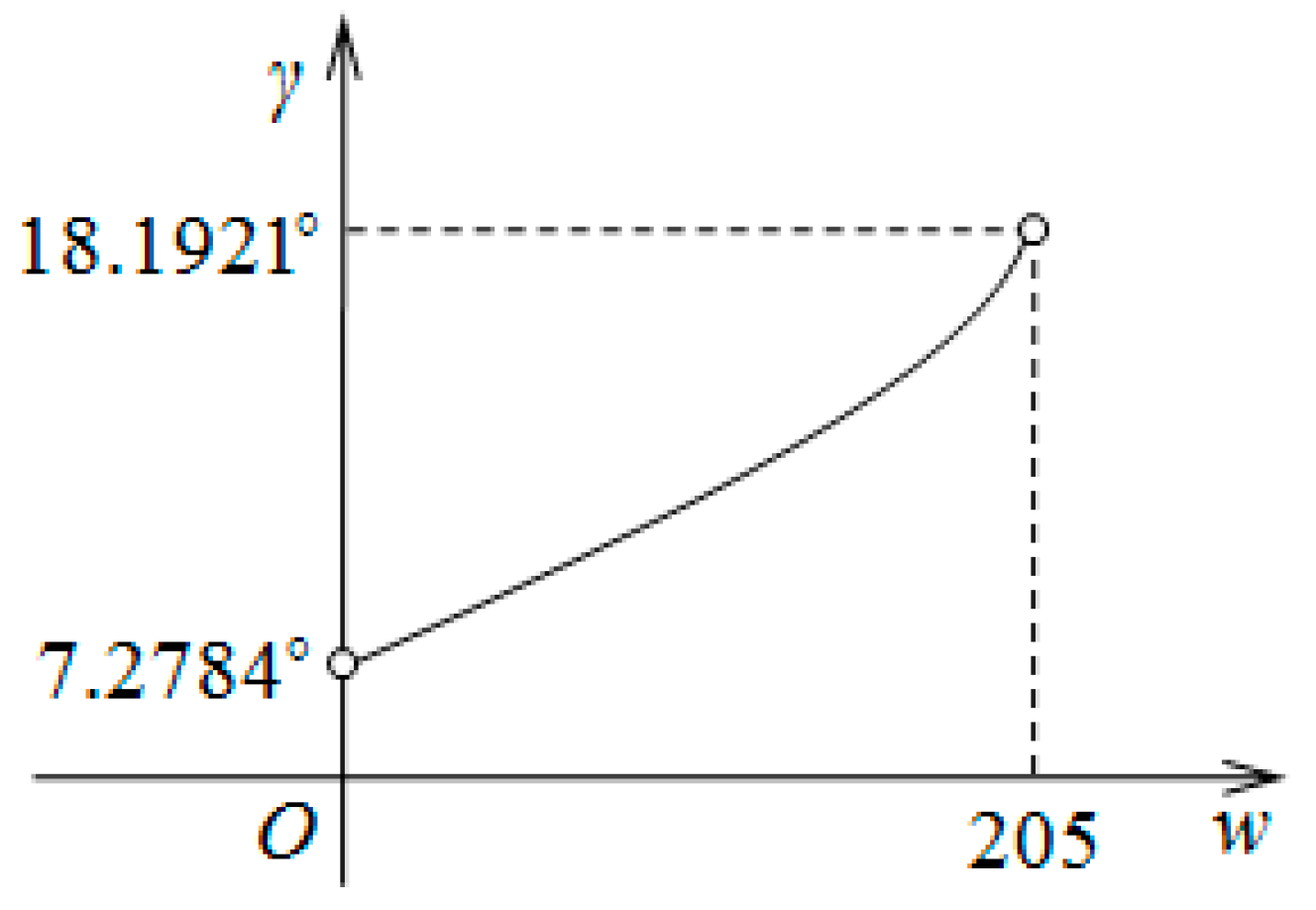
2.3.3. Mounting Angle of the Lug Working Faceplate

As shown in Figure 3a,b, line 1: iron wheel axis; plane 4: is a plane perpendicular to line 1 wheel axis; point p1: is the intersection of plane 4 and line 1 wheel axis; point p2: is the intersection of plane 4 and smaller elliptic curve; line 2: the intersection of point p1 and point p2. line 3: intersect line 2 at point p2 and go along the wheel lug surface and plane 4; angle gamma (γ): mounting angle of iron wheel lug faceplate; that is the angle between line 2 and line 3 at vertex point p2.
In Figure 3, the obliquely upward direction vector of line 2 obtained from Equation (4) is as follows:
n 2 = R sin θ .   j + R cos θ . k
In the coordinate system xyz, line 3 is parallel to the z-axis, so the angle between line 2 and line 3 is the angle between the vector and the z-axis.
cos θ = cos γ ,    
where: θ = γ.
That is, the installation angle of the lug is equal to the parameter theta (θ) in the small elliptic parametric equation.
From Equation (4):
x = R sin α   . sin θ     θ = γ = s i n 1 x tan α R
In the above equation, the value range of x is [140,345]; α = 30°; R = 638 mm;
The width of the lug along the axis of the iron wheel is 205 mm (see Figure 2b). The variable x in Equation (7) is replaced by the lug width parameter w (range: 0 to 205):
θ = γ = s i n 1 w + 140 tan α R
According to Equation (8), the relationship curve between the installation angle of the lug and the width “w” along the axis of the wheel can be drawn, as shown in Figure 4.
To verify the correctness of Equation (8), the values of the installation angle “γ” at different values of w are obtained by a ProE three-dimensional modeling test, and the results are compared with those calculated by Equation (8). The results are shown in Table 1. Comparisons between measured values of the three-dimensional model of installation angle gamma and calculated values of theoretical Equation (8) at different values of w.
Because of the ProE 5.0 version of the three-dimensional software, its measurement accuracy is four digits after the decimal point. From Table 1, we can see that Equation (8) for calculating the installation angle γ is correct.

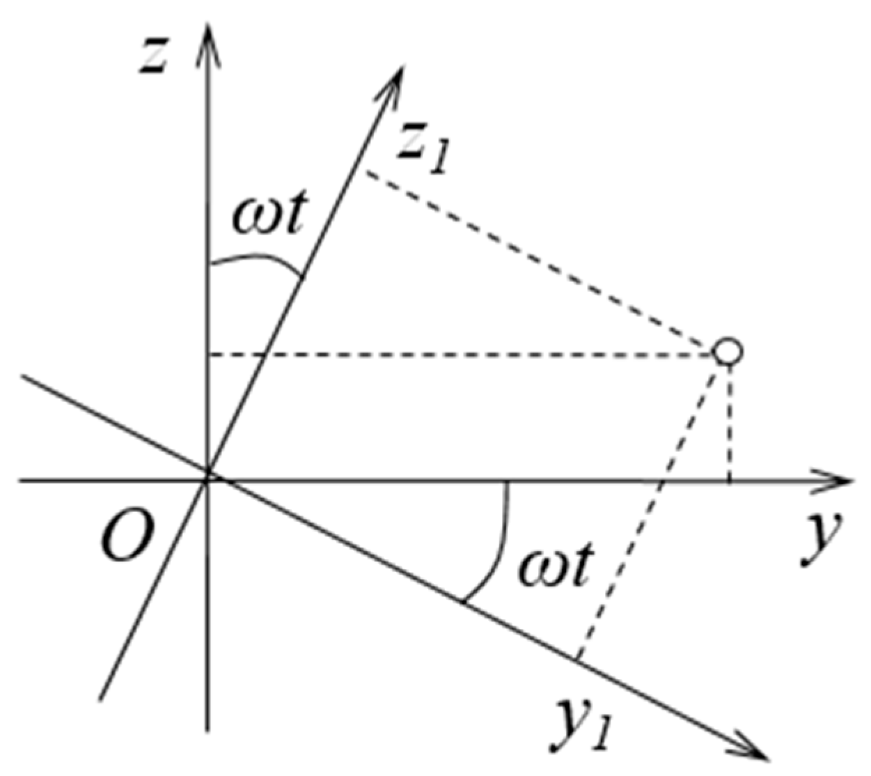
3. Kinematic Analysis

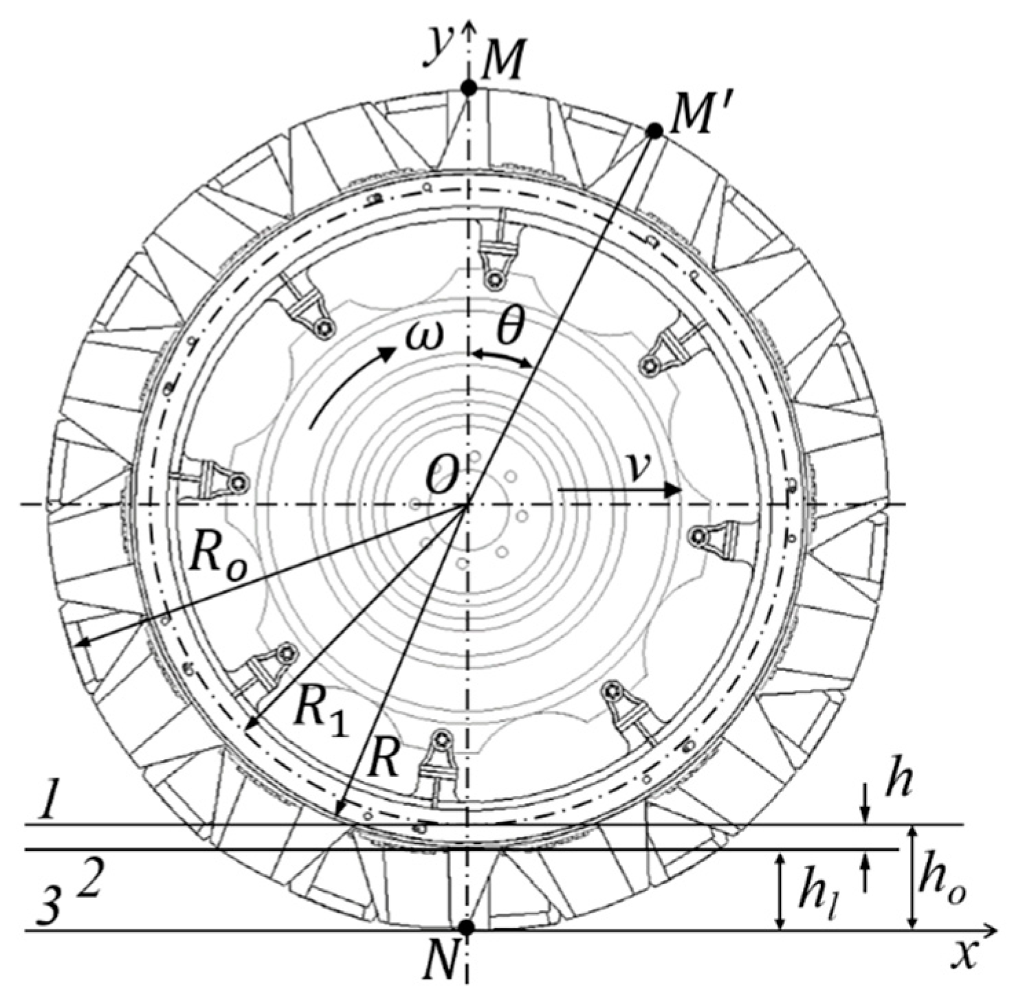
3.1. Driving Wheel Rotational and Translational Motion Relationship

It is assumed that when the tractor is driven on hard non-deformable or soft deformable terrain, the vehicle body maintains its movement in the horizontal plane. The vertical position is not affected by the rotation of the driving wheel, which is the rigid lugged wheel. Therefore, the driving wheel axis maintains a horizontal plane of movement. The radius R o represents the rolling radius of the wheel on hard un-deformable terrain; on soft, deformable terrain, when lugs penetrate the soil and the rim is not submerged, the rolling radius of the wheel is R , which is the radius of the rim. If the rim is submerged, R 1 represents the rolling radius of the wheel.
In Figure 5, the point “O” represents the wheel center or axle point of the rear axle of the tractor that moves along the horizontal direction with velocity “ v ” when the driving wheel rotates with an angular velocity “ ω ”. This is pure rotational movement along imaginary plane 1, which is the ground surface. A perpendicular line passes through the axle point O, and the point of intersection with plane 1 is the instantaneous axis of rotation.
To produce the driving force through wheel-terrain interaction to move the tractor on the soft, deformable soil, the wheel rotates under the action of applied torque and normal load on the wheel. In this process, some slippage happens between the wheel and the terrain due to the shearing and sliding of surface soil. Ideally, the driving wheel rotates without slipping or sliding.
Figure 5 shows that the actual rolling motion of the driving wheel is in accordance with plan 3. The velocity v t is the theoretical velocity of the point “O”, and “ R o ” is the maximum rolling radius, with “ ω ” as the angular velocity. Equation (9) can be used to calculate the theoretical velocity.
v t = R o . ω  
During the driving of a tractor for practical applications such as soil tillage, a certain amount of slip is always produced by the driving wheel, even without towed load conditions. Therefore, the actual velocity “ v ” of the tractor is less than the theoretical velocity “ v t ”. Equation (10) is used to calculate the actual velocity.
v = R 1 . ω
where, R 1 is the equivalent radius or actual rolling radius of the wheel in operational conditions. The loss of velocity caused by the slipping or shearing of the driving wheel over the terrain surface during the driving process is called travel reduction T r and can be calculated by the following equation:
T r = v t v v t = 1 v v t
The rolling radius of the driving wheel varies with field operational conditions, terrain properties, wheel structural parameters, applied normal and drawbar loads, and several other factors. Therefore, in practice, it is inconvenient to use the actual travel reduction for theoretical computations and analysis. Therefore, the maximum radius R o of the rigid lugged wheel is used for the calculation of travel reduction by using Equation (12).
T r = 1 R 1 R o
The rolling radius of the tractor wheel changes with the applied drawbar or traction load, which can be determined during the field-driving test. If the tractor operated at wheel rpm n under a certain applied load and traveled a certain distance s, the rotating radius of the wheel could be calculated by the following equation:
R 1 = s 2 π n
The tractor wheel radius, R 1 may vary according to the terrain and operational conditions; it is used for kinematic and dynamic analysis and determination and calculation of tractor traction performance parameters in field operations with the applied drawbar.

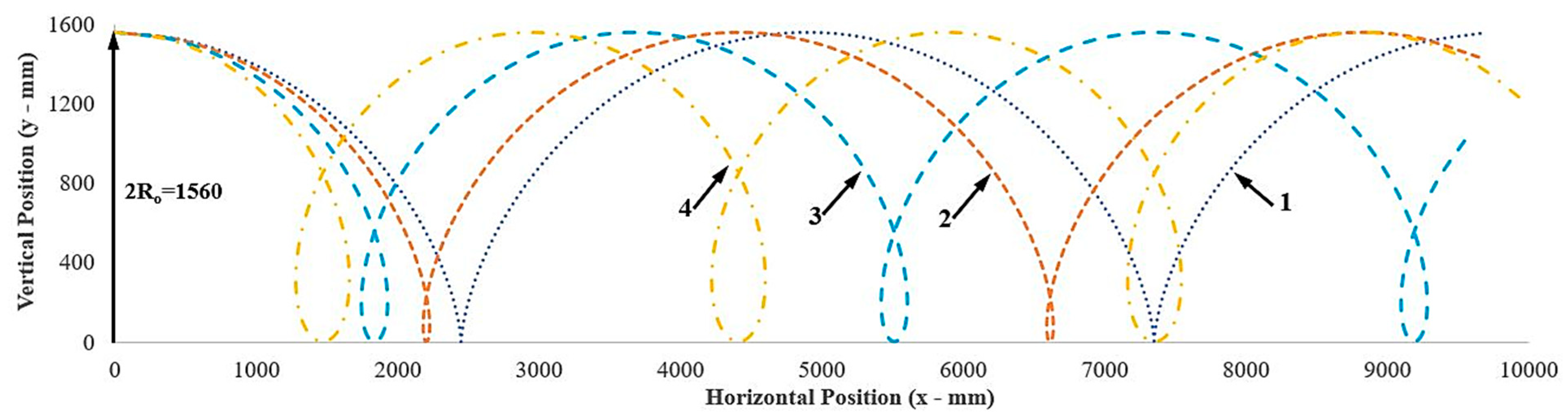
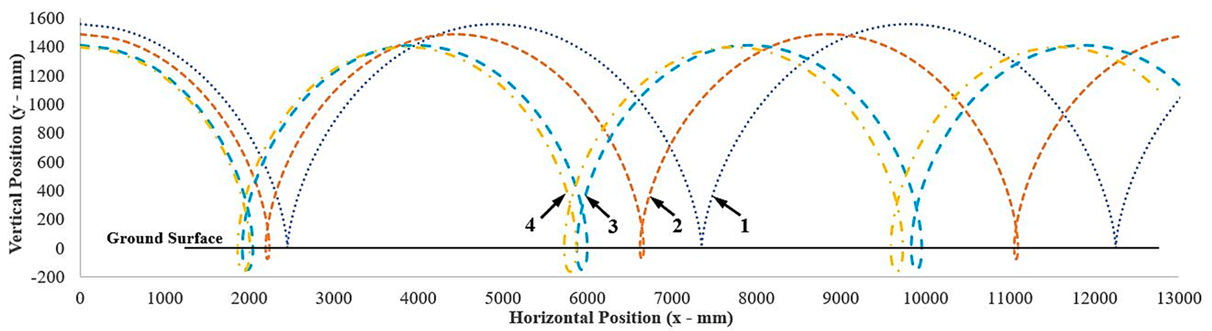
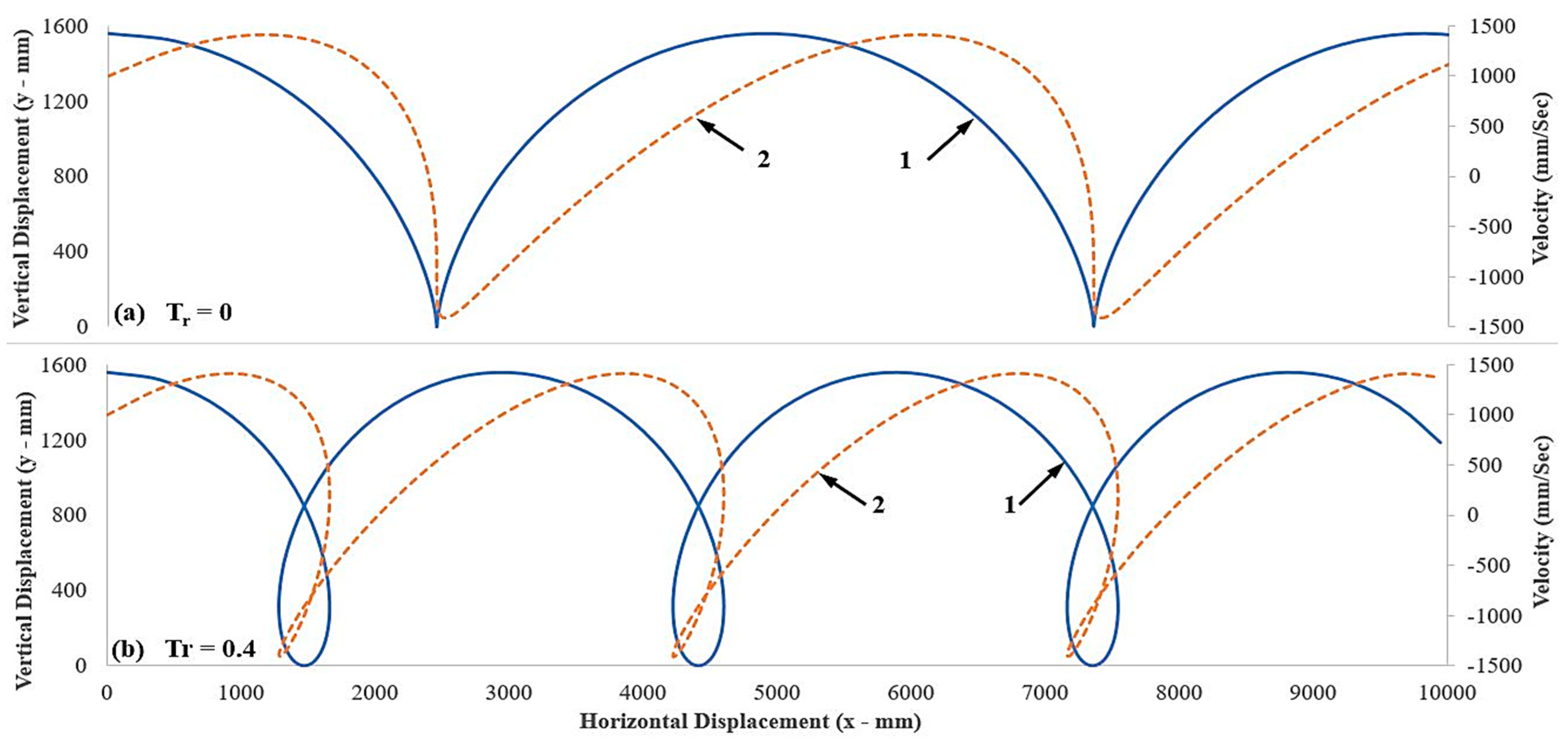
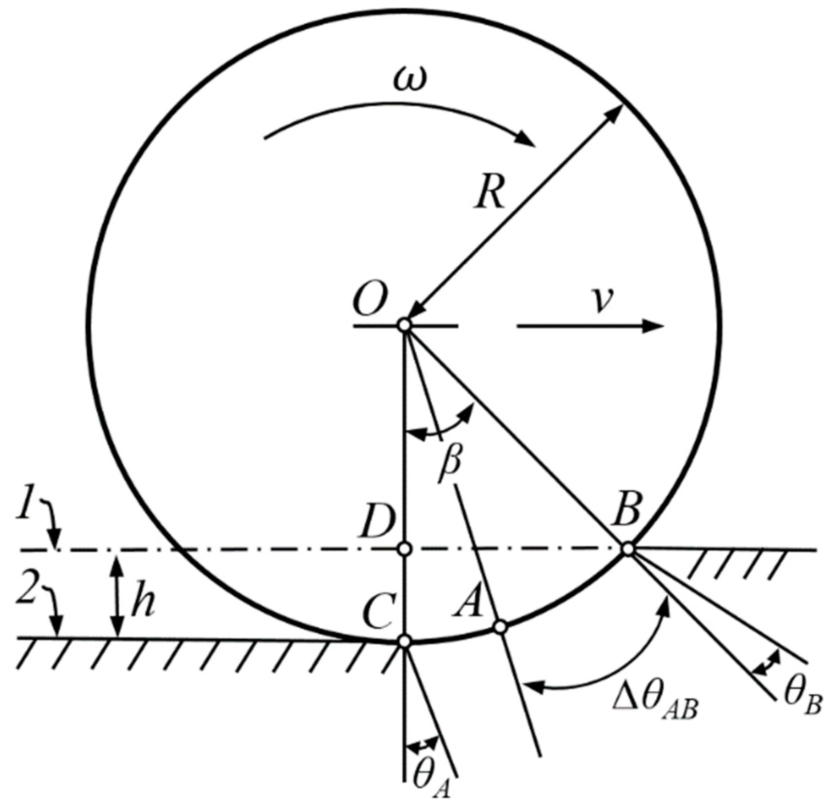
3.2. Motion Trajectory of the Lug Tip of the Rigid Lugged Wheel
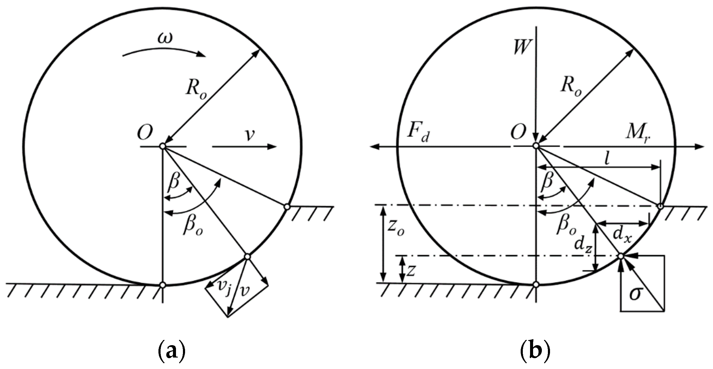
While the driving wheel “rigid lugged wheel” rotates on the loose terrain/ field soil surface, the lugs of the wheel continuously pass through the soil. This process forms the cut marks in the soil that reflect the interaction between the wheel and the terrain soil. Therefore, it is important to analyze the wheel-soil interaction relative to the motion of the wheel to determine the stresses of the wheel lug on soil and the soil cutting and shearing process. The theoretical shape and size of the lug cut hole are determined by the motion trajectory, and they change with the structural parameters of the wheel lug, slip rate, i.e., travel reduction of the driving wheel, and height of lug penetration/wheel submergence.
When the rigid lugged wheel is driven on a flat, non-deformable surface, the terrain surface contact points are located on the tips of the lugs, which are the highest points on the wheel’s outer radius along the vertical axis. Therefore, kinematic analysis of the rigid lugged wheel is equivalent to finding the rotational and translational conditions of the contact points. A diagram representing the rotational conditions of the rigid lugged wheel with axes and plans of motion is shown in Figure 5, where point O represents the center of the wheel or wheel rotation axis that is at a height from the plan of motion (line 3) equivalent to the radius R o . A point M located on the tip of the lug in rest condition at time t = 0 has coordinates X M = 0 , which means the horizontal displacement is 0, and Y M = 2 R , which is the height of point M from the ground surface equal to the wheel diameter.
Assuming the wheel begins to rotate and moves with a uniform angular velocity ω and a linear velocity v . After a time t , the point M turns into M . By subtending an angle θ (Figure 5), the coordinates of the point M with respect to the ground-surface contact point reference frame can be determined by the following equations:
X M = R o   θ + R o sin θ
Y M = R o + R o cos θ      
The above equations are for ideal motion without slipping on a hard plain surface. However, in real conditions, in which wheels slip and slide on the terrain surface, the slip factor should be included, and the maximum radius, R o , should be replaced with the equivalent radius,   R 1 , that is defined in Equation (13). Therefore, the equations to determine the position of the point are as follows when θ = ω t :
X M = 1 T r   R 1   ω t + R 1 sin ω t
Y M = R 1 + R 1 cos ω t      
From the above equations, it is found that the motion trajectory of point M is associated with the rolling radius of the rigid lugged wheel and the wheel travel reduction rate. The motion trails of point M with different travel reduction rates are shown in Figure 6, and with different lug penetration or wheel submergence in Figure 7. The vertical axis (y-axis) represents the vertical position of the point, and the horizontal axis (x-axis) represents the horizontal position of the point at any instant of time while the wheel is rolling. The curves 1, 2, 3, and 4 in Figure 6 represent the trajectories of point M with a travel reduction rate of 0.0, 0.1, 0.25, and 0.4, respectively. Curve 1 is the trajectory of a point with ideal motion without slip, which means no travel reduction, and this pattern of motion is called cycloidal motion. Curves 2, 3, and 4 show the reduction in horizontal distance traveled per rotation of the wheel to calculate the travel reduction rate. As the travel reduction rate increases due to slipping and shearing between the surfaces, it produces more soil breakage and damage and reduces the distance traveled. Curves 1, 2, 3, and 4 in Figure 7 represent the trajectories of point M with lug penetration and wheel submergence of 0, 75, 150, and 165 mm, respectively. The effect of lug penetration and wheel submergence on rolling motion and horizontal distance traveled is obvious.
The instantaneous velocity v M   of point M at any instant of the time can be determined by the following equation for the center of the wheel reference frame when the wheel is rotating with uniform angular velocity ω and translating with a uniform linear velocity v :
v M = R 1   ω sin ω t + R 1   ω   c o s ω t
When the rigid lugged wheel undergoes pure rotation at a certain velocity, the relationship between the vertical displacement and velocity of the edge points of the wheel lugs is shown in Figure 8a. The vertical axes (y-axis) denote the vertical displacement and velocity of the point. The horizontal axis (x-axis) denotes the horizontal displacement. Curves 1 and 2 represent the vertical displacement and velocity of the point M respectively. When the rigid lugged wheel goes through pure rotation at a slip rate of 0.4 on the soft deformable terrain surface, the relationship between the vertical displacement and velocity of the edge points of the wheel lugs is shown in Figure 8b. Curves 1 and 2 represent the vertical displacement and velocity, respectively.
A comparative analysis of Figure 8a,b indicates that when the drive wheel slips, the displacement and velocity of the wheel lug tips (contact points) are repeated in the space. Thus, the vertical displacement and velocity of the wheel occur at lug tips or edge points, and the motion condition that is produced is more complex than pure rotation.
The impacts of the soil on the wheel during the wheel-soil interaction process produce power losses. The motion or rolling resistance is produced by the wheel penetration/sinkage and the soil reaction force, which is generated as the wheel lug penetrates and breaks/excavates the soil. The wheel lug impacting the soil backward also produces power losses, but it is necessary to obtain a wheel thrust or drive force from the soil.

4. Dynamic Analysis

4.1. Determination of the Lugged Wheel Driving Force

4.1.1. The Normal Vector of the Lug Working Surface

In the xoyozo coordinate system, the normal vector of the working surface of the lug is ( n o = j ), by combining Equation (1), the normal vector of the lug working surface in the xyz coordinate system is:
n = A .   n o   ,   where :   n x n y n z = sin α cos α 0
In the process of cultivation or tillage, the tractor’s forward speed is v m , along the positive direction of the y-axis. The angular speed of the iron wheel is ω, along the negative direction of the x-axis. Then, there is a rotation and translation transformation relationship between the coordinate system x1y1z1 fixed on the iron wheel at the time ‘t’ and the fixed coordinate system xyz at the beginning, and the rotation transformation relationship is shown in Figure 9.
From Figure 9, following equation is derived:
x 1 = x                                 y 1 = y cos ω t z sin ω t   z 1 = z cos ω t + y sin ω t
Assume:
x 1 y 1 z 1 = B   x y z   x y z = B 1 x 1 y 1 z 1 ,
where
B = 1 0 0 0 cos ω t sin ω t 0 sin ω t   cos ω t
and
  B 1 = 1 0 0 0 cos ω t sin ω t 0 sin ω t cos ω t
Considering the rotation and translation relationship between the coordinate systems x1y1z1 and xyz, there is:
x y z = B   x 1 y 1 z 1 + 0 v m t 0
By adding Equation (19) to Equation (20), the expression of the normal direction vector of the lug working surface in the fixed coordinate system xyz is obtained as follows:
n t = n t x n t y n t z = B 1   .   n =   sin α                   cos α   . cos ω t cos α   .   sin ω t                                      

4.1.2. Driving Force Analysis of the Lug

Most of the upland farming areas in China cultivated two crops a year, so farmers tilled the soil twice a year with rotary or vertical tillage implements. Considering the physical characteristics of farmland soil, we can characterize it as an isotropic and completely plastic material. This study assumes that the depth of surface soil compacted by the iron wheel due to submergence of the iron wheel rim of radius R = 638 mm during cultivation is h = 15 mm, as shown in Figure 10. According to this figure:
R   1 cos β = h   a n d   β = cos 1 R h R    
By the above equation, the value of β is:
β = 12.4488 ° = 0.217273   r a d .
As the width of the iron wheel B = 440 mm, the wheel soil contact area of the iron wheel rim is:
S o = R × β × B ,
It results in: So = 60992.75144 mm2.
Equation (4) was used to determine the corresponding position of two points A and B in Figure 2b, where x A = 345 and x B = 140 were on the lug in the fixed coordinate system xyz:
x A y A z A = R tan α . sin θ A R sin θ A R cos θ A   and   x B y B z B = R tan α . sin θ B R sin θ B             R cos θ B           .              
By taking xA = 345 and xB = 140 into the above equation, it results in θA = 18.19° and θB = 7.28°, respectively, and by putting them in Equation (21), the trajectory equations of points A and B are obtained in return as:
x A t y A t z A t = B 1 x A y A z A + 0 v m t 0 = 345 R sin θ A cos ω t + R cos θ A sin ω t + v m t R sin θ A sin ω t + R cos θ A cos ω t
That resulted in the following equation:
x A t y A t z A t = 345                               R sin ( ω t + θ A ) + v m t R cos ( ω t + θ A )          
and
x B t y B t z B t = B 1 x B y B z B + 0 v m t 0 = 140                                                                         R   sin θ B   cos ω t + R   cos θ B   sin ω t + v m t R   sin θ B   sin ω t + R   cos θ B   cos ω t        
x B t y B t z B t = 140                                 R sin θ B + ω t + v m t R cos θ B + ω t          
Based on ProE three-dimensional software modeling and measurement, the area of the lug working surface shown in Figure 2b, is S = 34,343.2 mm2. The force or soil thrust on the lug’s working surface is related to the reaction force of the lug on the soil. Regardless of the friction force between the soil and the lug surface, it is assumed that the normal pressure of the soil on the driving or working surface of the lug is p l , the unit of which is N·m−2. By using Equation (22), the positive pressure of soil, i.e., soil thrust, on the working surface of the lug is as follows:
F = n t x n t y n t z . S . p l = S . p l . sin α           S . p l . cos α cos ω t S . p l . cos α sin ω t
In the equation:
S = area of lug working surface (34,343.2 mm2) it varies with the height of penetration of the lug, p l to be determined represents the compressive or normal stress of soil on the lug working surface, ω =1.28 rad s−1, and 2.37 s ≥ t ≥ 2.18 s.
Equation (27) shows that the axial component of the soil thrust acting on the lug, i.e., the x-axis component, is a constant, i.e.,
F x = S . p l . sin α = 0.5 S p l  
Therefore, the axial component accounts for 50% of the total force.
The component of soil thrust acting on the lug working surface that helps to move the whole machine in the forward direction is the y-axis component, which is to say, the driving force provided by the interaction of the wheel lug and soil is:
F y = S   .   p l   .     cos α   . cos ω t F y = 0.9413   ~   0.9950 .   S .   p l .   cos α F y = 0.8152   ~   0.8617 S .   p l                                    
It can be seen that the lug’s driving force is proportional to the angle α the smaller the angle, the greater the driving force. In addition, the driving force of the lug is related to the relative alignment of the working surface in the soil. In the beginning, the driving force is the smallest when the lug starts to penetrate and gradually increases until it is completely submerged in the soil. The fluctuation range of the driving force is 81.52% to 86.17%.
The vertical component of soil thrust acting on the lug is as follows:
F z = S   .   p l   .     cos α   . sin ω t F z = 0.3375   ~   0.1001 .   S .   p l .   cos α F z = 0.2923   ~   0.0867 .   S .   p l                
It can be seen that the vertical force decreases from 29.23% to 8.67%. The smaller vertical force helps to reduce the compaction effect of the whole machine on the soil [19,20].

4.1.3. Soil Thrust-Driving Force Relationship Analysis of Lugged Wheel

Predicting the normal pressure p of soil applied to the wheel contact surface or p l = p applied to the lug working surface is critical for analyzing the tractor drive wheel’s traction performance. The principles used to predict the soil mechanical behavior and response under wheel loading are called the pressure-sinkage relationship and shear failure criteria. The pressure-sinkage relationship suggested by scientists who worked on soil mechanics is presented in Equation (30) [21].
p = k z n  
This pressure sinkage relationship states that the average pressure applied to a plate on a uniform terrain is dependent on an exponential function of sinkage ‘z’, in which the exponent ‘n’ represents a soil property reliant on the size of the wheel and ‘k’ is the proportionality constant. A more explanatory and descriptive form of the pressure sinkage relationship of vehicle wheels is presented in Equation (31), which is a more widely relied-upon expression and is used in the practice of terramechanics and vehicle traction mechanics [21].
p = k 1 b + k 2 z n  
The proportionality constant ‘k’ has been revised to justify the dimensions of the contact area. The letter b represents the wheel width, and k1 and k2 remain parameters of soil sinkage. The soil parameters n, k1, and k2 are empirical and have no intrinsic physical meaning. The parameters can be determined by pressure-sinkage data from field experiments. Although the pressure sinkage relationship is a semi-empirical expression, it is most important in terramechanics and tractor traction mechanics as the shear strength of the soil is mainly related to normal load (ground pressure). Additionally, the soil thrust developed under the drive wheel or wheel drive force and motion resistance is relative to sinkage (i.e., the relationship between pressure and sinkage).
The shear stress-displacement relationship, or share failure expression for maximum share stress and applied normal pressure, can be expressed by the Mohr-Coulomb equation that adequately describes the relation in many cases [17].
τ m a x = c + p   t a n ϕ  
To describe the shared stress-displacement relationship for a deformable terrain, an expression was suggested by [22], in which the researcher [23] proposed a modification for loose plastic soil that is presented in the following equation and widely adopted in practice.
τ τ m a x = 1 e j K
Therefore, Equation (32) has the following form:
τ = c + p   t a n ϕ 1 e j K                        
In the above expression, τ is the shear stress, j is the soil shearing displacement, K is the shear modulus, which can be determined by fitting the shear stress-shear displacement equation [23] to each data set, c is the soil cohesion, and ϕ is internal friction angle, which can be determined by the Mohr-Coulomb failure criteria.
The share displacement that is developed along the contact patch of the rigid wheel can be determined by analysis of the slip velocity v j on the wheel-terrain interface, as shown in Figure 11a [17,24,25]. The tangential component of the absolute velocity v of a certain point on the circumference of the wheel relative to the terrain is described as slip velocity v j [17]. The magnitude of the slip velocity v j of a point on the rigid wheel circumference defined by the angle β can, therefore, be expressed as below [24].
v j = r ω 1 1 T r cos β
The parameter j, which is the shared displacement of a point along the contact surface for rigid wheels and loose soil, can be determined by the following equation:
j = 0 t v j   d t = 0 β o r ω 1 1 T r cos β d β ω j = r β o β 1 T r sin β o sin β
According to soil shear theory and wheel-terrain interaction, the rigid lugged wheel has two main soil reaction forces along the y-axis: (1) F s due to the shear stress τ between the wheel bottom surface and soil surface, and (2) F l due to the normal terrain pressure p on the lug working surface.
The thrust-slip relationship for a rigid wheel, Equation (37), can be determined by using the shear stress-shear displacement relationship, Equation (34), by considering uniformly distributed normal pressure and the flat wheel-terrain contact patch of contact length l and contact area A [17].
F = A c + p tan ϕ 1 K T r   l 1 e T r   l / K            
where c, ϕ, and K are the cohesion, angle of shearing resistance or internal friction, and shear deformation parameters of the terrain material, “the surface soil”, respectively. T r is the travel reduction due to the wheel slip, and p is the normal pressure on the wheel-terrain contact surface that is equal to the normal load of the wheel on the contact surface.
As the front contact angle of the rigid lugged wheel is determined (i.e., 0 β o ) (Figure 11) [17], the rigid lugged wheel thrust force or drive force, F s , can be determined by integrating the stresses over the wheel-terrain contact surface.
F = F s = b R o 0 β o τ β cos β   d β = b R o   0 β o c + p   t a n ϕ 1 e j / K   c o s   β   d β
F = F s = b R o 0 β o c + K 1 b + K 2 R o n cos β cos β o n t a n ϕ 1 e R o β o β 1 T r sin β o sin β / K c o s β d β
From the above equation, it is found that the driving force of a rigid lugged wheel is related directly to wheel width, radius, and sinkage and inversely to travel reduction rate.
When the tractor is operating on soft terrain and the majority of the rigid wheel’s lugs are submerged in the terrain, the terrain material/soil fills the spaces between the lugs. In this case, the rigid lugged wheel acts like a smooth rigid wheel (Figure 11), so Equation (38), can be used for the thrust/drive force analysis of a rigid lugged wheel. However, over medium to hard terrain, the entire wheel load may be supported on the tips or faces of lugs, and there is minimum or no contact of the carcass (rim surface) with the terrain. In this case, the thrust-sinkage analysis, already done for the single lug, Equation (28), can be used by integrating the stresses over the whole contact area of lugs or the number of lugs by considering ( ω t = β ) as follows:
F = F l = S cos α 0 β o p l . cos β d β = S cos α 0 β o K 1 b + K 2 R o n cos β cos β o n cos β d β
The net driving force,   F d , produced by wheel-terrain interaction can be found by:
F d = F M r
Rolling resistance or motion resistance M r to the wheel of a moving tractor on deformable terrain could be produced due to the penetration of lugs and sinkage of the wheel. The power consumed in the motion resistance of the tire wheel is equal to the work conducted on soil compaction and rut formation, but in the case of high lugs rigid wheel, work is expended on the breaking and loosening of soil by the penetration of sharp-edged lugs.
M r = b 0 β o σ   R   S i n β   d β
The radial pressure σ applied on the wheel due to wheel-terrain interaction (Figure 11b) is equal to the normal pressure p below a sinkage plate at the same sinkage depth z in a pressure sinkage test; therefore, the following expression is developed.
σ R . s i n β   d β = p   d z
By combining the pressure-sinkage relationship with the above equation and including the effect of travel reduction rate, the motion resistance of a rigid wheel can be determined as follows:
M r = b 1 T r 0 z o k 1 b + k 2 z o n   d z = b 1 T r k 1 b + k 2 R o cos β cos β o n + 1 n + 1
where z o represents the wheel’s maximum sinkage, as shown in Figure 11b. The above analysis shows that the motion resistance of a rigid lugged wheel depends on the wheel width, wheel radius, and sinkage depth; a higher travel reduction rate also causes higher motion resistance.
From the dynamic analysis of the rigid lugged wheel, it is found that the forces on the wheel include shear and normal stresses on the wheel rim and normal pressure on the wheel lug working surface. The normal pressure on the lug working surface results in a higher driving force from the rigid lugged wheel that is independent of the wheel axle’s normal load. The motion resistance of a rigid lugged wheel could be higher due to the penetration of lugs into the soil, but this will help to break and loosen the soil and get compensated by the lower soil tillage draft. In this way, the rigid lugged wheel will help to consume tractor power efficiently and avoid soil compaction in soil tillage operations.

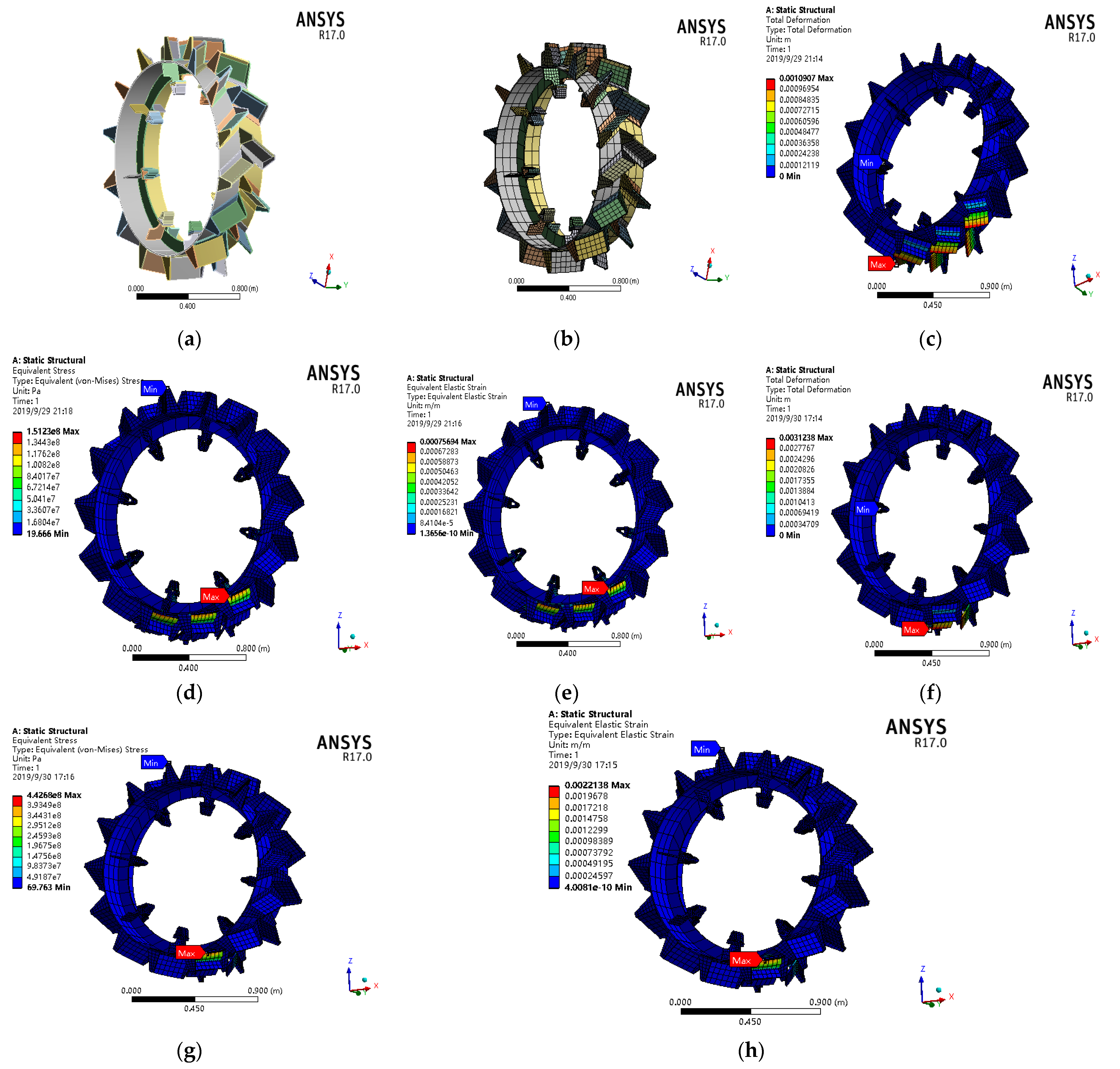
5. Model Evaluation (FEM Analysis) for Structural Stability and Optimization

The designed model of the rigid lugged wheel was analyzed in the ANSYS workbench platform for the structural optimization of a new wheel. The behavior of the structural components under applied forces on the designed model was analyzed on assessing stresses, strains, and deformations resulting from the analysis of applied loads. The purpose of this simulation analysis was to check the material suitability and design parameters to select the best-fit material and optimum parameters, e.g., the thickness of the steel sheet used for the wheel structure with the minimum wheel structure weight.

5.1. Material Properties (Engineering Data)

The material was selected based on design criteria, working conditions, and operational requirements. It was a Manganese Iron alloy called high Carbon Manganese steel (Steel No. 15 Mn) sheets that contain Carbon (0.12–0.18), Silicon (0.17–0.37), and Manganese (0.70–1.00) percent as chemical mass fractions. The engineering properties data of the material are as follows: the density of 15Mn steel is 7.8 × 10³ kg m−3, the modulus of elasticity is 200–220 G Pa, and the Poisson’s ratio is 0.25–0.30. In the field, tractor wheels are constantly stressed and, in extreme cases, face high-intensity impact loads. The material used for the fabrication of the newly designed modern type rigid lugged wheel was chosen considering all possible loading conditions so that it can safely withstand applied stresses and all types of loads.

5.2. Static Structural Analysis

The structure of the rigid lugged wheel under static loads was analyzed for structural stability and optimization using ANSYS Workbench mechanical simulation software. ProE’s (Creo Elements) 2D and 3D engineering design platform was used to generate 3D wheel model geometry, and the entire wheel structure assembly was saved in “igs” file format, which is compatible with and importable into ANSYS Workbench. In ANSYS R17 Workbench, the static structural project solver was used for analysis, engineering data was modified according to test specifications and analysis requirements, and the ‘.igs’ geometry file was imported into the project schematic. After making some corrections and modifications, the final structure model was prepared, and the mesh was applied in Figure 12a,b. The meshing, loads, supports, and displacement setup were defined, and resulting behavior parameters, e.g., stress-strain and deformations were selected. The project was analyzed by the problem solver option in the design modeler of ANSYS. Results were generated in graphical form (color schematic), as presented in Figure 12c–h which explained the effect of applied loads on the wheel body.
The reaction force, or soil thrust, developed on the wheel against the normal weight of the tractor and applied torque that acted on the lug working surface as the lugs of the wheel were in direct contact with the soil. The normal component of reaction forces to the lug-working surface provides the drive and traction force to the tractor. Therefore, the total force applied to the lugs would be equal to the maximum drawbar force of the tractor. To avoid the failure risk of the wheel structure in adverse field conditions, 20% of the total force was included as a safety factor.
In terms of the contact surface with the wheel, two different field conditions were considered. The first one was soft, easily penetrable soil where the whole lug can penetrate easily; in this case, a total of six lugs were considered to be in contact with the soil. In another case, the soil was hard enough that it allowed very little penetration, and only two lugs were in contact with the soil surface. The total force was divided accordingly in both cases; when force was divided among six lugs, there was less force per lug, so the stresses and deformations were less (Figure 12c–e) compared to another case where total force was applied only on two lugs, where stresses and deformations were higher (Figure 12f–h).
In both cases, the overall effects of loads and resulting stresses and deformations were very low and there was no situation was observed that affect the structural stability. Therefore, it is recommendable to suggest a reduced thickness of the steel sheet that might help to reduce the weight of the wheel, and ultimately, the total weight of the tractor helps to get optimum traction with minimum damage to the soil and the environment.

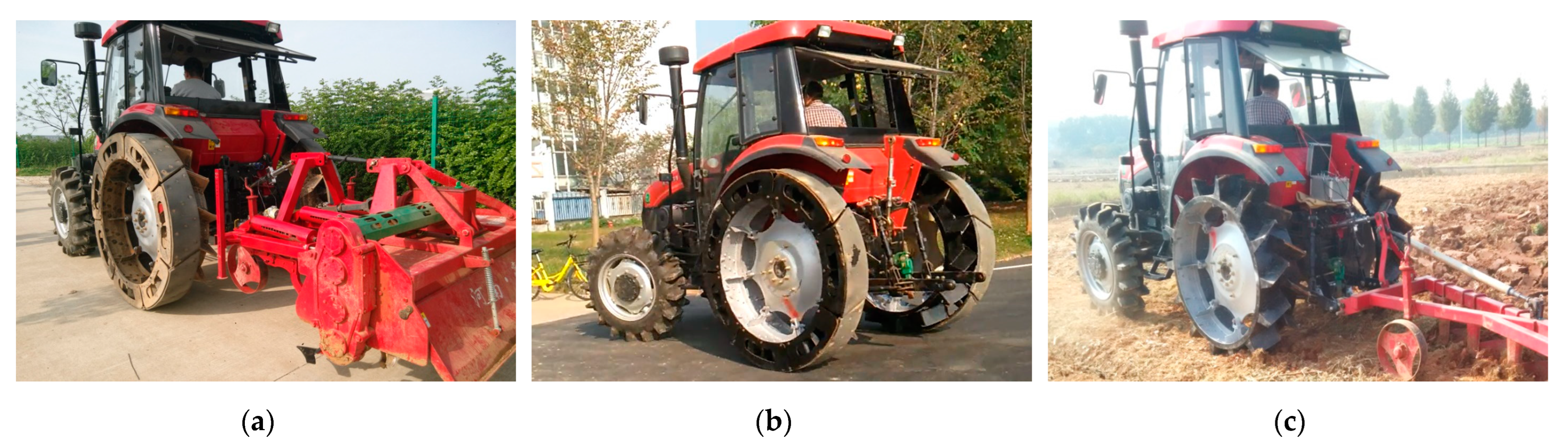
6. Wheel Prototype Development and Driving Tests

The designed rigid lugged wheel model was converted to a prototype after the structure stability analysis in the ANSYS workbench and verification of the designed parameters. Two rigid lugged wheel full-body structures were fabricated and developed according to the size and operational requirements of the specified tractor for this study. At a local industrial manufacturing factory, wheels were developed using a specific material (15Mn steel).
On-road drive and field tests were carried out to verify the design parameters, theoretical analysis, and traction performance (Figure 13), which represented the significant improvement in the wheeled tractor’s traction performance with rigid lugged wheels as drive wheels compared to conventional tire wheels. Traction and wheel-soil interaction performance of a rigid lugged wheel is already reported [2,4], and further studies and analyses are under process to verify the effectiveness of the rigid lugged wheel for off-road drive operations of the conventional wheeled tractor.

7. Conclusions

Traction demand from conventional agricultural wheeled tractors has increased in recent years for cultivation operations according to the requirement of intensive traction, improved trafficability, and drivability without increasing machine weight to avoid soil compaction and excessive energy consumption. A new design of a high lug rigid wheel is developed and tested as a traction device. The main component of the research object is the design of the lug working faceplate. The working principle of the rigid lugged wheel is theoretically confirmed by kinematic and dynamic analysis. The relationships and analysis are elucidated for wheel design parameters, terrain soil characteristics, rolling motion, and drive force generation behavior. A computer simulation of the designed model by the finite element method is presented that verifies the structure’s stability and provides a reference for optimization. The complete wheel structure is developed and tested on field conditions while the theoretical analysis/modeling and design parameters optimization are in process. The results of theoretical analysis and field tests are consistent, indicating that the rigid lugged wheel is well suited to soft deformable terrain, with improved traction and drivability. Theoretical analysis is performed for the newly designed rigid lugged wheel that provides in-depth theoretical modeling to assess and confirm its working principles. Insertion pressure, rather than shearing pressure, generates driving power in a rigid lugged wheel with a sharp edge and flat contact surface. In this way, it can produce higher traction, give A pre-tillage effect to the top soil, and reduces the tillage draught requirement. As confirmed by theoretical analysis, the component of thrust along the direction of driving ranged from 81.52% to 86.17%, which is actually the driving force and relates to lug faceplate alignment and lug penetration depth. Moreover, the vertical component of thrust reported was less than 30% and decreases further to less than 9% as the wheel displaces in the soil, which will avoid soil compaction under the wheel. To test lugged wheels’ field performance and conduct a comparative analysis with tire wheels, traction, and wheel-soil interaction performance are already been reported [2,4], which provide the validation base for these theoretical results. Further research on the rigid lugged wheel is required to improve the wheel structure parameters and adaptability in various adverse field conditions. The results of this study could provide a trusted technical reference for the future design and construction of off-road agricultural vehicles, agricultural tractors, and particularly traction devices/drive wheels for field operations.

8. Patents

High-power tractor drive wheel. Zhang Jumin, Xia Junfang, Zhou Yong, and Hafiz Md-Tahir. Huazhong Agricultural University. Patent No. ZL 2015 10922181.8. (2019). State Intellectual Property Administration Office of China, PR China.

Author Contributions

Conceptualization, H.M.-T. and J.Z.; methodology, H.M.-T.; software, H.M.-T. and J.Z.; validation, H.M.-T. and J.Z.; formal analysis, H.M.-T., M.S. and F.A.; investigation, H.M.-T.; resources, J.X., J.Z., Y.Z. and J.D.; data curation, H.M.-T.; writing—original draft preparation, H.M.-T.; writing—review and editing, H.M.-T., A.U. and Z.H.; visualization, H.M.-T., J.Z. and J.X.; supervision, J.X., J.Z. and Y.Z.; project administration, J.X., J.Z., Y.Z. and J.D.; funding acquisition, J.X. and J.Z. All authors have read and agreed to the published version of the manuscript.

Funding

Financially supported by: 1. National key technology research and development projects, National Natural Science Foundation of P.R. China, (Grant No. 32271994), entitled “Study on mechanism of detachment and consumption reduction in the soil-straw-machine interface for rice straw returning to soil in up-land paddy rotation farming”. 2. Ministry of Science and Technology of P. R. China, (Grant No. 2017YFD0301300) entitled “Key technology research on intelligent production of diversified cereal crops in double cropping system”.

Institutional Review Board Statement

Not applicable.

Data Availability Statement

The data presented in this study are available on request from the corresponding author. The data are not publicly available due to institutional privacy.

Acknowledgments

This study was conducted as part of the Ph.D. study of H.M.-T., which was supported by the China Government Scholarship through the China Scholarship Council, which is acknowledged. The authors would like to thank research group members and Engineering College Workshop staff for assistance in the rigid lugged wheel development and execution of the field experiments.

Conflicts of Interest

The authors declare no conflict of interest.

References

  1. Battiato, A.; Diserens, E. Tractor traction performance simulation on differently textured soils and validation: A basic study to make traction and energy requirements accessible to the practice. Soil Tillage Res. 2017, 166, 18–32. [Google Scholar] [CrossRef]
  2. Md-Tahir, H.; Zhang, J.; Xia, J.; Zhou, Y.; Zhou, H.; Du, J.; Sultan, M.; Mamona, H. Experimental Investigation of Traction Power Transfer Indices of Farm-Tractors for Efficient Energy Utilization in Soil Tillage and Cultivation Operations. Agronomy 2021, 11, 168. [Google Scholar] [CrossRef]
  3. Arvidsson, J.; Westlin, H.; Keller, T.; Gilbertsson, M. Rubber track systems for conventional tractors–Effects on soil compaction and traction. Soil Tillage Res. 2011, 117, 103–109. [Google Scholar] [CrossRef]
  4. Md-Tahir, H.; Zhang, J.; Xia, J.; Zhang, C.; Zhou, H.; Zhu, Y. Rigid lugged wheel for conventional agricultural wheeled tractors—Optimising traction performance and wheel–soil interaction in field operations. Biosyst. Eng. 2019, 188, 14–23. [Google Scholar] [CrossRef]
  5. Hamza, M.; Anderson, W. Soil compaction in cropping systems: A review of the nature, causes and possible solutions. Soil Tillage Res. 2005, 82, 121–145. [Google Scholar] [CrossRef]
  6. Battiato, A.; Diserens, E. Influence of tyre inflation pressure and wheel load on the traction performance of a 65 kW MFWD tractor on a cohesive soil. J. Agric. Sci. 2013, 5, 197. [Google Scholar]
  7. Molari, G.; Bellentani, L.; Guarnieri, A.; Walker, M.; Sedoni, E. Performance of an agricultural tractor fitted with rubber tracks. Biosyst. Eng. 2012, 111, 57–63. [Google Scholar] [CrossRef]
  8. Rasool, S.; Raheman, H. Improving the tractive performance of walking tractors using rubber tracks. Biosyst. Eng. 2018, 167, 51–62. [Google Scholar] [CrossRef]
  9. Keen, A.; Hall, N.; Soni, P.; Gholkar, M.D.; Cooper, S.; Ferdous, J. A review of the tractive performance of wheeled tractors and soil management in lowland intensive rice production. J. Terramechanics 2013, 50, 45–62. [Google Scholar] [CrossRef] [Green Version]
  10. Hermawan, W.; Yamazaki, M.; Oida, A.J. Theoretical analysis of soil reaction on a lug of the movable lug cage wheel. J. Terramechanics 2000, 37, 65–86. [Google Scholar] [CrossRef]
  11. Xie, X.; Gao, F.; Huang, C.; Zeng, W. Design and development of a new transformable wheel used in amphibious all-terrain vehicles (A-ATV). J. Terramechanics 2017, 69, 45–61. [Google Scholar] [CrossRef]
  12. Raper, R. Agricultural traffic impacts on soil. J. Terramechanics 2005, 42, 259–280. [Google Scholar] [CrossRef]
  13. Srivastava, A.K.; Goering, C.E.; Rohrbach, R.P.; Buckmaster, D.R. Engineering Principles of Agricultural Machines, 2nd ed.; American Society of Agricultural and Biological Engineers: St. Joseph, MI, USA, 2006. [Google Scholar]
  14. Bekker, M. Evolution of approach to off-road locomotion. J. Terramechanics 1967, 4, 49–58. [Google Scholar] [CrossRef]
  15. Okello, A. A review of soil strength measurement techniques for prediction of terrain vehicle performance. J. Agric. Eng. Res. 1991, 50, 129–155. [Google Scholar] [CrossRef]
  16. Söhne, W. Terramechanics and its influence on the concepts of tractors, tractor power development, and energy consumption. J. Terramechanics 1976, 13, 27–43. [Google Scholar] [CrossRef]
  17. Wong, J.Y. Terramechanics and Off-Road Vehicle Engineering: Terrain Behaviour, Off-Road Vehicle Performance and Design, 2nd ed.; Butterworth-Heinemann is an imprint of Elsevier: Amsterdam, The Netherlands, 2010. [Google Scholar]
  18. Zhang, J.; Xia, J.; Zhou, Y.; Md-Tahir, H. High Power Tractor Drive Wheel. China. Patent No. ZL 2015 1 0922181.8. CNIPA: China National Intellectual Property Administration (CNIPA), 2019. [Google Scholar]
  19. Patel, S.; Mani, I. Effect of multiple passes of tractor with varying normal load on subsoil compaction. J. Terramechanics 2011, 48, 277–284. [Google Scholar] [CrossRef]
  20. Taghavifar, H.; Mardani, A. Effect of velocity, wheel load and multipass on soil compaction. J. Saudi Soc. Agric. Sci. 2014, 13, 57–66. [Google Scholar] [CrossRef] [Green Version]
  21. Wong, J.Y. Theory of Ground Vehicles; John Wiley & Sons. Inc.: New York, NY, USA, 2001. [Google Scholar]
  22. Bekker, M.G. Theory of Land Locomotion; The University of Michigan Press: Ann Arbor, MI, USA, 1956. [Google Scholar]
  23. Janosi, Z.; Hanamoto, B. The analytical determination of drawbar pull as a function of slip for tracked vehicles in deformable soils. In Proceedings of the ISTVS 1st Intrnational Conference on Mechanics of Soil-Vehicle Systems, Edizioni Minerva Tecnica, Torino, Italy; 1961. [Google Scholar]
  24. Wong, J.-Y.; Reece, A. Prediction of rigid wheel performance based on the analysis of soil-wheel stresses: Part II. Performance of towed rigid wheels. J. Terramechanics 1967, 4, 7–25. [Google Scholar] [CrossRef]
  25. Wong, J.; Preston-Thomas, J. On the characterization of the shear stress-displacement relationship of terrain. J. Terramechanics 1983, 19, 225–234. [Google Scholar] [CrossRef]
Figure 1. An illustration of the complete modeled structure of the rigid lugged wheel.
Agriculture 13 00493 g001
Figure 2. Lug face plate design. (a) Design model illustration, (b) Ellipses of lug working faceplate.
Agriculture 13 00493 g002
Figure 3. Schematic explanation diagram of working faceplate mounting angle (a) Design model, (b) Prototype “labeling is explained in paragraphs where cited”.
Agriculture 13 00493 g003
Figure 4. The relationship between the installation angle of the lug and its axial width.
Agriculture 13 00493 g004
Figure 5. The rolling condition diagram of the rigid lugged wheel.
Agriculture 13 00493 g005
Figure 6. Motion trail or trajectories of point M at different travel reduction rates, Corves 1, 2, 3 and 4 represent travel reduction rate of 0.0, 0.1, 0.25 and 0.4 respectively.
Agriculture 13 00493 g006
Figure 7. Motion trail or trajectories of point M at different lug penetration and wheel submergence, Corves 1, 2, 3 and 4 represent submergence of 0, 75, 150 and 165 respectively.
Agriculture 13 00493 g007
Figure 8. Relationships of vertical displacement and velocity of lug edge point M at different travel reduction rates (a) 0, and (b) 0.4, and corves 1 and 2, represent vertical displacement and velocity respectively.
Agriculture 13 00493 g008
Figure 9. Coordinate rotation transformation in the tillage process.
Agriculture 13 00493 g009
Figure 10. Schematic of the rigid lugged wheel in working condition: 1—Front untilled soil surface line; 2—Back compressed soil surface line; h: compressed depth of cultivated soil = 15 mm.
Agriculture 13 00493 g010
Figure 11. The schematic force diagram of shear-displacement under the wheel terrain interface (a) slip velocity v and (b) with applied radial pressure σ .
Agriculture 13 00493 g011
Figure 12. Static structural simulation analysis process in ANSYS under applied loads and results of the analysis in different surface soil conditions.
Agriculture 13 00493 g012
Figure 13. Rigid lugged wheel on-road drive tests, (a) concrete, (b) asphalt, and (c) field drive and traction test.
Agriculture 13 00493 g013
Table 1. Measured and calculated values of the installation angle (γ) of the working faceplate in the 3D model.
w (mm)04182123164205
γ°Model
measurements
7.278449.427211.589413.768415.968018.1921
Theoretical
calculations
7.2783579.42716711.58937013.76844715.96803718.192075
Disclaimer/Publisher’s Note: The statements, opinions and data contained in all publications are solely those of the individual author(s) and contributor(s) and not of MDPI and/or the editor(s). MDPI and/or the editor(s) disclaim responsibility for any injury to people or property resulting from any ideas, methods, instructions or products referred to in the content.

