Article

Combining Multitemporal Sentinel-2A Spectral Imaging and Random Forest to Improve the Accuracy of Soil Organic Matter Estimates in the Plough Layer for Cultivated Land

1
Key Laboratory for Geographical Process Analysis & Simulation in Hubei Province, Central China Normal University, Wuhan 430079, China
2
College of Urban & Environmental Sciences, Central China Normal University, Wuhan 430079, China
*
Author to whom correspondence should be addressed.
Agriculture 2023, 13(1), 8; https://doi.org/10.3390/agriculture13010008
Submission received: 4 September 2022 / Revised: 29 November 2022 / Accepted: 15 December 2022 / Published: 20 December 2022
(This article belongs to the Section Digital Agriculture)

Abstract

:
Soil organic matter (SOM) is vital for assessing the quality of arable land. A fast and reliable estimation of SOM is important to predict the soil carbon stock in cropland. In this study, we aimed to explore the potential of combining multitemporal Sentinel-2A imagery and random forest (RF) to improve the accuracy of SOM estimates in the plough layer for cultivated land at a regional scale. The field data of SOM content were utilized along with multitemporal Sentinel-2A images acquired over three years during the bare soil period to develop spectral indices. The best bands and spectral indices were selected as prediction variables by using the RF algorithm. Partial least squares (PLS), geographically weighted regression (GWR), and RF were employed to calibrate spectral indices for the SOM content, and the optimal calibration model was used for the mapping of the SOM content in arable land at a regional scale. The results showed the following. (1) The multitemporal image estimation model outperformed the single-temporal image estimation model. The estimation model that utilized the optimal bands and spectral indices as prediction variables usually had better accuracy than the models based on full spectral data. (2) For the SOM content estimates, the performance was better with RF than with PLS and GWR in almost all cases. (3) The most accurate SOM estimation in the case area was achieved by using multitemporal images from 2018 and the RF calibration model based on the optimal bands and spectral indices as prediction variables, with R2val (coefficient of determination of the validation data set) = 0.67, RMSEval (root mean square error of the validation dataset) = 2.05, and RPIQval (ratio of performance to interquartile range of the validation dataset) = 3.36. (4) The estimated SOM content in the plough layer for cultivated land throughout the study area ranged from 16.17 to 36.98 g kg−1 and exhibited an increasing trend from north to south. In the current study, we developed a framework that combines multitemporal remote sensing imagery and RF for the SOM estimation, which can improve the accuracy of quantitative SOM estimations, provide a dynamic, rapid, and low-cost technique for understanding soil fertility, and offer an early warning of changes in soil quality.

1. Introduction

Soil organic matter (SOM) is a vital indicator for assessing the quality of arable land [1,2]. SOM can loosen soil and improve its physicochemical properties by accelerating the formation of soil agglomerates [3]. SOM is also important in global climate change and environmental assessments [4]. As the largest carbon pool in Earth’s terrestrial ecosystems, soil carbon pools have long been investigated by scholars worldwide [5]. Since soil organic carbon (SOC) and SOM have a linear relationship, a fast and precise estimation of SOM is important to evaluate soil carbon stocks in farmland [6].
SOM is traditionally estimated based on field soil sampling for laboratory assay analysis by using geostatistical methods and synergistic landscape environmental factors [7,8]. However, as SOM exhibits obvious variability in the spatial distribution in larger-scale areas, geostatistical methods need the collection of a sufficiently large number of sample points to ensure their representativeness and high precision [9]. Additionally, these methods are associated with shortcomings such as long sampling times and high assay costs [10]. Thus, it is difficult to obtain the SOM distribution over large areas with these traditional methods. In contrast, remote sensing technology offers abundant all-weather information and combines short information acquisition periods with multispectral characteristics [11]. Therefore, remote sensing technology can overcome these challenges and provide a fast, inexpensive, and indirect method for predicting SOM distributions over large areas [12].
Currently, the main means of remote sensing technology applied to SOM prediction are hyperspectral imagery and multispectral imagery. In recent years, hyperspectral techniques that involve continuous high-resolution bands have been employed to estimate SOM [13,14]. Many previous studies have shown that hyperspectral imagery is superior to multispectral data for SOM estimation due to the rich spectral information that it provides [15,16]. However, surface-covered vegetation prevents a direct observation of bare soil features to obtain hyperspectral information. Moreover, the availability of hyperspectral data on a large scale is decreasing due to the decommissioning of the Hyperion satellite in 2017. For these reasons, the widespread use of hyperspectral data for large-scale SOM estimation has been limited. Notably, other alternative and feasible approaches should be explored. Currently, an increasing number of multispectral satellites are being launched; thus, many free multispectral images can be obtained. Therefore, the potential of multispectral images in estimating SOM should be exploited. High-quality multispectral images, such as Sentinel-2A, with the ability to predict SOM, may be matched to upcoming hyperspectral images. Sentinel-2A images contain 13 bands that cover the entire spectral range of visible, near-infrared, and shortwave infrared, which can be well-matched to the spectral characteristics of SOM and makes them available for SOM estimation. Although Sentinel-2A images have the advantages of a high spatial and temporal resolution, rich spectral information, and low acquisition cost, few studies have addressed their application to SOM estimation. Moreover, many inversion results are affected by cloud cover interference, spectral covariance, soil moisture, and soil impurity [17]. Therefore, feature selection methods and modelling methods should be investigated to enhance the model estimation performance of multispectral images.
Most previous studies on remote sensing inversion models for SOM have typically utilized single-temporal images, combined with landscape environmental factors, to explore their impact on the accuracy of SOM estimation [12,18]. However, as single-temporal images may be affected by interfering factors such as precipitation, straw cover, and surface morphology, they may easily cause abnormal spectral reflectance of features in certain areas of remote sensing images, which reduces the stability and accuracy of the SOM estimation model [19]. The surface information of the bare soil period of arable land is periodically and dynamically monitored with remote sensing satellites; this effectively avoids the limitations of the surface information reflected by single-temporal images [20]. In addition, several spectral indices extracted from remote sensing images are important predictor variables in soil mapping, which can reduce the impact of interference factors such as precipitation and straw cover [19,20]. Random forest (RF) can assess the importance of the variables in training learning and can be used to screen the best bands for the construction of spectral indices to effectively improve the sensitivity of soil spectra and eliminate the influence of uncorrelated bands [19]. In addition, landscape and management strategies that affect arable land exposure usually change every year. However, the SOM of the plough layer is relatively stable and changes gradually; thus, changes over the course of several years can be disregarded. Therefore, spectral indices constructed based on multitemporal satellite remote sensing images over several years have been utilized as predictor variables to construct the SOM estimation model, which can be expected to improve the SOM estimation accuracy.
It is critical to choose the proper multivariate modelling approach for large and complex soil datasets throughout the calibration process. Researchers have generally employed multiple regression methods, such as the geographically weighted regression (GWR) [21], back-propagation neural network (BPNN) [22], RF [23], partial least squares (PLS) [24], support vector machine (SVM) [25], extreme learning machine (ELM) [26], and gradient and boosting decision tree (GBDT) approaches [27], to build mathematical models of SOM versus soil spectral reflectance. Nevertheless, the correlation between SOM and soil spectral reflectance is nonlinear and spatially heterogeneous as the collected soil samples are often distributed in regions with relatively large spatial scales [28,29]. GWR and PLS models may not efficiently handle the nonlinear correlations between SOM content and soil spectral reflectance. The BPNN model has good self-learning capability but weak generalization capability [30]. The SVM model has a strong generalization capability but weaknesses such as a difficult parameter determination and overfitting [31]. The ELM model has a quick learning speed and strong generalization capability but has poor controllability [32]. The GBDT model has strong robustness but a slow learning speed and strong dependence on sample data [33]. However, RF is a type of machine learning model that makes combined decisions by constructing multiple classification trees; it has a strong noise immunity and good model generalization ability [34]. RF can not only achieve high estimation accuracy with optimal parameters and minimum error based on smaller training samples but also effectively overcome the difficulty of local overfitting of a certain evaluation indicator. RF has been utilized in the investigation of SOM estimation [35]. Moreover, PLS is a powerful global multiple linear regression model that is most widely applied used in SOM spectral modelling [36]. GWR is a local linear modelling technique that effectively addresses the phenomenon of spatial nonsmoothness in regression analyses, which allows the relationship between variables to vary with the spatial location [37]. A comparison of the accuracy of SOM estimation from multispectral satellite remote sensing images by using these three methods—PLS, GWR, and RF—does not appear to be addressed in the literature.
A challenge exists in many previous studies, namely, how can we improve the accuracy of quantitative SOM content estimation and develop an efficient framework to realize highly accurate SOM content prediction at the regional scale by using multitemporal remote sensing imagery? In this study, we aim to explore the potential of the synergy between multitemporal satellite imagery, that is, Sentinel-2A, and RF to improve the accuracy of SOM content estimation in cropland. This suggested scheme is applied to map the spatial distribution of the SOM content of cropland at a regional scale. Thus, the aims of our study were (1) to explore the potential of multitemporal Sentinel-2A images to estimate SOM; (2) to select the best bands and spectral indices as prediction variables with RF to improve SOM estimation accuracy; (3) to compare the model performance of PLS, GWR and RF in estimating SOM; and (4) to use the optimal resulting model to perform regional-scale SOM mapping in the plough layer for cultivated land.

2. Materials and Methods

2.1. Study Area

Huangpi District is in Wuhan City, Hubei Province, central China, and is located in the north of Wuhan City and northeastern part of Hubei Province at 114°09′–114°37′ E and 30°40–31°22′ N (Figure 1a). The study area is 2256.78 km2, and the elevation is mainly between 16.5 and 50 m. The topography of Huangpi is high in the north and low in the south, with a gradual slope from north to south. There are low mountains in the northwest, hills in the northeast, and plains in the centre and south of this study area. Huangpi is rich in water resources, with rivers and lakes intertwined. Huangpi has a subtropical monsoon climate with abundant light, rainfall, and heat. The average annual temperature in the region is approximately 17.3 °C, the average annual precipitation is approximately 1202 mm, and the average annual frost-free period is approximately 255 days. According to the second soil census of China, the soil types of the arable land in the study area are mainly paddy soils (Anthrosols; [38]), yellow-brown earths (Cambisols; FAO, 1998), and fluvo-aquic soils (Cambisols; [38]), which are mainly developed on Quaternary clay deposits and lake sediments. Huangpi has 949.66 km2 of arable land, which accounts for 42.08% of the total area, and is a major conservation area for grain production and the production of important agricultural products in China. Crops such as rice, wheat, and oilseed rape are grown in the region.

2.2. Soil Sampling and Analysis

From 15 October to 15 November 2018, we selected three typical soils (yellow-brown earths, fluvo-aquic soils, and paddy soils) for field investigation and soil sample collection after the autumn crop harvest in Huangpi. We collected 134 soil samples from the plough layer (0–20 cm) according to the variable grid sampling scheme (Figure 1b). A handheld global positioning system (GPS) device with a positioning accuracy of 2 m was used to survey the coordinates of each soil sampling point, and the soil type, soil texture, and environmental factors of each soil sampling point were recorded. Five subsamples were collected at each 10 m × 10 m sample square from the 4 corners and centre and were mixed to form a composite sample. Debris, such as crop residues, weeds, and stones, were removed, and approximately 1 kg from each sampling point was retained according to the quadrat method and immediately stored in sealed bags. The soil samples were spread out on enamelled trays and left to naturally dry in a ventilated area. We used wooden sticks to grind the soil samples. A quarter of the soil samples were then ground finer to pass through a 0.15-mm sieve. The SOM content was measured through the potassium dichromate heating method [39]. Under the condition of external heating in an oil bath (175–180 °C for 5 min), the SOM was oxidized with a certain concentration of K2Cr2O7-H2SO4 solution by decoction, so that the carbon in the SOM was oxidized to CO2, and the dichromate ion was reduced to trivalent chromium ions. The remaining K2Cr2O7 was titrated with a standard solution of FeSO4. The content of the SOM was calculated from the content of dichromate ions consumed by the oxidation of organic carbon. The oxidation rate of this method is only 90–95%, so the measured SOM is multiplied by a correction factor of 1.1 to calculate the SOM content [40].

2.3. Satellite Remote Sensing Image Collection and Processing

The Sentinel-2A satellite was launched in 2015, and the earliest Sentinel-2A satellite data available for the study area originated in 2016. Soil samples were collected in 2018, and China’s Third National Land Survey was completed in 2020. Considering the data acquisition and soil survey conditions in the study area, we selected Sentinel-2A satellite remote sensing images from 2016, 2018, and 2020 for SOM estimation. To achieve the comparability of the data over the 3 years, we collected six periods of Sentinel-2A remote sensing images with 0% cloud content from mid-October to mid-November: 20 October 2016; 16 November 2016; 17 October 2018; 16 November 2018; 16 October 2020; and 15 November 2020 (https://scihub.copernicus.eu/, accessed on 10 July 2022). The Sentinel-2A satellite provides multispectral data with a high spatial resolution, which covers 13 spectral bands with an amplitude of 290 km. The Sentinel-2A satellite has different spatial resolutions up to 10 m. The Sentinel-2A satellite has three red-edge range bands for monitoring the health of vegetation. Band 1 of the Sentinel 2A image is the aerosol band; band 9 is the water vapour band; and band 10 is the atmospheric band. Thus, these three bands were removed in the subsequent analysis.
It is necessary to perform some preprocessing before the Sentinel-2A images can be employed. The Sentinel-2A data of level-1C processing are upper atmospherically apparent reflectance products that have been geometrically and radiometrically corrected. The images were atmospherically corrected with the Sen2Cor software package (European Space Agency, Paris, France) to obtain the surface reflectance. Because of the high spatial resolution and wide spectral bands of Sentinel-2A imagery, it is applicable to an investigation of soil property estimation over a large-scale region [41].

2.4. Spectral Indices Construction

The mathematical transformation of reflectance by constructing spectral indices can suppress the errors caused by terrain and atmospheric reflectance, enhance the correlation between spectral reflectance and SOM, and thus improve the accuracy of prediction models. To explore the potential of Sentinel-2A data for SOM estimation, spectral indices were constructed for the reflectance of single-period images and reflectance of multiperiod images, respectively. In this study, several spectral indices were constructed by performing three mathematical operations for each reflectance band, specifically, the difference (D), ratio (R), and normalized difference (ND), which were used for SOM estimation modelling [20].
First, spectral indices were constructed with single-temporal images. The calculation defined the reflectance of bands i and j as Si and Sj, respectively, the reflectance difference as Dij, the reflectance ratio as Rij, and the normalized difference as NDij, where both i and j are band designations.
Second, spectral indices were constructed with multitemporal images. To investigate the effects of environmental factors such as crop residue, precipitation, and tillage time on soil reflectance spectra, four spectral indices were constructed by mathematically computing the soil reflectance spectra from multitemporal Sentinel-2A images. The calculation defined the same band difference in different periods as DTm-Tn_ρi, the same band ratio in different periods as RTm-Tn_ρi, the difference of one band to another band in different periods as DTm-Tn_ρij, and the ratio between one band and another band in different periods as RTm-Tn_ρij, where ρi and ρj represent the i-th band and j-th band, respectively. Tm and Tn denote the dates for remote sensing image acquisition.
The specific calculation method for each spectral indices is shown in Table 1. Supplementary Figure S1a shows an illustration of the spectral indices constructed by single-temporal images. Supplementary Figure S1b shows an illustration of the spectral indices constructed by multitemporal images.

2.5. Optimal Variables Selection

Numerous bands affect SOM estimation, so the bands that produce cumulative errors in the SOM estimation due to their low importance need to be eliminated. RF integrates the features of methods such as bagging and randomly selected feature splitting, which can be utilized for SOM optimal response band selection [42]. The out-of-bag (OOB) error of the RF model is an unbiased estimate of the estimation error and can be applied to estimate the importance of individual bands [43]. The band is deleted if the OOB error increases and is retained if the OOB error decreases to thus realize the selection of the optimal band for the SOM estimation model.
The spectral indices selected for the subsequent analysis of the SOM estimates were chosen by using the total explained level of spectral indices importance (>65%) [19]. The technical process is described as follows. (1) The SOM estimation model was constructed with the spectral reflectance of single-temporal images as prediction variables. (2) Based on the use of RF to obtain the importance ranking of the bands of the single-temporal images, the best bands of the images in each period of different years were separately selected and employed to construct the SOM estimation model. (3) The best band combination of the single-temporal images was applied to construct spectral indices, and the SOM estimation model with optimum bands and spectral indices as independent variables was constructed. (4) The importance ranking of the best bands and spectral indices of the single-temporal images was obtained, and the best bands and spectral indices in each period were separately selected to construct the SOM estimation model. (5) Similar to the process of selecting the best variables from single-period images, the best bands and spectral indices were selected to construct the SOM prediction model by using the spectral reflectance of the multitemporal images over different years as the independent variables. (6) The optimal variables to estimate the SOM model were determined.

2.6. Modelling Strategy

Among the 134 soil samples, 70% were randomly selected for the calibration dataset (94), and 30% were selected for the validation dataset (40) by using a 10-fold cross-validation algorithm [44]. The relationship between SOM and the spectral data was calibrated by three algorithms: PLS, GWR, and RF.

2.6.1. Partial Least Squares

PLS is a stepwise regression analysis method in which the components of the spectral data are extracted step-by-step, while the variables are continuously added and the significance of the model is tested step-by-step until the operation is stopped when the requirements are met [45]. PLS is a widely used linear multivariate regression algorithm for the quantitative analysis of soil spectra; it can reduce the dimensional space of data, reduce noise, and avoid the effects of multicollinearity to reduce model error [46]. PLS can simultaneously implement regression modelling and simplify the data structure by extracting a small set of new orthogonal indicators (latent variables). PLS is not affected by multicollinearity, as the latent variables are orthogonal. The extraction of effective band variables helps to remove redundant spectral information and enables better robustness of the built models [47]. We chose MATLAB (R2018a) (MathWorks, Natick, MA, USA) to implement PLS by using the toolbox libPLS (http://www.libpls.net, accessed on 28 July 2022) [48].
To improve the validity of the PLS model, the best latent variables are selected by using the leave-one-out cross-validation method [49]. First, assuming that there are m sample numbers, any one of them is excluded, and the spectral data of the other m − 1 samples are used to build a 1-component PLSR model. Then the predicted value (yi) is calculated for any of the excluded samples according to the established model. The m yi is obtained by selecting the excluded samples in turn, and the predication residual sum of squares (PRESS) is calculated for this component. Meanwhile, the PRESS of the other components of the regression equation is repeatedly calculated, and the operation is stopped when the PRESS appears to be extremely small; its equation is as follows:
P R E S S = i = 1 m ( y y i ) 2
where PRESS is the prediction error, y is the observed value, yi is the predicted value, and m is the sample number.

2.6.2. Geographically Weighted Regression

The GWR model is an improvement of the common global regression model; it introduces parameters that reflect the differences in geographic location and regresses variables differentially on a local scale [50]. In the GWR model, the local function value at each location is estimated by introducing the SOM spatial location into the regression coefficients with nonparametric estimation methods. A model of SOM sampling points is built by locally weighted least squares based on the variation in the estimated regression coefficients with spatial location [51]. GWR takes into account both the SOM spatial variability and spatial instability in the spectral data. The GWR model has a more significant parameter estimation and statistical tests; thus, it has smaller residuals. Each sample space unit corresponds to a coefficient value, and the model results better reflect the local situation. GWR can spatially represent the parameter estimation of the model, which facilitates the further construction of geographic models and exploration of spatial variability characteristics and spatial patterns. The equation of the GWR model is as follows:
y i = β i 0 + k = 1 n β i k ( u i , v i ) x i k + ε i i = 1 , 2 , n
where (ui, vi) is the coordinate of the i-th sample; βi0 is the constant estimate of the i-th sample; βik(ui, vi) is the coefficient of the k-th independent variable of the i-th sample; xik is the value of the k-th independent variable in the i-th sample; and εi is the residual.
The regression coefficients of the GWR model can be calculated as follows:
β ( u i , v i ) = ( X T W ( u i , v i ) X ) 1 X T W ( u i , v i ) y
where X and y are the matrices of independent and dependent variables for each sample, respectively, and W(ui, vi) is the spatial weight matrix of the i-th sample. The equation for W(ui, vi) is expressed as follows:
W ( u i , v i ) = d i a g ( W i 1 , W i 1 , , W i n )
The Gaussian function is usually utilized to build the weighting function [34]. The Akaike information criterion (AIC) is widely used to obtain the bandwidth that corresponds to the GWR weight function that minimizes the AIC value by continuously iterating over the sample data [52]. In this study, the GWR model was implemented in GWR 4.0 (Arizona State University, Phoenix, AZ, USA).

2.6.3. Random Forest

RF is an integrated learning method that uses decision trees as base learners, constructs a series of base learners by resampling, combines the prediction results of these base learners and outputs them with the ability to solve both regression problems and classification problems [34]. RF enables a nonlinear calibration between SOM and spectral data through a nonparametric machine learning model [35]. In the RF model, the bootstrap method is employed to randomly choose the training sample set of SOM for input into each decision tree to form multiple SOM prediction data to determine the final estimate of SOM by voting [43]. A detailed description of the RF program can be retrieved in the relevant literature [53]. RF improves the SOM extrapolation prediction accuracy of the combined decision tree models by introducing randomness, which makes it not only less prone to overfitting but also achieve good noise immunity [19]. The algorithm can also rank the relative importance of the spectral variables based on the OOB error. The equation of the relative importance of the spectral variables is as follows:
R G i = | i = 1 n ( G i n i g k G i n i g k i ) / m |
W i = R G i / i = 1 n R G i
where RGi represents the reduced Gini coefficient, n denotes the number of spectral variables, m identifies the number of decision trees, Ginigk indicatess the raw Gini coefficient of the k-th decision tree, Ginigki is the new Gini coefficient, and Wi stands for the relative importance of the i-th spectral variable.
The RF method involves 3 key parameters: the number of decision trees (ntree), the minimum node size (nodesize), and the number of random variables to split the nodes (mtry). Based on the preliminary experiments, we set ntree to 200 and nodesize to 5, and the mtry optimum was adjusted by a minimum OOB error estimation in the RF modelling of this study. The RF models were implemented in R3.8 (The University of Auckland, Auckland, North Island, New Zealand) by using the randomForest package.

2.7. Statistical Analysis and Model Evaluation

We calculated common descriptive statistics, such as minimum, maximum, mean, standard deviation (SD), median, coefficient of variation (CV), first quartile, third quartile, skewness, and kurtosis, for the SOM content. We tested whether the calibration and validation datasets had equal variance at the 5% significance level with Levene’s test. In the calibration and validation modelling, we applied 3 statistical indicators to analyse the model accuracy, namely, the coefficient of determination (R2), root mean square error (RMSE), and ratio of performance to interquartile range (RPIQ). The best model has the highest R2 and RPIQ and the lowest RMSE. In addition, we used a 1:1 line to measure the deviation in the measured SOM values from the estimated SOM values.
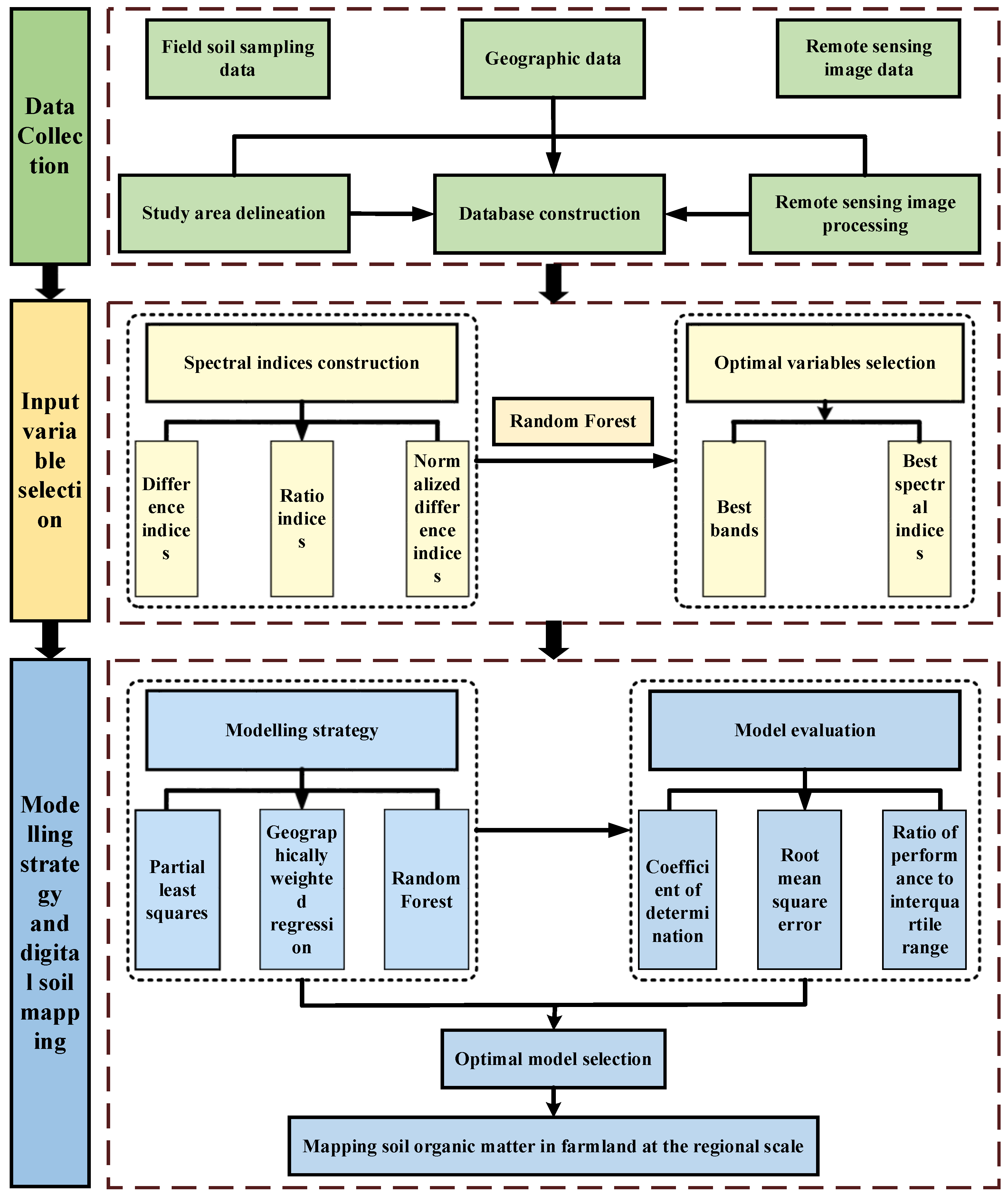
In addition, we used ArcGIS 10.2 (Environmental System Research Institute, RedLands, California, USA) to map the SOM distribution in the plough layer of cultivated land throughout the study region by using a resulting model of optimal performance. The workflow chart of this study is shown in Figure 2.

3. Results

3.1. SOM Content of the Soil Sampling Points

We calculated the descriptive statistics for the SOM content of the whole, calibration and validation datasets (Table 2). The SOM content of the whole dataset ranged from 13.79 g kg−1 to 40.64 g kg−1 with a CV of 22.58%, which indicates the SOM spatial variability in the study area. The high SOM spatial variability in this study region may improve the accuracy of the estimated SOM [10]. Based on Levene’s analysis of variance (ANOVA) test (p = 0.78), the significance (p) between the two datasets was 0.09 at the 5% level of significance, which suggests that the two datasets are representative. The SOM content ranges in the calibration dataset and validation dataset were 13.79–40.64 g kg−1 and 14.20–36.63 g kg−1, respectively. The CV values for the calibration dataset and validation dataset were 23.29% and 20.47%, respectively, with SD values of 5.89 g kg−1 and 5.56 g kg−1, respectively.

3.2. Characterization of the Soil Spectral Reflectance from Satellite Images

For the single-temporal spectral indices (Figure S1a), the concavity of the multispectral curve was consistent with the absorption properties of the soil hyperspectral curve. There were two main absorption valleys in the soil spectral reflectance near 1400 nm and 1900 nm, which corresponded to Bands 11 and 12, respectively, of the Sentinel-2A images, and these absorption valleys were strongly influenced by moisture [20]. Therefore, the construction of multitemporal spectral indices by using these bands can effectively eliminate the effect of soil moisture. As shown in Figure S1b, constructing ratios and differences in the spectral reflectance of multitemporal remote sensing images can effectively reduce the influence of soil moisture.
Figure 3 shows the reflectance spectral characteristics of the Sentinel-2A images of SOM content at the same sampling point for different soil types at different periods. Due to factors such as precipitation, crop cover, and crop residues, the SOM reflectance significantly changed in different periods, and the variation was particularly dramatic in bands 8–12, especially for yellow-brown earths. According to the Wuhan Water Resources Bulletin, Huangpi’s precipitation in 2016, 2018 and 2020 was 1597.8 mm, 1101.8 mm, and 1711.9 mm, respectively. Figure 3 shows that the soil reflectance was relatively high in the study region in 2018 because of less precipitation. The soil reflectance was relatively high with less soil moisture, which was consistent with the pattern of variation in the spectral reflectance curve and the water content measured in the laboratory [54].
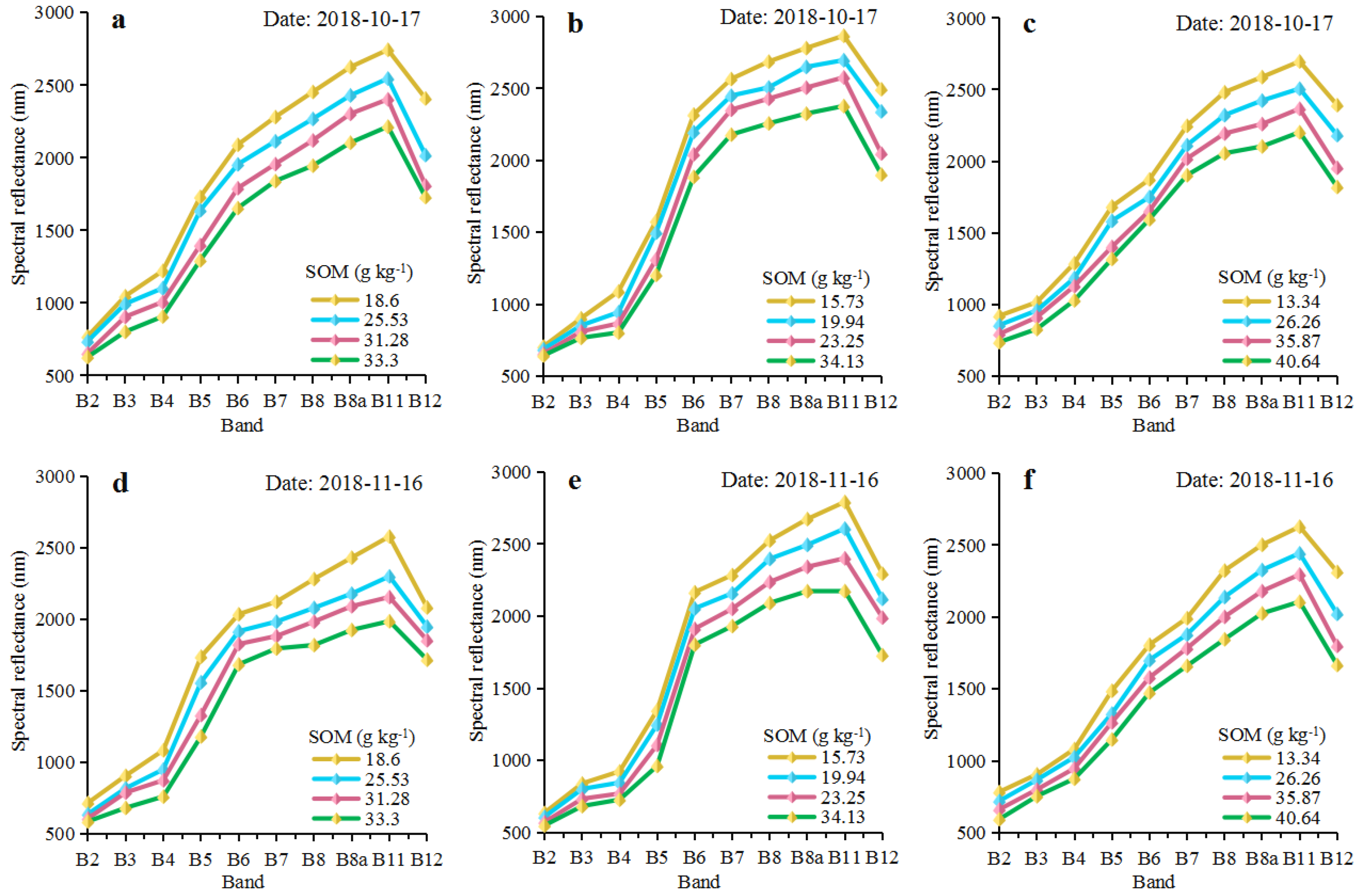
The spectral reflectance curves for different soil types with different SOM contents for the same period in 2016, 2018, and 2020 (Figure 4, Supplementary Figures S2 and S3) showed that although the seeding was completed in mid-October and the crops sprouted in mid-late November in the study area, the absorption of the red band was not significant because of the small coverage of seedlings. The trend of decreasing overall reflectance with increasing SOM was preserved in the multitemporal images across the three years, which is consistent with the results measured in the laboratory [20]. Based on the spectral changes in different SOM content reflectance spectra from the multitemporal Sentinel-2A images from the three years, the spectral curves differed more obviously in bands 8–12. However, changes in the reflectance spectral curves for different SOM contents in different soil types during the same times were observed, with the most significant changes in yellow-brown earths; these differences may be positively correlated with soil fertility levels [19,20].
Supplementary Figure S4 shows the spectral curves of the same soil sample after moisture blending and resampling according to the Sentinel-2A band range. With increasing soil water content, an overall decreasing trend in soil reflectance was observed. The changes in water content had a greater effect on soil reflectance in bands 8, 8a, 11, and 12 than in bands 2, 3, 4, 5, 6, and 7.

3.3. Selection of the Optimal Prediction Variables

3.3.1. Optimal Prediction Variables for the Single-Temporal Images

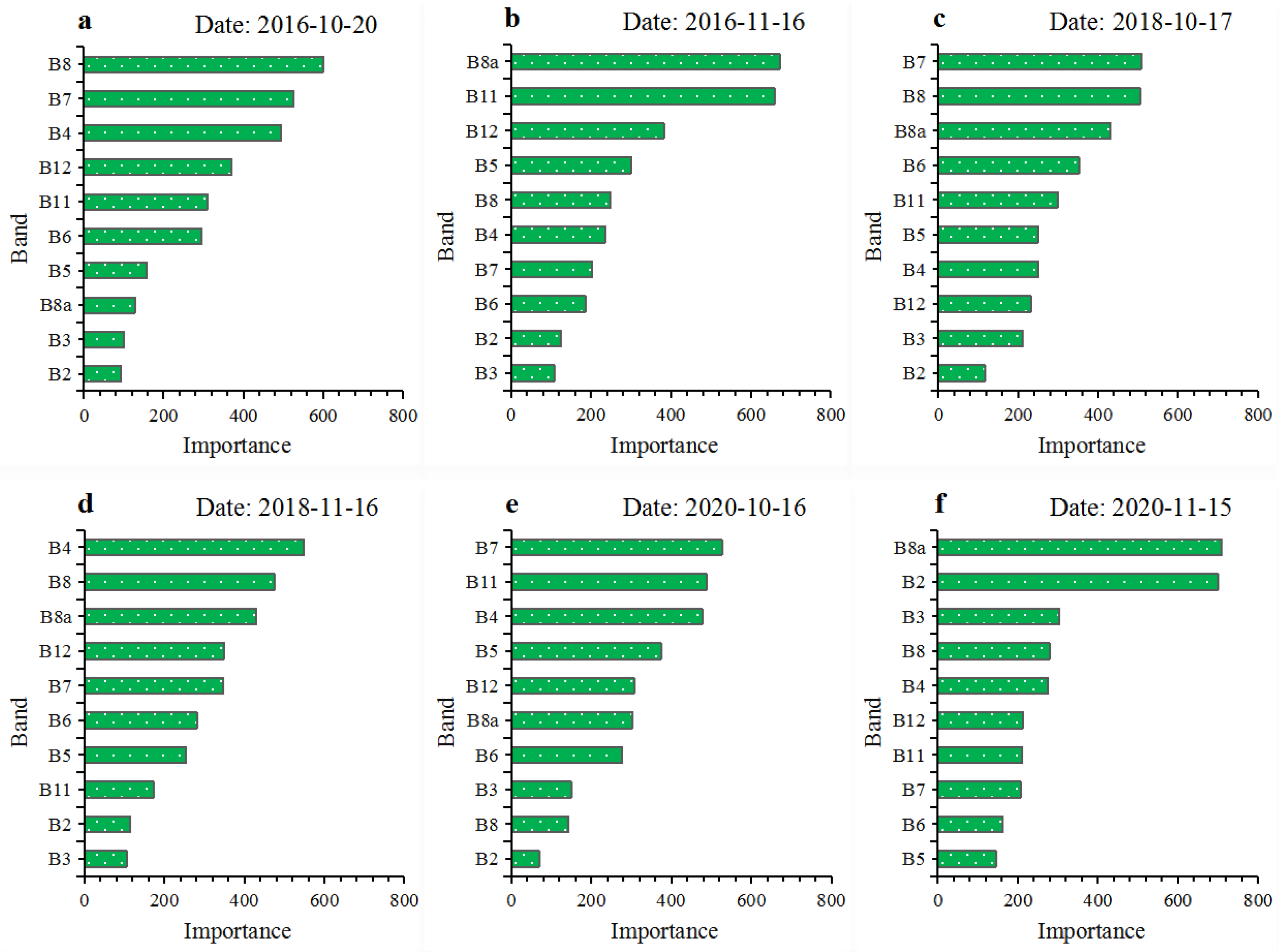
Using the spectral reflectance of the single-temporal images as prediction variables, RF was used to obtain the importance ranking of each band to estimate the SOM (Figure 5). The bands with a relatively high importance for the 20 October 2016 and 16 November 2016 images were (B8, B7, B4, B12, and B11) and (B8a, B11, B12, B5, and B8), respectively, with a total explanation level of 74.8% and 75.47%, respectively. The bands with relatively high importance for the 17 October 2018 and 16 November 2018 images were (B7, B8, B8a, B6, and B11) and (B4, B8, B8a, B12, and B7), respectively, with a total explanation level of 66.34% and 69.81%, respectively. The bands with relatively high importance for the 16 October 2020 and 15 November 2020 images were (B7, B11, B4, B5, and B12) and (B8a, B2, B3, B8, and B4), respectively, with a total explanation level of 69.71% and 72.09%, respectively.
The best bands and spectral indices of the single-temporal images were utilized as prediction variables, and the RF algorithm was selected to generate a ranking of the relative importance of the best bands and spectral indices to estimate the SOM (Supplementary Table S1). The top 10 independent variables were selected as the final prediction variables according to the level of SOM explanation greater than 70%. The bands and spectral indices selected for the 20 October 2016 and 16 November 2016 images were (B7, B8, B11, B4, B12, D412, ND118, D84, D128, and D47) and (B11, B8a, B5, B12, B8, D125, D58a, D88a, D8a12, and D58), respectively, with overall SOM explanation levels of 74.95% and 75.39%, respectively. The bands selected for the 17 October 2018 and 16 November 2018 images were (B6, B7, B8, B8a, B11, D611, D8a6, D68, D76, and ND78a) and (B4, B12, B8a, B8, B7, D124, D48, D78a, R87, and ND78), respectively, with overall SOM explanation levels of 75.93% and 75.46%, respectively. The bands selected for the 16 October 2020 and 15 November 2020 images were (B7, B11, B5, B4, B12, D124, D411, D74, D1112, and ND411) and (B8, B7, B8a, B4, B6, D8a4, D84, D74, R86, and ND86), respectively, with overall SOM explanation levels of 73.97% and 74.68%, respectively.
The GWR and PLS models are linear regression models, so the multicollinearity between variables needs to be eliminated through a significance test before modelling. For the GWR and PLS models, at a significance level of 5%, the variables selected for the 20 October 2016 and 16 November 2016 images were (B7, B8, B11, B4, B12 and ND118) and (B11, B8a, B5, B12, and B8), respectively. The variables selected for the 17 October 2018 and 16 November 2018 images were (B6, B7, B8, B8a, B11, and ND78a) and (B4, B7, B8, B8a, B12, R87, and ND78), respectively. The variables selected for the 16 October 2020 and 15 November 2020 images were (B4, B5, B7, B11, B12, and ND411) and (B8, B4, B8a, B7, B6, R86, and ND86), respectively.

3.3.2. Optimal Prediction Variables for the Double-Temporal Images

Using the spectral reflectance of the double-temporal images as prediction variables, the RF algorithm was employed to obtain the importance ranking of each band to estimate the SOM (Supplementary Figure S5). The first seven independent variables were selected as the final prediction variables according to a level of SOM explanation greater than 65%. The bands with relatively high importance in the double-temporal images from 2016, 2018, and 2020 were (B8, B4, B7, B12, and B11) for the 20 October 2016 image and (B11 and B8a) for the 16 November 2016 image; (B8, B6, B7, B5, B8a, and B11) for the 17 October 2018 image and (B4) for the 16 November 2018 image; and (B7, B4, B11, B5, and B8a) for the 16 October 2020 image and (B8 and B4) for the 15 November 2020 image, respectively; and the total SOM explanation levels were 66.69%, 65.45%, and 65.85%, respectively.
The best bands and spectral indices in the double-temporal images were selected as prediction variables to obtain the order of importance of the best bands and spectral indices to estimate the SOM, and the top 10 independent variables were selected as the final inputs according to an SOM explanation level greater than 70% (Table 3). The variables of relatively high importance in the double-temporal image from 2016, 2018, and 2020 were (B8, B4, B7, B12, and B11) for the 20 October 2016 image, (B11 and B8a) for the 16 November 2016 image, (D1020-1116_48a, R1020-1116_411, and ND1020-1116_411); (B8, B6, B7, B5, B8a, and B11) for the 17 October 2018 image, (B4) for the 16 November 2018 image, (D1116-1017_48, D1017-1116_74, and D1116-1017_411); and (B7, B4, B11, B5, and B8a) for the 16 October 2020 image, (B8 and B4) for the 15 November 2020 image, (D1115-1016_84, D1115-1016_47, and ND1016-1115_48), respectively; and the total SOM explanation levels were 70.49%, 77.85%, and 71.60%, respectively.
The independent variables of the PLS and GWR models were further selected with significance testing based on selecting the best variables in the double-temporal images by using the RF algorithm. At a significance level of 5%, the variables of relatively high importance in the double-temporal images from 2016, 2018, and 2020 were (B8, B4, B7, B12, and B11) for the 20 October 2016 image, (B11 and B8a) for the 16 November 2016 image, and (ND1020-1116_411); (B8, B6, B7, B5, B8a, and B11) for the 17 October 2018 image and (B4) for the 16 November 2018 image; and (B7, B4, B11, B5, and B8a) for the 16 October 2020 image, (B8 and B4) for the 15 November 2020 image, and (ND1016-1115_48), respectively.

3.4. Analysis of the SOM Estimation Model for the Single-Temporal Images

To verify the effect of the single-temporal images from the Sentinel-2A satellite on model performance, we constructed 36 PLS, GWR, and RF models to estimate SOM by using single-temporal images in 2016, 2018, and 2020 (Supplementary Table S2). In the PLS model, when using the full spectrum as prediction variables, the highest model accuracy was achieved with the 17 October 2018 image (R2val = 0.38, RMSEval = 2.98, and RPIQval = 2.31). Based on the optimal bands and spectral indices for the prediction variables, the Sentinel-2A image from 15 November 2020 was better than that of other periods for the SOM estimation, with R2val = 0.47, RMSEval = 2.63, and RPIQval = 2.62. In the GWR models, the best predictions (R2val = 0.45, RMSEval = 2.70, and RPIQval = 2.55) were provided by using the 17 October 2018 image based on the full spectrum data. When using the optimal bands and spectral indices data, the SOM estimation performance of the Sentinel-2A image for the same period in the three years was better than that of the PLS model in terms of RPIQval, with the best SOM estimation performance of the Sentinel-2A image from 17 October 2018, with R2val = 0.55, RMSEval = 2.40, and RPIQval = 2.87. Whether based on the full spectrum data or the optimal bands and spectral indices data, RF performed better than the two linear simulation methods and had the highest R2val, lowest RMSEval, and highest RPIQval values in the Sentinel-2A images for the same single periods in 2016, 2018, and 2020. Based on the full spectrum data, the model developed from the 17 October 2018 image had the best stability and accuracy (R2val = 0.50 and RPIQval = 2.77). When using the optimal bands and spectral indices as prediction variables, the best validation results were obtained for the 17 October 2018 image (R2val = 0.61 and RPIQval = 2.93).

3.5. Analysis of the SOM Estimation Model for the Double-Temporal Images

Table 4 shows the results of the SOM prediction models constructed for PLS, GWR, and RF based on the multitemporal Sentinel-2A images from 2016, 2018, and 2020. The PLS model based on the full-spectrum data as prediction variables that used the double-temporal images in 2018 provided the best predictions (R2val = 0.45, RMSEval = 2.74, and RPIQval = 2.26). When using the optimal band and spectral indices as prediction variables, the PLS model based on the double-temporal images in 2018 had the best stability and accuracy, with R2val = 0.53, RMSEval = 2.43, and RPIQval = 2.83. The GWR model outperformed the PLS model in estimating SOM content. When using the full-spectrum data as prediction variables, the model based on the double-temporal images in 2018 had the best stability and accuracy, with R2val = 0.50 and RPIQval = 2.47. Based on the best bands and spectral indices data, the multitemporal images in 2018 achieved the best estimation performance (R2val = 0.59, RMSEval = 2.37, and RPIQval = 2.91). Compared with the PLS and GWR models, the RF model had the highest accuracy in estimating SOM content. The model based on the full-spectrum data as prediction variables in 2018 had the best stability and accuracy (R2val = 0.55, RMSEval = 2.28, and RPIQval = 3.02). When using the optimal bands and spectral indices data as prediction variables, the highest validation accuracy was achieved in 2018 (R2val = 0.67 and RPIQval = 3.36).
Overall, whether using the single- or double-temporal images, the SOM estimation model developed from the optimal bands and spectral indices was more accurate than the model developed from full spectral data. In addition, the models constructed based on the double-temporal images had a better estimation performance than those based on single-temporal images. When the optimal bands and spectral indices were utilized as prediction variables, the R2val of the optimal SOM estimation model for the double-temporal images was improved by more than 30% compared with the optimal SOM inversion model for the single-temporal images. Therefore, this result indicates that the combination of optimal bands and spectral indices and multitemporal images is beneficial in reducing the influence of interference factors such as straw cover and soil moisture content on the accuracy of the SOM estimation model from remote sensing images. The RF model for the SOM estimation performed better than the GWR and PLS models, regardless of the estimating variables selected. This result reveals the ability of RF to estimate SOM. The SOM estimation based on remote sensing satellite images shows that higher spectral resolution remote sensing satellites such as Sentinel-2A have the potential to estimate regional-scale SOM contents in cultivated land (maximum R2val = 0.67).
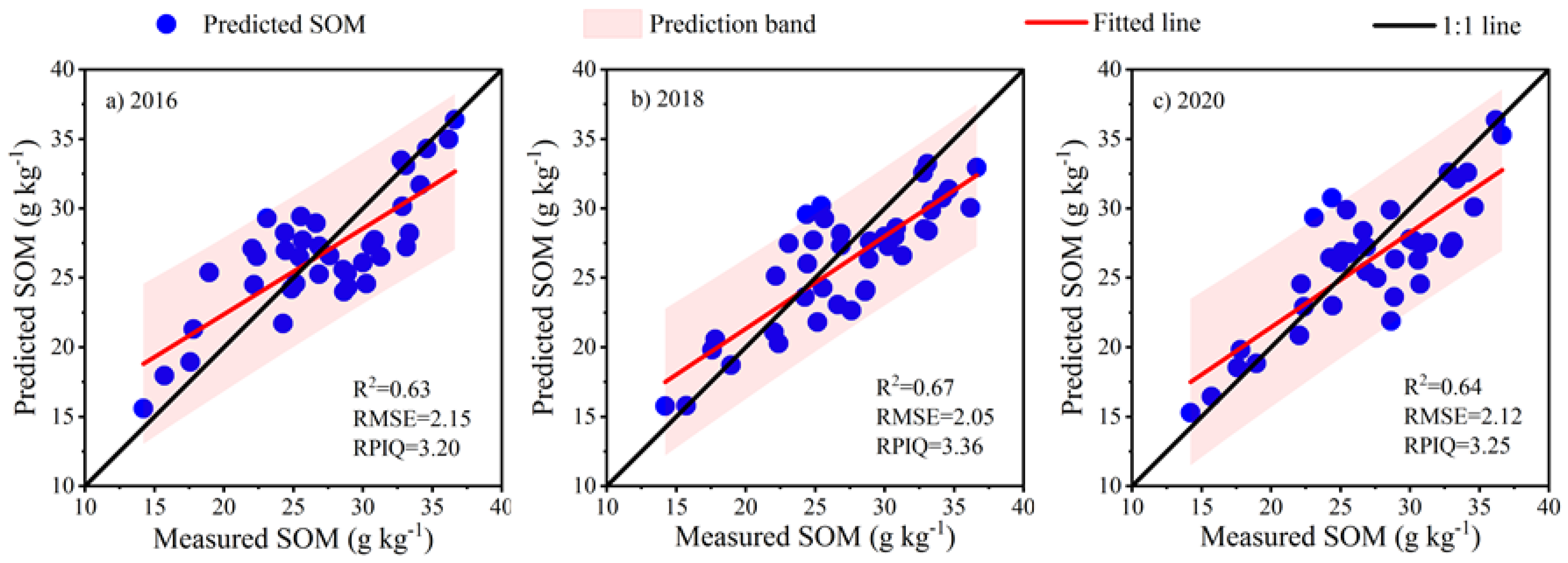
To further verify that the combination of the double-temporal images and spectral indices helped to improve the performance of the SOM estimation models, an ANOVA was conducted with RMSEval (dependent variable), the double-temporal images and the regression models (independent variables) by using the best bands and spectral indices (Supplementary Table S3). Our studies indicated that the double-temporal images that used the best band and spectral indices as prediction variables (p < 0.02) had a more significant impact on the performance of the SOM estimation models than the regression models (p < 0.05). In addition, a scatter plot between the measured and the estimated SOM from the RF model based on the double-temporal images in 2018 that used the optimal bands and spectral indices as the prediction variables is shown in Figure 6. When using the optimal bands and spectral indices as prediction variables, the regression lines to estimate the SOM content with the RF model based on the double-temporal images in 2018 were near the 1:1 line, which indicated that even though high contents of SOM (≥25 g kg−1) were underestimated, the correlation between the measured and the estimated SOM was strong (Figure 6).

3.6. SOM Mapping in the Plough Layer for the Cultivated Land throughout the Study Area

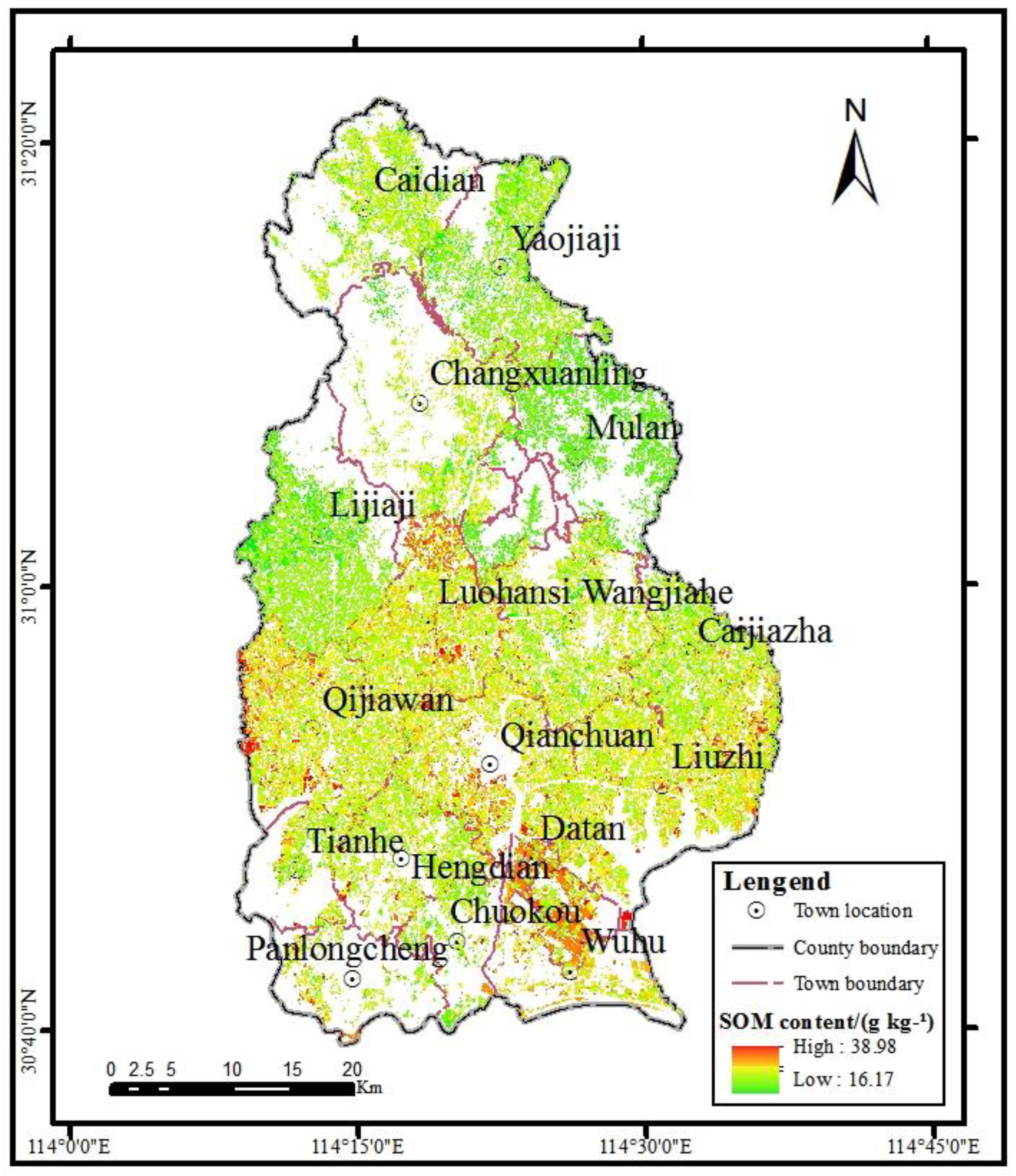
To validate the applicability of our approaches, we estimated the SOM contents by using the model with the best stability and accuracy (highest R2val, largest RPIQval, and lowest RMSEval) and mapped the SOM distribution in the plough layer for the cultivated land throughout the study area (Figure 7). The SOM content ranged from 16.17 to 36.98 g kg−1, and the area with contents between 25.36 and 28.12 g kg−1 was 388.53 km2, with a percentage of 40.91% (Table 5), which indicates a better soil fertility in this study area. As shown in Figure 7, the SOM distribution in the plough layer for cultivated land throughout the study area exhibits a pattern of high SOM contents in the south-central part and low SOM contents in the northern part. The south-central part of the study area is a lake with a surrounding plain, which has high SOM contents and widely distributed fluvo-aquic soils and yellow-brown earths with high SOM contents. The northern area is hilly and mountainous, with serious soil erosion, poor soil fertility, and low SOM contents. Because of the lack of data, we could not validate the SOM maps, but the high R2val and RPIQval and low RMSEval ensure the applicability of the SOM maps.

4. Discussion

It has been shown that SOM has a remarkable negative relationship with soil spectral reflectance. It is feasible to estimate SOM accurately at laboratory and field scales by using portable spectrometers [55,56]. However, because of the influences of soil moisture, vegetation cover, crop residues, and the spectral resolution and spatial resolution of different sensors, few studies have been conducted to estimate SOM using airborne hyperspectral sensors. Compared to ground and airborne remote sensing, satellite remote sensing has a relatively high temporal resolution [57]. Therefore, multitemporal satellite remote sensing images may be an important way to rapidly estimate the content of SOM over a large area, particularly where the land surface is temporarily or permanently exposed [12]. In recent years, scholars worldwide have made progress in the use of satellite remote sensing images to predict the SOM content [15,17]. However, many studies have used only spectral data from single-period images to predict SOM, which limits the accuracy of the estimation models [58]. The introduction of temporal information compensates for the lack of information in single-temporal images and allows a more comprehensive extraction of pixel information common to multiple images [59]. Additionally, multitemporal images can also be characterized by the constructed multitemporal spectral indices to characterize the interactivity of the factors, which can achieve the goal of reducing the effect of the factors and thus improve the accuracy of SOM estimation models [54]. Our studies show that the stability and accuracy were better for the multitemporal Sentinel-2A image estimation model than for the single-period Sentinel-2A image estimation model (Table S2 and Table 4).
It is not feasible to select all band combinations to construct spectral indices to estimate soil properties because of the large amount of spectral data that is processed [60]. In this study, we employed the RF model to select the best bands to construct spectral indices, which can reduce the highly redundant spectral data. Our results showed that the SOM spectrum was especially sensitive throughout the visible, near-infrared, and shortwave infrared regions (400 to 2500 nm), with unique spectral response bands that are consistent with previous studies [61,62]. Among them, the spectral data were dominated by the darkness of soil chromophores and humic acids [19,58]. In this study, for most single- and double-temporal image estimation models, bands 4, 7, 8, 11, 12 and D, R, and ND were selected as the best prediction variables (Table S1 and Table 3), which is consistent with the spectral response bands identified in previous SOM studies [19,20].
The use of spectral indices as predictors is more beneficial in eliminating the effect of environmental factors such as tillage practices, crop residue and soil moisture content than the use of reflectance data as predictors [54,63]. D was more suitable for conditions with lower soil moisture and minimal crop residue. R can effectively reduce the disturbance of the SOM spectral reflectance by soil moisture. The model validation results based on multitemporal Sentinel-2A images from 2016, 2018, and 2020 showed that the performance was better for the 2018 image estimation model than for the 2016 and 2020 image estimation models (Table S2 and Table 4). According to data from the Wuhan City Statistical Yearbook, there was low straw cover and soil moisture in 2018 in the study area, which produced a better accuracy. Furthermore, SOM is relatively stable and gradually changes; thus, we can utilize remote sensing images from periods when there is less crop residue in farmland to estimate the SOM content [20]. Our results confirm the potential of using spectral indices as predictor variables to construct SOM spectral inversion models (Table S2 and Table 4).
Different modelling techniques can affect the performance of SOM estimation models. In this study, the RF model was more accurate than the PLS and GWR models in almost all cases, and the GWR model was more accurate than the PLS model (Table S2 and Table 4). The accuracy of the optimal SOM estimation model (in the RF model that used the multitemporal images from 2018, R2val = 0.67, and RPIQval = 3.36) is basically consistent with the results of most previous studies [20,64]. Combined with previous studies [65,66], our study further confirms the advantages of the RF model for SOM estimation and that the RF model had significant differences in the methodological properties from the PLS and GWR models. Additionally, the RF model considered the useful nonlinear information between SOM and soil spectral data, so it achieved a higher SOM estimation accuracy than the PLS and GWR models. In contrast, the PLS and GWR models identified only linear relationships between SOM and soil spectral data. In addition, the disadvantage of both the PLS and GWR models was the long computation time, particularly when handling high-dimensional data.
The spectral properties of soil samples tend to exhibit regional variability. We estimated the SOM content in the plough layer for cultivated land in Huangpi District based on multitemporal remote sensing images in the bare soil period; therefore, our results may not be suitably comparable with other regions around the globe. In particular, the SOM estimation model built by remote sensing images in this study may not be suitable for areas where the exposure of tilled soil is nonexistent or short due to the use of continuous cropping systems on cropland. Additionally, the SOM estimation model may also not be suitable for other types of land cover or different vegetation communities. Furthermore, although the SOM spectral profile differed among the soil types, it had a minimal effect on the correlation between the SOM contents and their response bands. Whether the introduction of soil type variables can improve the accuracy of SOM estimation through remote sensing images will need to be explored in depth.

5. Conclusions

In this study, we employed multispectral Sentinel-2A images over 3 years (2016, 2018, and 2020) to construct spectral indices as SOM prediction variables and explored the potential of combining three regression methods, specifically, PLS, GWR, and RF, for regional SOM estimation in the plough layer for cultivated land. The models constructed with multitemporal images had better accuracy than those constructed with single-temporal images. The RF algorithm provided more efficient prediction variables for SOM estimation by reducing redundant spectral reflectance data and allowing the optimization of the SOM estimation model. In addition, the prediction accuracy was usually better for the SOM estimation models that used the optimal bands and spectral indices than for the models based on full spectral data. The model accuracy and stability of the multitemporal remote sensing images based on the optimal bands and spectral indices were the highest for 2018 among the analysed years (R2val: 0.53–0.67 and RPIQval: 2.83–3.36) because of less precipitation and lower straw cover in 2018 than in 2016 and 2020. The nonlinear model (RF) outperformed the linear correction models (PLS and GWR) in the remote sensing images for all periods, even with the relatively few soil sample points applied in this study. The optimal RF model based on the multitemporal remote sensing images from 2018 that used the optimal bands and spectral indices as prediction variables was preferred to accurately estimate the SOM content in the plough layer for cultivated land throughout the study area, with a validated R2val of 0.67 and an RPIQval of 3.36. The estimated SOM content in the plough layer for cultivated land throughout the study area ranged from 16.17 to 36.98 g kg−1 and exhibited an increasing trend from north to south. This spatial information can help to improve the prediction accuracy of soil attributes estimated from multispectral images. Our study confirms the effectiveness of multitemporal Sentinel-2A spectral imaging for the rapid estimation of SOM in the plough layer for cultivated land at the regional scale and demonstrates that the RF model is an effective tool for handling complex datasets.
In the current study, we designed a framework that combined multitemporal remote sensing imagery and RF for the rapid estimation of SOM content, which can improve the accuracy of quantitative SOM content estimation at the regional scale and provide a reference for future field soil sampling and to achieve high-accuracy SOM prediction in similar areas. However, the analysis of the factors that affect the spatial heterogeneity of SOM content in this study was insufficient. In practical agricultural production, factors such as topography, climate, cropping patterns, and land-use changes can influence the distribution of SOM content. Therefore, to investigate the interaction mechanism between both the natural environment and socioeconomic factors and SOM content, the focus of our next in-depth study will be whether it can further improve the prediction accuracy of SOM.

Supplementary Materials

The following are available online at https://www.mdpi.com/article/10.3390/agriculture13010008/s1, Figure S1: Illustration of the spectral indices constructed by (a) single-temporal images and (b) multitemporal images, Figure S2: Spectral reflectance data for different soil types with different SOM contents in the same period in 2016: (a) and (d) fluvo-aquic soils; (b) and (e) yellow-brown earths; (c) and (f) paddy soils, Figure S3: Spectral reflectance data for different soil types with different SOM contents in the same period in 2020: (a) and (d) fluvo-aquic soils; (b) and (e) yellow-brown earths; (c) and (f) paddy soils, Figure S4: Soil spectral curves for the same SOM content at different moisture contents, Figure S5: Importances of the bands in the SOM estimation model based on double-temporal images: (a) 2016; (b) 2018; (c) 2020, Table S1: Importance of optimal bands and spectral indices for SOM estimation using single-temporal images, Table S2: Statistical results of the three different modelling algorithms using single-temporal images based on full spectrum data and the optimum bands and spectral indices in 2016, 2018, and 2020, Table S3: Analysis of variance in the RMSEval values of double-temporal images and regression models based on the optimal bands and spectral indices.

Author Contributions

Methodology, L.W.; data curation, L.W.; writing—original draft preparation, L.W.; writing—review and editing, Y.Z.; funding acquisition, Y.Z. All authors have read and agreed to the published version of the manuscript.

Funding

This research was funded by the National Natural Science Foundation of China (No. 42171061) and the Special Foundation for National Science and Technology Basic Research Program of China (No. 2021FY100505). The APC was funded by the National Natural Science Foundation of China and the Special Foundation for National Science and Technology Basic Research Program of China.

Institutional Review Board Statement

Not applicable.

Conflicts of Interest

The authors declare no conflict of interest.

References

  1. Wu, C.; Liu, G.; Huang, C.; Liu, Q. Soil Quality Assessment in Yellow River Delta: Establishing a Minimum Data Set and Fuzzy Logic Model. Geoderma 2019, 334, 82–89. [Google Scholar] [CrossRef]
  2. Luo, C.; Zhang, X.; Wang, Y.; Men, Z.; Liu, H. Regional Soil Organic Matter Mapping Models Based on the Optimal Time Window, Feature Selection Algorithm and Google Earth Engine. Soil Tillage Res. 2022, 219, 105325. [Google Scholar] [CrossRef]
  3. Lin, L.; Han, S.; Zhao, P.; Li, L.; Zhang, C.; Wang, E. Influence of Soil Physical and Chemical Properties on Mechanical Characteristics under Different Cultivation Durations with Mollisols. Soil Tillage Res. 2022, 224, 105520. [Google Scholar] [CrossRef]
  4. Bradford, M.; Wood, S.; Addicott, E.; Fenichel, E.; Fields, N.; Gonzlez-Rivero, J.; Jevon, F.; Maynard, D.; Oldfield, E.; Polussa, A.; et al. Quantifying Microbial Control of Soil Organic Matter Dynamics at Macrosystem Scales. Biogeochemistry 2021, 156, 19–40. [Google Scholar] [CrossRef]
  5. Buckeridge, K.; Creamer, C.; Whitaker, J. Deconstructing the Microbial Necromass Continuum to Inform Soil Carbon Sequestration. Funct. Ecol. 2022, 36, 1396–1410. [Google Scholar] [CrossRef]
  6. Liu, J.; Xie, J.; Meng, T.; Dong, H. Organic Matter Estimation of Surface Soil Using Successive Projection Algorithm. Agron. J. 2022, 114, 1944–1951. [Google Scholar] [CrossRef]
  7. Lu, M.; Liu, Y.; Liu, G. Precise Prediction of Soil Organic Matter in Soils Planted with a Variety of Crops through Hybrid Methods. Comput. Electron. Agric. 2022, 200, 107246. [Google Scholar] [CrossRef]
  8. Wang, Z.; Du, Z.; Li, X.; Bao, Z.; Zhao, N.; Yue, T. Incorporation of High Accuracy Surface Modeling into Machine Learning to Improve Soil Organic Matter Mapping. Ecol. Indic. 2021, 129, 107975. [Google Scholar] [CrossRef]
  9. Song, Y.Q.; Yang, L.A.; Li, B.; Hu, Y.M.; Wang, A.L.; Zhou, W.; Cui, X.S.; Liu, Y.L. Spatial Prediction of Soil Organic Matter Using a Hybrid Geostatistical Model of an Extreme Learning Machine and Ordinary Kriging. Sustainability 2017, 9, 754. [Google Scholar] [CrossRef] [Green Version]
  10. Hong, Y. Application of Fractional-Order Derivative in the Quantitative Estimation of Soil Organic Matter Content through Visible and near-Infrared Spectroscopy. Geoderma 2018, 337, 758–769. [Google Scholar] [CrossRef]
  11. Asrar, G. Theory and Applications of Optical Remote Sensing. Trans. Inst. Br. Geogr. 1989, 18, 159–160. [Google Scholar]
  12. Zhai, M. Inversion of Organic Matter Content in Wetland Soil Based on Landsat 8 Remote Sensing Image. J. Vis. Commun. Image Represent. 2019, 64, 102645. [Google Scholar] [CrossRef]
  13. Fu, C.; Xiong, H.; Tian, A. Study on the Effect of Fractional Derivative on the Hyperspectral Data of Soil Organic Matter Content in Arid Region. J. Spectrosc. 2019, 2019, 7159317. [Google Scholar] [CrossRef] [Green Version]
  14. Gu, X.; Wang, Y.; Sun, Q.; Yang, G.; Zhang, C. Hyperspectral Inversion of Soil Organic Matter Content in Cultivated Land Based on Wavelet Transform. Comput. Electron. Agric. 2019, 167, 105053. [Google Scholar] [CrossRef]
  15. Sun, M.; Li, Q.; Jiang, X.; Ye, T.; Li, X.; Niu, B. Estimation of Soil Salt Content and Organic Matter on Arable Land in the Yellow River Delta by Combining UAV Hyperspectral and Landsat-8 Multispectral Imagery. Sensors 2022, 22, 3990. [Google Scholar] [CrossRef]
  16. Castaldi, F.; Casa, R.; Castrignano, A.; Pascucci, S.; Palombo, A.; Pignatti, S. Estimation of Soil Properties at the Field Scale from Satellite Data: A Comparison between Spatial and Non-Spatial Techniques. Eur. J. Soil Sci. 2014, 65, 842–851. [Google Scholar] [CrossRef]
  17. Li, X.; Zhang, F.; Wang, X.P. Study on Differential-Based Multispectral Modeling of Soil Organic Matter in Ebinur Lake Wetland. Spectrosc. Spectr. Anal. 2019, 039, 535–542. [Google Scholar]
  18. Wang, X.; Zhang, F.; Kung, H.T.; Johnson, V.C. New Methods for Improving the Remote Sensing Estimation of Soil Organic Matter Content (SOMC) in the Ebinur Lake Wetland National Nature Reserve (ELWNNR) in Northwest China. Remote Sens. Environ. 2018, 218, 104–118. [Google Scholar] [CrossRef]
  19. Liu, H.; Zhang, M.; Yang, H.; Zhang, X.; Meng, X.; Li, H.; Tang, H. Invertion of Cultivated Soil Organic Matter Content Combining Multi-Spectral Remote Sensing and Random Forest Algorithm. Trans. Chin. Soc. Agric. Eng. 2020, 36, 134–140. [Google Scholar]
  20. Dou, X.; Wang, X.; Liu, H.; Zhang, X.; Cui, Y. Prediction of Soil Organic Matter Using Multi-Temporal Satellite Images in the Songnen Plain, China. Geoderma 2019, 356, 113896. [Google Scholar] [CrossRef]
  21. Yu, Q.; Yao, T.; Lu, H.; Feng, W.; Xue, Y.; Liu, B. Improving Estimation of Soil Organic Matter Content by Combining Landsat 8 OLI Images and Environmental Data: A Case Study in the River Valley of the Southern Qinghai-Tibet Plateau. Comput. Electron. Agric. 2021, 185, 106144. [Google Scholar] [CrossRef]
  22. Xu, S.; Zhao, Y.; Wang, M.; Shi, X. Comparison of Multivariate Methods for Estimating Selected Soil Properties from Intact Soil Cores of Paddy Fields by Vis-NIR Spectroscopy. Geoderma 2018, 310, 29–43. [Google Scholar] [CrossRef]
  23. Ma, Y.; Jiang, Q.G.; Meng, Z.G.; Liu, H.X. Black Soil Organic Matter Content Estimation Using Hybrid Selection Method Based on RF and GABPSO. Spectrosc. Spectr. Anal. 2018, 38, 181–187. [Google Scholar]
  24. Xie, S.; Li, Y.; Wang, X.; Liu, Z.; Ma, K.; Ding, L. Research on Estimation Models of the Spectral Characteristics of Soil Organic Matter Based on the Soil Particle Size. Spectrochim. Acta Part A Mol. Biomol. Spectrosc. 2021, 260, 119963. [Google Scholar] [CrossRef]
  25. Yang, M.; Xu, D.; Chen, S.; Li, H.; Shi, Z. Evaluation of Machine Learning Approaches to Predict Soil Organic Matter and PH Using Vis-NIR Spectra. Sensors 2019, 19, 263. [Google Scholar] [CrossRef] [Green Version]
  26. Hong, Y.; Chen, S.; Zhang, Y.; Chen, Y.; Yu, L.; Liu, Y.; Liu, Y.; Cheng, H.; Liu, Y. Rapid Identification of Soil Organic Matter Level via Visible and Near-Infrared Spectroscopy: Effects of Two-Dimensional Correlation Coefficient and Extreme Learning Machine. Sci. Total Environ. 2018, 644, 1232–1243. [Google Scholar] [CrossRef]
  27. Chen, D.; Chang, N.; Xiao, J.; Zhou, Q.; Wu, W. Mapping Dynamics of Soil Organic Matter in Croplands with MODIS Data and Machine Learning Algorithms. Sci. Total Environ. 2019, 669, 844–855. [Google Scholar] [CrossRef]
  28. Zhang, S.; Lu, X.; Nie, G.; Li, Y.; Shao, Y.; Tian, Y.; Fan, L.; Zhang, Y. Estimation of Soil Organic Matter in Coastal Wetlands by SVM and BP Based on Hyperspectral Remote Sensing. Spectrosc. Spectr. Anal. 2020, 40, 556–561. [Google Scholar]
  29. Jiao, C.; Zheng, G.; Xie, X.; Cui, X.; Shang, G. Prediction of Soil Organic Matter Using Visible-Short Near-Infrared Imaging Spectroscopy. Spectrosc. Spectr. Anal. 2020, 40, 3277–3281. [Google Scholar]
  30. Schmidhuber, J. Deep Learning in Neural Networks: An Overview. Neural Netw. 2015, 61, 85–117. [Google Scholar] [CrossRef] [Green Version]
  31. Mountrakis, G.; Im, J.; Ogole, C. Support Vector Machines in Remote Sensing: A Review. ISPRS J. Photogramm. Remote Sens. 2011, 66, 247–259. [Google Scholar] [CrossRef]
  32. Huang, G.; Zhu, Q.; Siew, C. Extreme Learning Machine: Theory and Applications. Neurocomputing 2006, 70, 489–501. [Google Scholar] [CrossRef]
  33. Kadiyala, A.; Kumar, A. Applications of Python to Evaluate the Performance of Decision Tree-Based Boosting Algorithms. Environ. Prog. Sustain. Energy 2018, 37, 618–623. [Google Scholar] [CrossRef]
  34. Breiman, L. Random Forests. Mach. Learn. 2001, 45, 5–32. [Google Scholar] [CrossRef] [Green Version]
  35. Pouladi, N.; Møller, A.B.; Tabatabai, S.; Greve, M.H. Mapping Soil Organic Matter Contents at Field Level with Cubist, Random Forest and Kriging. Geoderma 2019, 342, 85–92. [Google Scholar] [CrossRef]
  36. Nowkandeh, S.M.; Noroozi, A.A.; Homaee, M. Estimating Soil Organic Matter Content from Hyperion Reflectance Images Using PLSR, PCR, MinR and SWR Models in Semi-Arid Regions of Iran. Environ. Dev. 2018, 25, 23–32. [Google Scholar] [CrossRef]
  37. Chen, L.; Ren, C.; Wang, Y.; Zhang, B.; Wang, Z.; Li, L. A Comparative Assessment of Geostatistical, Machine Learning, and Hybrid Approaches for Mapping Topsoil Organic Carbon Content. ISPRS Int. J. Geo-Inf. 2019, 8, 174. [Google Scholar] [CrossRef] [Green Version]
  38. FAO. World Reference Base for Soil Resources; Food and Agriculture Organization of the United Nations: Rome, Italy, 1998. [Google Scholar]
  39. Nelson, D.W.; Sommers, L.E. Total Carbon, Organic Carbon and Organic Matter. In Methods of Soil Analysis: Part 2 Chemical and Microbial Properties; Academic Press: Cambridge, MA, USA, 1982; pp. 552–553. [Google Scholar]
  40. Zhu, C.; Zhang, Z.; Wang, H.; Wang, J.; Yang, S. Assessing Soil Organic Matter Content in a Coal Mining Area through Spectral Variables of Different Numbers of Dimensions. Sensors 2020, 20, 1795. [Google Scholar] [CrossRef] [Green Version]
  41. Lin, C.; Zhu, A.; Wang, Z.; Wang, X.; Ma, R. The Refined Spatiotemporal Representation of Soil Organic Matter Based on Remote Images Fusion of Sentinel-2 and Sentinel-3. Int. J. Appl. Earth Obs. Geoinf. 2020, 89, 102094. [Google Scholar] [CrossRef]
  42. Zhou, W.; Yang, H.; Xie, L.; Li, H.; Yue, T. Hyperspectral Inversion of Soil Heavy Metals in Three-River Source Region Based on Random Forest Model. Catena 2021, 202, 105222. [Google Scholar] [CrossRef]
  43. Scornet, E. Random Forests and Kernel Methods. IEEE Trans. Inf. Theory 2016, 62, 1485–1500. [Google Scholar] [CrossRef] [Green Version]
  44. Molinaro, A.; Simon, R.; Pfeiffer, R. Prediction Error Estimation: A Comparison of Resampling Methods. Bioinformatics 2005, 21, 3301–3307. [Google Scholar] [CrossRef] [PubMed] [Green Version]
  45. Wang, X.; Yang, C.; Zhou, M. Partial Least Squares Improved Multivariate Adaptive Regression Splines for Visible and Near-Infrared-Based Soil Organic Matter Estimation Considering Spatial Heterogeneity. Appl. Sci. 2021, 11, 566. [Google Scholar] [CrossRef]
  46. Rasoolimanesh, S.M.; Ringle, C.M.; Sarstedt, M.; Olya, H. The Combined Use of Symmetric and Asymmetric Approaches: Partial Least Squares-Structural Equation Modeling and Fuzzy-Set Qualitative Comparative Analysis. Int. J. Contemp. Hosp. Manag. 2021, 33, 1571–1592. [Google Scholar] [CrossRef]
  47. Sun, W.; Liu, S.; Zhang, X.; Li, Y. Estimation of Soil Organic Matter Content Using Selected Spectral Subset of Hyperspectral Data. Geoderma 2022, 409, 115653. [Google Scholar] [CrossRef]
  48. Li, H.D.; Xu, Q.S.; Liang, Y.Z. LibPLS: An Integrated Library for Partial Least Squares Regression and Linear Discriminant Analysis. Chemom. Intell. Lab. Syst. 2018, 176, 34–43. [Google Scholar] [CrossRef]
  49. Shen, L.; Gao, M.; Yan, J.; Li, Z.; Leng, P.; Yang, Q.; Duan, S. Hyperspectral Estimation of Soil Organic Matter Content Using Different Spectral Preprocessing Techniques and PLSR Method. Remote Sens. 2020, 12, 1206. [Google Scholar] [CrossRef] [Green Version]
  50. Li, Z.; Fotheringham, A.S. Computational Improvements to Multi-Scale Geographically Weighted Regression. Int. J. Geogr. Inf. Sci. 2020, 34, 1378–1397. [Google Scholar] [CrossRef]
  51. Comber, A. Hyper-Local Geographically Weighted Regression: Extending GWR through Local Model Selection and Local Bandwidth Optimization. J. Spat. Inf. Sci. 2018, 17, 63–84. [Google Scholar] [CrossRef]
  52. Costa, E.M.; Tassinari, W.; Pinheiro, H.; Beutler, S.J.; Anjos, L.D. Mapping Soil Organic Carbon and Organic Matter Fractions by Geographically Weighted Regression. J. Environ. Qual. 2018, 47, 718–725. [Google Scholar] [CrossRef]
  53. Zeraatpisheh, M.; Ayoubi, S.; Jafari, A.; Finke, P. Comparing the Efficiency of Digital and Conventional Soil Mapping to Predict Soil Types in a Semi-Arid Region in Iran. Geomorphology 2017, 285, 186–204. [Google Scholar] [CrossRef]
  54. Zhang, X.; Dou, X.; Xie, Y.; Liu, H.; Wang, N.; Wang, X.; Pan, Y. Remote Sensing Inversion Model of Soil Organic Matter in Farmland by Introducing Temporal Information. Trans. Chin. Soc. Agric. Eng. 2018, 34, 143–151. [Google Scholar]
  55. Bao, Y.; Meng, X.; Ustin, S.; Wang, X.; Tang, H. Vis-SWIR Spectral Prediction Model for Soil Organic Matter with Different Grouping Strategies. Catena 2020, 195, 104703. [Google Scholar] [CrossRef]
  56. Said, E.; Baroudy, A.; El-Beshbeshy, T.; Emam, M.; Lasaponara, R. Vis-NIR Spectroscopy and Satellite Landsat-8 OLI Data to Map Soil Nutrients in Arid Conditions: A Case Study of the Northwest Coast of Egypt. Remote Sens. 2020, 12, 3716. [Google Scholar]
  57. Xiao, J.; Chevallier, F.; Gomez, C.; Guanter, L.; Zhang, X. Remote Sensing of the Terrestrial Carbon Cycle: A Review of Advances over 50 Years. Remote Sens. Environ. 2019, 233, 111383. [Google Scholar] [CrossRef]
  58. Chen, S.; Zou, S.; Mao, Y.; Liang, W.; Ding, H. Inversion of Soil Organic Matter Content in Wetland Using Multispectral Data Based on Soil Spectral Reconstruction. Spectrosc. Spectr. Anal. 2018, 38, 912–917. [Google Scholar]
  59. Qiao, M.; He, X.; Cheng, X.; Li, P.; Luo, H.; Zhang, L.; Tian, Z. Crop Yield Prediction from Multi-Spectral, Multi-Temporal Remotely Sensed Imagery Using Recurrent 3D Convolutional Neural Networks. Int. J. Appl. Earth Obs. Geoinf. 2021, 102, 102436. [Google Scholar] [CrossRef]
  60. Biney, J.K.M.; Saberioon, M.; Boruvka, L.; Houska, J.; Vasat, R.; Chapman Agyeman, P.; Coblinski, J.A.; Klement, A. Exploring the Suitability of UAS-Based Multispectral Images for Estimating Soil Organic Carbon: Comparison with Proximal Soil Sensing and Spaceborne Imagery. Remote Sens. 2021, 13, 308. [Google Scholar] [CrossRef]
  61. Xie, S.; Ding, F.; Chen, S.; Wang, X.; Li, Y.; Ma, K. Prediction of Soil Organic Matter Content Based on Characteristic Band Selection Method. Spectrochim. Acta Part A Mol. Biomol. Spectrosc. 2022, 273, 120949. [Google Scholar] [CrossRef]
  62. Wang, X.; Li, L.; Liu, H.; Song, K.; Wang, L.; Meng, X. Prediction of Soil Organic Matter Using VNIR Spectral Parameters Extracted from Shape Characteristics. Soil Tillage Res. 2022, 216, 105241. [Google Scholar] [CrossRef]
  63. Jin, X.; Song, K.; Du, J.; Liu, H.; Wen, Z. Comparison of Different Satellite Bands and Vegetation Indices for Estimation of Soil Organic Matter Based on Simulated Spectral Configuration. Agric. For. Meteorol. 2017, 244, 57–71. [Google Scholar] [CrossRef]
  64. Tang, S.; Du, C.; Nie, T. Inversion Estimation of Soil Organic Matter in Songnen Plain Based on Multispectral Analysis. Land 2022, 11, 608. [Google Scholar] [CrossRef]
  65. Tziachris, P.; Aschonitis, V.; Chatzistathis, T.; Papadopoulou, M. Assessment of Spatial Hybrid Methods for Predicting Soil Organic Matter Using DEM Derivatives and Soil Parameters. Catena 2019, 174, 206–216. [Google Scholar] [CrossRef]
  66. Nikou, M.; Tziachris, P. Prediction and Uncertainty Capabilities of Quantile Regression Forests in Estimating Spatial Distribution of Soil Organic Matter. ISPRS Int. J. Geo-Inf. 2022, 11, 130. [Google Scholar] [CrossRef]
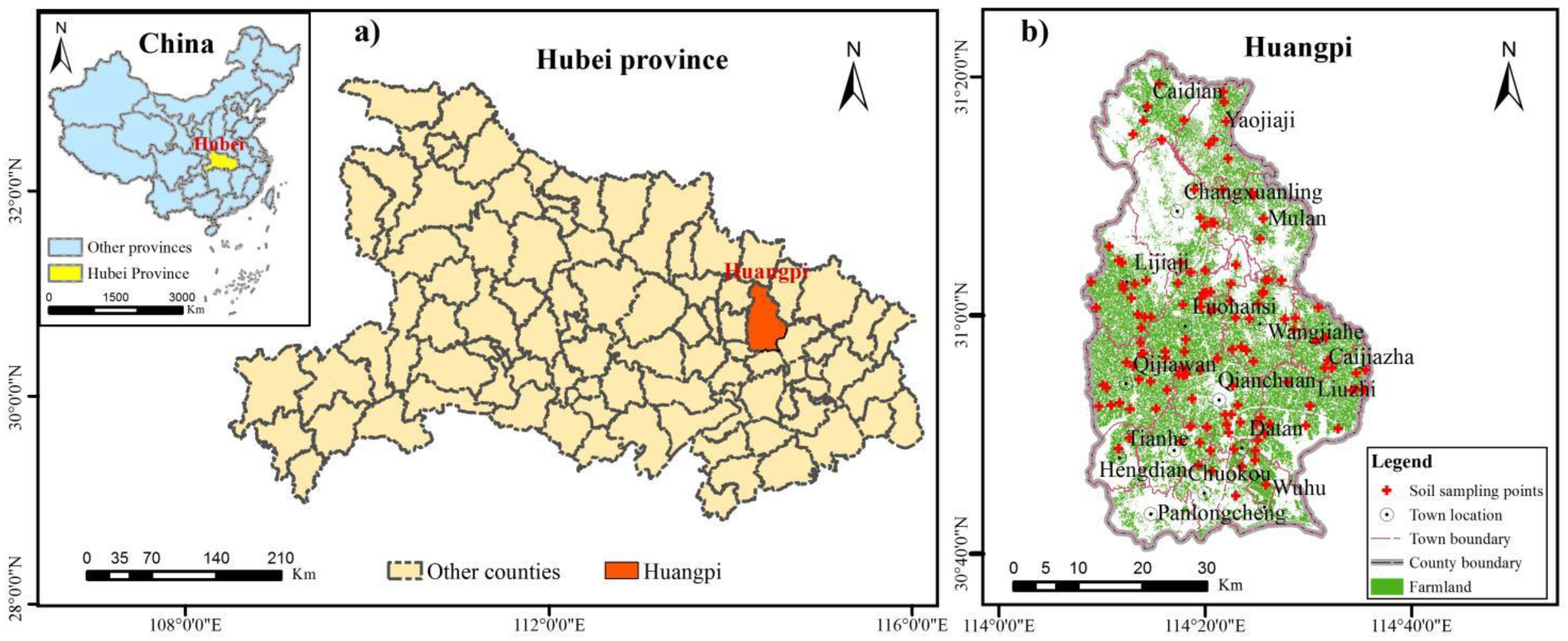
Figure 1. Study area and soil sampling: (a) location in Hubei Province, China; (b) spatial distribution of soil sampling points in Huangpi.
Agriculture 13 00008 g001
Figure 2. Workflow chart.
Agriculture 13 00008 g002
Figure 3. Spectral reflectance data for the same sampling points in different soil types in different periods: (a) fluvo-aquic soils, (b) yellow-brown earths, and (c) paddy soils.
Agriculture 13 00008 g003
Figure 4. Spectral reflectance data for different soil types with different SOM contents in the same period in 2018: (a,d) fluvo-aquic soils; (b,e) yellow-brown earths; (c,f) paddy soils.
Agriculture 13 00008 g004
Figure 5. Importance of the bands of the SOM estimation model for single-temporal images: (a) 20 October 2016; (b) 16 November 2016; (c) 17 October 2018; (d) 16 November 2018; (e) 16 October 2020; (f) 15 November 2020.
Agriculture 13 00008 g005
Figure 6. Scatter plot of the validation set in the RF model based on double-temporal images using the optimal bands and spectral indices as the prediction variables from three years: (a) 2016; (b) 2018; (c) 2020.
Agriculture 13 00008 g006
Figure 7. Distribution of estimated SOM in the plough layer for cultivated land throughout the study area.
Agriculture 13 00008 g007
Table 1. Equations for soil spectral indices computed using single- and multi-temporal images.
Soil Spectral Indices Computed Using Single-Temporal ImagesEquationSoil Spectral Indices Computed Using Multi-Temporal ImagesEquation
D i j S i S j D T m T n _ p i S T m _ ρ i S T n _ ρ i
R i j S i / S j R T m T n _ p i S T m _ p i / S T n _ p i
D T m T n _ p i j S T m _ p i S T n _ p j
N D i j ( S i S j ) / ( S i + S j ) R T m T n _ p i j S T m _ p i / S T n _ p j
Table 2. Statistical description of the SOM (g kg−1) content of the whole, calibration, and validation datasets.
DatasetNumber MinMaxMedian1st Qu a3rd Qu bMeanSDcCV (%) dSKeKUf
Whole dataset13413.7940.6425.5521.5630.0625.865.8422.580.18−0.41
Calibration dataset9413.7940.6425.1420.5528.5625.305.8923.290.43−0.12
Validation dataset4014.2036.6327.2424.2831.1727.185.5620.47−0.45−0.27
Notes: a: First quartile; b: Third quartile; c: Standard deviation; d: Coefficient of variation; e: Skewness; f: Kurtosis.
Table 3. Importance of optimal bands and spectral indices for SOM estimation based on double-temporal images.
YearSingle BandSpectral Indices
2016VariablesB8_1020, B11_1116, B8a_1116, B7_1020, B4_1020, B12_1020, B11_1020D1020-1116_48a, R1020-1116_411, ND1020-1116_411
Importance410.53 328.09, 306.77, 272.36, 256.80, 173.78, 156.6880.30, 61.39, 57.65
2018VariablesB8_1017, B6_1017, B7_1017, B4_1116, B8a_1017, B11_1017, B5_1017D1116-1017_48, D1017-1116_74, D1116-1017_411
Importance444.74, 397.53, 394.66, 337.85, 277.09, 211.02, 195.8463.82, 49.69, 48.22
2020VariablesB11_1016, B8_1115, B7_1016, B4_1016, B5_1016, B8a_1016, B4_1115D1115-1016_84, D1115-1016_47, D1016-1115_48
Importance361.97, 334.69, 333.94, 296.43, 278.03, 226.30, 210.7065.64, 43.06, 41.89
Table 4. Statistical results of the three different modelling algorithms using double-temporal images based on full spectrum data and the optimum bands and spectral indices in 2016, 2018, and 2020.
Modelling StrategiesYearFull SpectrumOptimum Bands and Spectral Indices
CalibrationValidationCalibrationValidation
R2calRMSEcalR2valRMSEvalRPIQvalR2calRMSEcalR2valRMSEvalRPIQval
PLS20160.432.84 0.402.91 2.13 0.542.530.472.892.38
20180.492.55 0.452.74 2.26 0.612.260.532.432.83
20200.472.66 0.442.83 2.19 0.572.460.512.512.74
GWR20160.512.670.482.57 2.42 0.602.270.562.422.85
20180.542.540.502.792.47 0.632.160.592.372.91
20200.522.670.502.762.49 0.612.270.582.352.93
RF20160.592.310.532.392.88 0.652.080.632.153.20
20180.612.10.552.283.02 0.681.890.672.053.36
20200.592.20.542.163.19 0.661.980.642.123.25
Table 5. Statistics for estimates of the SOM content in the plough layer for cultivated land throughout the study area.
Contents/(g kg−1)Area/km2Percentage/%
16.17~22.4796.2810.14
22.47~25.36230.4624.27
25.36~28.12388.5340.91
28.12~32.50147.3115.51
32.50~38.9887.089.17
Disclaimer/Publisher’s Note: The statements, opinions and data contained in all publications are solely those of the individual author(s) and contributor(s) and not of MDPI and/or the editor(s). MDPI and/or the editor(s) disclaim responsibility for any injury to people or property resulting from any ideas, methods, instructions or products referred to in the content.