Abstract
Aboveground biomass (AGB) is an important basis for wheat yield formation. It is useful to timely collect the AGB data to monitor wheat growth and to build high-yielding wheat groups. However, as traditional AGB data acquisition relies on destructive sampling, it is difficult to adapt to the modernization of agriculture, and the estimation accuracy of spectral data alone is low and cannot solve the problem of index saturation at later stages. In this study, an unmanned aerial vehicle (UAV) with an RGB camera and the real-time kinematic (RTK) was used to obtain imagery data and elevation data at the same time during the critical fertility period of wheat. The cumulative percentile and the mean value methods were then used to extract the wheat plant height (PH), and the color indices (CIS) and PH were combined to invert the AGB of wheat using parametric and non-parametric models. The results showed that the accuracy of the model improved with the addition of elevation data, and the model with the highest accuracy of multi-fertility period estimation was PLSR (PH + CIS), with R2, RMSE and NRMSE of 0.81, 1248.48 kg/ha and 21.77%, respectively. Compared to the parametric models, the non-parametric models incorporating PH and CIS greatly improved the prediction of AGB during critical fertility periods in wheat. The inclusion of elevation data therefore greatly improves the accuracy of AGB prediction in wheat compared to traditional spectral prediction models. The fusion of UAV-based elevation data and image information provides a new technical tool for multi-season wheat AGB monitoring.
1. Introduction
Wheat is one of the three major food crops and occupies a dominant position in agricultural production in the world. With the growing population, there has been an increasing demand for wheat in recent years. Therefore, it is essential to improve wheat production efficiency and achieve a high yield for food security and market demand. Aboveground biomass (AGB), a key basis for grain yield formation, plays an important role in light energy utilization [1]. AGB is a crucial indicator of crop response to management practices and environmental conditions [2,3]. Thus, accurate and effective monitoring of wheat biomass at the plot scale can provide strong support for the high-throughput screening of wheat breeding materials [4,5].
Traditional AGB estimation is based on destructive measurement sampling, which is not only labor-intensive and time-consuming, but more seriously, is difficult to apply in large fields [2,6]. Remote sensing is an effective tool for monitoring crop growth season and assessing spatial variability of AGB [6]. In recent years, a large number of studies have been carried out to estimate crop AGB using unmanned aerial vehicles (UAVs) and the main methods can be specifically divided into direct or indirect estimation [7]. The direct method is to build a regression model for AGB estimation based on multiple parameters extracted from the sensors for the measured sample. The common statistical models include parametric and non-parametric models [8]. Parametric models mainly include logistic regression, linear component analysis and perceptual machines. Non-parametric models include decision trees (DT), parsimonious Bayes, support vector machines (SVM) and neural networks (NN). Regular parameters extracted from sensors include color [9], texture [10,11], spectrum [12], etc. The indirect method is to establish the corresponding AGB estimation model based on the response relationship between the agronomic parameters extracted from the UAV images and AGB. The agronomic parameters mainly extracted from UAV images are plant height (PH) [6,13], leaf area [14] and crop canopy cover [15]. Although both modeling approaches for AGB estimation have achieved promising results, the correlation between spectral information and crop AGB varies with the growth period and is closely related to the physiological condition of the crop [6,16]. To solve this problem, it is necessary to conduct field crop monitoring during multiple key growth periods. Biomass estimation of different reproductive periods is a hot topic in the field of remote sensing monitoring. Remote sensing techniques can be used to obtain crop canopy reflectance, and researchers use these spectral features to estimate biomass. However, it was gradually found that spectral features have some limitations in phenotype monitoring and are prone to spectral saturation in late crop reproduction [17]. For such problems, researchers have used synthetic aperture radar (SAR) [18] or incorporated texture features [16], canopy cover [19] and elevation data [13] in the model construction, which reduce the reliance of the model on spectral data. It has been demonstrated that the inclusion of elevation data has a significant positive effect on the improvement of biomass estimation accuracy.
Crop PH is an important indicator reflecting the crop growth status. Researchers have shown the correlation between PH and crop biomass [14,20]. With the development of remote sensing technology, the extraction methods of PH are gradually enriched. The measured height is a common approach used to assess crop height. The calculation of crop height measurement based on UAV is obtained by extracting the crop surface model (CSM). CSM refers to the difference between a digital surface model (DSM) (the altitude of the vegetation on top of the bare soil) and the corresponding digital elevation model (DEM) (the altitude of the bare soil) [14]. LiDAR, ultrasonic, depth cameras and other sensors can directly obtain elevation information, but such sensors also have some defects and are not conducive to the actual production and application. For instance, LiDAR obtains elevation information by laser time of flight, has strong penetration and works independently of ambient light, but is difficult to apply in practice due to its high cost and difficult data processing [20]. Ultrasound has been used in agriculture for a long time and works on a similar principle to LiDAR, emitting ultrasonic pulses as a measure of detecting information about an object. However, ultrasonic signals are susceptible to the environment and distance, and ultrasound can only detect objects at close range, which limits the application scenarios of this sensor and the need to meet the growing demand for high-throughput phenotype monitoring [21,22]. The depth cameras suffer from similar problems to the ultrasonic sensor. Compared to the sensors mentioned above, the use of UAVs with RGB cameras is less costly. The UAV measurement applies the structure from motion (SfM) technique for feature detection and matching of captured images to construct a point cloud model, which is combined with interpolation to generate elevation data [23].
As an emerging remote sensing platform, UAVs, with their low cost, high efficiency and flexibility, can make up for the inability of satellite remote sensing to acquire data due to factors such as transit time and environment [24]. Rapid advances in UAV technology have made it increasingly easy to acquire remote sensing data at the ultra-high spatial resolution [25,26], and UAVs can carry multiple sensors (e.g., RGB, multispectral and LiDAR) for the task of collecting remote sensing information from multiple sources in a single flight [27]. The physiological parameters estimated based on radar 3D point cloud data are less susceptible to saturation issues with high-density vegetation [20,28,29]. The SfM enables the reconstruction of 3D point clouds from high-resolution RGB images, which provides a new, more cost-effective technique for the acquisition of point cloud data [30,31]. The 3D point clouds reconstructed from RGB images have been successfully used to extract the canopy structure of vegetation and to estimate physiological parameters such as crop height and biomass [30,31,32]. For example, Geipel et al. [33] found that combining vegetation indices (VIs) with PH could improve the accuracy of maize yield prediction. Qin et al. [34] proposed that the fusion of hyperspectral data and LiDAR measurements of PH significantly improved the accuracy of maize fAPAR estimation. Maimaitijiang et al. [35] and Wan et al. [23] found that the combination of spectral and structural information based on UAVs was effective in estimating soybean and rice yields, and that the fusion data improved the ability to monitor aspects of crop growth conditions.
Although an increasing number of researchers have reported that combining spectral data with SfM-based structural features from UAV data can improve the robustness of predicting crop AGB, as structural features help to mitigate canopy spectral saturation [10,24,36,37], some uncertainties remain. Mao et al. [38] demonstrated that the combination of spectral and structural features did not improve the accuracy of biomass estimation in desert shrubs. Bendig et al. [39] found that the combination of visible light band characteristics and PH had little impact on the biomass estimation of barley. Therefore, it is unclear whether the combination of RGB color indices (CIS) with structural features can improve the AGB estimation in wheat, because canopy structure and AGB composition changes dynamically throughout the growth cycle. In addition, the density of the plants and the size of the crop canopy vary across the period of growth and the different field treatments [40]. Although the UAVs are able to obtain elevation information, the canopy height does not change significantly in the later stages of fertility, and the PH measured using the camera technique is not acceptable for estimating the canopy of high-density crops. Therefore, it is not feasible to estimate wheat biomass based only on the average PH at a single scale (throughout the growing season). Based on this issue, this paper used two PH calculation methods (mean values and cumulative height percentile methods) to extract wheat PH, which were combined with RGB CIS, and estimated the wheat AGB using parametric and non-parametric models at multiple stages. Therefore, the main objectives of this study were to (1) quantify the utility of color and structural features (PH) in estimating wheat AGB variability across multiple periods, (2) assess whether combining canopy color and structural features could improve wheat AGB estimation across treatments.
2. Materials and Methods
2.1. Experimental Design
The trials of winter wheat were conducted for two growing seasons (2019–2020, 2020–2021) at the experimental fields of Fengling Reservoir, Yizheng City, Yangzhou City, Jiangsu Province (32°16′ N, 119°12′ E). The test areas were located in the middle and lower reaches of the Yangtze River plain, which belong to the north subtropical monsoon climate, with an annual average temperature of about 15 °C and annual precipitation of about 1200 mm. The soil type of the test field was loamy with a hydrolytic N content of 87.22 mg/g, an effective phosphorus content of 30.16 mg/g and an effective potassium content of 121.35 mg/g in the top 20 cm soil layer.
Three variables were considered in the two-year field experiment, including different varieties, planting densities and N application rates (Table 1). The trial was conducted in a randomized group trial designed with three replications, including three varieties (Zhenmai 12, Yangmai 16 and Ningmai 13), three planting densities (M1: 1.5 million plant/ha, M2: 2.25 million plant/ha and M3: 3 million plant/ha) and four N application levels (N0: 0 kg/ha, N1: 125 kg/ha, N2: 225 kg/ha and N3: 375 kg/ha). A total of 216 plots (each plot 3 m × 4 m, or 12 m2) were used in the two-year trial. Urea was applied at the ratio of 5:1:2:2 as basal fertilizer, tiller fertilizer, nodulation fertilizer and ears fertilizer. Approximately 120 kg/ha of phosphorus and potassium fertilizer were split as basal fertilizer and nodulation fertilizer. The details of the experiment can be seen in Table 1. Other field management practices followed the actual production of winter wheat in local fields.

Table 1.
Information on the field experiments.
Eighteen ground control points (GCPs) were placed in the test area for the correction of elevation data, and the test plot layout is shown in Figure 1. The specifications of ground control points were 0.8, 1 and 1.2 m, with a total of 6 GCPs for each specification. One GCP was placed between every two plots in a gradient pattern. The spatial position information of these GCPs was positioned using Global Navigation Satellite System (GNSS) receivers carried on the UAV and calibrated for measurement using the built-in real-time kinematic (RTK). At the same time, the actual GCP heights were measured manually before each flight shooting for later calibration.
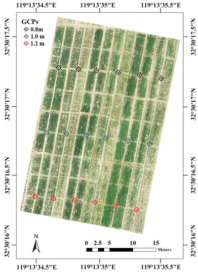
Figure 1.
Wheat experiments conducted at the Yizheng Experimental Station in Jiangsu Province, China.
2.2. Data Acquisition
2.2.1. UAV Image Acquisition and Pre-Processing
In this study, a DJI Phantom 4 RTK UAV (SZ DJI Technology, Co., Shenzhen, China) was used for field image data acquisition. RGB images were acquired for bare soil before sowing and for vegetation during different periods such as jointing, booting and flowering stages. The DJI Phantom 4 RTK UAV is a small, lightweight, easy-to-carry, multi-rotor and high-precision aerial survey drone equipped with centimeter-level navigation and positioning system and a high-performance imaging system. The drone was equipped with an RGB camera with 20 megapixel CMOS and a 24 mm focal length sensor. The built-in RTK and GNSS give it precise positioning capabilities that can significantly improve the absolute accuracy of image metadata. Prior to image acquisition, 18 GCPs (Figure 1) were set up uniformly throughout the study plots, and the spatial position information of these GCPs was positioned using GNSS receivers and calibrated for measurement using RTK with a horizontal error of 0.01 m and a vertical error of 0.015 m. All flight missions were performed from 10:30 a.m. to 14:00 p.m. under cloud-free days with low wind. The flight altitude was 25 m, the image repetition rate was set to 70%, and the resolution of the aerial images was 0.8 × 0.8 cm.
After RGB image acquisition, the photogrammetric software, Pix4Dmapper (Pix4D SA, Lausanne, Switzerland), was used to generate 3D point cloud data and a DSM. In the software, images were aligned according to the tie points, and then geometrically corrected and mosaicked to generate high-density point clouds. For the aim of building accurate and high-density point clouds, the “original image size” and “high” options were selected in the point cloud settings, then these point clouds were georeferenced by merging the geographic coordinates of 18 GCPs. Subsequently, mesh and texture were constructed based on the generated point clouds, resulting in a DSM and a digital orthophoto map (DOM). In addition, the bare soil images were processed using the above method and the resulting digital elevation model was noted as a DEM, as shown in Figure 2.
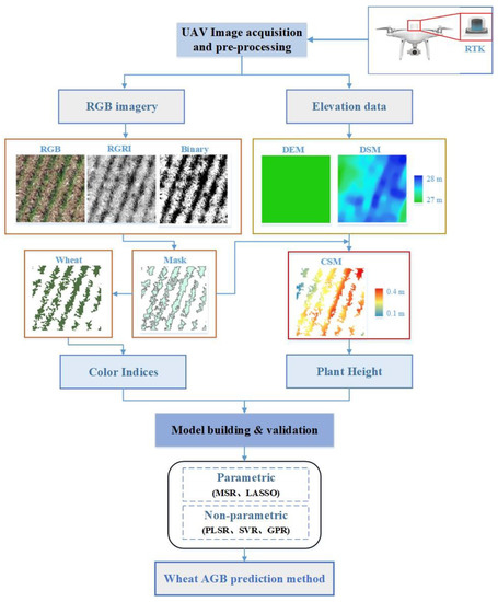
Figure 2.
The main process of this study.
2.2.2. Field Data Collection
A ground sampling of winter wheat was carried out after the imagery collection. Twenty wheat plants were randomly selected from the sampling sites at the jointing, booting and flowering stages, and PHs were measured with a ruler, followed by destructive sampling. Plant samples were separated into different organs in the laboratory, including leaves, stalks and spikes. After drying in an oven at 80 °C to a constant weight, the dry weights of the plant organs were then weighed. The AGB for each period was then determined from the sum of the dry weights of the organs. There were 648 plant samples collected over two years from three growth stages.
2.3. CIS and PH
2.3.1. Extraction of CIS
UAV RGB images were spatial images with three color components, red, green and blue. The color indices calculated by the three components have a significant correlation with the dynamic change in crop growth. Based on the results of previous studies on predicting biomass, 17 of the more widely used CIS (Table 2) were selected for AGB estimation in this study. Prior to the extraction of CIS, background soil was removed from the raster layer of RGB images by calculating the RGRI (red-green ratio index) parameter using Band Math in ENVI 5.3 software (Exelis Visual Information Solutions, Boulder, CO, USA), to classify plants and others. Then, the classification was used to generate a binary mask layer to extract CIS. The digital number (DN) for the red, green, and blue bands of the extracted wheat layers were expressed as R, G and B, respectively. The normalizations of the three colors components were calculated by the following formula:
Table 2.
CIS used in this study.
2.3.2. Calculation of PH
PH is a useful indicator of plant growth. Pix4Dmapper software (Pix4D SA, Lausanne, Switzerland) was used to generate DSM and DOM for each flight. The CSM is widely applied for different crops to extract PH, which is the difference between the DSM and the DEM. In this study, two commonly used CSM calculation methods, namely the mean value method [16] and the cumulative percentile method [50,51], were conducted to obtain PH at different stages of winter wheat.
The binary mask layer generated from the RGRI index was stacked with the elevation images (DSM) to remove the confounding image elements and to extract the vegetation elevation information. Using zonal statistics, the mean value method was used to extract the mean PH of each plot from the CSM. Plant heights were validated by one-third of the total sample (n = 648) measured at the plot level.
The cumulative percentile method involved importing the DSM into ENVI 5.3 software and calculating the percentile pixel values for each plot from 90 to 100% in a 0.5 percentile interval, with the different percentile pixel values corresponding to different undulating plant heights. To achieve the optimal PH, the lower percentile height value was considered as the base boundary and the higher percentile height value (90–100%) as the upper plant boundary. Finally, the height of the base plant boundary was subtracted from the height of the upper boundary at different percentiles to calculate the estimated PH for each plot.
2.4. Modeling Methods: Parametric and Non-Parametric Models
Two different statistical models, including parametric (multiple stepwise regression (MSR), least absolute shrinkage and selection operator (LASSO)) and non-parametric (partial least square (PLSR), support vector regression (SVR) and Gaussian process regression (GPR)), were analyzed in this study in order to assess the improvement in the accuracy of AGB estimation for wheat at multiple developmental stages by the combination of CIS and PH.
2.4.1. Parametric Models
In past studies, empirical models based on parametric regression have been widely used for AGB estimation in agricultural contexts. Parametric models assume a direct relationship between color features and biomass to establish parametric statistical relationships [52]. The parametric models in this study included MSR and LASSO, which were chosen to explore the statistical relationships between CIS, PH variables and AGB.
MSR is generally used to investigate the linear relationship between a dependent variable and multiple independent variables [53]. This paper used a stepwise method to screen the independent variables. The stepwise method performs an F-test for each new independent variable introduced, and subsequently recalculates the already substituted independent variables, re-evaluates their values within the equation using a T-test, and then decides to retain or eliminate them, alternating the cycle until no new variables can be introduced or eliminated, thus obtaining the optimal model.
First proposed by Tibshirani [54] in 1996, LASSO regression is a compression estimation method based on the principle of reducing the set of variables. By constructing a penalty function, the coefficients of variables are compressed to achieve the purpose of variable selection. LASSO performs well on the problem of large overfitting in linear regression by introducing regularization in the loss function.
2.4.2. Non-Parametric Models
Non-parametric models are data-driven modeling approaches derived from the direct definition of regression models based on information from given remote sensing data and relevant variables [52]. In this study, three different non-parametric models, including PLSR, SVR and GPR, were analyzed to evaluate the improvement of wheat biomass estimation accuracy by the combinations of color and PH at different growth stages.
PLSR is an integration of principal component analysis and typical correlation analysis on the basis of linear regression [55]. PLSR was initially used for regression relationships between multiple independent variables and multiple dependent variables, but in later studies it was also commonly used for regression analysis between single dependent variables and multiple independent variables [56,57]. PLSR eliminates possible multi-collinearity among variables and makes that regression analysis performed under conditions of multiple correlations and with a smaller sample size than the number of variables. Therefore, PLSR is more explanatory.
Support vector machine is one of the machine learning algorithms that can be used for classification and regression [58,59,60]. In this paper, SVR was selected and used to map the data linearly or nonlinearly through the selection of kernel functions, so as to map the data into a high-dimensional space and construct the optimal regression function in the high-dimensional space. The SVR method has advantages in solving problems such as small samples and co-linearity.
GPR is a non-parametric model that belongs to a kernel-based approach and relies on solid Bayesian formalism, thus allowing for a formal treatment of uncertainty quantification and error propagation [61,62,63]. Regression analysis of data using GPR leads to the construction of models based on generalizability, which is often used for solving problems having few sample data.
2.5. Wheat AGB Modeling and Validation
Two-thirds of the total sample size was used as the training set (n = 432) and one-third as the validation set (n = 216) to construct wheat biomass estimation models for single and multi-fertility periods, respectively. The calibration dataset was used to adjust the model parameters, while the validation dataset was used to confirm the true predictive ability of the model built and had no impact on the model construction [40].
In this study, the coefficient of determination (R2), root mean square error (RMSE) and normalized root mean square error (NRMSE) were used to assess the accuracy of wheat AGB predicted by different models, and the three indicators were calculated as follows:
where xi is the measured value of sample i, yi is the estimated value of sample i, x is the mean of the measured values of the sample and n is the total number of samples.
3. Results
3.1. Statistical Analysis of PH and AGB
Table 3 shows the statistical results for measured PH and biomass. The coefficient of variation for PH in Exp. 1 was greater than 10% for all periods and showed a gradual decrease, while the coefficient of variation for biomass was greater than 20% for all periods, with the coefficient of variation varying more before than after tasseling. The analysis of the Exp. 2 data set was consistent with these results. Overall, the two-year wheat experiment provided a suitable dataset with large variability for optimizing the wheat AGB monitoring model using PH.
Table 3.
Descriptive statistics for PH and AGB from Exp. 1 and Exp. 2 datasets across wheat growth stages.
3.2. PH Estimation
Wheat PH values were extracted using the cumulative percentile method and the mean method, respectively. As can be seen from Figure 3, the R2, RMSE and NRMSE of PH extracted from the 90th to 100th percentile and the measured PH showed good accuracy at the jointing, booting and flowering stages. Meanwhile, R2 showed a pattern of increasing and then decreasing values with the rising percentile during all three periods, and RMSE and NRMSE showed a pattern of decreasing and then increasing in general. However, owing to the small division interval, the changes in R2, RMSE and NRMSE were flatter. The three indicators of PH extracted at the 100th percentile were lower than those at the 98th to 99.5th percentile.
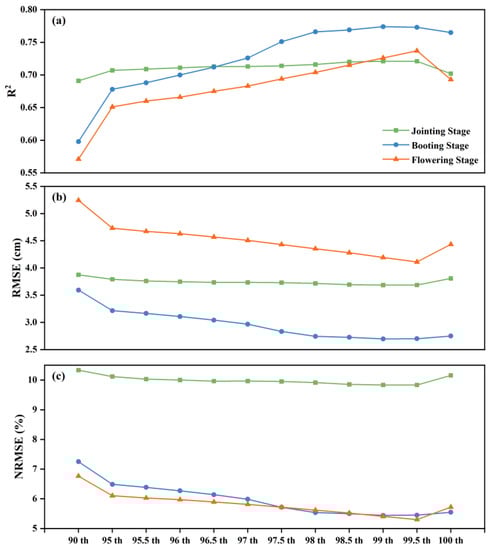
Figure 3.
Results of the plant height estimation based on elevation data using the cumulative percentile method. Note: (a) coefficient of determination, (b) root mean square error, (c) normalized root mean square error.
The constructed model for estimating wheat PH was validated using data from the validation set (Figure 4). In this paper, the actual and estimated values of PH fitted well at different developmental stages. The cumulative percentile method was more accurate than the mean method for monitoring the height of wheat plants during all three fertility periods. Therefore, for the later estimation of biomass, the fused PH data was calculated using a model constructed by the cumulative percentile method.
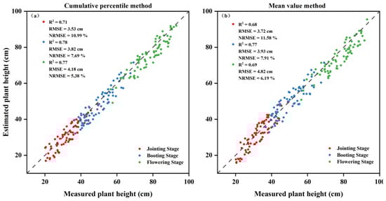
Figure 4.
Relationship between measured and estimated plant height (cm) using the (a) cumulative percentile method and the (b) mean value method.
3.3. AGB Estimation
3.3.1. Correlation between CIS and AGB
Correlation coefficients (r) were determined between the AGB and CIS. As shown in Figure 5, the 12 CIS: ExG, MGRVI, NDI, ExGR, RGBVI, GRRI, RGRI, BGRI, NGBDI, GIVE, VEG and COM, were correlated with AGB in all three stages at highly significant levels. The correlations of VARI, BRRI, NPCI, IF and WI with biomass at all stages of wheat had different levels of correlation. The color index, VARI, did not reach significant levels only at the jointing stage, but the correlation between VARI and biomass reached significant levels at the booting and flowering stages. BRRI and NPCI were only correlated to highly significant levels with biomass at the jointing stage, while IF and WI were correlated to highly significant levels in jointing stage and flowering stage except for biomass at the booting stage. In addition, BGRI, GIVE, GRRI and VEG showed the best correlations at jointing, booting and flowering with their correlation coefficients of −0.795, −0.855 and 0.898, respectively.
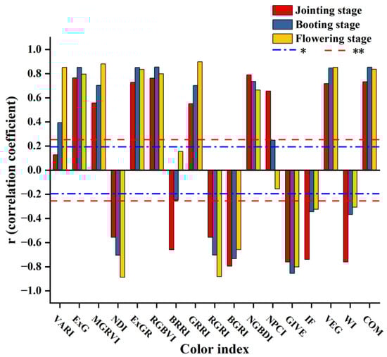
Figure 5.
Correlation coefficient (r) between CIS and AGB. Note: * indicates significance at p < 0.05, and ** indicates significance at p < 0.01.
3.3.2. Use of CIS to Estimate AGB
Figure 6 showed the modeling effect of the single color index to estimate biomass. As the reproductive period advanced, the estimated accuracy showed an increasing trend. The PLSR method had the highest estimation accuracy with R2 of 0.68 and 0.77, RMSE of 374 kg/ha and 830.12 kg/ha, and NRMSE of 15.23% and 15.57% at the jointing and booting stages, respectively. The best estimation method for flowering and multi-stages was LASSO with R2 of 0.85 and 0.73, RMSE of 963 kg/ha and 1485.04 kg/ha, and NRMSE of 12.58% and 27.74%, respectively. In general, the prediction accuracy of all five models based on the CIS should be improved.
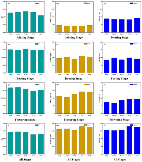
Figure 6.
Results of the AGB estimation based on CIS at (a–c) jointing stage, (d–f) booting stage, (g–i) flowering stage, (j–l) all stages.
3.3.3. Use of CIS and PH to Estimate AGB
The results of the AGB estimation by combining the PH with the CIS are shown in Figure 7. The estimation accuracy of the models was significantly improved by integrating the PH data, and the accuracy of all models was higher than 0.7, except for the jointing stage. Overall, among the three reproductive periods, the estimation accuracy of PLSR was the best, with the highest R2 of 0.9, RMSE of 831.86 kg/ha, and NRMSE of 11.50%. The accuracy of the PLSR method was the most stable and least influenced by the periods.
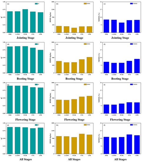
Figure 7.
Results of the AGB estimation based on CIS + PH at (a–c) jointing stage, (d–f) booting stage, (g–i) flowering stage, (j–l) all stages.
3.4. Evaluation of Model Prediction Accuracy
As shown in Figure 8, the predicted and measured values of wheat AGB showed good agreement, especially with the advancement of the fertility period, and the prediction accuracy of the model became higher. For the wheat AGB prediction models at the jointing stage, the R2 values of the regression models constructed based on CIS and on the combination of CIS and PH were MSR (0.63 and 0.73), LASSO (0.42 and 0.57), PLSR (0.42 and 0.57), SVR (0.51 and 0.56) and GPR (0.59 and 0.63), respectively, with the constructed MSR method having the highest accuracy for the model. The R2 values of the CIS-based and CIS + PH-based booting AGB estimation models constructed by the five algorithms were MSR (0.69 and 0.81), LASSO (0.69 and 0.84), PLSR (0.68 and 0.81), SVR (0.68 and 0.79) and GPR (0.52 and 0.73), respectively. The LASSO model for the booting stage had the highest accuracy and the most significant improvement in the prediction accuracy of the model with the incorporation of PH. The R2 values of the CIS-based and CIS + PH-based flowering AGB estimation models constructed by the five algorithms were MSR (0.73 and 0.81), LASSO (0.73 and 0.81), PLSR (0.74 and 0.83), SVR (0.75 and 0.83) and GPR (0.73 and 0.79), respectively, with the model constructed by the PLSR method having the highest accuracy. Compared with the model prediction accuracy of single fertility, the difference among the model prediction accuracies of the five methods for multiple fertility periods was small and more stable.
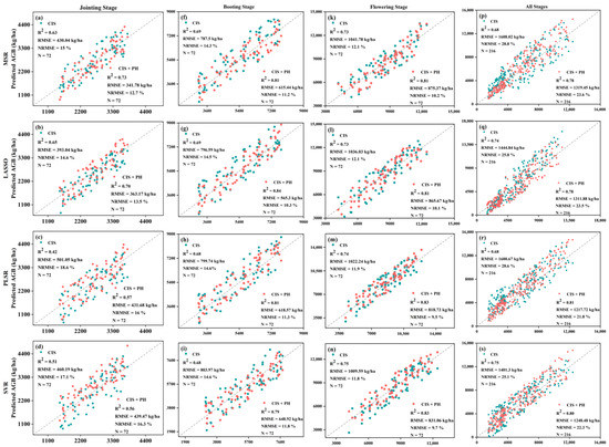
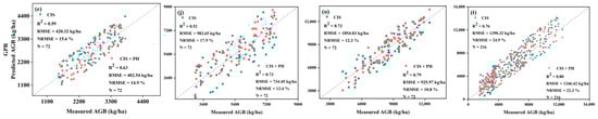
Figure 8.
Relationships between the measured and the predicted AGB (kg/ha) based on CIS or CIS + PH using five regression models at different stages. Note: (a–e) jointing stage, (f–j) booting stage, (k–o) flowering stage, (p–t) all stages.
4. Discussion
4.1. Inversion of PH
Many studies have been carried out on the extraction of PH as an important indicator of the growth status of crops. Liu et al. [64] evaluated the validity of point clouds obtained from UAV-based LiDAR to estimate the mean height of trees. Ziliani et al. [65] and Grüner et al. [66] successfully extracted crop height using a UAV carrying a high-resolution RGB camera. Although the methods of PH estimation have been studied in the past, there are few comparative studies on the accuracy of these methods. In this study, two commonly used methods for estimating PH were analyzed and the optimal model for each period of wheat and the optimal method for both estimation methods were derived by comparing them using three indicators, R2, RMSE and NRMSE. The results showed that the accuracy of the cumulative height percentile method was better than that of the mean value method, but the difference between the two methods was small. The reason for this was mainly from the grasp of the canopy height [67]. The mean value method uses CSM to directly average the elevation difference between DSM and DEM as the PH of crops. However, the disadvantage of this method may be that if the plant type is loose or the planting density is low, some parts below the canopy will also be recorded as the PH, thus reducing the extracted PH. We found this problem during the pre-processing of the data. Therefore, when processing the images at low planting densities, we dispersed the ROI at the canopy to avoid taking the lower part of the plant, while ensuring that the same image DN values were selected as in the high-planting-density plots. As the result, the extracted heights of the plants did not show significant differences at different density conditions in this study. This also demonstrates the broader applicability of the method in this study. The cumulative height percentile method uses the height value of the high percentile as the upper boundary, which can avoid the influence of the lower blade. In addition, the PH extraction based on the cumulative height percentile method, with the increase in the high percentile, the overall PH extraction accuracy showed a trend of first rising and then declining, and generally started to decline at the 100th percentile, reaching the best at the 99th or 99.5th percentile. The experimental results were consistent with those of Madec et al. [20] and differed from Lu et al. [50] and Niu et al. [51]. The main reason for this discrepancy may be that the subject of this study was wheat, where the canopy tip consists of grain heads. In contrast, the subject of the other two studies was maize, where the canopy top was a tassel and the distribution of point clouds at the top of maize was sparser than wheat.
4.2. Evaluation of Model Estimation Performance by Extracted PH
The changes in the modeling accuracy of the CIS-based AGB estimation models were compared with that of the CIS + PH-based estimation models, and histograms (Figure 9) were created for further analysis. As shown in Figure 9, the amount of R2 variation was positive and the RMSE and NRMSE were negative at all fertility stages, indicating that the addition of extracted PH improved the fit of different estimation models for wheat biomass at different fertility stages, reduced the estimation error and improved the estimation accuracy.
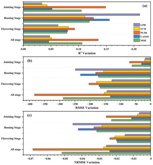
Figure 9.
Comparison of (a) R2 variation, (b) RMSE variation and (c) NRMSE variation between estimation model with CIS and estimation model with CIS + PH.
Analysis of the effect of PH on the coefficient of determination for the models showed that PH had the greatest effect on the accuracy of the multi-fertility estimation models, and that the multi-fertility estimation models improved more than the single-period models. The non-parametric models outperformed the parametric models during the jointing period, except for SVR, which had a lower R2 variation than the two parametric models, with the GPR model showing the greatest improvement. At the booting stage, all models, especially the GPR model, showed a high increase with the addition of the PH parameter. In the estimation models for flowering and multi-fertility, the non-parametric models showed greater improvement than the parametric models, with the SVR showing the greatest improvement. In the construction of the biomass estimation model with CIS + PH, it was found that the modeling accuracy of the non-parametric model was generally higher than that of the parametric model at the jointing stage and lower than that of the parametric model at the booting stage, while the validation accuracy of the non-parametric model was lower than that of the parametric model at both fertility stages (jointing and booting). Both types of models (parametric and non-parametric) had high accuracy and little difference in estimation at flowering. The non-parametric models had higher estimation accuracy and stability than the parametric models over multiple periods. Thus, the addition of PH had a positive effect on the biomass estimates of all models during all fertility periods. In comparison, the non-parametric models showed the highest overall enhancement, and both parametric and non-parametric models responded most strongly to PH during multiple fertility periods.
According to our research, the extracted PH information is valid for biomass estimation at the jointing, booting, flowering and multi-fertility stages. The extracted PH improved the AGB estimation models for different fertility stages, probably because PH was an important indicator of wheat growth and development, and the dynamic change in PH indicated to some extent the ability of wheat source–sink organ development, reflecting the positive growth of wheat [51]. Secondly, multivariate traits inherently incorporate spatial and temporal variation in wheat populations and are consistently better predictors of biomass than single variables [68,69,70]. Previous studies have also reported that different canopy height estimates can improve the accuracy of biomass prediction [71,72].
4.3. Comparison of Modeling Methods
Parametric and non-parametric models are two types of models based on empirical models. In this paper, a few representative modeling methods were selected for comparing the differences between the two types of models. By comparing the CIS-based and the accuracy of the model after the addition of PH, it was found that the parametric models were more stable than the non-parametric models both before and after the addition of PH. This is consistent with the findings of Zheng et al. [73], which is mainly because non-parametric models have certain requirements for sample size and feature parameters, and failure to meet the requirements results in a decrease in validation accuracy. In multi-fertility modeling, the stability and accuracy of the non-parametric model with the addition of PH were greatly improved compared to the previous one, indicating that the addition of PH greatly improved the model performance. The reason for this is that the combination of the CIS is relatively simple, with the potential for covariance problems and easy overfitting in non-parametric models, whereas PH, as a morphological index with a highly significant relationship to biomass, can well compensate for the lack of CIS. At the same time, adding PH to the model can reduce the dependence of the model on CIS and effectively solve the problem of CIS saturation in the later stage of growth, thus improving accuracy.
Niu et al. [51] suggested that simple linear regression performed better with a small range of PH, while empirical models usually performed better with a large range of PH. This finding was consistent with the present study, where the range of variation in PH under multi-fertility was large and both the single and multi-fertility AGB estimation models fused by PH and CIS performed better as non-parametric models. The MSR model performed poorly in the use of CIS, with most of the estimation models for each fertility period only being able to utilize one color index for modeling, which also existed in a previous study [19,74,75]. In contrast, LASSO was chosen less in previous biomass estimation studies, but as a model capable of compressing coefficients and solving the co-linearity problem [76,77], the results showed that the overall estimation was better than that for the MSR model, while also adopting more CIS and better tapping into the class of variables consisting of simple information such as CIS. Therefore, in future research, the use of the LASSO regression model can be gradually increased and deepened to improve the value of the model in the field of agricultural remote sensing monitoring.
5. Conclusions
In this study, the crop surface model and high-resolution digital canopy image of wheat were obtained by a high-precision UAV carrying RTK, and the PH data of wheat were successfully extracted, and then the wheat AGB estimation models were constructed based on CIS and after adding PH. It was concluded that the PH estimation method based on the CIS estimation method had the lowest accuracy, and the PH extraction method based on the cumulative height percentile method was consistently more accurate than the mean value method at all fertility stages, compared to the two types of PH extraction methods based on elevation data. Therefore, this study concluded that the PH extraction method based on the cumulative height percentile method is more suitable for UAVs. In the process of constructing the wheat AGB estimation model, the accuracy of the AGB estimation model was significantly improved by adding PH data to both parametric and non-parametric models. Through the analysis of results, the non-parametric model is more susceptible to the influence of PH parameters, and the PLSR (CIS + PH) model has high accuracy and stability.
Author Contributions
Conceptualization, W.G., D.W. and R.L.; methodology, D.W.; data curation, B.Z.; formal analysis, D.W.; investigation, R.L., T.L. and C.S.; resources, B.Z.; writing—original draft, R.L. and D.W.; writing—review and editing, B.Z. All authors have read and agreed to the published version of the manuscript.
Funding
This research was funded by the National Natural Science Foundation of China (31701355, 31872852 and 32172111); the National Key Research and Development Program of China (2018YFD0300805); and the Postgraduate Research and Practice Innovation Program of Jiangsu Province (XKYCX19_105).
Institutional Review Board Statement
Not applicable.
Data Availability Statement
Not applicable.
Acknowledgments
The authors wish to thank all those who helped in this research.
Conflicts of Interest
The authors declare no conflict of interest.
References
- Jin, X.; Madec, S.; Dutartre, D.; de Solan, B.; Comar, A.; Baret, F. High-Throughput Measurements of Stem Characteristics to Estimate Ear Density and Above-Ground Biomass. Plant Phenomics 2019, 2019, 4820305. [Google Scholar] [CrossRef] [PubMed]
- Yue, J.; Feng, H.; Yang, G.; Li, Z. A Comparison of Regression Techniques for Estimation of Above-Ground Winter Wheat Biomass Using Near-Surface Spectroscopy. Remote Sens. 2018, 10, 66. [Google Scholar] [CrossRef]
- Araus, J.L.; Cairns, J.E. Field High-Throughput Phenotyping: The New Crop Breeding Frontier. Trends Plant Sci. 2014, 19, 52–61. [Google Scholar] [CrossRef] [PubMed]
- Chen, Q.; He, A.; Wang, W.; Peng, S.; Huang, J.; Cui, K.; Nie, L. Comparisons of Regeneration Rate and Yields Performance between Inbred and Hybrid Rice Cultivars in a Direct Seeding Rice-Ratoon Rice System in Central China. Field Crops Res. 2018, 223, 164–170. [Google Scholar] [CrossRef]
- Dong, H.; Chen, Q.; Wang, W.; Peng, S.; Huang, J.; Cui, K.; Nie, L. The Growth and Yield of a Wet-Seeded Rice-Ratoon Rice System in Central China. Field Crops Res. 2017, 208, 55–59. [Google Scholar] [CrossRef]
- Li, B.; Xu, X.; Zhang, L.; Han, J.; Bian, C.; Li, G.; Liu, J.; Jin, L. Above-Ground Biomass Estimation and Yield Prediction in Potato by Using UAV-Based RGB and Hyperspectral Imaging. ISPRS J. Photogramm. Remote Sens. 2020, 162, 161–172. [Google Scholar] [CrossRef]
- Bossung, C.; Schlerf, M.; Machwitz, M. Estimation of Canopy Nitrogen Content in Winter Wheat from Sentinel-2 Images for Operational Agricultural Monitoring. Precis. Agric. 2022, 23, 2229–2252. [Google Scholar] [CrossRef]
- Brewka, G. Artificial Intelligence—A Modern Approach by Stuart Russell and Peter Norvig, Prentice Hall. Series in Artificial Intelligence, Englewood Cliffs, NJ. Knowl. Eng. Rev. 1996, 11, 78–79. [Google Scholar] [CrossRef]
- Yue, J.; Yang, G.; Tian, Q.; Feng, H.; Xu, K.; Zhou, C. Estimate of Winter-Wheat above-Ground Biomass Based on UAV Ultrahigh-Ground-Resolution Image Textures and Vegetation Indices. ISPRS J. Photogramm. Remote Sens. 2019, 150, 226–244. [Google Scholar] [CrossRef]
- Li, W.; Niu, Z.; Chen, H.; Li, D.; Wu, M.; Zhao, W. Remote Estimation of Canopy Height and Aboveground Biomass of Maize Using High-Resolution Stereo Images from a Low-Cost Unmanned Aerial Vehicle System. Ecol. Indic. 2016, 67, 637–648. [Google Scholar] [CrossRef]
- Zheng, H.; Cheng, T.; Zhou, M.; Li, D.; Yao, X.; Tian, Y.; Cao, W.; Zhu, Y. Improved Estimation of Rice Aboveground Biomass Combining Textural and Spectral Analysis of UAV Imagery. Precis. Agric. 2019, 20, 611–629. [Google Scholar] [CrossRef]
- Jiang, Q.; Fang, S.; Peng, Y.; Gong, Y.; Zhu, R.; Wu, X.; Ma, Y.; Duan, B.; Liu, J. UAV-Based Biomass Estimation for Rice-Combining Spectral, TIN-Based Structural and Meteorological Features. Remote Sens. 2019, 11, 890. [Google Scholar] [CrossRef]
- Tilly, N.; Aasen, H.; Bareth, G. Fusion of Plant Height and Vegetation Indices for the Estimation of Barley Biomass. Remote Sens. 2015, 7, 11449–11480. [Google Scholar] [CrossRef]
- Lu, W.; Okayama, T.; Komatsuzaki, M. Rice Height Monitoring between Different Estimation Models Using UAV Photogrammetry and Multispectral Technology. Remote Sens. 2022, 14, 78. [Google Scholar] [CrossRef]
- Yan, G.; Li, L.; Coy, A.; Mu, X.; Chen, S.; Xie, D.; Zhang, W.; Shen, Q.; Zhou, H. Improving the Estimation of Fractional Vegetation Cover from UAV RGB Imagery by Colour Unmixing. ISPRS J. Photogramm. Remote Sens. 2019, 158, 23–34. [Google Scholar] [CrossRef]
- Xu, L.; Zhou, L.; Meng, R.; Zhao, F.; Lv, Z.; Xu, B.; Zeng, L.; Yu, X.; Peng, S. An Improved Approach to Estimate Ratoon Rice Aboveground Biomass by Integrating UAV-Based Spectral, Textural and Structural Features. Precis. Agric. 2022, 23, 1276–1301. [Google Scholar] [CrossRef]
- Fu, Y.; Yang, G.; Wang, J.; Song, X.; Feng, H. Winter Wheat Biomass Estimation Based on Spectral Indices, Band Depth Analysis and Partial Least Squares Regression Using Hyperspectral Measurements. Comput. Electron. Agric. 2014, 100, 51–59. [Google Scholar] [CrossRef]
- Li, S.; Potter, C. Patterns of Aboveground Biomass Regeneration in Post-Fire Coastal Scrub Communities. GISci. Remote Sens. 2012, 49, 182–201. [Google Scholar] [CrossRef]
- Lee, K.-J.; Lee, B.-W. Estimation of Rice Growth and Nitrogen Nutrition Status Using Color Digital Camera Image Analysis. Eur. J. Agron. 2013, 48, 57–65. [Google Scholar] [CrossRef]
- Madec, S.; Baret, F.; de Solan, B.; Thomas, S.; Dutartre, D.; Jezequel, S.; Hemmerlé, M.; Colombeau, G.; Comar, A. High-Throughput Phenotyping of Plant Height: Comparing Unmanned Aerial Vehicles and Ground LiDAR Estimates. Front. Plant Sci. 2017, 8, 2002. [Google Scholar] [CrossRef]
- Barmeier, G.; Mistele, B.; Schmidhalter, U.; Barmeier, G.; Mistele, B.; Schmidhalter, U. Referencing Laser and Ultrasonic Height Measurements of Barleycultivars by Using a Herbometre as Standard. Crop Pasture Sci. 2016, 67, 1215–1222. [Google Scholar] [CrossRef]
- Pittman, J.J.; Arnall, D.B.; Interrante, S.M.; Moffet, C.A.; Butler, T.J. Estimation of Biomass and Canopy Height in Bermudagrass, Alfalfa, and Wheat Using Ultrasonic, Laser, and Spectral Sensors. Sensors 2015, 15, 2920–2943. [Google Scholar] [CrossRef] [PubMed]
- Wan, L.; Cen, H.; Zhu, J.; Zhang, J.; Zhu, Y.; Sun, D.; Du, X.; Zhai, L.; Weng, H.; Li, Y.; et al. Grain Yield Prediction of Rice Using Multi-Temporal UAV-Based RGB and Multispectral Images and Model Transfer–A Case Study of Small Farmlands in the South of China. Agric. For. Meteorol. 2020, 291, 108096. [Google Scholar] [CrossRef]
- Lv, Z.; Meng, R.; Man, J.; Zeng, L.; Wang, M.; Xu, B.; Gao, R.; Sun, R.; Zhao, F. Modeling of Winter Wheat FAPAR by Integrating Unmanned Aircraft Vehicle-Based Optical, Structural and Thermal Measurement. Int. J. Appl. Earth Obs. Geoinf. 2021, 102, 102407. [Google Scholar] [CrossRef]
- Huang, C.; Wei, H.-L.; Rau, J.-Y.; Jhan, J.-P. Use of Principal Components of UAV-Acquired Narrow-Band Multispectral Imagery to Map the Diverse Low Stature Vegetation FAPAR. GISci. Remote Sens. 2019, 56, 605–623. [Google Scholar] [CrossRef]
- Matese, A.; Di Gennaro, S.F. Practical Applications of a Multisensor UAV Platform Based on Multispectral, Thermal and RGB High Resolution Images in Precision Viticulture. Agriculture 2018, 8, 116. [Google Scholar] [CrossRef]
- Maimaitijiang, M.; Ghulam, A.; Sidike, P.; Hartling, S.; Maimaitiyiming, M.; Peterson, K.; Shavers, E.; Fishman, J.; Peterson, J.; Kadam, S.; et al. Unmanned Aerial System (UAS)-Based Phenotyping of Soybean Using Multi-Sensor Data Fusion and Extreme Learning Machine. ISPRS J. Photogramm. Remote Sens. 2017, 134, 43–58. [Google Scholar] [CrossRef]
- Greaves, H.E.; Vierling, L.A.; Eitel, J.U.H.; Boelman, N.T.; Magney, T.S.; Prager, C.M.; Griffin, K.L. Estimating Aboveground Biomass and Leaf Area of Low-Stature Arctic Shrubs with Terrestrial LiDAR. Remote Sens. Environ. 2015, 164, 26–35. [Google Scholar] [CrossRef]
- Qin, H.; Wang, C.; Pan, F.; Lin, Y.; Xi, X.; Luo, S. Estimation of FPAR and FPAR Profile for Maize Canopies Using Airborne LiDAR. Ecol. Indic. 2017, 83, 53–61. [Google Scholar] [CrossRef]
- Kalacska, M.; Chmura, G.L.; Lucanus, O.; Bérubé, D.; Arroyo-Mora, J.P. Structure from Motion Will Revolutionize Analyses of Tidal Wetland Landscapes. Remote Sens. Environ. 2017, 199, 14–24. [Google Scholar] [CrossRef]
- Jayathunga, S.; Owari, T.; Tsuyuki, S. Evaluating the Performance of Photogrammetric Products Using Fixed-Wing UAV Imagery over a Mixed Conifer–Broadleaf Forest: Comparison with Airborne Laser Scanning. Remote Sens. 2018, 10, 187. [Google Scholar] [CrossRef]
- Maimaitijiang, M.; Sagan, V.; Sidike, P.; Maimaitiyiming, M.; Hartling, S.; Peterson, K.T.; Maw, M.J.W.; Shakoor, N.; Mockler, T.; Fritschi, F.B. Vegetation Index Weighted Canopy Volume Model (CVMVI) for Soybean Biomass Estimation from Unmanned Aerial System-Based RGB Imagery. ISPRS J. Photogramm. Remote Sens. 2019, 151, 27–41. [Google Scholar] [CrossRef]
- Geipel, J.; Link, J.; Claupein, W. Combined Spectral and Spatial Modeling of Corn Yield Based on Aerial Images and Crop Surface Models Acquired with an Unmanned Aircraft System. Remote Sens. 2014, 6, 10335–10355. [Google Scholar] [CrossRef]
- Qin, H.; Wang, C.; Xi, X.; Nie, S.; Zhou, G. Integration of Airborne LiDAR and Hyperspectral Data for Maize FPAR Estimation Based on a Physical Model. IEEE Geosci. Remote Sens. Lett. 2018, 15, 1120–1124. [Google Scholar] [CrossRef]
- Maimaitijiang, M.; Sagan, V.; Sidike, P.; Hartling, S.; Esposito, F.; Fritschi, F.B. Soybean Yield Prediction from UAV Using Multimodal Data Fusion and Deep Learning. Remote Sens. Environ. 2020, 237, 111599. [Google Scholar] [CrossRef]
- Gilliot, J.M.; Michelin, J.; Hadjard, D.; Houot, S. An Accurate Method for Predicting Spatial Variability of Maize Yield from UAV-Based Plant Height Estimation: A Tool for Monitoring Agronomic Field Experiments. Precis. Agric. 2021, 22, 897–921. [Google Scholar] [CrossRef]
- Jing, R.; Gong, Z.; Zhao, W.; Pu, R.; Deng, L. Above-Bottom Biomass Retrieval of Aquatic Plants with Regression Models and SfM Data Acquired by a UAV Platform–A Case Study in Wild Duck Lake Wetland, Beijing, China. ISPRS J. Photogramm. Remote Sens. 2017, 134, 122–134. [Google Scholar] [CrossRef]
- Mao, P.; Qin, L.; Hao, M.; Zhao, W.; Luo, J.; Qiu, X.; Xu, L.; Xiong, Y.; Ran, Y.; Yan, C.; et al. An Improved Approach to Estimate Above-Ground Volume and Biomass of Desert Shrub Communities Based on UAV RGB Images. Ecol. Indic. 2021, 125, 107494. [Google Scholar] [CrossRef]
- Bendig, J.; Yu, K.; Aasen, H.; Bolten, A.; Bennertz, S.; Broscheit, J.; Gnyp, M.L.; Bareth, G. Combining UAV-Based Plant Height from Crop Surface Models, Visible, and near Infrared Vegetation Indices for Biomass Monitoring in Barley. Int. J. Appl. Earth Obs. Geoinf. 2015, 39, 79–87. [Google Scholar] [CrossRef]
- Fu, Y.; Yang, G.; Song, X.; Li, Z.; Xu, X.; Feng, H.; Zhao, C. Improved Estimation of Winter Wheat Aboveground Biomass Using Multiscale Textures Extracted from UAV-Based Digital Images and Hyperspectral Feature Analysis. Remote Sens. 2021, 13, 581. [Google Scholar] [CrossRef]
- Gitelson, A.A.; Stark, R.; Grits, U.; Rundquist, D.; Kaufman, Y.; Derry, D. Vegetation and Soil Lines in Visible Spectral Space: A Concept and Technique for Remote Estimation of Vegetation Fraction. Int. J. Remote Sens. 2002, 23, 2537–2562. [Google Scholar] [CrossRef]
- Woebbecke, D.M.; Meyer, G.E.; Von Bargen, K.; Mortensen, D.A. Color Indices for Weed Identification Under Various Soil, Residue, and Lighting Conditions. Trans. ASAE 1995, 38, 259–269. [Google Scholar] [CrossRef]
- Mao, D.; Wu, X.; Deppong, C.; Friend, L.D.; Dolecki, G.; Nelson, D.M.; Molina, H. Negligible Role of Antibodies and C5 in Pregnancy Loss Associated Exclusively with C3-Dependent Mechanisms through Complement Alternative Pathway. Immunity 2003, 19, 813–822. [Google Scholar] [CrossRef] [PubMed]
- Wang, Y.; Wang, D.; Zhang, G.; Wang, J. Estimating Nitrogen Status of Rice Using the Image Segmentation of G-R Thresholding Method. Field Crops Res. 2013, 149, 33–39. [Google Scholar] [CrossRef]
- Verrelst, J.; Schaepman, M.E.; Koetz, B.; Kneubühler, M. Angular Sensitivity Analysis of Vegetation Indices Derived from CHRIS/PROBA Data. Remote Sens. Environ. 2008, 112, 2341–2353. [Google Scholar] [CrossRef]
- Peñuelas, J.; Gamon, J.A.; Fredeen, A.L.; Merino, J.; Field, C.B. Reflectance Indices Associated with Physiological Changes in Nitrogen- and Water-Limited Sunflower Leaves. Remote Sens. Environ. 1994, 48, 135–146. [Google Scholar] [CrossRef]
- Kataoka, T.; Kaneko, T.; Okamoto, H.; Hata, S. Crop Growth Estimation System Using Machine Vision. In Proceedings of the Proceedings 2003 IEEE/ASME International Conference on Advanced Intelligent Mechatronics (AIM 2003), Kobe, Japan, 20–24 July 2003; Volume 2, pp. b1079–b1083. [Google Scholar]
- Gholizadeh, A.; Saberioon, M.; Viscarra Rossel, R.A.; Boruvka, L.; Klement, A. Spectroscopic Measurements and Imaging of Soil Colour for Field Scale Estimation of Soil Organic Carbon. Geoderma 2020, 357, 113972. [Google Scholar] [CrossRef]
- Sunoj, S.; Hammed, A.; Igathinathane, C.; Eshkabilov, S.; Simsek, H. Identification, Quantification, and Growth Profiling of Eight Different Microalgae Species Using Image Analysis. Algal Res. 2021, 60, 102487. [Google Scholar] [CrossRef]
- Lu, J.; Cheng, D.; Geng, C.; Zhang, Z.; Xiang, Y.; Hu, T. Combining Plant Height, Canopy Coverage and Vegetation Index from UAV-Based RGB Images to Estimate Leaf Nitrogen Concentration of Summer Maize. Biosyst. Eng. 2021, 202, 42–54. [Google Scholar] [CrossRef]
- Niu, Y.; Zhang, L.; Zhang, H.; Han, W.; Peng, X. Estimating Above-Ground Biomass of Maize Using Features Derived from UAV-Based RGB Imagery. Remote Sens. 2019, 11, 1261. [Google Scholar] [CrossRef]
- Verrelst, J.; Malenovský, Z.; Van der Tol, C.; Camps-Valls, G.; Gastellu-Etchegorry, J.-P.; Lewis, P.; North, P.; Moreno, J. Quantifying Vegetation Biophysical Variables from Imaging Spectroscopy Data: A Review on Retrieval Methods. Surv. Geophys. 2019, 40, 589–629. [Google Scholar] [CrossRef]
- Zha, H.; Miao, Y.; Wang, T.; Li, Y.; Zhang, J.; Sun, W.; Feng, Z.; Kusnierek, K. Improving Unmanned Aerial Vehicle Remote Sensing-Based Rice Nitrogen Nutrition Index Prediction with Machine Learning. Remote Sens. 2020, 12, 215. [Google Scholar] [CrossRef]
- Tibshirani, R. Regression Shrinkage and Selection via the Lasso. J. R. Stat. Soc. Ser. B (Methodol.) 1996, 58, 267–288. [Google Scholar] [CrossRef]
- Wold, S.; Sjöström, M.; Eriksson, L. PLS-Regression: A Basic Tool of Chemometrics. Chemom. Intell. Lab. Syst. 2001, 58, 109–130. [Google Scholar] [CrossRef]
- Shi, T.; Cui, L.; Wang, J.; Fei, T.; Chen, Y.; Wu, G. Comparison of Multivariate Methods for Estimating Soil Total Nitrogen with Visible/near-Infrared Spectroscopy. Plant Soil 2013, 366, 363–375. [Google Scholar] [CrossRef]
- Singh, H.; Roy, A.; Setia, R.K.; Pateriya, B. Estimation of Nitrogen Content in Wheat from Proximal Hyperspectral Data Using Machine Learning and Explainable Artificial Intelligence (XAI) Approach. Model. Earth Syst. Environ. 2022, 8, 2505–2511. [Google Scholar] [CrossRef]
- Maimaitijiang, M.; Sagan, V.; Sidike, P.; Daloye, A.M.; Erkbol, H.; Fritschi, F.B. Crop Monitoring Using Satellite/UAV Data Fusion and Machine Learning. Remote Sens. 2020, 12, 1357. [Google Scholar] [CrossRef]
- Guzmán, S.M.; Paz, J.O.; Tagert, M.L.M.; Mercer, A.E.; Pote, J.W. An Integrated SVR and Crop Model to Estimate the Impacts of Irrigation on Daily Groundwater Levels. Agric. Syst. 2018, 159, 248–259. [Google Scholar] [CrossRef]
- Abdollahpour, S.; Kosari-Moghaddam, A.; Bannayan, M. Prediction of Wheat Moisture Content at Harvest Time through ANN and SVR Modeling Techniques. Inf. Process. Agric. 2020, 7, 500–510. [Google Scholar] [CrossRef]
- Berger, K.; Verrelst, J.; Féret, J.-B.; Wang, Z.; Wocher, M.; Strathmann, M.; Danner, M.; Mauser, W.; Hank, T. Crop Nitrogen Monitoring: Recent Progress and Principal Developments in the Context of Imaging Spectroscopy Missions. Remote Sens. Environ. 2020, 242, 111758. [Google Scholar] [CrossRef]
- Camps-Valls, G.; Sejdinovic, D.; Runge, J.; Reichstein, M. A Perspective on Gaussian Processes for Earth Observation. Natl. Sci. Rev. 2019, 6, 616–618. [Google Scholar] [CrossRef] [PubMed]
- Verrelst, J.; Muñoz, J.; Alonso, L.; Delegido, J.; Rivera, J.P.; Camps-Valls, G.; Moreno, J. Machine Learning Regression Algorithms for Biophysical Parameter Retrieval: Opportunities for Sentinel-2 and -3. Remote Sens. Environ. 2012, 118, 127–139. [Google Scholar] [CrossRef]
- Liu, K.; Shen, X.; Cao, L.; Wang, G.; Cao, F. Estimating Forest Structural Attributes Using UAV-LiDAR Data in Ginkgo Plantations. ISPRS J. Photogramm. Remote Sens. 2018, 146, 465–482. [Google Scholar] [CrossRef]
- Ziliani, M.G.; Parkes, S.D.; Hoteit, I.; McCabe, M.F. Intra-Season Crop Height Variability at Commercial Farm Scales Using a Fixed-Wing UAV. Remote Sens. 2018, 10, 2007. [Google Scholar] [CrossRef]
- Grüner, E.; Astor, T.; Wachendorf, M. Biomass Prediction of Heterogeneous Temperate Grasslands Using an SfM Approach Based on UAV Imaging. Agronomy 2019, 9, 54. [Google Scholar] [CrossRef]
- Yuan, W.; Li, J.; Bhatta, M.; Shi, Y.; Baenziger, P.S.; Ge, Y. Wheat Height Estimation Using LiDAR in Comparison to Ultrasonic Sensor and UAS. Sensors 2018, 18, 3731. [Google Scholar] [CrossRef]
- Huang, X.; Fang, N.F.; Shi, Z.H.; Zhu, T.X.; Wang, L. Decoupling the Effects of Vegetation Dynamics and Climate Variability on Watershed Hydrological Characteristics on a Monthly Scale from Subtropical China. Agric. Ecosyst. Environ. 2019, 279, 14–24. [Google Scholar] [CrossRef]
- Smith, D.T.; Potgieter, A.B.; Chapman, S.C. Scaling up High-Throughput Phenotyping for Abiotic Stress Selection in the Field. Theor. Appl. Genet. 2021, 134, 1845–1866. [Google Scholar] [CrossRef]
- Eller, F.; Hyldgaard, B.; Driever, S.M.; Ottosen, C.-O. Inherent Trait Differences Explain Wheat Cultivar Responses to Climate Factor Interactions: New Insights for More Robust Crop Modelling. Glob. Change Biol. 2020, 26, 5965–5978. [Google Scholar] [CrossRef]
- Friedli, M.; Kirchgessner, N.; Grieder, C.; Liebisch, F.; Mannale, M.; Walter, A. Terrestrial 3D Laser Scanning to Track the Increase in Canopy Height of Both Monocot and Dicot Crop Species under Field Conditions. Plant Methods 2016, 12, 9. [Google Scholar] [CrossRef]
- Weiss, M.; Baret, F. Using 3D Point Clouds Derived from UAV RGB Imagery to Describe Vineyard 3D Macro-Structure. Remote Sens. 2017, 9, 111. [Google Scholar] [CrossRef]
- Zheng, H.; Li, W.; Jiang, J.; Liu, Y.; Cheng, T.; Tian, Y.; Zhu, Y.; Cao, W.; Zhang, Y.; Yao, X. A Comparative Assessment of Different Modeling Algorithms for Estimating Leaf Nitrogen Content in Winter Wheat Using Multispectral Images from an Unmanned Aerial Vehicle. Remote Sens. 2018, 10, 2026. [Google Scholar] [CrossRef]
- Ashapure, A.; Jung, J.; Chang, A.; Oh, S.; Maeda, M.; Landivar, J. A Comparative Study of RGB and Multispectral Sensor-Based Cotton Canopy Cover Modelling Using Multi-Temporal UAS Data. Remote Sens. 2019, 11, 2757. [Google Scholar] [CrossRef]
- Raj, R.; Walker, J.P.; Pingale, R.; Nandan, R.; Naik, B.; Jagarlapudi, A. Leaf Area Index Estimation Using Top-of-Canopy Airborne RGB Images. Int. J. Appl. Earth Obs. Geoinf. 2021, 96, 102282. [Google Scholar] [CrossRef]
- Kumar, S.; Attri, S.D.; Singh, K.K. Comparison of Lasso and Stepwise Regression Technique for Wheat Yield Prediction. J. Agrometeorol. 2019, 21, 188–192. [Google Scholar] [CrossRef]
- Dai, P.; Chang, W.; Xin, Z.; Cheng, H.; Ouyang, W.; Luo, A. Retrospective Study on the Influencing Factors and Prediction of Hospitalization Expenses for Chronic Renal Failure in China Based on Random Forest and Lasso Regression. Front. Public Health 2021, 9, 678276. [Google Scholar] [CrossRef]


Disclaimer/Publisher’s Note: The statements, opinions and data contained in all publications are solely those of the individual author(s) and contributor(s) and not of MDPI and/or the editor(s). MDPI and/or the editor(s) disclaim responsibility for any injury to people or property resulting from any ideas, methods, instructions or products referred to in the content. |
© 2022 by the authors. Licensee MDPI, Basel, Switzerland. This article is an open access article distributed under the terms and conditions of the Creative Commons Attribution (CC BY) license (https://creativecommons.org/licenses/by/4.0/).