
A Novel Lightweight Grape Detection Method
Abstract
:1. Introduction
2. Materials and Methods
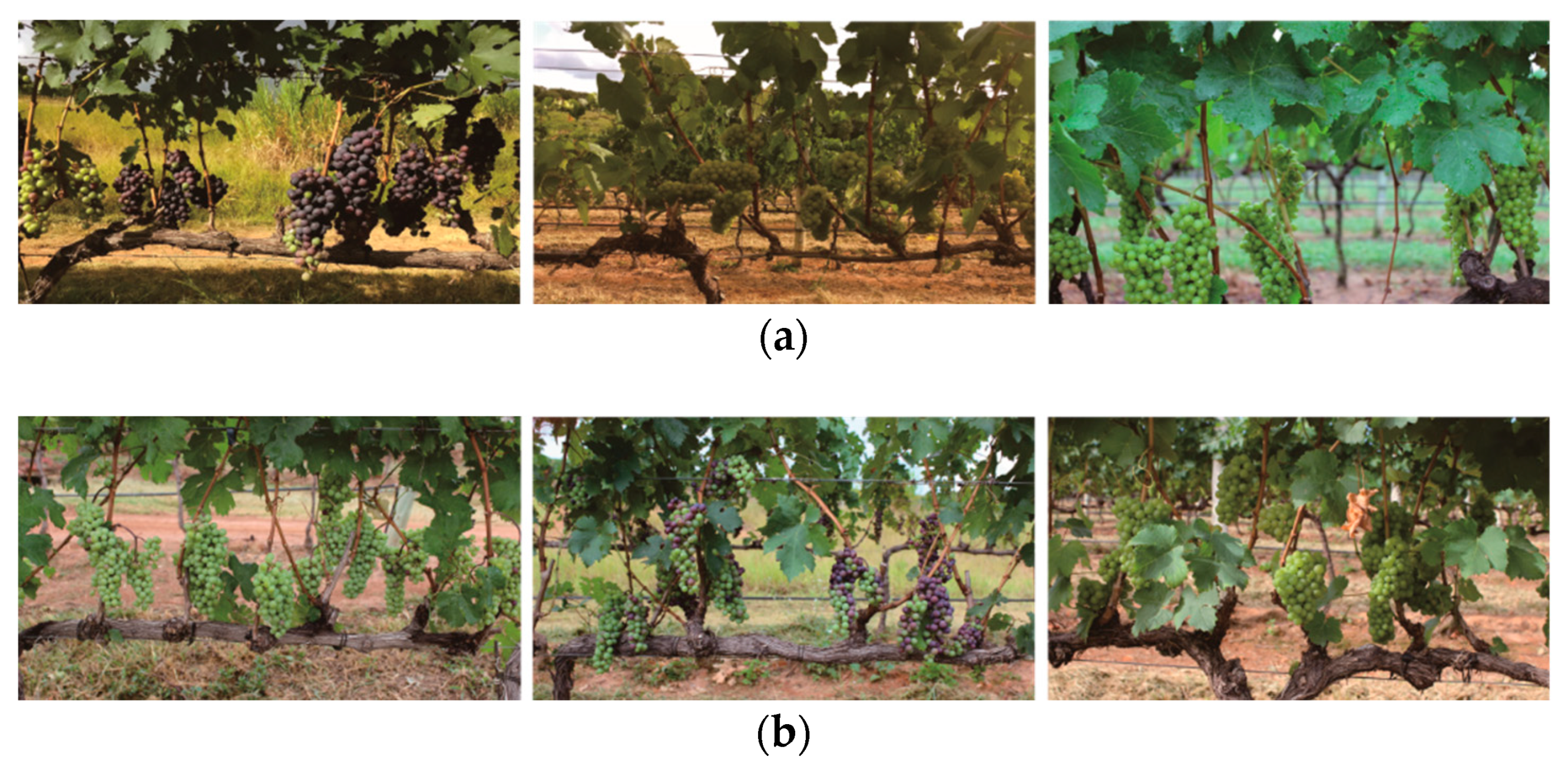
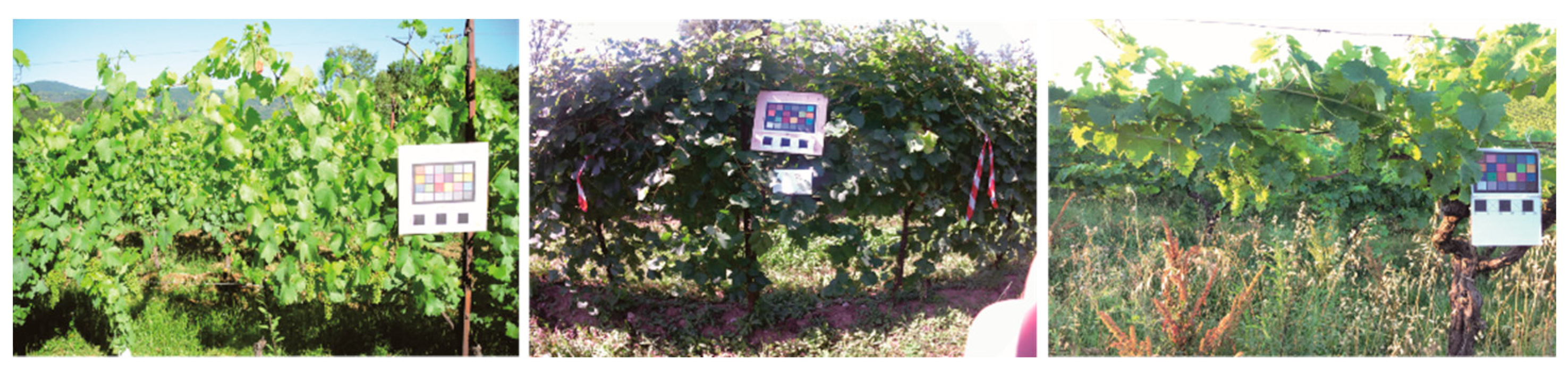
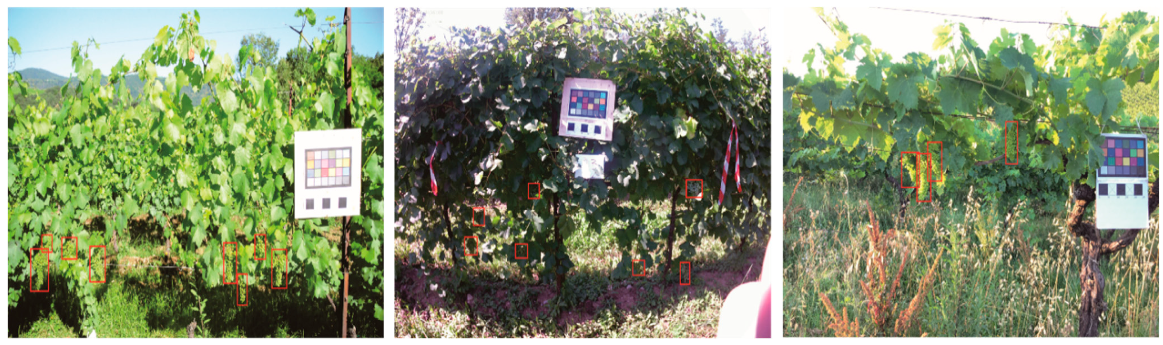
2.1. Dataset
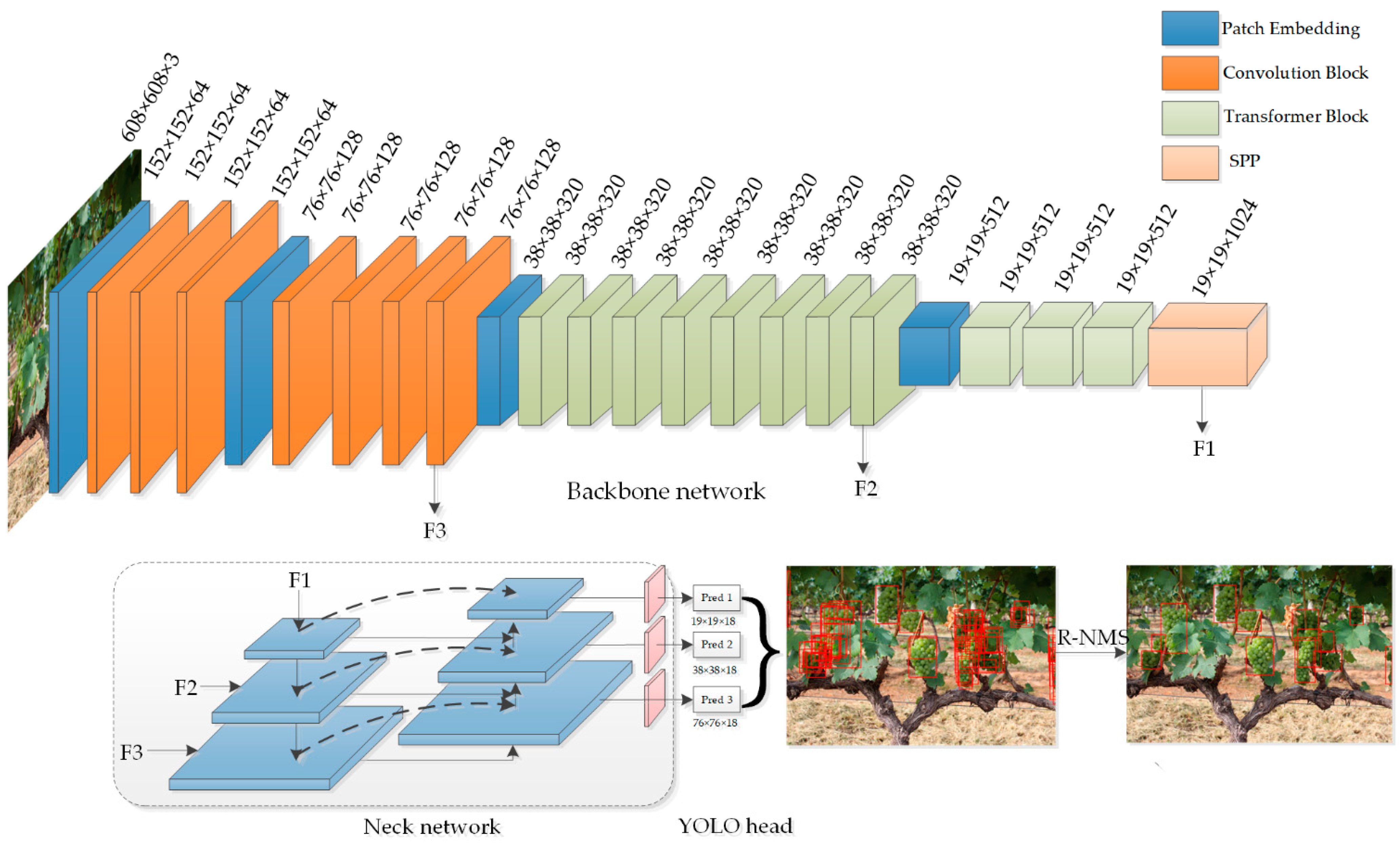
2.2. Method
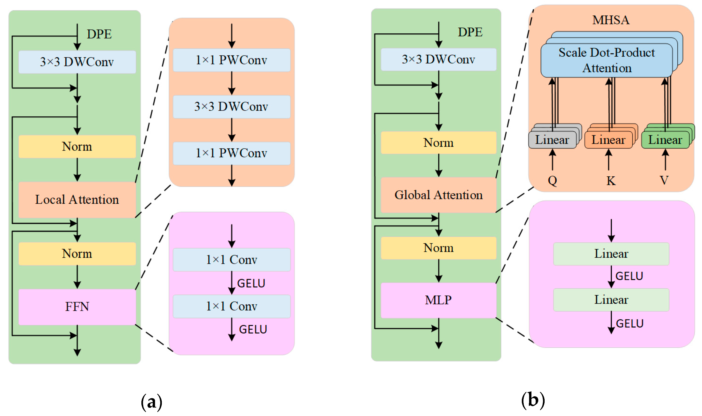
2.2.1. Backbone Network
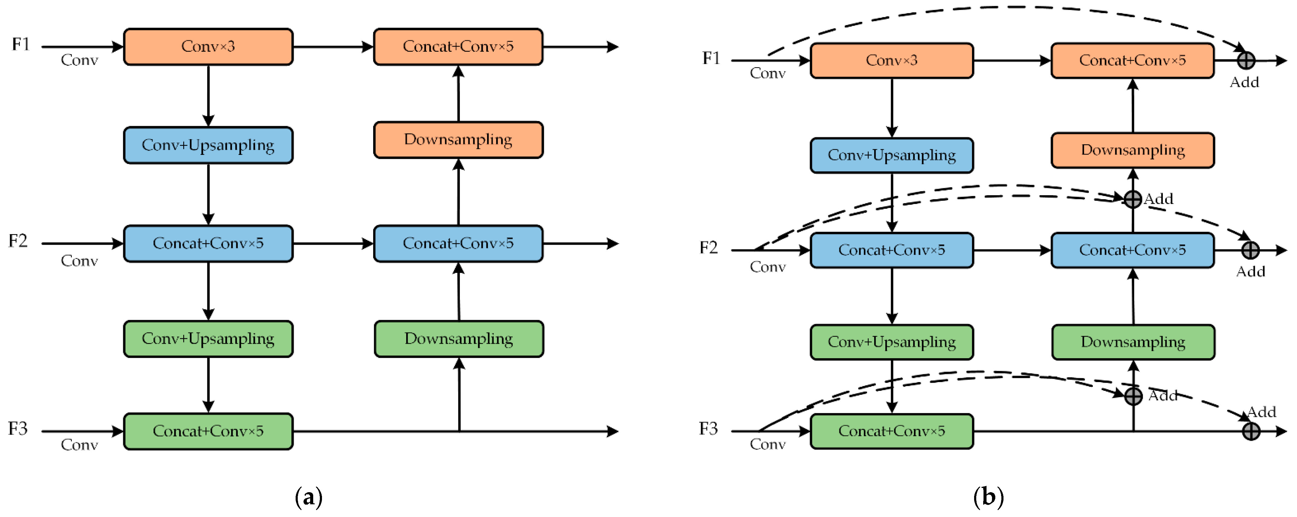
2.2.2. Neck Network
2.2.3. Bounding Box Prediction
3. Results and Discussion
3.1. Implementation Details
3.2. Evaluation Metrics
3.3. Ablation Experiments
3.4. Experimental Analysis of PANet and BiPANet
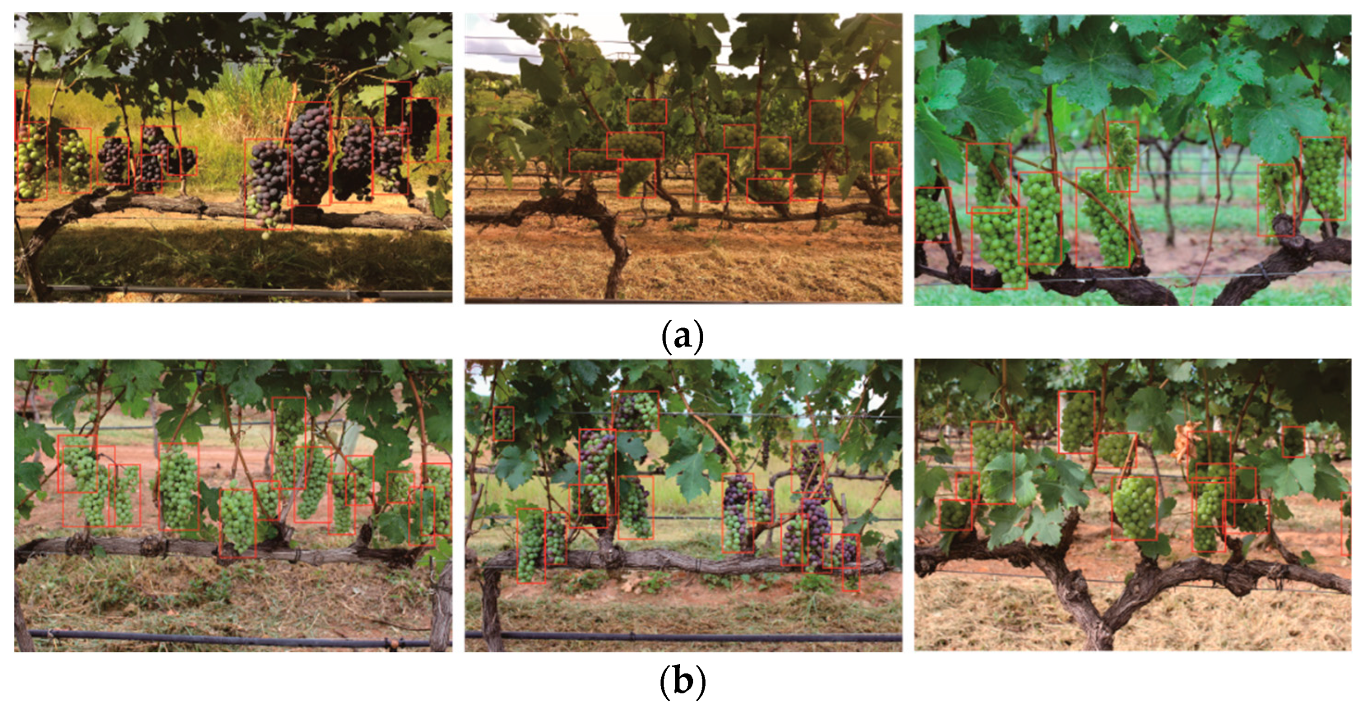
3.5. Experimental Results and Analysis
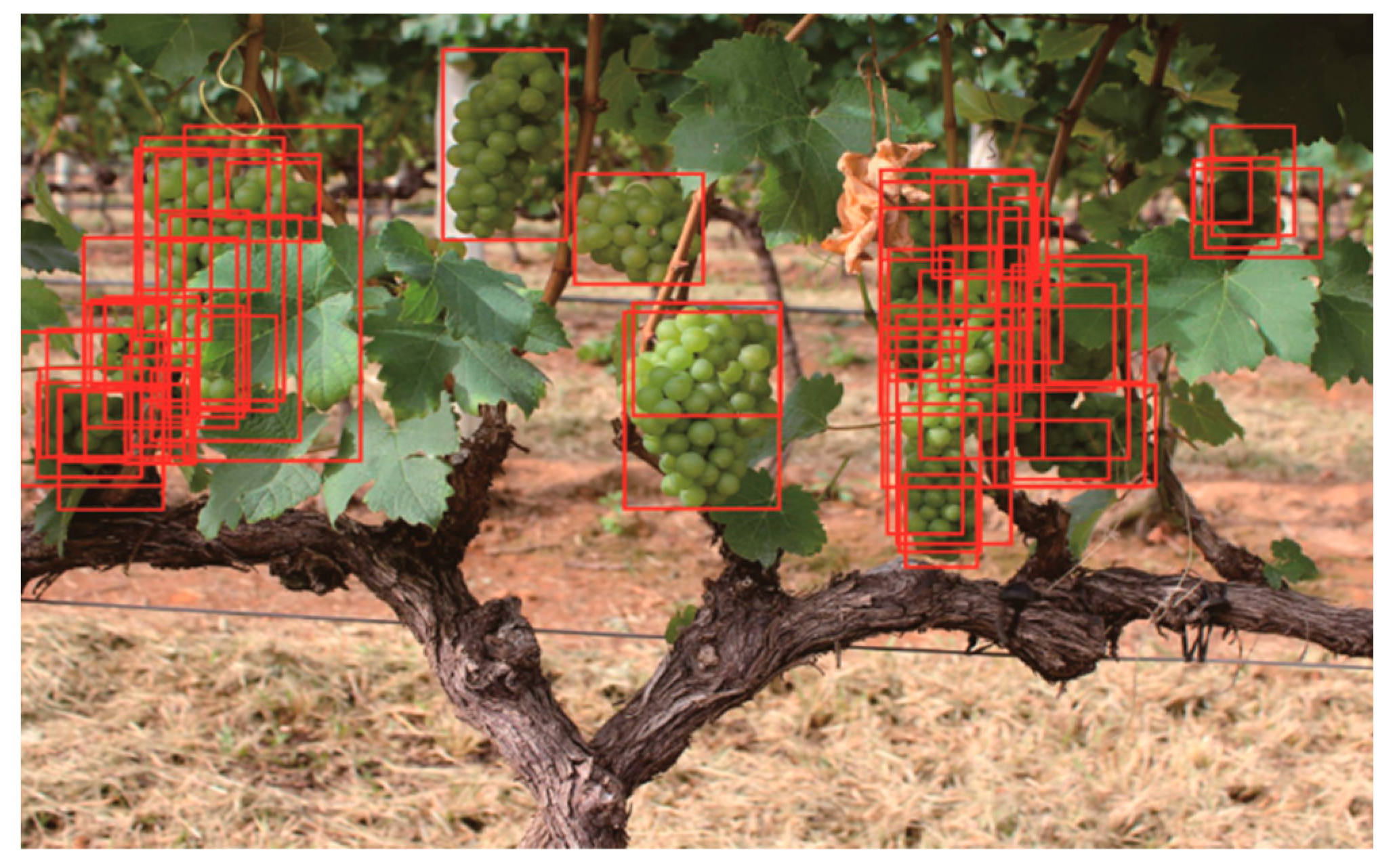
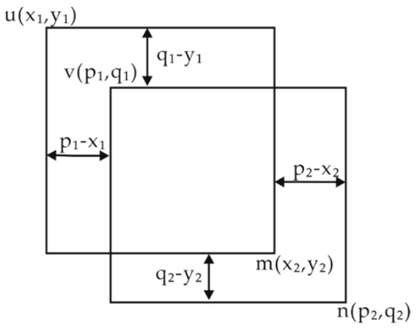
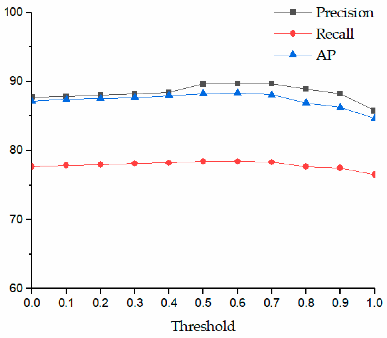
3.6. Experimental Analysis of the R-NMS Algorithm
4. Conclusions
Author Contributions
Funding
Institutional Review Board Statement
Informed Consent Statement
Data Availability Statement
Conflicts of Interest
References
- Peng, Y.; Wang, A.; Liu, J.; Faheem, M. A comparative study of semantic segmentation models for identification of grape with different varieties. Agriculture 2021, 11, 997. [Google Scholar] [CrossRef]
- Ma, B.; Jia, Y.; Mei, W.; Gao, G.; Lv, C.; Zhou, Q. Study on the recognition method of grape in different natural environment. Mod. Food Sci. Technol. 2015, 31, 145–149. [Google Scholar] [CrossRef]
- Luo, L.; Zou, X.; Wang, C.; Chen, X.; Yang, Z.; Situ, W. Recognition method for two overlapping and adjacent grape clusters based on image contour analysis. Trans. Chin. Soc. Agric. Mach. 2017, 48, 15–22. [Google Scholar] [CrossRef]
- Pérez-Zavala, R.; Torres-Torriti, M.; Cheein, F.A.; Troni, G. A pattern recognition strategy for visual grape bunch detection in vineyards. Comput. Electron. Agric. 2018, 151, 136–149. [Google Scholar] [CrossRef]
- Yan, B.; Fan, P.; Lei, X.; Liu, Z.; Yang, F. A real-time apple targets detection method for picking robot based on improved YOLOv5. Remote Sens. 2021, 13, 1619. [Google Scholar] [CrossRef]
- Liu, F.; Liu, Y.; Lin, S.; Guo, W.; Xu, F.; Zhang, B. Fast recognition method for tomatoes under complex environments based on improved YOLO. Trans. Chin. Soc. Agric. Mach. 2020, 51, 229–237. [Google Scholar] [CrossRef]
- Wang, X.; Tang, J.; Whitty, M. Data-centric analysis of on-tree fruit detection: Experiments with deep learning. Comput. Electron. Agric. 2022, 194, 106748. [Google Scholar] [CrossRef]
- Parvathi, S.; Selvi, S.T. Detection of maturity stages of coconuts in complex background using Faster R-CNN model. Biosyst. Eng. 2021, 202, 119–132. [Google Scholar] [CrossRef]
- Fu, L.; Majeed, Y.; Zhang, X.; Karkee, M.; Zhang, Q. Faster R–CNN–based apple detection in dense-foliage fruiting-wall trees using RGB and depth features for robotic harvesting. Biosyst. Eng. 2020, 197, 245–256. [Google Scholar] [CrossRef]
- Gao, F.; Fu, L.; Zhang, X.; Majeed, Y.; Li, R.; Karkee, M.; Zhang, Q. Multi-class fruit-on-plant detection for apple in SNAP system using Faster R-CNN. Comput. Electron. Agric. 2020, 176, 105634. [Google Scholar] [CrossRef]
- Peng, H.; Huang, B.; Shao, Y.; Li, Z.; Zhang, C.; Chen, Y.; Xiong, J. General improved SSD model for picking object recognition of multiple fruits in natural environment. Trans. Chin. Soc. Agric. Eng. 2018, 34, 155–162. [Google Scholar] [CrossRef]
- Zhao, D.; Wu, R.; Liu, X.; Zhao, Y. Apple positioning based on YOLO deep convolutional neural network for picking robot in complex background. Trans. Chin. Soc. Agric. Eng. 2019, 35, 172–181. [Google Scholar] [CrossRef]
- Aguiar, A.S.; Magalhães, S.A.; Dos Santos, F.N.; Castro, L.; Pinho, T.; Valente, J.; Martins, R.; Boaventura-Cunha, J. Grape bunch detection at different growth stages using deep learning quantized models. Agronomy 2021, 11, 1890. [Google Scholar] [CrossRef]
- Xiong, J.; Zheng, Z.; Liang, J.E.; Zhong, Z.; Liu, B.; Sun, B. Citrus detection method in night environment based on improved YOLO v3 Network. Trans. Chin. Soc. Agric. Mach. 2020, 51, 199–206. [Google Scholar] [CrossRef]
- Kateb, F.A.; Monowar, M.M.; Hamid, A.; Ohi, A.Q.; Mridha, M.F. FruitDet: Attentive feature aggregation for real-time fruit detection in orchards. Agronomy 2021, 11, 2440. [Google Scholar] [CrossRef]
- Wu, X.; Qi, Z.; Wang, L.; Yang, J.; Xia, X. Apple detection method based on light-YOLOv3 convolutional neural network. Trans. Chin. Soc. Agric. Mach. 2020, 51, 17–25. [Google Scholar] [CrossRef]
- Li, H.; Li, C.; Li, G.; Chen, L. A real-time table grape detection method based on improved YOLOv4-tiny network in complex background. Biosyst. Eng. 2021, 212, 347–359. [Google Scholar] [CrossRef]
- Carion, N.; Massa, F.; Synnaeve, G.; Usunier, N.; Kirillov, A.; Zagoruyko, S. End-to-end object detection with transformers. In Proceedings of the European Conference on Computer Vision, Glasgow, UK, 23–28 August 2020; pp. 213–229. [Google Scholar]
- Wang, W.; Xie, E.; Li, X.; Fan, D.-P.; Song, K.; Liang, D.; Lu, T.; Luo, P.; Shao, L. Pyramid vision transformer: A versatile backbone for dense prediction without convolutions. In Proceedings of the IEEE/CVF International Conference on Computer Vision, Virtual, 11–17 October 2021; pp. 568–578. [Google Scholar]
- Wu, H.; Xiao, B.; Codella, N.; Liu, M.; Dai, X.; Yuan, L.; Zhang, L. Cvt: Introducing convolutions to vision transformers. In Proceedings of the IEEE/CVF International Conference on Computer Vision, Virtual, 11–17 October 2021; pp. 22–31. [Google Scholar]
- Jiang, B.; Luo, R.; Mao, J.; Xiao, T.; Jiang, Y. Acquisition of localization confidence for accurate object detection. In Proceedings of the European Conference on Computer Vision, Munich, Germany, 8–14 September 2018; pp. 784–799. [Google Scholar]
- Neubeck, A.; Van Gool, L. Efficient non-maximum suppression. In Proceedings of the 18th International Conference on Pattern Recognition, Hong Kong, China, 20–24 August 2006; pp. 850–855. [Google Scholar]
- Bochkovskiy, A.; Wang, C.Y.; Liao, H.Y.M. Yolov4: Optimal speed and accuracy of object detection. arXiv 2020, arXiv:2004.10934. [Google Scholar]
- Li, K.; Wang, Y.; Zhang, J.; Gao, P.; Song, G.; Liu, Y.; Li, H.; Qiao, Y. Uniformer: Unifying convolution and self-attention for visual recognition. arXiv 2022, arXiv:2201.09450. [Google Scholar]
- Liu, S.; Qi, L.; Qin, H.; Shi, J.; Jia, J. Path aggregation network for instance segmentation. In Proceedings of the IEEE Conference on Computer Vision and Pattern Recognition, Salt Lake City, UT, USA, 18–22 June 2018; pp. 8759–8768. [Google Scholar]
- Santos, T.; de Souza, L.; dos Santos, A.; Sandra, A. Embrapa Wine Grape Instance Segmentation Dataset–Embrapa WGISD. Zenodo. 2019. Available online: https://doi.org/10.5281/zenodo.3361736 (accessed on 23 June 2021).
- Sozzi, M.; Cantalamessa, S.; Cogato, A.; Kayad, A.; Marinello, F. wGrapeUNIPD-DL: An open dataset for white grape bunch detection. Data Brief. 2022, 43, 108466. [Google Scholar] [CrossRef]
- Sandler, M.; Howard, A.; Zhu, M.; Zhmoginov, A.; Chen, L.-C. Mobilenetv2: Inverted residuals and linear bottlenecks. In Proceedings of the IEEE Conference on Computer Vision and Pattern Recognition, Salt Lake City, UT, USA, 18–22 June 2018; pp. 4510–4520. [Google Scholar]
- Li, S.; Zhang, G.; Luo, Z.; Liu, J. Dfan: Dual feature aggregation network for lightweight image super-resolution. Wirel. Commun. Mob. Comput. 2022, 2022, 1–13. [Google Scholar] [CrossRef]


| Categories | Species of Grapes | Total Number | Number of the Training Set | Number of the Test Set | ||||
|---|---|---|---|---|---|---|---|---|
| Chardonnay | Cabernet Franc | Cabernet Sauvignon | Sauvignon Blanc | Syrah | ||||
| Number of images | 65 | 65 | 57 | 65 | 48 | 300 | 240 | 60 |
| Number of labeled grapes | 840 | 1069 | 643 | 1317 | 563 | 4432 | 3500 | 932 |
| Categories | Total Number | Number of the Training Set | Number of the Test Set |
|---|---|---|---|
| Number of images | 268 | 214 | 54 |
| Number of labeled grapes | 2155 | 1744 | 411 |
| Stage | Input | Operation | Output |
|---|---|---|---|
| Stage 1 | 608 × 608 × 3 | 152 × 152 × 64 | |
| Stage 2 | 152 × 152 × 64 | 76 × 76 × 128 | |
| Stage 3 | 76 × 76 × 128 | 38 × 38 × 320 | |
| Stage 4 | 38 × 38 × 320 | 19 × 19 × 512 | |
| Parameters | Values |
|---|---|
| Image resolution | 608 × 608 |
| Batch size 1 | 8 |
| Batch size 2 | 4 |
| Learning rate 1 | 0.001 |
| Learning rate 2 | 0.0001 |
| Weight decay rate 1 | 0.0005 |
| Weight decay rate 2 | 0.0005 |
| Optimizer | Adam |
| Epochs | 150 |
| Methods | Uniformer | PANet-Lite | BiPANet | R-NMS | Precision | Recall | F1 | mAP | Params | FLOPs | FPS |
|---|---|---|---|---|---|---|---|---|---|---|---|
| A | ✗ | ✗ | ✗ | ✗ | 87.2% | 76.5% | 81.5% | 86.0% | 64.0 M | 63.9 G | 38 |
| B | ✓ | ✗ | ✗ | ✗ | 87.4% | 77.5% | 82.2% | 87.0% | 54.0 M | 51.2 G | 44 |
| C | ✓ | ✓ | ✗ | ✗ | 87.2% | 77.2% | 81.9% | 86.7% | 34.8 M | 36.3 G | 50 |
| D | ✓ | ✗ | ✓ | ✗ | 87.7% | 77.7% | 82.4% | 87.3% | 34.8 M | 36.3 G | 50 |
| E | ✓ | ✗ | ✗ | ✓ | 87.9% | 78.1% | 83.1% | 87.5% | 54.0 M | 51.2 G | 39 |
| Our method | ✓ | ✗ | ✓ | ✓ | 88.6% | 78.3% | 83.1% | 87.7% | 34.8 M | 36.3 G | 46 |
| Methods | Uniformer | PANet-Lite | BiPANet | R-NMS | Precision | Recall | F1 | mAP | Params | FLOPs | FPS |
|---|---|---|---|---|---|---|---|---|---|---|---|
| A | ✗ | ✗ | ✗ | ✗ | 84.3% | 60.6% | 70.5% | 70.4% | 64.0 M | 63.9 G | 38 |
| B | ✓ | ✗ | ✗ | ✗ | 85.0% | 61.8% | 71.6% | 72.0% | 54.0 M | 51.2 G | 44 |
| C | ✓ | ✓ | ✗ | ✗ | 85.5% | 60.4% | 70.8% | 71.7% | 34.8 M | 36.3 G | 50 |
| D | ✓ | ✗ | ✓ | ✗ | 85.2% | 62.4% | 72.0% | 72.4% | 34.8 M | 36.3 G | 50 |
| E | ✓ | ✗ | ✗ | ✓ | 85.4% | 62.0% | 71.8% | 72.2% | 54.0 M | 51.2 G | 39 |
| Our method | ✓ | ✗ | ✓ | ✓ | 85.7% | 62.3% | 72.2% | 72.8% | 34.8 M | 36.3 G | 46 |
| Methods | Precision | Recall | F1 | mAP | Params | FLOPs | FPS |
|---|---|---|---|---|---|---|---|
| Faster R-CNN | 72.8% | 51.6% | 60.4% | 66.3% | 28.3 M | 196.5 G | 20 |
| SSD | 85.1% | 75.9% | 80.2% | 85.2% | 24.4 M | 124.6 G | 46 |
| RetinaNet | 78.9% | 63.8% | 70.1% | 74.4% | 36.5 M | 74.7 G | 36 |
| YOLOv3 | 83.4% | 77.7% | 80.4% | 84.2% | 61.6 M | 70.0 G | 44 |
| YOLOv4 | 87.2% | 76.5% | 81.5% | 86.0% | 64.0 M | 63.9 G | 38 |
| YOLOx | 85.6% | 80.4% | 82.9% | 86.9% | 54.2 M | 70.1 G | 44 |
| Our method | 88.6% | 78.3% | 83.1% | 87.7% | 34.8 M | 36.3 G | 46 |
| Methods | Precision | Recall | F1 | mAP | Params | FLOPs | FPS |
|---|---|---|---|---|---|---|---|
| Faster R-CNN | 65.7% | 40.2% | 49.9% | 43.2% | 28.3 M | 196.5 G | 20 |
| SSD | 72.8% | 51.9% | 60.6% | 56.2% | 24.4 M | 124.6 G | 46 |
| RetinaNet | 67.7% | 46.1% | 54.9% | 45.7% | 36.5 M | 74.7 G | 36 |
| YOLOv3 | 83.0% | 53.6% | 65.1% | 65.6% | 61.6 M | 70.0 G | 44 |
| YOLOv4 | 84.3% | 60.6% | 70.5% | 70.4% | 64.0 M | 63.9 G | 38 |
| YOLOx | 79.6% | 65.4% | 71.8% | 72.6% | 54.2 M | 70.1 G | 44 |
| Our method | 85.7% | 62.3% | 72.2% | 72.8% | 34.8 M | 36.3 G | 46 |
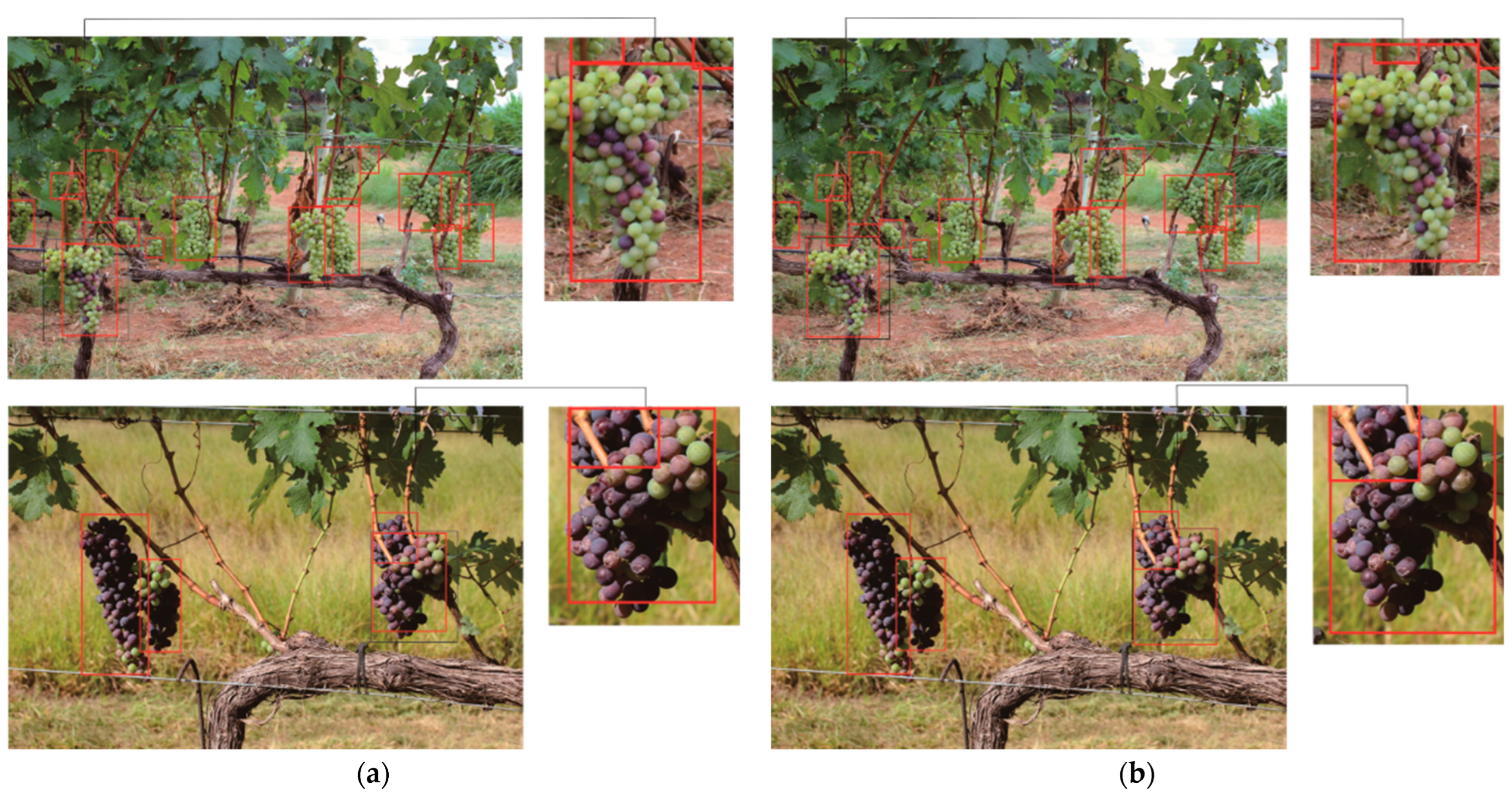
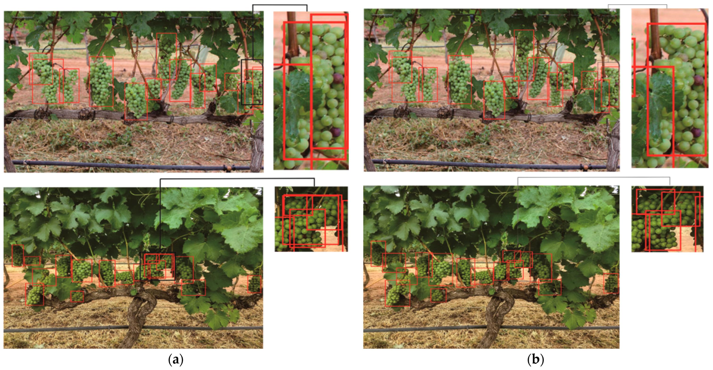
| Methods | Grape Detection Results in Figure 8 | Grape Detection Results in Figure 9 | ||||
|---|---|---|---|---|---|---|
| Number of TP Bounding Boxes | Number of FP Bounding Boxes | Number of FN Bounding Boxes | Number of TP Bounding Boxes | Number of FP Bounding Boxes | Number of FN Bounding Boxes | |
| Faster R-CNN | 68 | 22 | 41 | 15 | 11 | 10 |
| SSD | 69 | 6 | 10 | 12 | 0 | 0 |
| RetinaNet | 66 | 17 | 26 | 14 | 1 | 0 |
| YOLOv3 | 68 | 8 | 7 | 17 | 0 | 0 |
| YOLOv4 | 70 | 3 | 5 | 19 | 1 | 2 |
| YOLOx | 72 | 5 | 3 | 19 | 0 | 0 |
| Our method | 73 | 1 | 3 | 19 | 0 | 0 |
Publisher’s Note: MDPI stays neutral with regard to jurisdictional claims in published maps and institutional affiliations. |
© 2022 by the authors. Licensee MDPI, Basel, Switzerland. This article is an open access article distributed under the terms and conditions of the Creative Commons Attribution (CC BY) license (https://creativecommons.org/licenses/by/4.0/).
Share and Cite
Su, S.; Chen, R.; Fang, X.; Zhu, Y.; Zhang, T.; Xu, Z. A Novel Lightweight Grape Detection Method. Agriculture 2022, 12, 1364. https://doi.org/10.3390/agriculture12091364
Su S, Chen R, Fang X, Zhu Y, Zhang T, Xu Z. A Novel Lightweight Grape Detection Method. Agriculture. 2022; 12(9):1364. https://doi.org/10.3390/agriculture12091364
Chicago/Turabian StyleSu, Shuzhi, Runbin Chen, Xianjin Fang, Yanmin Zhu, Tian Zhang, and Zengbao Xu. 2022. "A Novel Lightweight Grape Detection Method" Agriculture 12, no. 9: 1364. https://doi.org/10.3390/agriculture12091364
APA StyleSu, S., Chen, R., Fang, X., Zhu, Y., Zhang, T., & Xu, Z. (2022). A Novel Lightweight Grape Detection Method. Agriculture, 12(9), 1364. https://doi.org/10.3390/agriculture12091364