A Machine Learning Model for Early Prediction of Crop Yield, Nested in a Web Application in the Cloud: A Case Study in an Olive Grove in Southern Spain

Abstract

Predictive systems are a crucial tool in management and decision-making in any productive sector. In the case of agriculture, it is especially interesting to have advance information on the profitability of a farm. In this sense, depending on the time of the year when this information is available, important decisions can be made that affect the economic balance of the farm. The aim of this study is to develop an effective model for predicting crop yields in advance that is accessible and easy to use by the farmer or farm manager from a web-based application. In this case, an olive orchard in the Andalusia region of southern Spain was used. The model was estimated using spatio-temporal training data, such as yield data from eight consecutive years, and more than twenty meteorological parameters data, automatically charged from public web services, belonging to a weather station located near the sample farm. The workflow requires selecting the parameters that influence the crop prediction and discarding those that introduce noise into the model. The main contribution of this research is the early prediction of crop yield with absolute errors better than 20%, which is crucial for making decisions on tillage investments and crop marketing.

1. Introduction

Spain is the country with the largest olive grove area in the world, reaching 2.5 Mha, 60% of which is concentrated in the Andalusia Region, in southern Spain [1], where the climate provides ideal growing conditions for olive trees [2]. Olive growing is therefore an important economic factor for Spain, especially for Andalusia. Moreover, olive oil is known worldwide for its culinary contributions and its health benefits. In fact, olive oil is included in the Mediterranean Diet Pyramid, which underlines the importance of the foods making up the principal food groups [3].

Olive crop is undergoing constant growth on an international level due to a steady worldwide increase of the olive growing area and improvements in irrigation systems and technological advances [4,5]. In the current political–financial framework for agriculture, the new Common Agricultural Policy (CAP) reforms are geared towards achieving environmental objectives such as fighting climate change and supporting European farmers in achieving a sustainable and competitive agricultural sector by focusing on the digitalization of the olive sector. In this process, agriculture 4.0 could play a key role. This term refers to the technological revolution that characterizes the modern agricultural sector, based on the widespread sharing of digital technologies, smart farming, and knowledge-based production methods [6,7]. This technology has enormous potential, as these tools can be applied to a wide variety of farming systems and require less financial investment compared to machinery or heavy equipment. Technological improvement increases the quantity of outputs relative to the quantity of inputs and shifts the “technological frontier”. This displacement translates into higher productivity.

Information technologies and Artificial Intelligence (AI) are key in multiple sectors [8,9], since they are based on the optimization of production systems and marketing and help in the decision-making process [10,11]. Machine Learning (ML), a branch of artificial intelligence, is a practical approach used in many fields, including agriculture, for several years [12]. Today, ML remains the most common and popular approach to AI in the field of agriculture and beyond [13]. The valuable knowledge shared between farmers and experts in these technologies allows valuable information to be inferred for making the right decisions in the agricultural sector and improving crop productivity and environmental sustainability, the main objectives of the new agricultural policies. In this sense, the reality for the farmer, and especially for the olive farmer, is that due to numerous reasons, his hard work does not always result in maximum crop yields. Crop yields depend on several factors, such as soil, climate, irrigation, rainfall, Pesticides, fertilizers, tillage, temperature, and the harvest of last year. The farmer or farm manager often needs to make decisions for which having advance information on future harvest would help to define the best management strategy [14]. The olive sector is not an exception, and currently the actors involved must make decisions every day related to agricultural practices and management, with the consequent economic investment that this implies in the farms (fertilizer, tillage, etc.). Additionally, the farmer or the farm manager has to make decisions about the best way to market the oil. This is an important matter that requires a comprehensive and in-depth knowledge of the current state of the farm and how it can evolve in the medium and long term. Consequently, the need to carry out an analysis of variables from different sources and nature is evident. From the point of view of optimizing the farmer’s economic resources, the most useful thing for him is to know well in advance, before making the investment, what the yield of his crop will be depending on the practices he performs or does not perform during each season. This information is interesting for other professionals who are part of the olive sector in addition to being useful for farmers. As an example, advance information on harvest quantity can be key for insurance companies to know the risk of the insured property, and based on this, establish their rates. In the case of those actors with responsibility for marketing the oil, it is important to determine the best time to carry out the sale or purchase, or to establish their storage forecasts. In summary, a system capable of making an early prediction about the harvest, that is, in January, February, or even March, with a low ratio of error is key to designing a correct marketing strategy.

Crop yield prediction is one of the challenging problems in precision agriculture; however, as Xu et al. (2019) [15] indicates, this is not a trivial task. Nowadays, crop yield prediction models can estimate the actual values reasonably, but a better performance in yield prediction is still desirable [16]. Numerous authors have emphasized for years the importance of the quantitative forecasting of crop yields, considering it as a valuable tool in the support of the farmers in the olive sector [17]. There are numerous investigations about the use of long-term data series to carry out crop-forecasting technique for numerous species, also in the olive grove [18,19,20]. In this research, the close relationships between pollen emission and fruit production are widely studied. Nevertheless, the final fruit production is influenced by several weather and agronomic conditions during both the pre-flowering period and the time period between flowering and harvest, such as water deficit, temperature extremes, and phytopathological problems [21,22,23].

There are several studies in olive crop yield prediction, and most of them are based on the predictive value of pollen emission levels [16,21,22,23,24,25,26,27,28]. In these studies, basic parameters of pollen levels are taken into account, in addition to other factors of temperature, rainfall, and relative humidity. Regression analysis is performed in the last study. This model presents results with an error of 0.96% in July. It must be considered that generally, in traditional olive groves, the olives were harvested between the months of December and January, and it is in January that the tillage work begins. In other words, these models are very accurate, but reliable prediction is made after pollination, which occurs at a very advanced stage of the agricultural year: April, May, or June. Therefore, it is a very reliable model, but it provides a very late prediction (only 5 months after the olive harvest). More recently, other prediction works, such as the novel study presented by López-Bernal et al., 2021 [29], estimate a conceptual model for predicting fruit oil content. The results provide useful information for the farmer; it is about helping to establish optimal harvesting periods. However, the purpose of the prediction is not aimed at the objective set out above.

The basis of the predictive challenge is that it is used by the farmer or farm manager. Often predictive systems are implemented on applications that are unfriendly and too complex, and only their developers know how to operate them. As a result, these systems are not used. In order for these tools to be successful, it is essential that the expert system is accessible with a user-friendly interface.

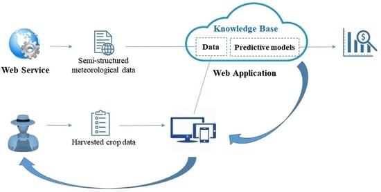
Therefore, this system is additionally integrated into a web application with cloud deployment. This system is fed with public data from web services of government agencies and is freely accessible. Additionally, data provided by the farmer or farm manager himself complete the data set. The aim is to generate a predictive model that provides information at an early stage, at the beginning of the year, on the amount of olive crop that will be harvested that year. The innovation of this work lies in the early stage of the prediction and in the combination of variables downloaded from official web services, these being web services belonging to official meteorological institutions. Other essential data to generate the predictive models are the values of the amount of harvest collected in previous years. This information is crucial for all the agents involved in the olive sector, as it helps to make the right strategic decisions, both for the initial tillage phase and for the final oil marketing phase. For this reason, the predictive model has been integrated into a web application that is accessible and simple for users. The proposed method represents a disruption in relation to the most advanced methods, as previous contributions provide a harvest prediction based on pollen data and remote observation of the fruit at the stages closest to harvest. Our solution does not need these data that require field data collection campaigns and arduous processing, but rather information available on the internet and harvest quantity data collected from previous years.

Objectives and Hypotheses

In relation to the review of the state of the art, there are works related to the prediction of olive crop yield; however, there is very little research on prediction at an early stage of the agricultural season. These data are of great interest in the olive-growing sector, as they provide information in advance that allows for adequate economic and sustainable planning by all the actors involved in this sector. However, for the results of this research to be really useful, it is necessary that this prediction be transferred to the productive sector, i.e., the end user. Thus, this work proposes the design of a tool that allows this predictive model to be accessible. This research hypothesised the generation of an early prediction of olive crop yield using new models from ML algorithms. In addition, the idea is that this information should reach the farmer or person in charge of managing olive orchards, which is why the aim is to integrate this model into a tool that is easy to use for these users. Thus, this work has a main objective which is: (1) to generate an early prediction model of olive harvest yield, and as a complement to the previous objective: (2) to nest this ML model in a cloud-based web application to improve the convenience, accessibility, and use of the proposed software by the end users.

The scientific hypothesis of this work is focused on the aim of this paper, which is to predict, at an early stage, the amount of kilograms of crop that the farmer will harvest using several regression algorithms. The process takes as a starting point the hypothesis that there are several variables related to the harvest quantity, mainly the previous year’s harvest and a number of climatic variables. In this sense, as described in the introduction, there are several studies that corroborate this relationship. For all these reasons, ML techniques are used in a supervised learning study, where all the predictor variables are labelled.

There are numerous regression algorithms, such as Linear Regression, Logistic Regression, Generalised Regression Model, One-Class Support Vector Machine (SVM), etc. In this study, a priori the nature of the variables is unknown and there are few training data available (we have harvest data collected over eight years); therefore, linear and non-linear regression algorithms are used, as follows:

• Linear: purely linear algorithms have a great strength due to their characteristics and simplicity, as they are calculated with a simple weighted sum of the variables:

y = β₀ + β₁x₁ + … + β_px_p + ϵ

(1)

The first algorithm selected in this study is Generalised Linear Models (GLM), which works mathematically as the weighted sum of the features with the mean value of the distribution assumed using the link function g, which can be chosen flexibly depending on the type of result.

g(EY(y|x)) = β₀ + β₁x₁ + …β_px_p

(2)

In other words, this algorithm is an extension of the linear algorithms allowing to model linear or normal distributions and non-constant variances.

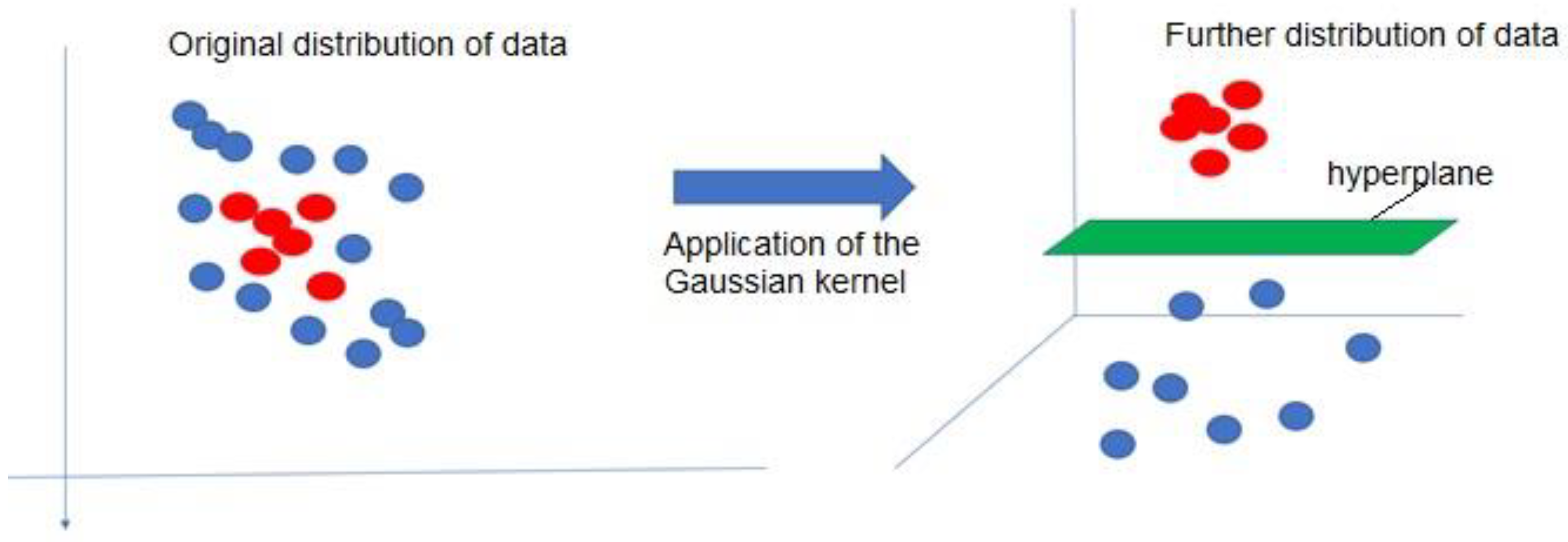
Another Linear algorithm selected is SVM, which has the great advantage of being able to be used with different Kernels. Kernels allow the data to be distributed in a hyperplane according to a function, which makes it easier for the algorithm to adapt to the nature of the data, allowing infinite transformations, Figure 1.

In this study, we work with SVM with Linear Kernel. When using the Linear kernel, the following transformation is performed:

K(x,x′) = x⋅x′

(3)

This algorithm has the advantage that it fits very well if the nature of the data is linear, and if there are many predictor variables (as in our case). It should be noted that in this algorithm, there is no upper limit on the number of predictor attributes; the only limitations are those imposed by the hardware. In this study, we have a limited set of training data, since we have a limited number of years with harvest quantity data, but we do have a large number of predictor variables.

• Non-linear: in this case, the SVM algorithm is applied with a Gaussian Kernel. This kernel applies the following transformation to the data:

K(x,x′) = exp(−γ||x − x′||2)

(4)

The value of γ controls the behavior of the kernel. When it is very small, the final model is equivalent to that obtained with a linear kernel, and as its value increases the data becomes more distant, forming a Gaussian bell in the hyperplane, adapting very well when the nature of the data does not have a linear distribution.

In summary, these are the advantages of these three algorithms in this study, based on the hypothesis of a priori ignorance of the relationship between the variables with the target attribute and also taking into account that the training data we have are limited and the predictor variables are numerous. Furthermore, the complexity of these algorithms means that the relationship between the attributes used cannot be described by means of a specific equation.

2. Materials and Methods

The model implemented is based on the application of different data mining techniques to generate predictive models of the amount of olive crop that will be harvested. Data mining arises from the convergence of various disciplines, such as computer science, statistics, artificial intelligence, database technology, etc. Data mining is a logical process of finding useful information to discover useful data. Once the information and patterns are found, they can be used to make decisions for developing the business; in this case, this study seeks the relationship between the amount of olive crop harvested in a given year and multiple variables, such as the historical yield data and meteorological variables of previous years. Data mining techniques are lengthily functional to the agricultural sector [30]. It is used to examine a large dataset and establish serviceable classifications and patterns in this dataset. The overall aim of the data mining method is to extract useful information from the dataset and exchange it into an explicable structure for additional use.

The methodology followed in this work is sequenced in several phases, from the data understanding, data preparation, and generation of the models to the validation and implementation of the models. The output data of the model is the amount of olive crop, that is, the number of kg of olives that will be collected in each campaign on the farm under study. This is an unknown variable, but it can be deduced from other variables that are known and that are directly or inversely related to the target. In this sense, the study is based on a supervised analysis of data mining, where the value of an unknown variable is deduced from a few known variables.

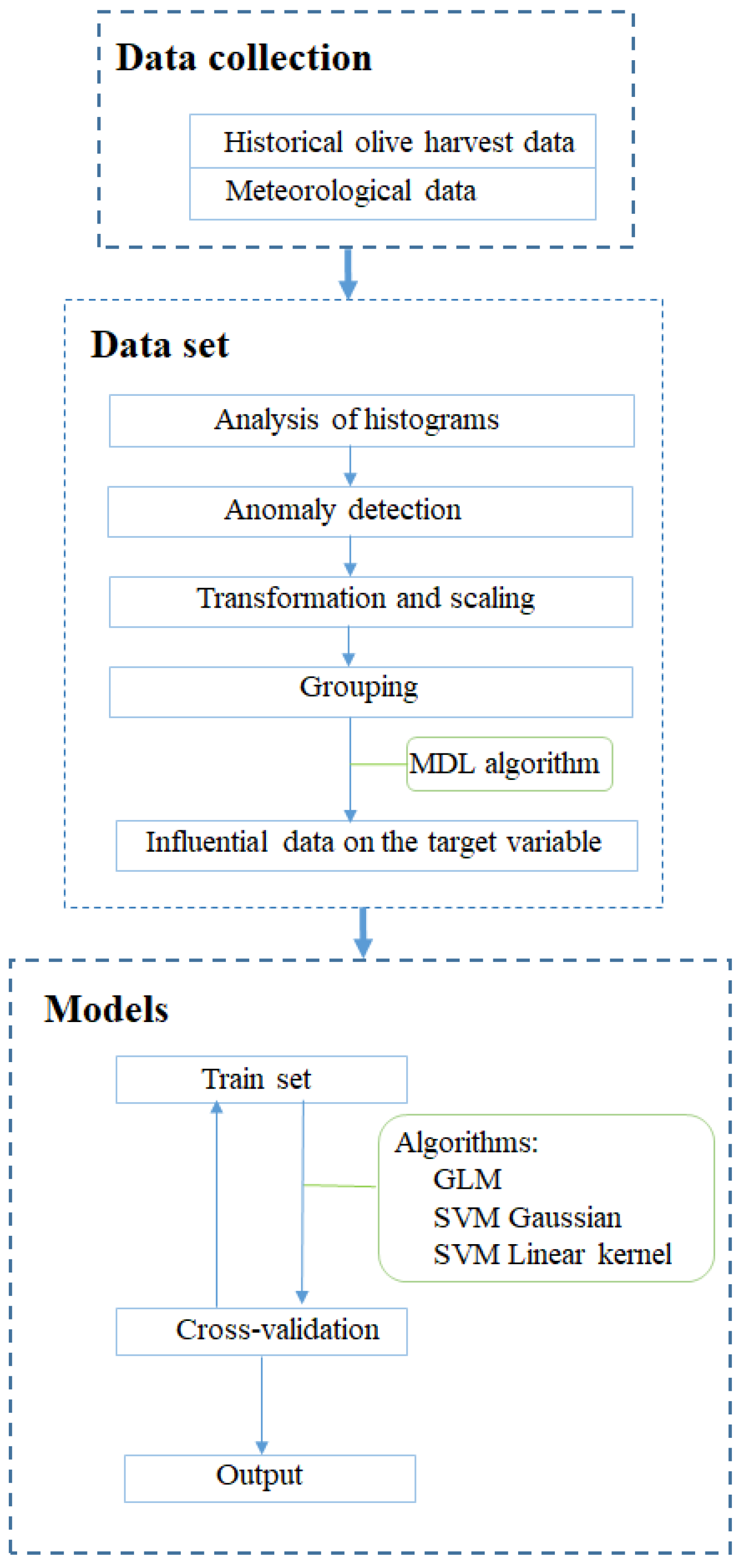
The general flow of the methodology carried out is composed of data mining algorithms and techniques used as follows in each phase:

• Extraction and loading of data. Meteorological data are downloaded from web servers for public use. Olive crop harvested data is provided by the owner of the farm. Both will be uploaded to the database management system.
• First analysis of data. All data are explored and analysed using distribution techniques (histograms), with the objective of reviewing the data and cleaning those whose dispersion or variability may cause inconsistencies in the study.
• Anomaly detection. The detection of the anomalies is implemented as a class classification algorithm, where the algorithm is able to predict, with a certain probability, whether a record of the data is typical of the distribution. The objective of this phase is to identify those cases that are not common within our information.
• Transformations of data. In this section, both the yield data and the meteorological data are transformed, i.e., adapting formats, units, rescaled, etc, so that they could be optimally exploited by predictive models.
• Grouping of data. The information downloaded is aggregated monthly; therefore, the rest of the data to be added to the study should be aggregated in the same way.
• Integration of data. For our work, we have heterogeneous information that comes from different sources. The farmer indicates the annual net olive crop harvest, and meteorological information is available for the area where the farm is located. Thus, in order to carry out the data mining study, it is necessary to integrate all the information in a single source that serves as the input for the predictive models.
• Detection of the level of influence of the input attributes on the target attribute. Before generating the model, the influence of each attribute on the target attribute (kg of olives, the olive crop harvest) is analyzed in order to include or exclude attributes from the study based on their level of influence on the prediction.
• Application of regression algorithms [31,32,33]. To perform the crop harvest prediction, different regression algorithms are tested. The goal of regression analysis is to determine the parameter values from a function that best fit a set of observational data. There are different families of regression functions and different ways of measuring error. This study uses:

  •

  Linear regression: this technique can be used if the relationship between variables can be approximated to a straight line. This is used to predict the value of a variable based on the value of another variable. The variable you want to predict is called the dependent variable. The variable you are using to predict the other variable’s value is called the independent variable.

  •

  Nonlinear regression: it is a nonlinear combination of the model parameters and depends on one or more independent variables. It relates the two variables in a nonlinear, curved, relationship. The data are fitted by a method of successive approximations.

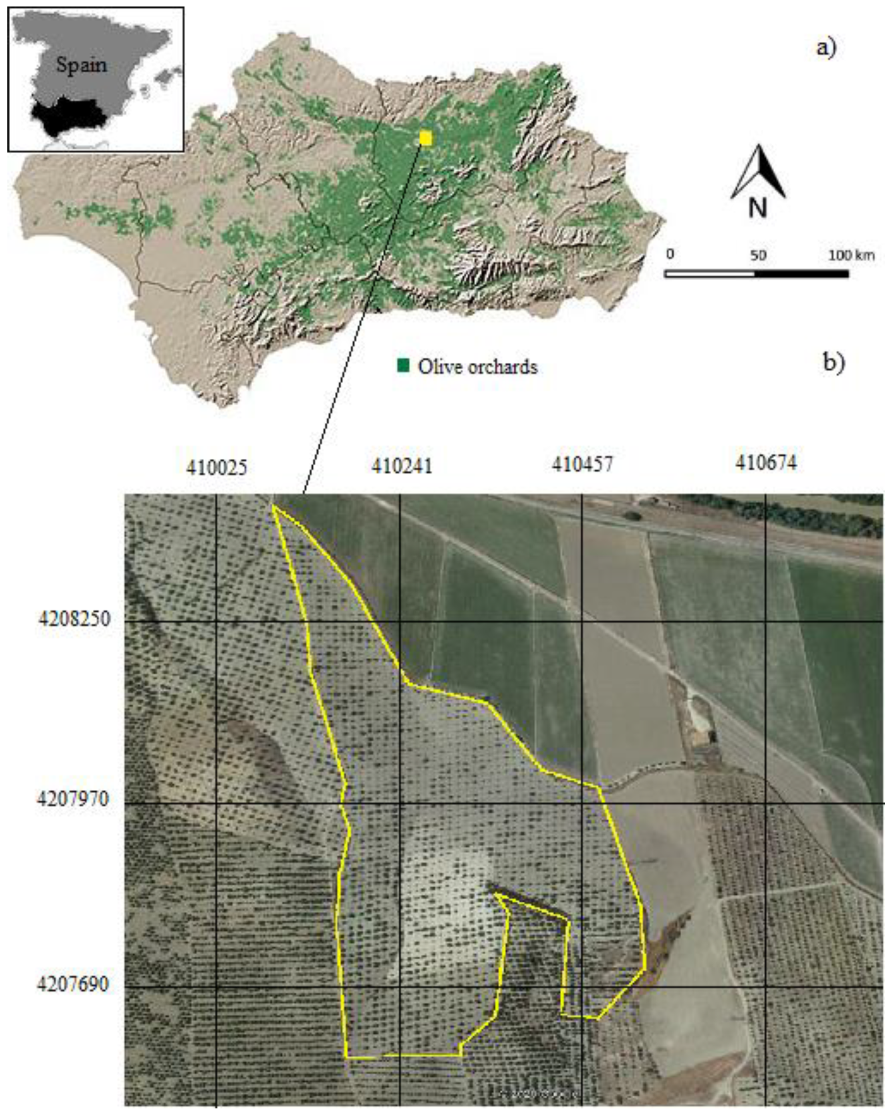
2.1. Experimental Site

This study was conducted in an olive growing farm situated in Jaén (Andalusia), which is located in the southern area of Spain, Figure 2. The perfect habitat for the cultivation of the olive tree is between latitudes 30° and 45°, so the Mediterranean climate and specifically the dry and hot summer climate of Jaén is perfect for its healthy growth and its greater use in harvest. The farm is an unirrigated olive orchard situated in 38°00′ N, 4°01′ W. The olive orchard studied is 3, 5 ha with 330 olive trees of similar properties; they all are about 25 years old and their mean fruit harvest is 60 kg/year. This is a traditional irrigated olive grove, in which the trees have two trunks and are planted at a distance of 10 m from each other. Cultivation methods include ploughing or other intensive tillage, such as harrowing to remove most of the plant residue cover. The main objective of this type of tillage is to keep the top cover of the olive grove free of weeds. After harvesting, from December to February, a 15 cm deep moldboard ploughing is carried out, which is essential to prepare the topsoil to absorb rainwater. The frequency of ploughing depends on rainfall. In summer, surface ploughing is carried out to increase the storage capacity of surface water in the soil but keep the organic substance at the surface level.

Regarding the rest of the treatment of the farm, pruning is carried out after harvesting, followed by fertilization with water-soluble fertilizers containing nitrogen, phosphorus, potassium, sulphur, magnesium, and micronutrients.

2.2. Dataset

Any predictive study requires the availability of adequate data in order to guarantee a quality prediction. Regarding the farm selected as a case study, there are eight growing seasons’ yield data recorded from 2013 to 2020,

Table 1. Historical yield data of the olive orchard studied.

Growing Seasons	Yield (kg)
2013/2014	8697
2014/2015	7629
2015/2016	19,068
2016/2017	5755
2017/2018	10,700
2018/2019	11,475
2019/2020	11,249
2020/2021	15,071

. Olives were harvested in a mixed way, although the use of machinery to help the fruit fall from the tree predominates. The amount of the harvested crop was measured at the factory where the harvest was transported and stored for the farmer to collect the corresponding amount. In Spain, the weighing system of the mills must be checked regularly. The metrological systems are regulated by law and must comply with the current ISO 9001 and ISO 17025 standards.

Meteorological information has also been collected for those eight years. The meteorological data belong to the Spanish State Meteorological Agency (AEMET). The AEMET contributes to the protection of lives and property through the adequate prediction and monitoring of adverse meteorological phenomena and as support for social and economic activities in Spain through the provision of quality meteorological services. It is responsible for the planning, management, development, and coordination of meteorological activities of any kind at the national level, as well as representing it in international organizations and spheres related to Meteorology. In Spain, the State Meteorological Agency [34] offers the service AEMET OpenData. This is an API REST (Application Programming Interface. REpresentational State Transfer) through which the explicit data can be downloaded. Close to the study farm, there is a weather station that has provided meteorological data. The station is about 2 km away from the farm, which ID is 5298X. JSON (JavaScript Object Notation) files have been downloaded for each year. The metadata of these JSON files show the content of the files and the type of variables that have been used in this research. The meteorological data used are those indicated in

Table 2. Meteorological information included in JSON files downloaded from AEMET OpenData. ID is the name of each variable according to the JSON file.

ID	Description
fecha	Date
indicativo	ID of the weather station
p_max	Maximum daily precipitation (mm) of month/year and date
Hr	Average monthly/annual relative humidity (%)
q_max	Maximum absolute pressure monthly/yearly and date (hPa)
nw_55	No. of days of wind speed greater than or equal to 55 km/h in the month/year
q_mar	Monthly/yearly mean pressure at sea level (hPa)
q_med	Monthly/yearly mean pressure at station level (hPa)
tm_min	Mean monthly/yearly minimum temperature (degrees Celsius)
ta_max	Absolute maximum temperature of the month/year and date (degrees Celsius)
ts_min	Highest minimum temperature of the month/year (degrees Celsius)
nt_30	Number of days with maximum temperature greater than or equal to 30 degrees Celsius.
w_racha	Direction (tens of degree), speed (m/s) and date of maximum gust in month/year
np_100	No. of days of precipitation greater than or equal to 10 mm in the month/year
nw_91	No. of days of wind speed greater than or equal to 91 km/h in the month/year
np_001	No. of days of appreciable precipitation (≥0.1 mm) in the month/year
w_rec	Average daily wind speed (from 07 to 07 UTC) in the month/year (km)
E	Mean monthly/yearly vapor tension (tenths hPa)
np_300	Number of days of precipitation greater than or equal to 30 mm in the month/year
p_mes	Total precipitation monthly/yearly (mm)
w_med	Monthly mean velocity elaborated from the observations of 07, 13 and 18 UTC. (km/h)
nt_00	Number of days with minimum temperature less than or equal to 0 degrees Celsius)
ti_max	Lowest maximum temperature of the month/year (degrees Celsius)
tm_mes	Average monthly/yearly average temperature (degrees Celsius)
tm_max	Average monthly/yearly maximum temperature (degrees Celsius)
q_min	Minimum monthly/yearly maximum pressure and date (hPa)

. There are 26 variables, which are grouped by month, so there are 12 lines per each variable.

2.3. Data Mining Techniques Used

Data mining involves the intersection of statistics, computer science, and machine learning. The techniques used in data mining are a set of calculations that creates a model from data. In this sense, in order to create a model, first an algorithm analyzes the data provided, looking for specific types of patterns or trends. It uses the results of this analysis over many iterations to find the optimal parameters for generating the model. These parameters are then applied across the entire data set for extracting actionable patterns and detailed statistics. In this sense, the complete data analysis has been carried out with an analysis module included in the Oracle Data Mining software. Choosing the best algorithm to use for our task is a challenge. The algorithms used in each phase and the flow of this study are described below, Figure 3, justifying their selection.

As explained in Section 2.2, once the data set is available, it is essential to carry out an anomaly detection. This is to identify cases that are unusual within data that are seemingly homogeneous. Anomaly detection is important for detecting fraud, outliers, and other rare events that may have great significance but are hard to find. In this phase, a classification algorithm is used because anomaly detection can be considered as a type of classification. A one-class classifier develops a profile that generally describes a typical case in the training data. Deviation from the profile is identified as an anomaly. Specifically, in this phase, the algorithm used has been the SVM algorithm [35,36,37]. SVM works on the basic idea of minimizing the hypersphere of the single class of examples in training data and considers all the other samples outside the hypersphere to be outliers or out of training data distribution. This algorithm produces a prediction and a probability for each case in the scoring data. If the prediction is 1, the case is considered typical. If the prediction is 0, the case is considered anomalous. This behavior reflects the fact that the model is trained with normal data.

Another important phase in the process of generating the predictive model is the determination of the level of influence of the variables used on the target attribute. In this case, the Minimum Description Length (MDL) algorithm [38] is used. MDLprinciple is a powerful method of inductive inference, the basis of statistical modeling, pattern recognition, and machine learning. It holds that the best explanation, given a limited set of observed data, is the one that permits the greatest compression of the data. This is a supervised technique used for calculating attribute importance. MDL considers each attribute as a simple predictive model of the target class. Model selection refers to the process of comparing and ranking the single-predictor models. The implementation of this algorithm returns a value of between −1 and 1, taking a value of 1 those attributes that have the greatest relationship with the target, 0 those which have no relationship, and a negative value means that the attribute is not related to the target, and therefore can insert noise into the studio. Only those attributes with weight greater than 0 are considered in this study, discarding all those with 0 or negative values.

Finally, regression analysis algorithms have been used in order to generate the model, that is the prediction of the target, the amount of olive harvest. The main reason for using regression is that it is a data mining function that predicts numeric values along a continuum. A regression task begins with a data set in which the target values are known. A regression algorithm estimates the value of the target as a function of the predictors for each case in the data set. These relationships between predictors and target are summarized in a model, which can then be applied to a different data set in which the target values are unknown. Regression models are tested by computing various statistics that measure the difference between the predicted values and the expected values. The historical data for a regression project is typically divided into two data sets: one for building the model and the other for testing the model. It is necessary to specify that the year used for model testing is not included in the training data set. For this study, a pure linear model is used from the GLM algorithm and other models applying Support Vector Machines (SVM) with Gaussian and Linear Kernel respectively.

Linear models make a set of restrictive assumptions, where the target is normally distributed conditioned on the value of predictors with a constant variance regardless of the predicted response value. In this sense, generalized models (GLM) relax these restrictions, and for a binary response example, the response is a probability in the range [0, 1] [35,39].

SVM regression supports two kernels: The Gaussian kernel for nonlinear regression, and the linear kernel for linear regression. SVM performs well on data sets that have many attributes, even if there are very few cases on which to train the model. There is no upper limit on the number of attributes; the only constraints are those imposed by hardware. This is especially interesting for our study, since in the historical training data, particularly in the first years, some data are missing for certain meteorological variables. However, the algorithm works quite well despite this circumstance [40,41].

2.4. Web application

The development of an application that includes the predictive model requires a tool that will provide for better means of knowledge acquisition, inference mechanism, and user interface. It is a technology with a broad impact on business and industry. It offers practical use and commercial potential [42]. In this case, it is essential that the system is easily accessible to the farmer or farm manager. Therefore, our application has been deployed in the cloud, allowing the user to work with it from any device with an internet connection.

Efficient analysis, simulation, and visualization of the predictive crop model for a selected farm is needed. In such a way, the user can graphically see anticipated yield data based on real weather data and even make simulations with fictitious data entered by the user. In this way, future action plans can be drawn up according to the different circumstances that may arise.

One of the most interesting aspects of the tool is that the loading of the meteorological variable data required by the application is automatic and always up to date. The only data that the user must insert are the data on the amount of crop harvested each year. This action is performed by the user through the application by a user-friendly interface. This data will be included in the training data set that allows the predictive model to be improved, Figure 4.

The development of the web application is carried out under the Oracle Database Management System 19c [43]. Oracle provides us the necessary tools for the agile development of the application: the database to manage the information, Oracle Data Mining, which is a module integrated in the database in which there are all necessary data mining algorithms, and Oracle Applications Express (APEX), which is a WEB application development module that is also implemented in the database. Apex allows us to develop WEB applications for both PC and mobile devices. The web application has been sequentially developed from the following phases: design of the model and uploading data, generating the predictive models, development of the application interface, and the design and development of the learning system.

2.4.1. Design of the Data Model and Uploading Data

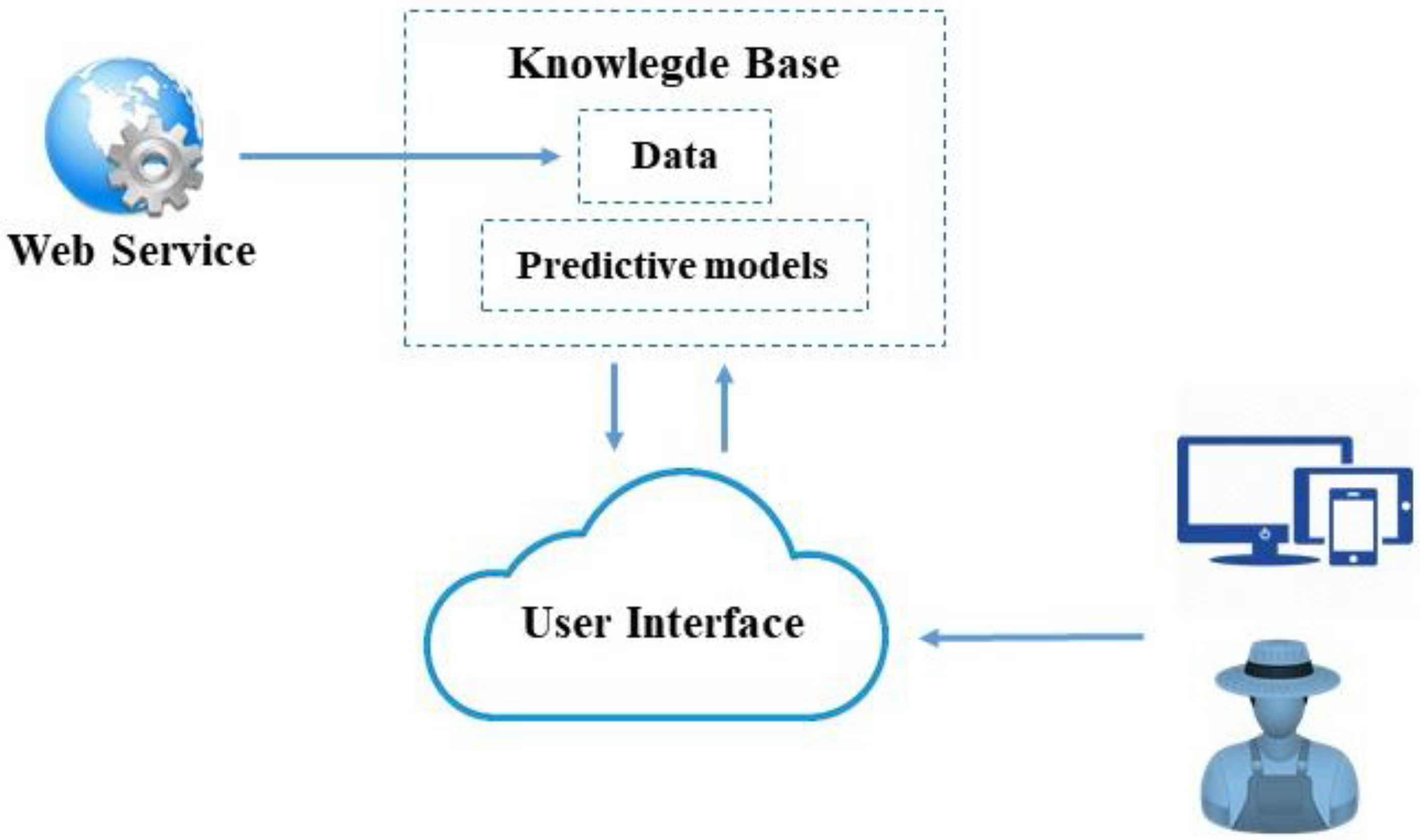
The data model for our system is quite basic; we just need two tables. The first table contains historical data including the amount of crop yield harvested in the olive grove on the farm under study each growing season, meteorological data, and environmental quality. The second table stores the results and input parameters of the prediction; both tables make the knowledge base of the system, Figure 4.

There are several tools to upload the data into the database. In this case, SQL-Loader has been used. It is a tool that allows us to read text files and transfer the data into the tables. Once the information was uploaded into the auxiliary tables, it was grouped by SQL querys following the framework criteria of the study.

2.4.2. Generating the Models with Oracle Data Mining

Oracle Data Miner is an extension to Oracle SQL Developer that allows data analysts to work directly with the data within the database, explore the data graphically, build and evaluate multiple data mining models, and more. The Oracle Data Miner workflow captures and documents the user’s analytical methodology and can be saved and shared with others to automate advanced analytical methodologies. It also allows the creation of predictive models that application developers can integrate into applications to automate the discovery and distribution of new business intelligence: predictions, patterns, and discoveries.

Once the data was stored, the models were generated with Oracle Data Mining. This was performed using the SQL Developer tool. First, we selected the source table and the type of model we wanted to generate, in our case, a regression. Then, we selected the algorithm to apply, and the system asked us to select the target attribute and the attributes that form part of the predictive model.

2.4.3. Development of the Application and System Learning

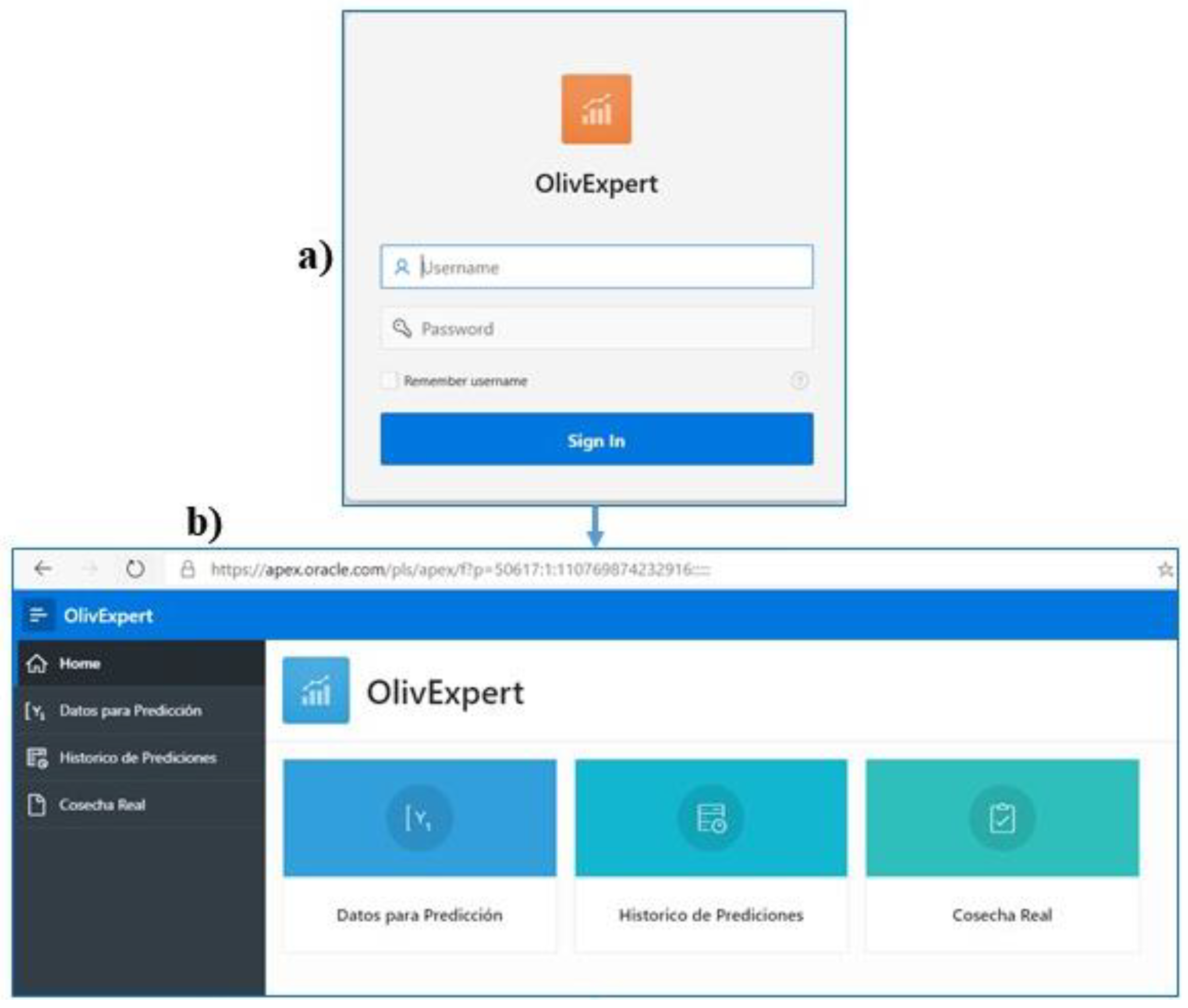
The second objective of this work is to integrate the prediction system into a useful application for the farmer or manager of the olive farm. As this is a user who is not an expert in Information and Communication Technologies, it is a priority that the system is implemented in a simple application with a user-friendly interface. Oracle Application Express (Oracle Apex) has been used for this purpose. It is an Oracle’s primary tool for developing Web applications with SQL and PL/SQL. Using a web browser, professional Web-based applications for desktop and mobile devices can be developed. 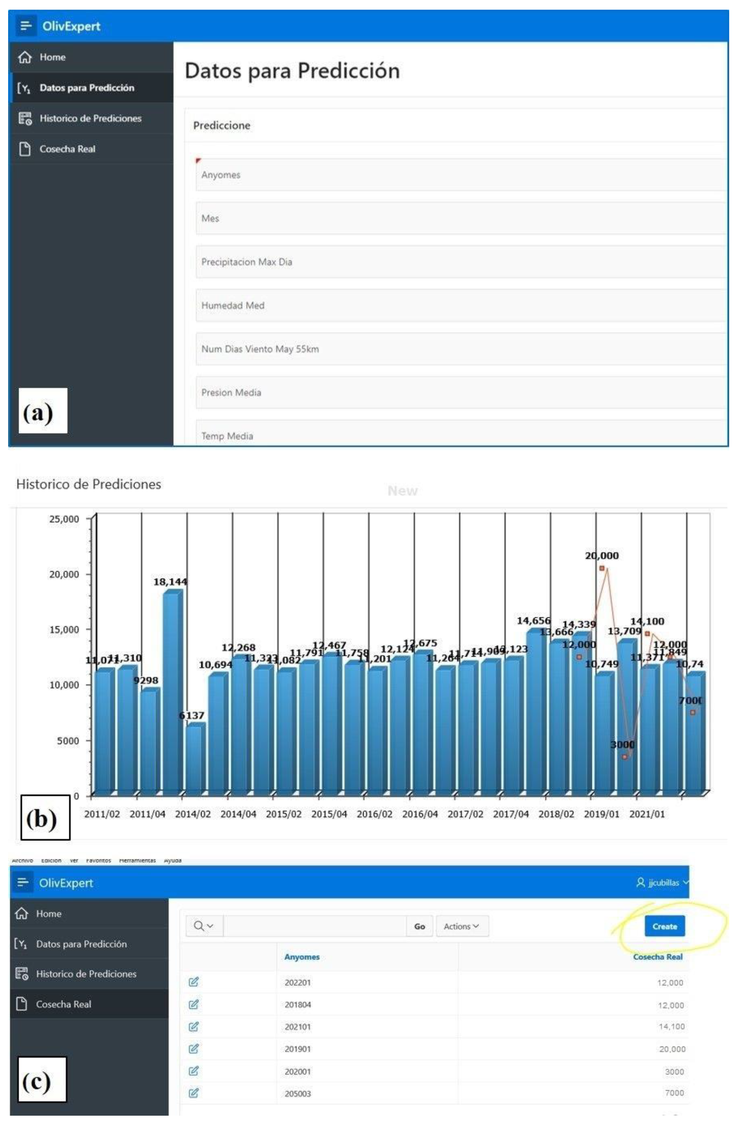In this study, the system has been mounted on Oracle’s Cloud, allowing it to be accessed from the Internet on the page https://apex.oracle.com/pls/apex/f?p=50617 (accesed on 20 February 2022). The system has the following functionalities:

9.

Log-in system. In order to access the system, user registration and authorization is required, Figure 5a.

10.

Main screen. There are 3 icons, Figure 5:

a

Prediction data. This accesses the screen where the user inserts the data to make a prediction. It opens a variable collection form. Figure 6a.

b

Historical Data. This allows us to visualize the result of all the predictions made by the system. It is possible to search for any prediction made by the system at any time in different formats (table, report, or graph), send it to anyone by mail, make groupings, etc. You can even make simulations from fictitious data. Figure 6b.

c

Real Yield Data. In this option, the user enters the real data on the amount of harvest harvested in that year. This data becomes part of the training data, so the system is learning through a continuous feedback process, Figure 6.

Finally, the screen showing the result of the web application was designed. To do this, the wizard provided by Oracle APEX was used and relied on the same results table. To improve the interface and help the manager, the application generates representative graphs of the stored data, such as the harvested data versus the prediction values for each year.

3. Results

3.1. Datasets Analysis and Data Cleaning

The idea is to use data from the first seven years to generate the model and the last one to analyze the quality of the prediction. The development of this data mining study includes the following phases: data loading, data cleaning, detection of anomalous data, generation of predictive models, and finally testing for validation. Firstly, a table was created in order to store the information extracted from the AEMET Web Services as well as the harvest quantity data supplied by the farmer. Previously loaded data in the database JSON files were converted to CSV using “|” as field delimiters. Once this conversion was carried out, they were loaded into the database. All the information was stored in a single table, denormalized.

Additionally, data were also analyzed with a one-class classification algorithm for the detection of anomalies. A one-class classifier develops a profile that generally describes a typical case in the training data. The profile deviation is identified as an anomaly. Outliers are sought in this study, such as unusual cases, because they fall outside the distribution considered normal for those data.

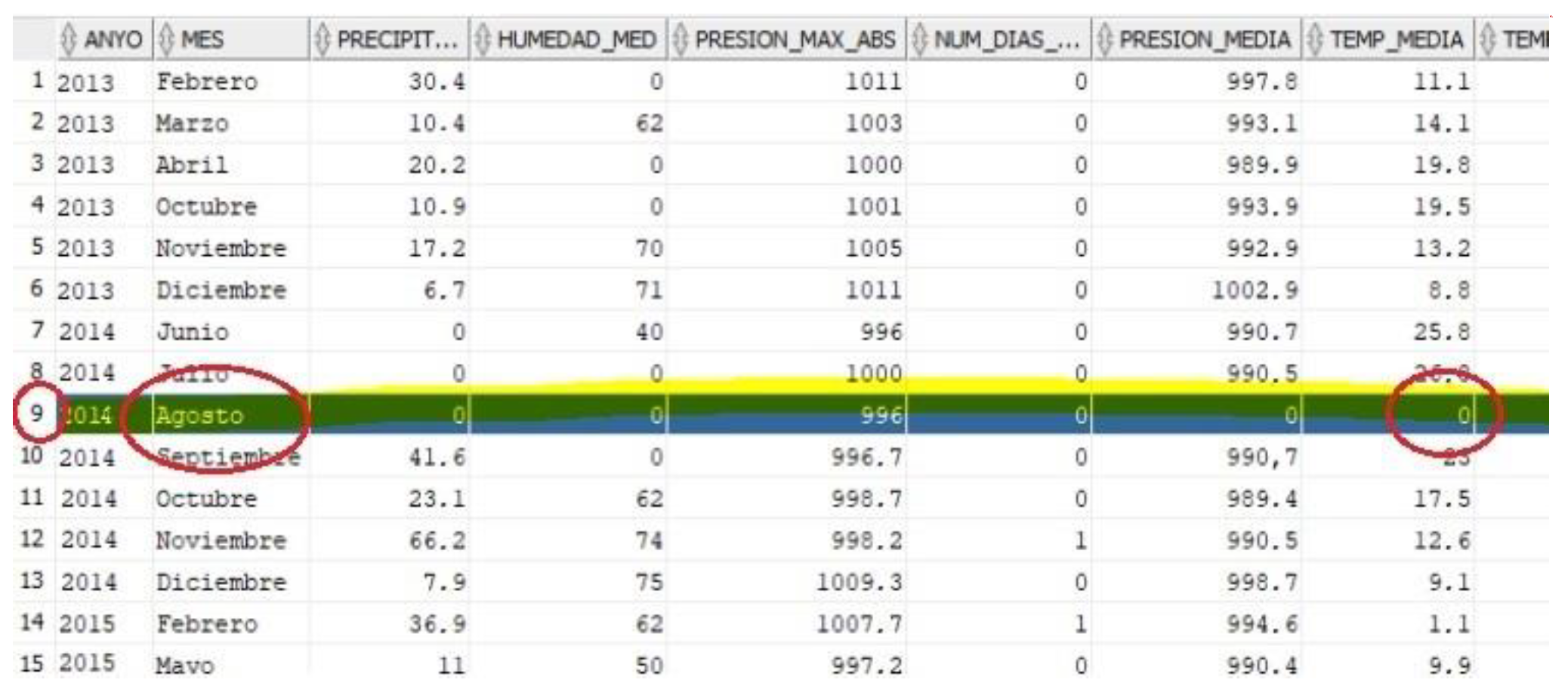
The algorithm shows the distribution of the data and marks with 0 abnormal data together with their probability. The results can be seen in

Table 3. Results of the one-class classification algorithm.

Anomaly Detection	Probability (%)
1	50.19
1	66.72
1	62.08
1	64.90
1	67.38
1	65.18
1	62.58
1	53.31
0	75.48
…	…

, in which record number 9 is marked as anomalous value with a probability of 75%.

The anomalous value detected was removed from the study. Figure 7 shows the values of this abnormal record, and indeed, it can be confirmed that August marks a maximum temperature of 0 degrees, minimum temperature of 0 degrees, etc. It is clear that it is an outlier (that is a mistake in the data), because in Jaen, the mean temperature in August is higher than 30 degrees. This review of the table could hardly have been carried out with the naked eye. This checking and filtering of variable values ensures that the data used as training data are quality data. Consequently, the final prediction errors are attributed to the adequacy of the model/equations and not to the parameters.

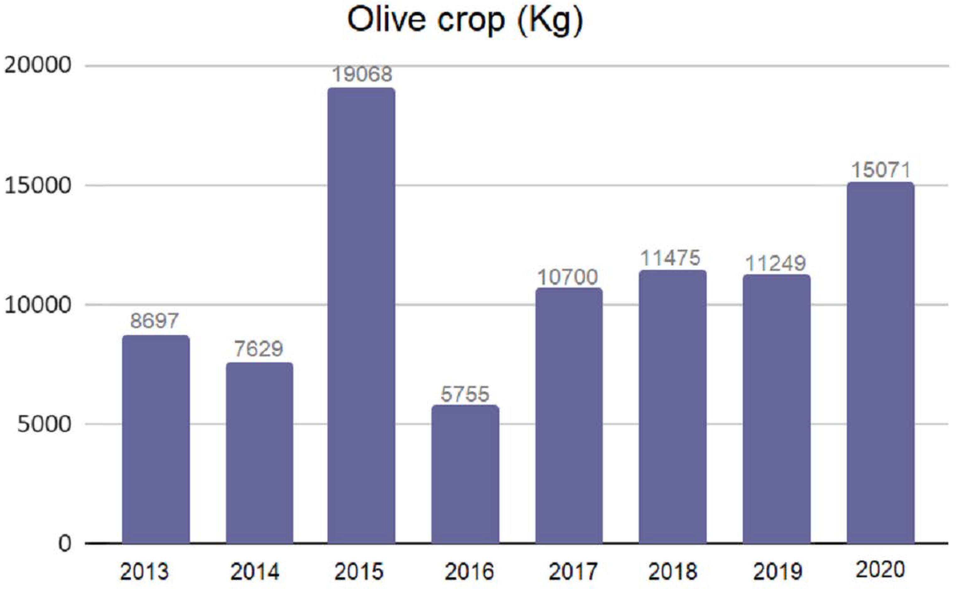
In addition to the analysis of the meteorological variable data, an analysis of the yield data was carried out. When analyzing the harvest quantity data for each year, Figure 8, it was observed that the maximum and minimum values correspond to two consecutive campaigns, those of 2015 and 2016, with values of more than 19,000 kg and around 5000 kg, respectively. This is a significant difference, more than 300%. At first it could be considered that this fact could negatively affect the model testing, since it presents a significant peak jump in the distribution of the yield data. However, if the 2015 data is excluded from the training data to generate the model when testing its prediction, the model validation will give good results, but for global model purposes there will be no training data with the 2015 crop. The same argument could be applied to the 2016 crop data, so it is to be expected that although the prediction of the 2015 and 2016 crop will not be reliable in the validation check, this does not imply a deficiency of the model. The reason is that this circumstance, in the final model, is mitigated by including all years as training data, i.e., from 2013 to 2020. In this sense, as the amount of training data increases, the model will be adjusted to the different casuistry of each year.

3.2. Variables Influencing Olive Crop Prediction

The next phase in the workflow of this study is to determine the level of influence of each variable on the target attribute, in this case, the crop harvested in each year. The Minimum Description Length algorithm (MDL) was applied. This algorithm returns a value of between −1 and 1. Values of 0 are returned for those cases which have no relationship. For this study, only those attributes with weight greater than 0 were considered, discarding those attributes with a 0 or negative value. Once the most suitable attributes for this study were selected, they were used to generate the predictive models.

Table 4. Ranking and weight assigned to each attribute.

Variable	Level of Influence on Target
Last year’s crop	0.793
np_300	0.436
nw_55	0.156
nt_00	0.152
np_100	0.132
p_mes	0.121
ti_max	0.111
p_max	0.092
ta_max	0.091
e	0.073
tm_mes	0.061
nt_30	0.053
w_med	0.042
tm_max	0.041
ts_min	0.031
tm_max	0.021
nt_00	0.019
q_med	0.015
hr	0.015
np_001	0.015
np_300	0.005
month	0.004
q_max	−0.756

shows the results of the algorithm execution. Here it can be confirmed the variables that have been included in the model are those that have a level of influence on the target attribute above zero; those with a negative influence value have been discarded. The attribute with the greatest influence is the harvest quantity of the previous year, last year’s crop. Then, the next variable in importance level is the number of days with rainfall greater than 30 L, np_300, followed by the number of days with wind of more than 55 km/h, nw_55. It is understood that this will affect pollination. It was also observed that the absolute maximum atmospheric pressure, q_max, data have a negative value and, therefore, is not related to the target attribute; this attribute was removed from the study.

3.3. Models and Validation

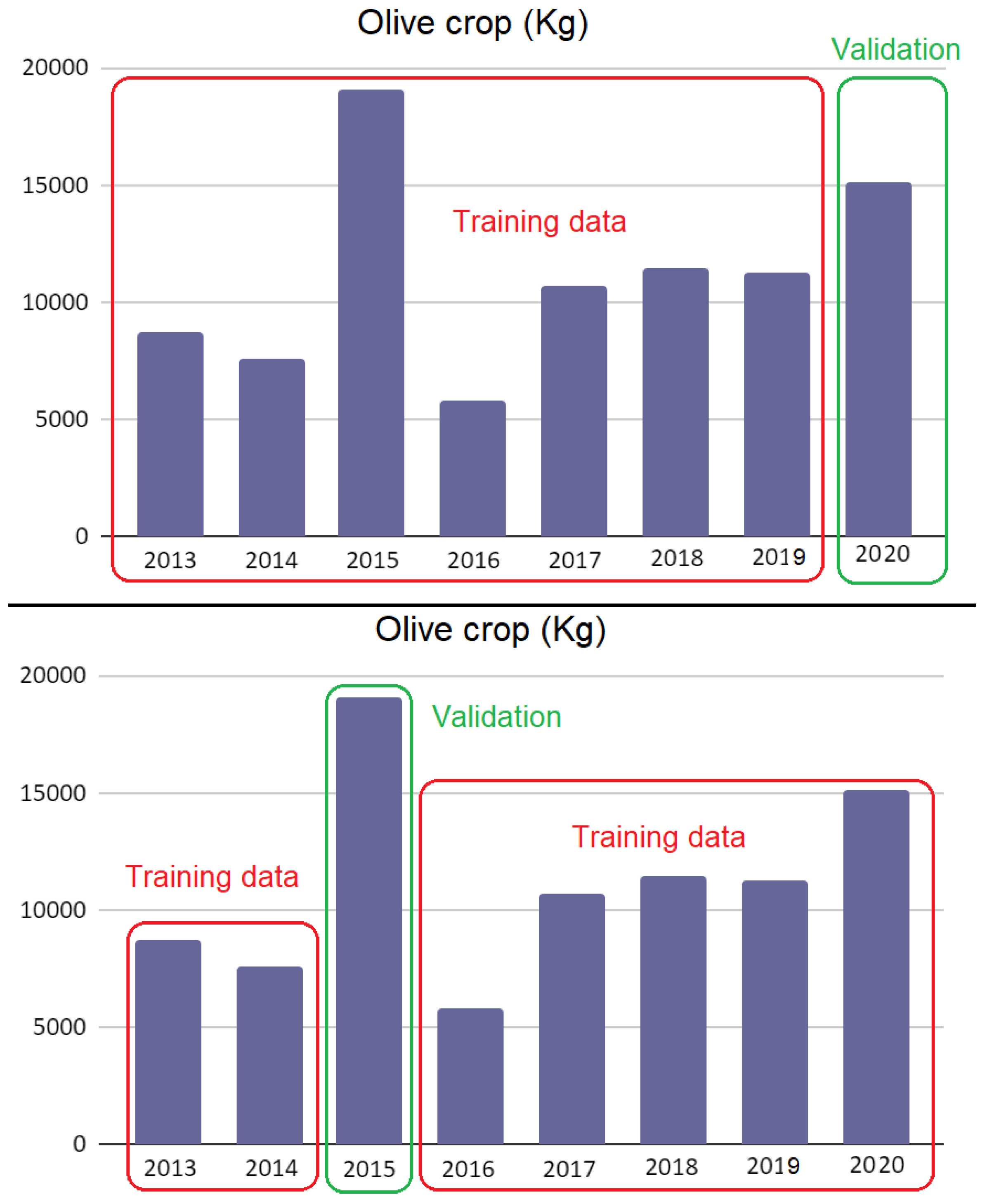
Once variables were selected and all information was available and normalized, the model was designed. The k-fold cross validation technique was used to evaluate results in statistical analyses [44]. The technique consisted of evaluating the quality of each year’s prediction by separating that year’s data from the training data used for the prediction. Particularly, for this research, it was used to check the reliability of the model in terms of harvest quantity prediction of a specific year, being this excluded in the generation of the model. As previously indicated, for this study, production data from 2013 to 2020 were used. Specifically, a predictive model was generated using data from seven years, and next, data from the eighth were used to evaluate the reliability of the model; that is, the prediction of the harvest of the eighth year was estimated and then it was compared with the actual crop data of that date.

There was no dependence between the training data and the prediction; therefore, another model will be generated with the data for the years 2013, 2014, 2015, 2016, 2017, 2018, and 2020, and its reliability will be tested in the 2019 crop prediction, and so on. In this way, the model can be tested against the actual production of several years, Figure 9. Finally, a final model will be generated including all years, that is, using all training data.

Another important consideration in the design of the model is the reliability of an early prediction of the crop during the harvesting year. As indicated in previous sections, the farmer must make decisions once the harvesting year has been completed, that is, from January to March, he has to make decisions regarding tilling the land, fertilizing it, pruning it, selling the oil obtained, etc. In this sense, in this study, since the meteorological data are grouped by months, a monthly prediction of harvest quantity is generated and then the quality of each prediction is assessed. Thus, for each year, 12 predictions were generated, one for each month, and the mean absolute error (MAE) of each prediction was calculated in order to determine how consistent the prediction was. The MAE is the average of all absolute errors, and it is calculated as shown in Equation (5), where n is the number of errors, Σ is the summation symbol which means “add them all up”, and |x_i − x| is the absolute errors.

$$\mathrm{MAE}=\frac{1}{n}{{\displaystyle \sum }}_{i=1}^n|x_i-x|$$

(5)

In this way, the farmer has a series of tools in addition to his own experience to make appropriate decisions about the management of his farm.

As the predictive model generation process has been designed, a cross validation is carried out. For this purpose, several models are generated, one for each year to be checked. A pure linear model is used from the GLM algorithm and other models applying SVM with Gaussian and Linear Kernel, respectively. Once the algorithms have been tested, the one that best suits the nature of the data is taken into account. Finally, the final model is generated using this algorithm, including as training data all the harvest years from 2013 to 2020.

In this first phase of results, the models generated for cross-validation are presented. A model is generated for each year to be tested. For example, to check the year 2020, training data included are from 2013 to 2019. Those for 2020 are not included; they are used to test the effectiveness of the model. In other models, we proceed in the same way, but checking the year 2017. The model training data are: 2013, 2014, 2015, 2016, 2018, 2019 and 2020, leaving 2017 out, as it is used for testing, and so on. Three different algorithms are used: a pure linear model such as GLM and others such as SVM with Gaussian and Linear Kernel.

The Oracle Data Mining tool is used in this research to provide information about the theoretical efficiency of each generated model, Figure 10. To analyze the effectiveness of each model, we analyzed the MAE, as seen in Equation (5) and also the root mean square error (RMSE), The latter is the standard deviation of the residuals, prediction errors. Residuals are a measure of how far from the regression line data values are. RMSE is a measure of how spread out these residuals are. In other words, it indicates how concentrated the data are around the line of best fit. In Equation (6), n is the number of values predicted.

$$RMSE=\sqrt{{{\displaystyle \sum }}_{i=1}^n\frac{{\left(Predicte{d}_i-Actua{l}_i\right)}^2}{n}}$$

(6)

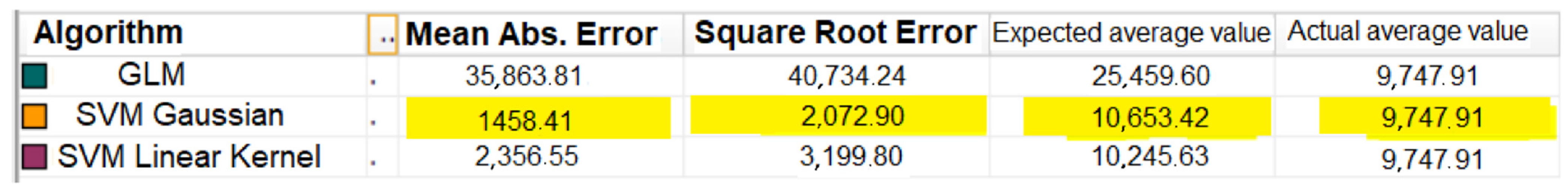
In the comparison of the three models, it is observed that the lowest errors, both for MAE and RMSE, are those obtained with the SVM model with Gaussian Kernel. Therefore, based on these data, the selection of this algorithm to generate the final model is justified. The real data for the year 2020 are used for the error comparison.

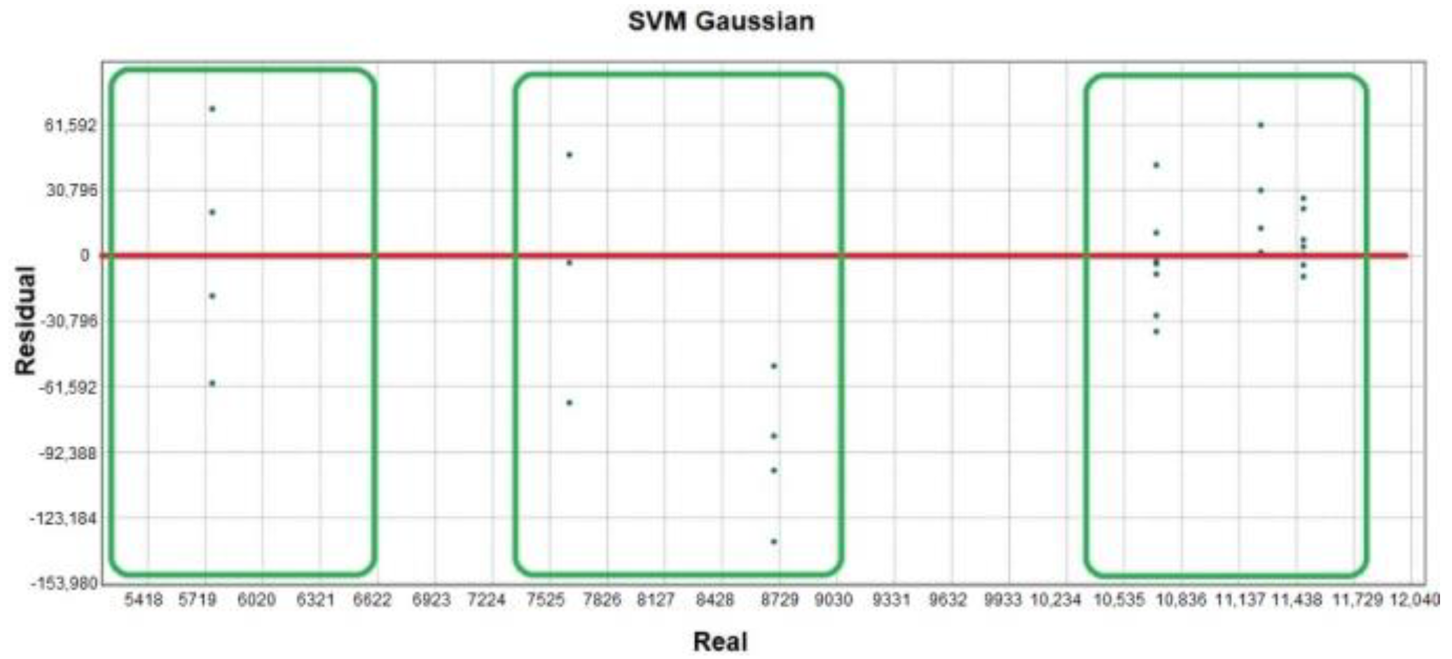
The residual plot is also analyzed to visualize graphically how the model fits the evolution of the data. Thus, it detects strange behaviors in individual data, Figure 11. Three large groups that are very far apart, whose values have an influence on the model can be detected. Although they are very distant from each other, they are not considered as outliers since the residuals are homogeneously located in the three groups. Analyzing the impact of the last year’s crop variable on the model, it can be confirmed that harvests can be basically classified into three types: low harvest, medium harvest, or high harvest.

As indicated in the introduction, the optimization of agricultural resources on an olive orchard requires the farmer to make appropriate decisions in advance. In this sense, resource management during the months of January or February is crucial, since there is still no indication of what the harvest will be that year. However, the contribution of this research focuses precisely on providing reliable data to the farmer also at an early stage of the agricultural year of the olive crop.

Table 5. Early prediction of crop data for each year (kg/ha).

Year	Month	Yield Data	Prediction	Relative Error
2020	January	4566.18	3815.97	16.43%
	February	4566.18	4275.08	6.38%
2019	January	3408.20	3592.49	5.41%
	February	3408.20	3806.77	11.69%
2018	January	3476.67	3141.15	9.65%
	February	3476.67	3478.94	6.52%
2017	January	32.42	3881.56	19.73%
	February	32.42	3763.93	16.10%
2016	January	1743.64	2481.55	42.32%
	February	1743.64	2588.64	48.46%
2015	January	5777.19	3511.67	39.00%
	February	5777.19	5760.12	29.54%
2014	January	2308.39	2310.70	10.03%
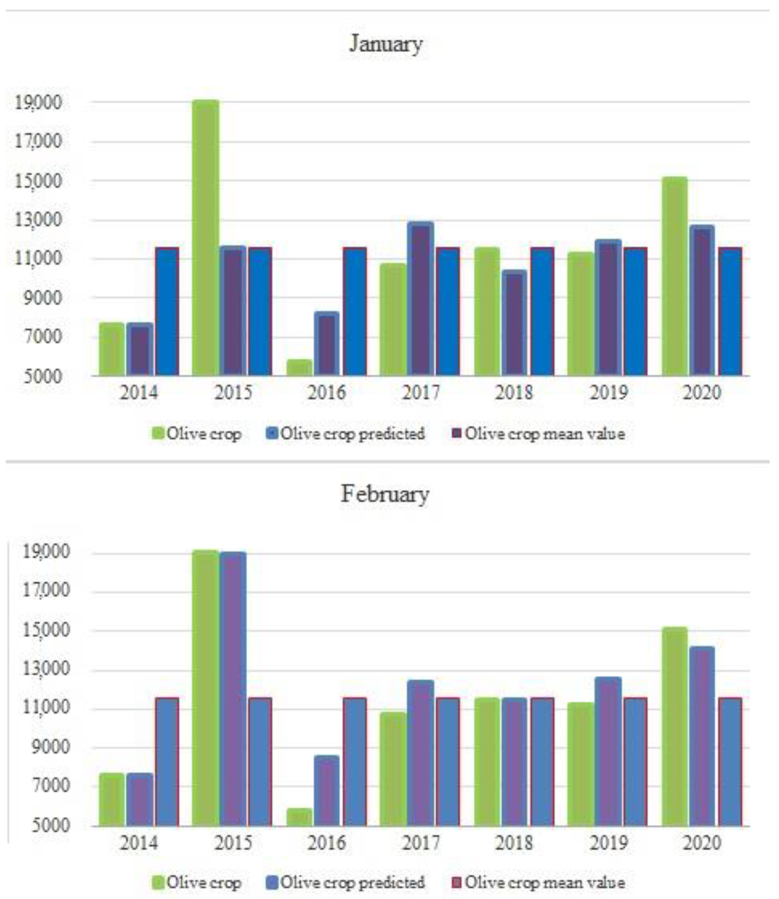
	February	2308.39	2310.08	7.32%

shows the model predictions for the months of January and February of all years. Note that the prediction for 2013 is not included. This year, being the first year, its data are used as training data, but the harvest cannot be predicted because data from the previous year are not available.

However, crop prediction errors for 2015 and 2016 are less encouraging. The latter range between 48% and 39%. In this regard, it is important to remember that the yield data for these two years correspond to the maximum and minimum values, respectively, of the total training data set. Therefore, these results are to be expected in the validation study since, in order to perform the cross-validation for the years 2015 and 2016, the data for each year are not included in the training data. For this reason, the model is overestimated, and these results come out. However, this is not a problem, since these extreme data are included in the final model, and in a similar situation the regression model would fit more accurately.

Traditionally, the farm manager usually makes decisions based on the average values of previous years, which, in the case of years with extraordinary circumstances, our predictive model would be able to provide extraordinary knowledge. In this sense, considering the crop variability between maximum and minimum is more than 331%, between 2015 and 2016, having an error of 48% in January, this prediction could be useful for the farmer. In fact, cross-validation of the prediction for the months of January and February, Figure 12, confirms that the crop prediction for these two years of extreme values is closer to the actual values than the naïve model, based on averaged values.

Once the algorithms have been tested, taking into account that the SVM algorithm with Linear Kernel is the one that best adapts to the nature of the data that influence the target attribute, the amount of harvest was generated, which includes as training data all the harvest years, from 2013 to 2020.

4. Discussion

An early crop yield prediction in the crop season, January-February, as resulted in previous sections, is key for the farmer to make important decisions, such as choosing the type of tillage on the farm, investment in fertilizers, irrigation, or even the marketing of the oil. These decisions are highly dependent on the crop forecast. Currently there is research oriented to the generation of predictive models; however, although they are very efficient, they are not useful for the case of olive orchards. The main reason is that these models are based on the analysis of pollination [16,21,22,23,24,25,26,27,28], which occurs very late in the crop year, between May and July. Moreover, in this period, the fruit is already visible on the olive tree, so the farmer, based on his knowledge of previous years, can already have a reliable idea about the harvest; therefore, it is a good and reliable prediction, but not very practical because the economic investment in ploughing and other work on the exploitation has already been made.

The contribution of this research is that based on historical olive crop harvested data and meteorological data such as temperature, rainfall, wind, etc., crop prediction models on February have been generated, with absolute errors of less than 17% in 70% of the years used for the training data. Similar results have been obtained by other authors, but in research related to early potato harvest prediction. In this work, regression models and yield data from seven previous years have also been used, obtaining a mean absolute error of around 15%, with the same validation method [45]. Taking into account that crop variation from one year to another can vary by more than 330%, these results can be considered satisfactory. In addition, due to the design of the study, the errors obtained are maximum errors, since training data were excluded for the validation tests; however, in the final model, the training data are composed of yield data from all years, which increases the robustness and efficiency of the predictive model.

As a particular case, in the years of maximum and minimum harvest, relative errors of around 40% have been obtained, Table 5. This is a large error compared to the rest of the years; however, it is an acceptable error considering that this error is not real and is overestimated. When removing, in the cross validation, data from the years of maximum and minimum harvest, there are no training data for these harvest extremes, hence such large differences between the estimated and real values. Even so, the model fits with a relatively low error, making an acceptable prediction for the margins of error typical of such an early prediction. However, as already mentioned, these values are included in the final model, thus allowing the model to be able to predict future extreme harvests under similar circumstances.

The study confirms that the main variable that most influences the prediction of harvest quantity is the previous year’s harvest. In this sense, and to demonstrate the sensitivity of the model to this variable, the harvest prediction for the growing seasons of 2015/16, 2016/17, and 2017/18 was generated by considering the actual harvest values of the previous year in the training data. The harvest data for the year before each season was then increased by 10%, and each of the three predictions was generated again. It should be noted that the rest of the variables were kept as the real values. The results can be seen in

Table 6. Comparison in yield data prediction (Kg) by changing the key parameter by 10%. Analysis for three selected growing seasons. (1) Prediction using real values for the key parameter and (2) prediction using the key parameter value modified by 10%.

Growing Season	Yield Data Current Season	Real Yield Data Previous Season	Prediction Current Season (1)	Changed Yield Data Previous Season	Prediction Current Season (2)
2015/16	11,475	10,700	10,367.58	9630	11,033.24
2016/17	11,249	11,475	12,564.51	10,327.5	12,664.51
2017/18	15,071	11,249	14,110.19	10,124.1	14,412.36

. It can be seen that decreasing the harvest of the previous year by 10% has a direct effect on the prediction; in such a case, the lower the harvest of the previous year, the higher the prediction.

In this harvest prediction research, harvest data and meteorological values have been used. In fact, the Discussion of this paper focuses on these two variables as key parameters. The reason is that, as already developed in the methodology section, the MDL algorithm provided us the level of influence of each variable on the target attribute, with the amount of harvest from the previous season and rainfall being the most influential. However, in other works [46], remote sensing data have also been used. However, in this study, it was found that the estimation results change depending on different agricultural zones and temporal training settings. Nevertheless, factors influencing crop production used to be the same, the greatest weight attributed to environmental factors such as crop variety, soil type and surface cover or topography, etc.

The analysis of the influence of the variables studied on the early harvest prediction has been carried out using the MDL algorithm. The results obtained are in line with the works [47,48], which state that years of very good olive yields alternate with other in which very few kilograms of olives are harvested per tree. This alternation is not due to climatic factors, but to the fact that the high yields of the productive years interfere with the vegetative development of the tree or exhaust its reserves, and therefore, it will need time to recover and accumulate the lost resources again. This has been confirmed in our study by analyzing the variables that influence the amount of harvest, the target attribute. The MDL algorithm statistically quantifies that the most influential variable is the amount of harvest from the previous year, Table 4. The analysis of the influence of the variables studied on the early harvest prediction has been carried out using the MDL algorithm. The results obtained are in line with the works [47,49], which state that years of very good olive yields alternate with others in which very few kilograms of olives are harvested per tree. This alternation is not due to climatic factors, but to the fact that the high yields of the productive years interfere with the vegetative development of the tree or exhaust its reserves and, therefore, it will need time to recover and accumulate the lost resources again. This has been confirmed in our study by analyzing the variables that influence the amount of harvest, the target attribute. The MDL algorithm statistically quantifies that the most influential variable is the amount of harvest from the previous year, Table 4. In addition, the argument of alternation between productive crop years and crop-shortage years is also corroborated in this study from the residue analysis in Figure 11. Here, we can see how the harvest quantity data are grouped into three clearly differentiated classes: low harvest, medium harvest, or high harvest.

Secondly, another key variable in crop production is the amount of rainfall, especially that accumulated at certain times of the year. This has been confirmed by several authors [49,50,51], whose results showed in these works identify the highest production coincided with increased rainfall, namely in two consecutive months, during August and December. It was concluded that the impact of rainfall on olive production depends on the intensity and monthly distribution of rainfall. In this sense, our work identifies the variable "np_300" as the second most influential variable on the target attribute. This variable identifies the number of days of precipitation greater than or equal to 30 mm in the month/year, which coincides with the importance of the accumulated rainfall factor identified by the aforementioned authors.

The results obtained with respect to prediction reflect that of the three predictive algorithms used; the one that best fits the objective of this research is the SVM algorithm with Gaussian Kernel. This indicates that there is no linear relationship between the variables and the target attribute. The algorithm distributes the data in a Gaussian bell-shaped hyperplane in such a way that a plane of separation is established between the data, Figure 1. In this study, the following Gaussian Kernel configuration has been used in the SVM algorithm:

• Kernel Cache Size specifies the cache size (in bytes), which is used to store the kernels computed during the build operation. As expected, larger cache sizes generally result in faster builds. In our case, it has been configured with the value of 50 MB.
• Convergence tolerance specifies the tolerance value allowed for the generation of the model before completion. The value must be between 0 and 1. The value configured in our case was 0.001. Higher values tend to result in faster generations but less accurate models. In our study we have aimed for a value very close to 0 to ensure maximum accuracy without penalizing computational time.
• Standard deviation allows us to specify the standard deviation parameter that the Gaussian kernel uses. This parameter affects the trade-off between the complexity of the model and the ability to generalize to other data sets (overfitting and underfitting of the data). Larger standard deviation values favor under-fitting. We have left this parameter with the default setting. With this setting, the system has automatically estimated this parameter from the training data.
• Epsilon. Specifies the value of the error interval allowed in the generation of models not sensitive to epsilon. In other words, it distinguishes small errors (which are ignored) from large errors (which are not ignored). The value must be between 0 and 1. As with the previous parameter, the default setting has been used, so that it has been calculated by the system based on the training data.
• Complexity factor. Allows the determination of the complexity factor that balances model error (measured with respect to the training data) and model complexity in order to avoid over-fitting or under-fitting of the data. Higher values provide a higher penalty to errors, which means a higher risk of over-fitting the data. Smaller values provide a smaller penalty to errors and may lead to under-fitting. In our study, this value has been set as automatic and the system has determined it based on the training data.
• The normalization method specifies the method used for the continuous input and the target attribute. Z-scores, Min-Max, or None can be selected. Oracle performs the normalization automatically if none is specified. In our case, it has been left unselected.
• Active learning provides a method for handling large generated sets. With active learning, the algorithm creates an initial model based on a small sample before applying it to the entire training data set and then updates the sample and model incrementally based on the results. This cycle is repeated until the model converges on the training data or until the maximum number of allowed support vectors is reached. In our case, to speed up the calculations, this parameter has been activated.

Given the specific configuration of the parameters used in the algorithm, it could be concluded that the model generated is only valid for the case of the farm studied. For this reason, and in order to check its effectiveness at other scales, our model was tested on a much larger area. The statistical model has been applied to another crop prediction in Spain, but this is a much larger farm extension, the joint prediction at the level of all the farms belonging to the same municipal district, Lahiguera (Jaén, Spain). This includes 50% of traditional rainfed olive groves and the other 50% of irrigated olive groves. Harvest prediction was generated for the 2020/21 and 2021/22 seasons. Our model was trained with data from the 2013/14 seasons up to the 2021/22 season. As in our study, we removed the year to be predicted from the model, Table 5. The meteorological data were obtained from two stations located within the boundary of Lahiguera, and the arithmetic means of the climatic data were used. The predictions obtained had similar relative error to those of our case study,

Table 7. Early prediction of crop data for Lahiguera district (Kg).

Growing Season	Yield Data	Prediction	Relative Error
2020/21	15,349,191.85	15,899,198.74	3.58%
2021/22	14,823,594.35	16,367,993.56	10.41%

.

In summary, despite the local character of the study, the results are in line with larger scale studies and with the results of other authors elsewhere, which is another way of validating our methodology. It is also an endorsement to improve our predictive model by adding more data and more farms to our training data.

5. Conclusions

All development and generation of the predictive models were performed under the cloud application without the user being aware of it. The farmer or manager using the application only selected the prediction they needed to see. They could also export the information in the desired format or simply visualize a graphical representation of the results. The application is, therefore, a powerful tool that is very accessible and very useful for decision making.

The conclusions of this study respond to the case of a type of olive grove with specific characteristics, an unirrigated olive grove where traditional tillage is practiced. Future lines of work include the application of these models in other farms with similar characteristics and in others where a different type of tillage is practiced. It also remains to be seen how these models would respond in an irrigated olive grove or in other types of olive groves, such as the growing intensive and super-intensive olive groves, where the yield data are very different from those dealt with in this study. However, the working methodology and implementation in the web application is designed. Adaptation to other crop types would be achieved by following the same workflow and adapting the predictive models according to the influence of weather data and harvested crop quantity data.