Identification of Buffalo Breeds Using Self-Activated-Based Improved Convolutional Neural Networks

Abstract

The livestock of Pakistan includes different animal breeds utilized for milk farming and exporting worldwide. Buffalo have a high milk production rate, and Pakistan is the third-largest milk-producing country, and its production is increasing over time. Hence, it is essential to recognize the best Buffalo breed for a high milk- and meat yield to meet the world’s demands and breed production. Pakistan has the second-largest number of buffalos among countries worldwide, where the Neli-Ravi breed is the most common. The extensive demand for Neli and Ravi breeds resulted in the new cross-breed “Neli-Ravi” in the 1960s. Identifying and segregating the Neli-Ravi breed from other buffalo breeds is the most crucial concern for Pakistan’s dairy-production centers. Therefore, the automatic detection and classification of buffalo breeds are required. In this research, a computer-vision-based recognition framework is proposed to identify and classify the Neli-Ravi breed from other buffalo breeds. The proposed framework employs self-activated-based improved convolutional neural networks (CNN) combined with self-transfer learning. Moreover, feature maps extracted from CNN are further transferred to obtain rich feature vectors. Different machine learning (Ml) classifiers are adopted to classify the feature vectors. The proposed framework is evaluated on two buffalo breeds, namely, Neli-Ravi and Khundi, and one additional target class contains different buffalo breeds collectively called Mix. The proposed research achieves a maximum of 93% accuracy using SVM and more than 85% accuracy employing recent variants.

1. Introduction

The livestock of Pakistan includes goats, sheep, buffalos, cattle, and their variants. They have been used for milk, meat, wool, and hidden purposes. Rearing animals for milk and meat has always been a desirable task for our farmers [1]. However, lots of aspects of red meat are still to be illuminated, and there is a lot more to do in that sector; on the other hand, the milk sector of Pakistan is prosperous so far, and the need of the hour is to sustain this opulence and success [2]. According to the IFCN (international farms comparison network) report, Pakistan is the third-largest milk-producing country globally, and the figures are expected to mount in upcoming years [3]. Interestingly, Pakistan’s buffalos carry much of this burden as they constitute about 65% of total milk production in the entire country. Buffalos are the most widely used animal in South Asia, especially in Pakistan; Buffalo have been bred here for a long time, and Pakistan is fortunately rich in many world-class breeds of buffalo, such as Nili Ravi and Kundi [3].

Before the late nineties, a revolution occurred in Pakistan’s milk sector before almost 60% of animals were kept by rural people in small units. The grazing fulfilled the feed requirements and other green fodder [3]. In the last two decades, the dairy sector of Pakistan has witnessed rapid growth; lots of dairy farms have been established, and especially Kundi is a vital player [4]. Worldwide, there is a dearth of buffalos; previously, the developed world has primarily considered cattle as a principal source for getting milk requirements. The USA’s milk industry relies chiefly on dairy cattle, but now it is moving forward toward the utilization of Buffalo milk [5]. There are many reasons behind this shift, such as the low percentage of fat in cattle milk (buffalos have twice as much as cattle), its low viscosity (buffalo milk is much more viscous, thick, and creamy than that of cattle), and the inability of it to be rendered into some refining kind of cheese such as Mozzarella cheese and some varieties of Cheddar cheese, etc. To manufacture these from cattle milk, millions of dollars have been invested, but the results have been negative [6].

These buffalo breeds tolerate wide variations in fodder supply, feed quality, and adaptation to low-input monitoring systems. Their home track is in central Punjab’s canal-irrigated areas, where they are fed plenty of green fodder [7]. They produce much less milk in their home tract despite their capacity, which may be due to (1) a long calving interval, (2) silent heat, (3) late maturity, and (4) a lack of attention paid to the past to improvement by selection and progeny testing [7].

The classification of native buffalo breeds has traditionally been based on morphological differences, but regional variations are insufficient to distinguish breeds closely related [8]. For their effective and meaningful improvement and conservation, the detailed characterization and evaluation of differences among these breeds using modern technology tools is required.

The technological developments in the field of artificial intelligence (AI) [9], blockchain [10], IoT [11], cloud technologies [12], and data science [13] are going to transform the practice of traditional dairy farming into smart dairy farming. The latest challenge in dairy farming, which is in focus and an essential aspect of dairy farming, is to achieve animal health and welfare at the best possible standards, keeping in mind the high-performance potential of animals [14]. It is necessary for animal sciences to meet these challenges faced by the farmer’s introduction of technological advancement.

Artificial neural networks (ANNs) are one of the advanced computing methods used mainly for classification and prediction [15]. ANN is a multi-layer connected neural network that looks like a web. The basic ANN unit consists of an input, a hidden layer, and an output layer. Each layer has neurons or nodes, which are interconnected to each other in the next layer. Each node in the hidden layer has some weight and bias values. ANN is a nonlinear technique that can take any input. Some of the advantages of ANN include its ability to learn and model nonlinear and complex associations between inputs and outputs, as well as its ability to generalize as it can derive unperceived connections after learning from the primary inputs and their correlation with the outputs, making the model capable of generalizing and predicting undiscovered data [16].

Pakistan is the world’s second-most buffalo-populated country, accounting for 16.83% of the global buffalo population, with Nili-Ravi constituting the majority [17]. Due to extensive crossbreeding, the Nili and Ravi breeds have been combined into a single Nili-Ravi since the 1960s [18]. Compared to native breeds, this single Nili-Ravi is now considered the best-performing breed for meat and milk production. However, the differentiation between the Nili-Ravi breed and other native breeds is complex, and only experts can identify it. Visual feature-based classification is an exciting research topic with emerging AI-based techniques. The visual features include the shape of the head, horns, texture, and color, and the formation of the udder, foot, and tail [18].

Correct identification of the Nili-Ravi breed will help improve the number of quality animals, ultimately helping to elevate poverty in rural areas of Punjab, where most of the house expenses are met by selling buffalo milk. Using morphological markers and visual features to identify animals remains an expensive and time-consuming manual task by researchers. As a result, we demonstrate that a deep convolutional neural network can detect different breeds.

1.1. Objectives

The objective of this study is to propose a computer-vision-based recognition system for the identification and classification of Neli-Ravi buffalo breeds from other buffalo breeds. The proposed framework used self-activated-based enhanced CNN coupled with self-transfer learning. Information-oriented feature vectors were obtained by transferring feature maps and then classified using machine learning-based classifiers. The proposed method was tested on Neli-Ravi, Khundi, and Mix (a group of several breeds).

1.2. Related Work

As per our knowledge, no work has been done so far to segregate the Neli-Ravi breed from other buffalo breeds using machine learning and deep learning. The morphological features of Nili-Ravi buffalo are given with details in

Table 1. Morphological features of Nili-Ravi buffalo.

Sr #	Characters	Description	Image
1	Marking	White markings are often found on hind legs, fore legs, white spots on forehead, muzzle, and white switch on tail (30–40%)
2	Eye	Eyes are prominent, especially in the females. They are usually walled eyes (73.5%).
3	Body color	The color is black but brown color is not uncommon (10–15 percent).
4	Horns	Horns are short, broad at the base, and closely curled behind the base. A few animals (1–2 percent) have loose hanging horns.
5	Tail	The tail is well set on, broad at the base, and tapering at the ends at the fetlock or just below it in a big tuft of hair, which may hand on the ground with a white switch.
6	Body	Nili-Ravi buffalos are large size and have deep and low-set frames (massive and wedge shaped).
7	Head	The head is long, convex in the upper third but with a depression between the orbits. It shows good depth from the angle of the jaw to the base of the horns.
8	Neck	The neck is long and thin in females, while it is thick and powerful in the male. There is no dewlap, and the umbilical fold is small.
9	Udder	The teats are long, even squarely placed.

.

The authors previously contributed in [19], which included establishing an experimental image processing framework on a sheep farm, creating a database containing 1642 sheep images of four breeds recorded on a farm and labeled by an expert with their breed, and training a sheep breed classifier using computer vision and machine learning to obtain an overall precision of 95.8% with 1.7 mean difference. Their method may help sheep farmers distinguish between breeds efficiently, allowing for more accurate meat yield estimation and cost control.

The authors in [20] presented a deep-learning-based method for identifying individual cattle based on their predominant muzzle point image sequence features, which tackles the issue of missing or switched livestock and false insurance claims. They developed a set of muzzle-point images that were not publicly accessible. They also used a deep-learning-based CNN to extract meaningful shape information and visualize a cattle’s muzzle point picture. The derived function of muzzle point images is encoded using the stacked denoising auto-encoder technique.

The classification of horse breeds in natural scene images is addressed in [21]. The author collected a data set by exploring the internet. The dataset includes 1693 photos of six different horse breeds. For the classification and identification of horse breeds, deep learning techniques, specifically, CNNs, were used. The proposed dataset is used to train and fine-tune well-known deep CNN architectures pre-trained on the ImageNet dataset. As pre-trained CNN classifiers, VGG architectures with 16 and 19 layers, InceptionV3, ResNet50, and Xception, are used. The average classification accuracy of ResNet50 was 95.90%.

In the other study [22], the authors tried to classify six distinct goat breeds using mixed-breed goat photos. The images of goat breeds were taken at various recorded goat herds in India. Without causing discomfort to the livestock, nearly 2000 digital images of individual goats were collected in limited and unregulated conditions. For the efficient recognition and localization of goat breeds, a pre-trained deep-learning-based object-detection model called Faster R-CNN was fine-tuned using transfer-learning on the acquired images. The fine-tuned model can locate the goat and identify its breed in the image. The model was assessed using the Pascal VOC object-detection assessment metrics.

The authors compare various deep learning models and propose an Android application [23] that uses a smartphone camera to determine a given cat’s position and breed. The finalized model’s accuracy rate was 81.74%. Another research [24] aims to propose an AI-driven system for fish species identification based on the CNN framework. The proposed CNN architecture has 32 deep layers, each very deep, to extract useful and distinguishing features from the image. The VGGNet architecture is subjected to deep supervision to improve classification efficiency by incorporating various convolutional layers into each level’s training. They built the Fish-Pak dataset to test the performance of the proposed 32-layer CNN architecture.

The authors used deep learning models [25] to assess the absolute maximum accuracy in detecting the Canchim breed species, which is virtually identical to the Nelore breed. They also mapped the optimal ground sample distance (GSD) for detecting the Canchim breed. There were 1853 UAV images with 8629 animal samples in the experiments, and 15 different CNN architectures were tested. A total of 900 models were trained (2 datasets, 10 spatial resolutions, K-fold cross-validation, and 15 CNN architectures), allowing for a thorough examination of the factors that influence cattle detection using aerial images captured by UAVs. Several CNN architectures were found to be robust enough to accurately detect animals in aerial images even under less-than-ideal conditions, suggesting the feasibility of using UAVs for cattle monitoring.

Another study [26] suggested using CNN to develop a recognition system for the Pantaneira cattle breed. The researchers examined 51 animals from the Aquidauana Pantaneira cattle center (NUBOPAN). The area is situated in Brazil’s Midwest area. Four surveillance cameras were mounted on the walls and took 27,849 photographs of the Pantaneira cattle breed from multiple distances and locations.

2. Materials and Methods

Deep-learning-based identification and recognition approaches are widely used in medical, natural, animal, and many other fields. The deep convolutional network inspires researchers to identify and classify different instances based on the visual features [24,27]. The proposed research offers a self-activated CNN for the identification of buffalos breeds. The proposed CNN contains a 23-layer architecture with 5 blocks of convolution, batch normalization, reLU, and a max-pooling layer. Feature vectors extracted from CNN layers without transfer learning and self-activation reach up to 77.61% validation accuracy. However, applying transfer learning from the fully connected layer of the proposed CNN tends to increase the overall performance. All of the extracted feature vectors are employed for classification using classical ML classifiers with various test and train ratios such as 50–50, 60–40, and 70–30. The K-fold cross-validation techniques with 5 and 10 folds are also used to validate different ML classifiers’ performance. 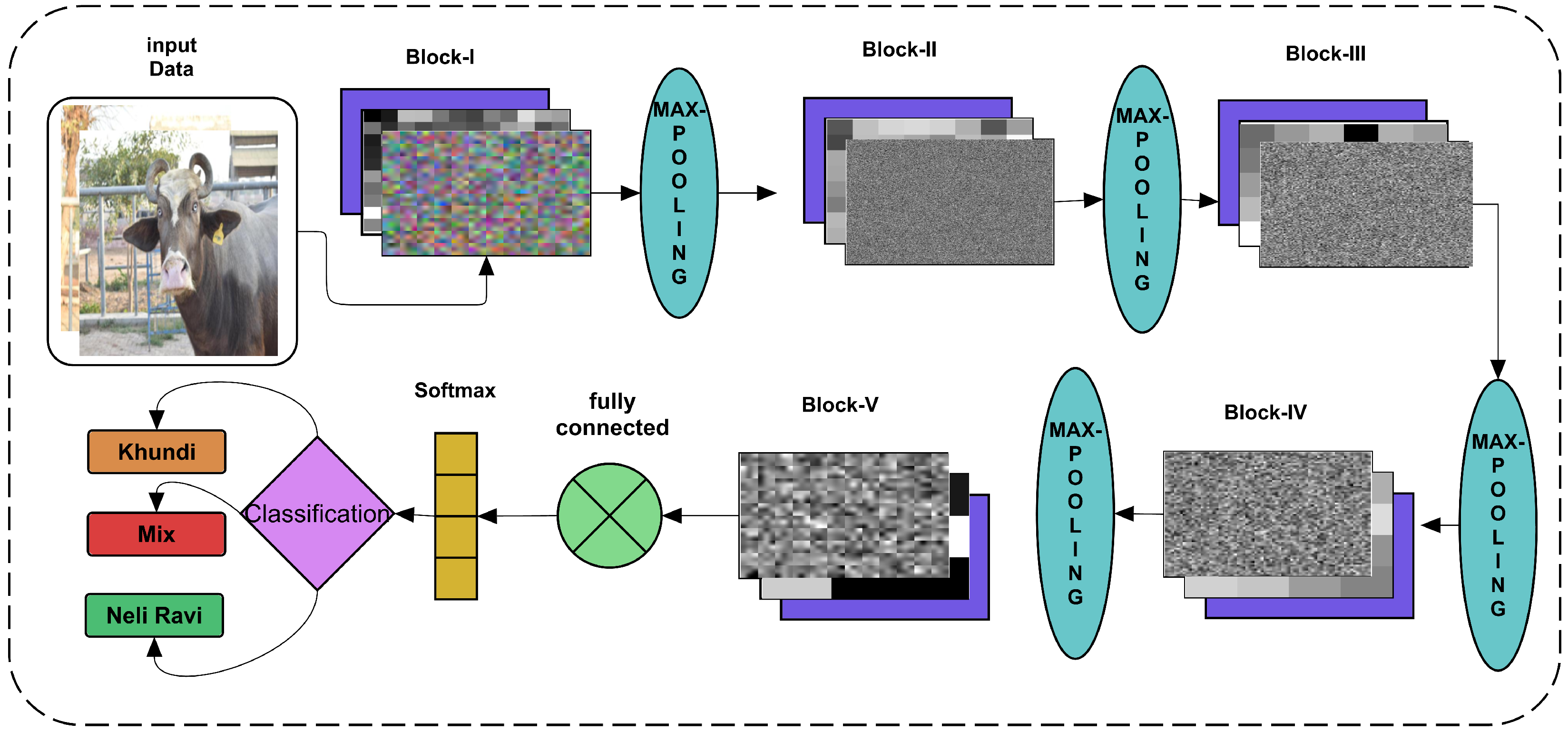The primary steps adopted in the proposed research are shown in Figure 1.

Figure 1 determines that the input data are augmented with rotation, clipping, and the pixel range. The augmented data are further transmitted to the proposed CNN to classify buffalos breeds. To extract the rich feature vectors, we applied transfer learning to the 21st layer of CNN, which splits into various ratios to classify the breeds.

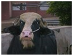
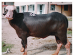
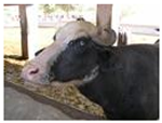
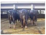
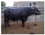
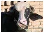
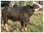
2.1. Data-Set Description

We collected data sets from Buffalo research center Pakistan. The acquired data-set is publically available at the data-set repository called Mendeley [28]. We normalized and preprocessed the data, including all class labels for self-activated CNN training. The size of the data set and details are shown in

Table 2. Data-set description.

Category	Frequency
Khundi	150
Mix	154
Neli-Ravi	146
Total	450
Format	JPG
Dimension	256 × 256 × 3

.

Table 2 has shown three categories of used data-set in the proposed research. The three classes include Khundi, Mix, and Neli-Ravi. All images’ dimensions and formats are kept the same as given, 256 × 256 × 3, and JPG, respectively. However, data are primarily augmented before training and testing to avoid over-fitting and other deep learning issues.

2.2. Data Augmentation

The data augmentation is performed using various augmentation techniques. The bounding points of images are being transformed using reflection in the X and Y direction at random locations. The X and Y transformation specifies that the image has left, right, up, and down reflections. The random X, Y translation is set to [−4, 4]. It defines the random translation in X and Y dimensions with a specific range of pixel intensities on the image. The used pixel range is −4 to 4. Moreover, random cropping is applied, which performs a specific bitwise hide and seek operation, including cut-out and random erasing on the given image. The data samples are shown in Figure 2.

2.3. Proposed CNN

The self-activated CNN architecture principally depends upon 23 layers containing five convolutional blocks with a different number of filters and sizes. The first layer is an image ($img[r,c]$) input layer having 256 × 256 × 3 input size of each given image instance. The 2nd layer is a convolutional layer with half the image size as several filters with a 3 × 3 kernel size. The padding and stride taken as one mean the sliding over the pixel to pixel for a given image are one so that each 3 × 3 kernel evolves on the whole image. The 2D convolutional computations are calculated as shown in Equations (2) and (3) by getting input from Equation (1) [29].

$$imputimage=I=img[r,c]$$

(1)

$$kernel=\left(\begin{array}{c}kernel\left(1,1\right)kernel\left(1,2\right)kernel\left(1,3\right)\\ kernel\left(2,1\right)kernel\left(2,2\right)kernel\left(2,3\right)\\ kernel\left(3,1\right)kernel\left(3,2\right)kernel(3,3)\end{array}\right)$$

(2)

$$y(i,j)=\sum _{i=-1}^1\sum _{j=-1}^1\mathrm{I}(x+i,y+j)\ast kernel(2+i,2+j)$$

(3)

The Equation (2) represents the general kernel mask of 3 × 3, which later multiplies with the input image, where i and j represent the rows and columns; at the end of convolve operation, the output matrix is calculating in $y(i,j)$.

Each batch normalization layer is used in all convolutional blocks, where batch normalization is used for input normalization by calculating the variance ${{\sigma }_B}^2$ and mean ${\mu }_B$ for each colour channel.

$$g_{x_i}={(x}_i-{\mu }_B)/\sqrt{{{\sigma }_B}^2+ϵ}$$

(4)

$g_{x_i}$ in Equation (4) is calculating the activated normalization, which is anticipated by using the division of difference between input $x_i$ and mean ${\mu }_B$ with the square root of the sum of squared variance ${{\sigma }_B}^2$ and constant value. The constant value invariance is added to stable the minimal variance value. The re-consideration of this activation is taken as $g_{y_i}$; the zero mean and variance with the unit value are essential to scaling. The scaling is shown in Equation (5).

$$g_{y_i}=\gamma g_{x_i}+\beta$$

(5)

In Equation (5), the learnable factors $\gamma$ and $\beta$ add to scale the activated output. The multiplication will shift the previous activated output into a new value with learnable parameters.

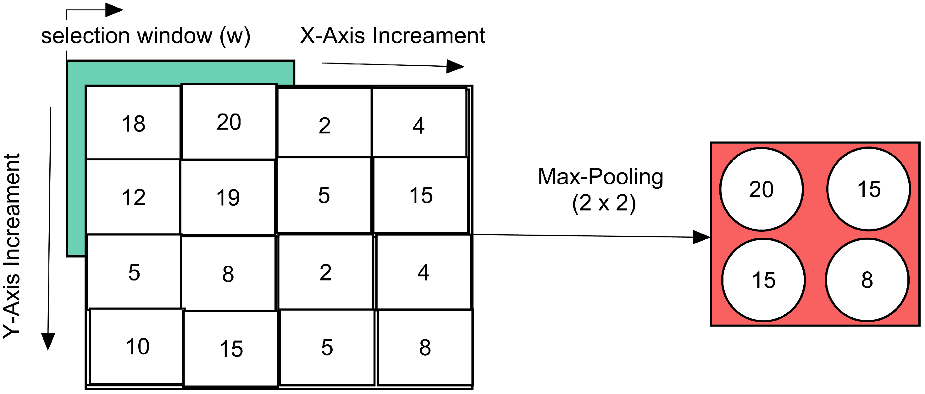
The max-pooling layer is down-sampling the given upper inputs into higher intensity values. The max-pooling for each convolve block is computed in Figure 3.

For iteration over the 2D matrix of an image, the input image selected the window, as explained in Equation (6).

$$w=I_{{selected}_{2x2}}$$

(6)

The max-values from each incremented window ‘w’ are taken firstly from the left to right of the image, and then the next row is started; in this way, the y-direction increment starts, and lastly, a max-pooled downloaded max-window is gathered for each activated input of upper layer. The max-pooling is shown in Equation (7).

$$Max-Pooling=\max \left(w_{(x,y)}\right)$$

(7)

After getting the convolving data, the data are normalized using the batch normalization layer. In this way, the input batch data variations are reduced. After normalizing the data, the rectified linear unit (ReLU)-based activations are performed. The ReLU function works like a threshold value that specifies the negative value to zero and upper as it is for the same intensity values as calculated in Equation (8).

$$ReLU=\left\{\begin{array}{c}{g}_{y_i}{g}_{y_i}\ge 0\\ 0,g_{y_i}<0\end{array}\right.$$

(8)

The normalized feature vectors are then passed to the max-pooling layer with a kernel size of 2, and the stride is also kept as 2 to slide over 2 points to take as the next input pool. All these layers’ parameters are shown in

Table 3. Convolution layers’ description of proposed CNN.

Layer Names	Number of Kernels	Kernel Sizes
Input layer	256 × 256 × 3	-
Convolve-1	128	3 × 3
Convolve-2	64	3 × 3
Convolve-3	32	3 × 3
Convolve-4	16	3 × 3
Convolve-5	8	3 × 3
Max-pooling	-	2 × 2

.

Table 3 has shown that only the convolutional layer changes the number of filter variations throughout the network where the batch normalization and ReLU activations are performed in each convolutional block. However, the architecture with each layer’s weights have been shown in CNN architect in Figure 4. Each layer’s weights are activated using the trained network to see the pooling effect in each architecture. Therefore, in the proposed architecture diagram, the weights of convolutions with batch normalization and reLU activations are shown as a stack. The convolve showing the colorful inputs is taken where the ongoing following batch normalization shows how the colors are being activated and changes for following layer input. Finally, in the fifth block, the convolve weights and batch normalization highlight more decision-making intensities. The final activated weights are passed on to the fully connected layer, taking it as the three classes and applying the soft-max operation-based activations.

Figure 4 has shown the input data layer as augmented data input with all the layers’ flow towards final classification.

2.4. Self-Transfer Learning Features

Transfer learning is used in many recent studies [30], and it motivated us to use it for better classification results in terms of accuracy. However, many studies have employed state-of-the-art pre-trained ImageNet variants for transfer learning to get the numeric features. The proposed study does not get any promising results using the proposed CNN, but the transfer learning of data-specific CNN makes it more efficient. The proposed CNN’s use of self-transfer learning is also suitable for getting more accurate precision values.

2.5. Classification

Firstly, the proposed study self-activated CNN for classification purposes and then used seven classical ML classification methods. CNN is not performed well even on a higher number of iterations. It observes that a greater number of iterations tends to decrease the validation accuracy. The optimal number of parameters and their values are discussed in the results section. However, the seven used classifiers include 3 KNN variants fine-KNN, medium-KNN, and Coarse-KNN. The ensemble and boosting algorithms named total boost, LP-boost, and bag-ensemble are likewise applied. In order to make more certainty in the results, different data splits were applied using random instances selection.

3. Results and Discussion

Each image’s background has a static context since a static camera captures the various buffalo breeds’ images. Each pixel has its intensity, and the background of each buffalo image is generated by merging all pixels. Statistical concepts underpin the majority of context models. The context model can be divided into two groups based on various background descriptions: one is a reference model resulting in each pixel’s feature details. The other model is one that was generated by extracting the region function. Since image division requires high-level visual prior information, context models of this kind are typically complicated. Parameters setting to train proposed CNN on the acquired data set are described in

Table 4. Parameters setting considered during the training and testing of proposed CNN.

Parameters	Values
Epochs	100
Activation function	Stochastic gradient decent (sgdm)
Training time	227 min and 22 s
Iterations	1900
Initial Learning Rate	0.004
Batch Size	8

. These parameters were found as the most optimal features via performance measures.

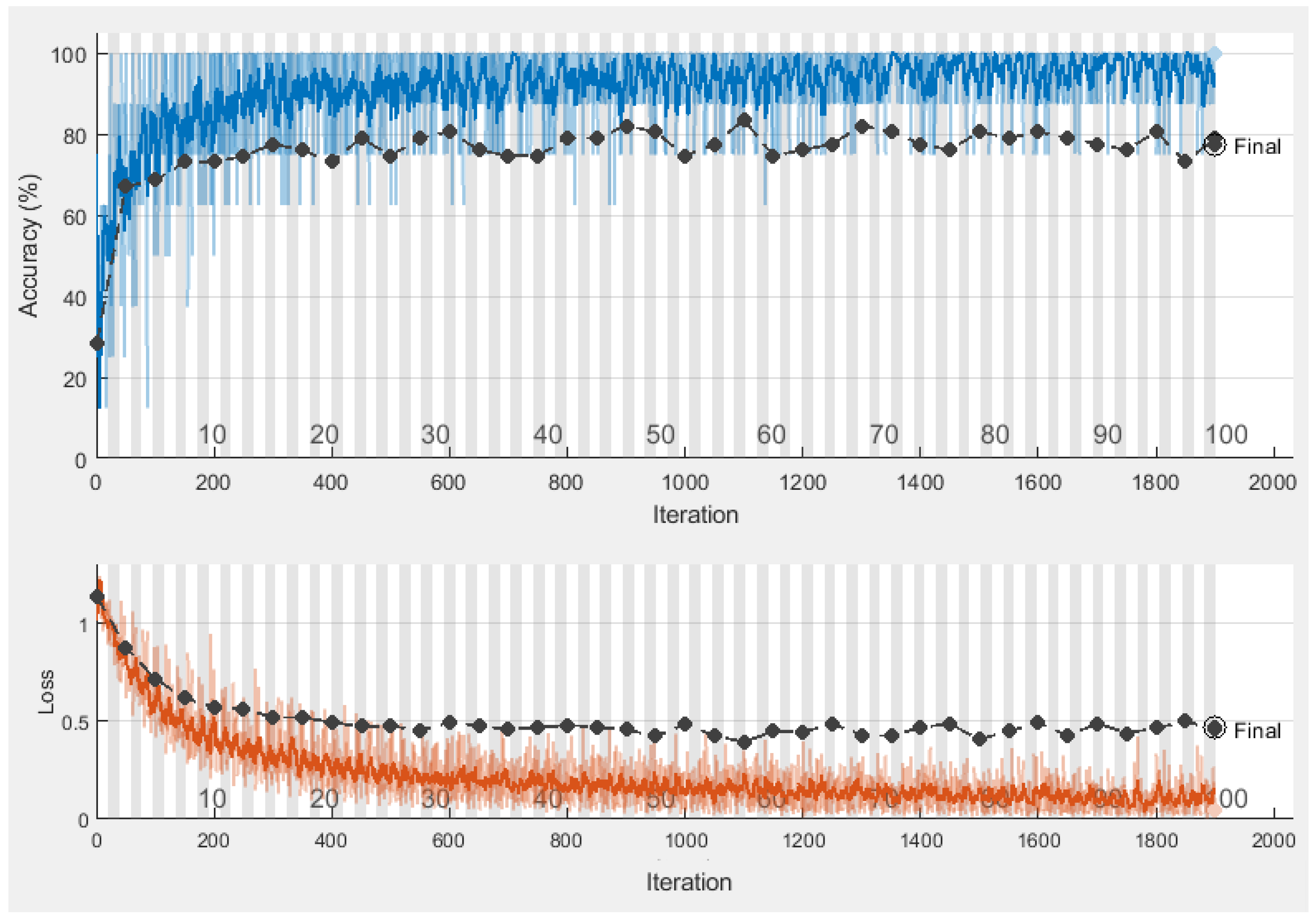
Table 4 indicates a proposed CNN’s optimal parameters with the most accurate found CNN as 77.62% validation accuracy. The training time with different values is validated to improve the accuracy. Therefore, the performance-based selection of CNN is used with the given parameters of CNN. The training and validation graph is shown in Figure 5.

Figure 5 designates the absolute accuracy by finding the 77.62% as validation accuracy where the loss is up to 0.5 with a bit of variation. The data-specific learning of a given data set is more favorable as it covers all aspects of features, such as location, geometry, or other local features. At this stage, the feature vector is taken as transfer learning to get the numeric features from the CNN fully connected layer encodings. The activated features are then later used as a classification feature vector.

3.1. Data Splitting

The activated features are of size n × 3, where all image features are split up with randomization to remove the data’s biases. The used data split ratios are 50–50% (training, testing), 60–40% (training-testing), and 70–30% (training, testing). All data divisions employ seven different classifiers.

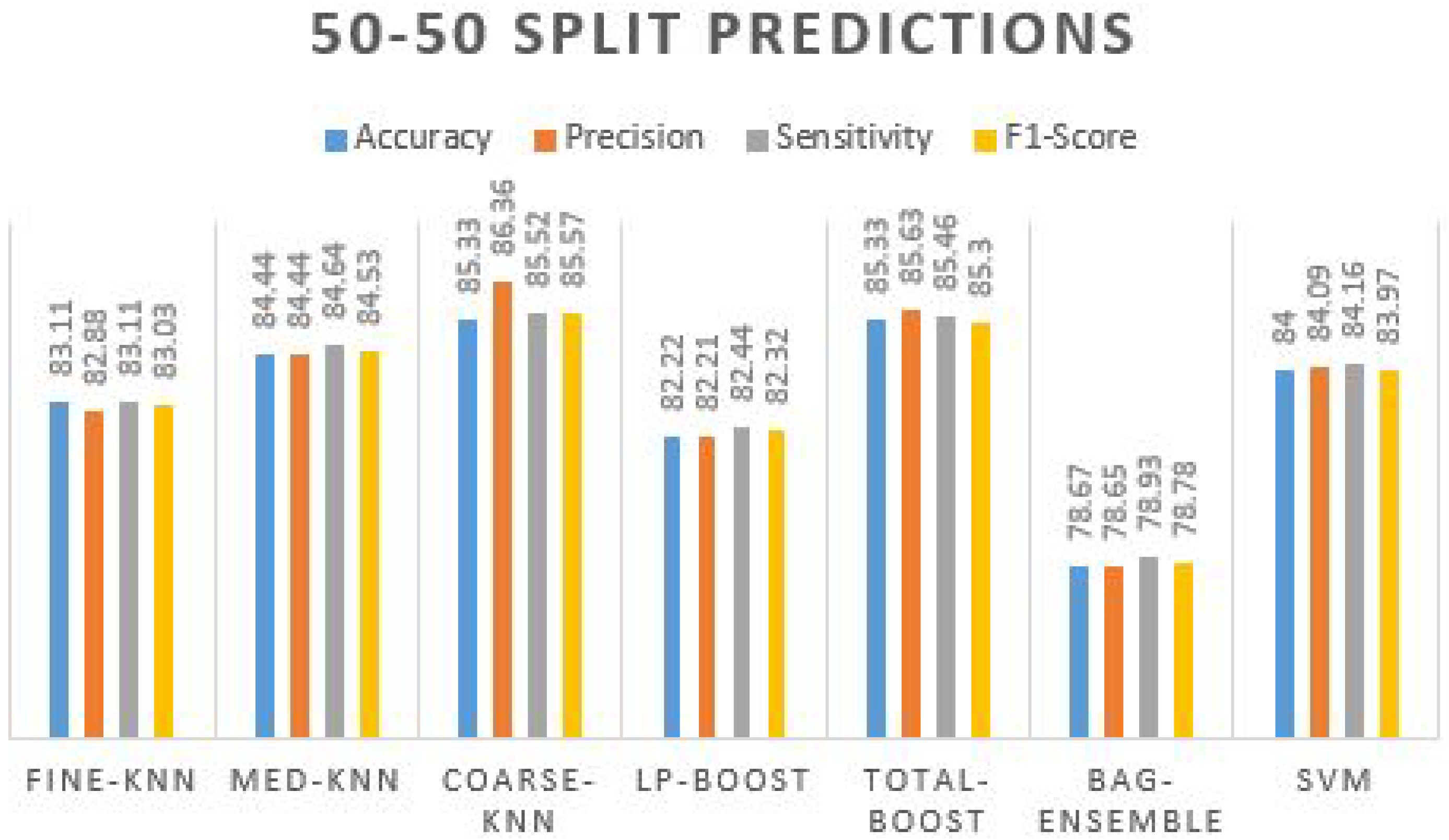
3.2. Experiment 1 (50–50)

In the first experimental phase, we split the features vectors as 50% for training and 50% for testing. The features matrix displays 225 × 3 and 225 × 3 for training and testing vectors. The trained classifiers-based predictions are then evaluated in terms of accuracy, precision, sensitivity, and F1 score. Moreover, a statistical evaluation metric such as Kappa has also been computed to evaluate the results. The prediction results are given in

Table 5. Results obtained using different ML classifiers on 50–50 Split.

Method	Accuracy (%)	Precision (%)	Sensitivity (%)	F1-Score (%)	Kappa
Fine-KNN	83.11	82.88	83.11	83.03	0.62
Medium-KNN	84.44	84.44	84.64	84.53	0.65
Coarse-KNN	85.33	86.36	85.52	85.57	0.67
LP-Boost	82.22	82.21	82.44	82.32	0.60
Total-boost	85.33	85.63	85.46	85.30	0.67
Bag-Ensemble	78.67	78.65	78.93	78.78	0.52
SVM	84.00	84.09	84.16	83.97	0.64

.

Table 5 has bestowed that the maximum prediction accuracy is achieved by two classifiers, including 85.33% by coarse-knn and total-boost. The additional algorithms also performed well, with the accuracy range nearer to the two best-achieved algorithms. Their accuracy remains in the range of 80%+, where the accuracy obtained using the bag-ensemble method is not promising. Prediction plots obtained using different ML classifiers on 50–50 split are given in Figure 6.

We can observe that other performance measures of classification predictions are also higher as the precision value is 86.36% by coarse-knn, which is more reliable than the precision obtained using the total-boost method. Hence, in terms of more true optimistic predictions over the summation of true positives and false positives, = the sensitivity and F1s-core are also improved by the coarse-knn compared to other classifiers. The confusion matrix obtained using Coarse-KNN is presented in

Table 6. Confusion matrix obtained using Coarse-KNN.

Classes	Khundi	Mix	Neli-Ravi
Khundi	66	8	1
Mix	20	57	0
Neli-Ravi	3	1	69

.

The confusion matrix of coarse-knn indicated that the accurately predicted instances do not satisfy the Mix class as 20 instances are wrongly predicted in the khundi target class that belongs to the Mix class. However, the correctly predicted number of instances is 192 in total.

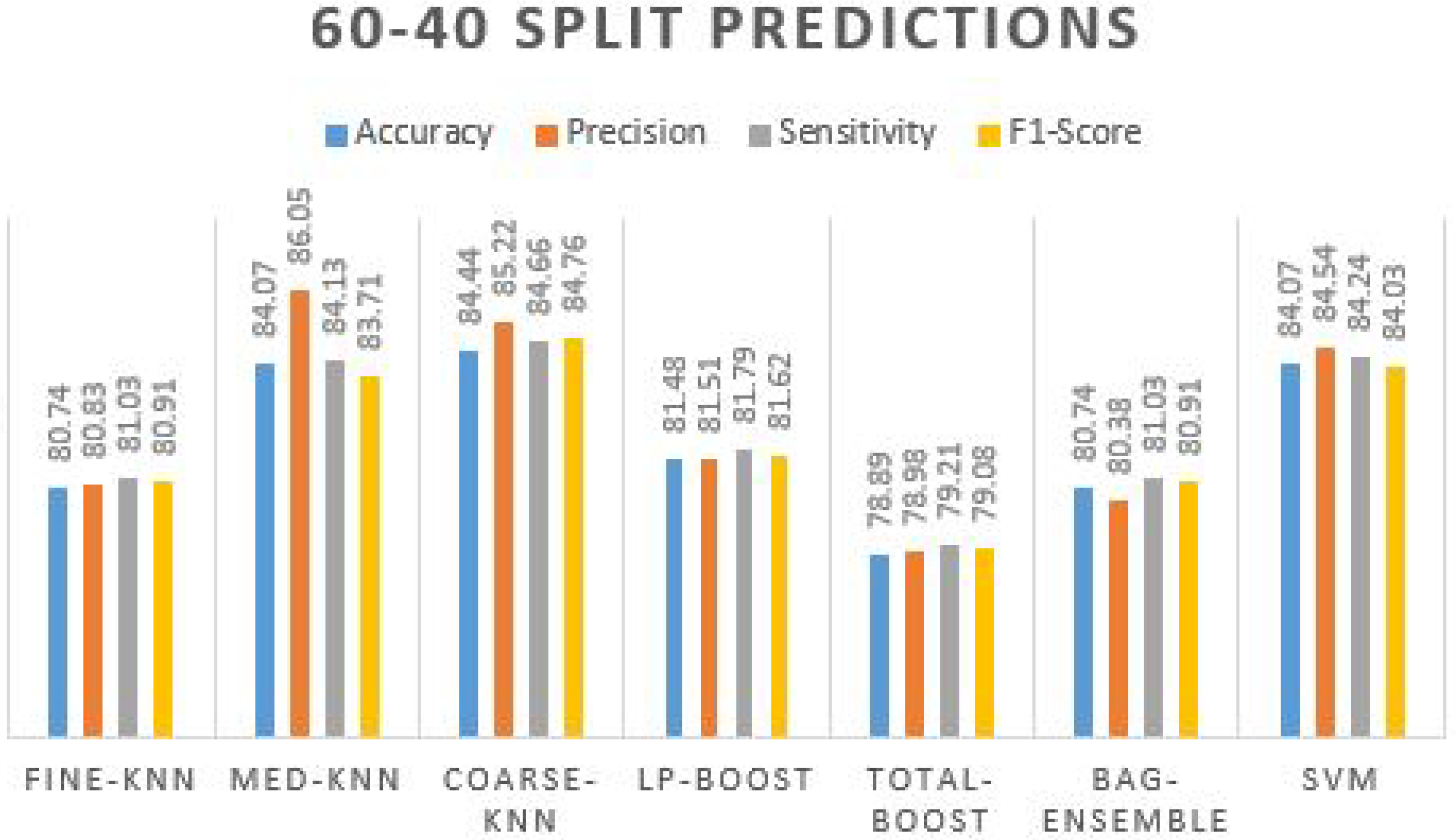
3.3. Experiment 2 (60–40)

Experiment 2 uses features vectors obtained from the last layer of self-activated CNN, splitting into 60–40% with 60% for training and 40% for testing. The overall results were almost identical to the 50–50 split strategy. Results obtained using different ML classifiers on 60–40 Split are presented in

Table 7. Results obtained using different ML classifiers on 60–40 split.

Method	Accuracy (%)	Precision (%)	Sensitivity (%)	F1-Score (%)	Kappa
Fine-KNN	80.74	80.83	81.03	80.91	0.56
Medium-KNN	84.07	86.05	84.13	83.71	0.64
Coarse-KNN	84.44	85.22	84.66	84.76	0.65
LP-Boost	81.48	81.51	81.79	81.62	0.58
Total-boost	78.89	78.98	79.21	79.08	0.52
Bag-Ensemble	80.74	80.83	81.03	80.91	0.56
SVM	84.07	84.54	84.24	84.03	0.64

.

In Table 7, we can observe that the coarse-knn got the highest accuracy (84.44%) with slightly less accuracy precision, sensitivity, F1-score, and kappa values. Moreover, the other classifiers also perform in the range of 80%+. We can see in the 2nd row; the medium-knn achieved 84.07% accuracy. Similarly, SVM achieved the same accuracy value but with a lower precision rate of 84.54%. Fine-knn and bag-ensemble obtained the same accuracy value of 80.74% with all the same other evaluation measures. A prediction plot obtained using different ML classifiers on 60–40 split is displayed in Figure 7.

The first and second phases of experimental chunks obtained almost the same results, which were more promising as different classifiers of different categories providing almost identical accuracy values—the most accurate classifier’s prediction-based confusion matrix is shown in

Table 8. Confusion matrix obtained using SVM.

Classes	Khundi	Mix	Neli-Ravi
Khundi	76	13	1
Mix	23	70	0
Neli-Ravi	3	2	82

. The primarily used conventional 70–30% split ratio is also utilized for more confident results.

The confusion matrix identified that the khundi class predictions are more accurate, whereas the ‘Mix’ class needs more improvement. The 76, 70, and 82 are the accurate predictions, whereas the wrongly predicted numbers are 13,1 and 23,3 and 2. Those wrongly predicted instances are on the upper and lower diagonal of the table.

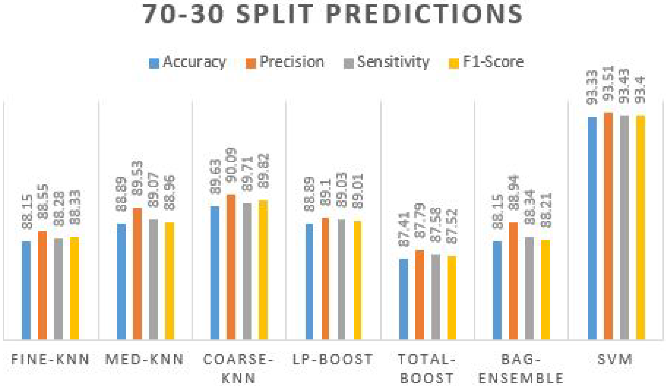
3.4. Experiment 3 (70–30)

In the third experiment phase, we performed experiments using standard 70% random features splitting with 30% data testing. The evaluation measures are the same as in experimental phases one and two. The obtained results show gradual improvements as compared to the previous ones. Results obtained using different ML classifiers on 70–30 split are exhibited in

Table 9. Results obtained using different ML classifiers on 70–30 Split.

Method	Accuracy (%)	Precision (%)	Sensitivity (%)	F1-Score (%)	Kappa
Fine-KNN	88.15	88.55	88.28	88.33	0.73
Medium-KNN	88.89	89.53	89.07	88.96	0.75
Coarse-KNN	89.63	90.09	89.71	89.82	0.76
LP-Boost	88.89	89.10	89.03	89.01	0.75
Total-boost	87.41	87.79	87.58	87.52	0.71
Bag-Ensemble	88.15	88.94	88.34	88.21	0.73
SVM	93.33	93.51	93.43	93.40	0.85

.

In Table 9, the maximum accuracy recorded using SVM is 93.33%, with the most accurate precision value. The given accuracy of this phase is justified and reportable. The other classifiers also display more than 87% accuracy. A prediction plot obtained using different ML classifiers on a 70–30 split is manifested in Figure 8.

It is observed that in all experiments, the performance measure does not vary. The confusion matrix for the best-achieved accuracy algorithm is also shown in

Table 10. Confusion matrix obtained using SVM on 70–30 split.

Classes	Khundi	Mix	Neli-Ravi
Khundi	42	3	0
Mix	6	40	0
Neli-Ravi	0	0	44

.

The confusion matrix of the most accurate SVM method shows that the Mix class still has more wrong predictions. The overall precision rate is improved to 93.51% over the summation of true positives and false positives. There are fewer wrong predictions in the other two classes; the F1-score provides both precision and a sensitivity response, which is also improved to the extent of 93.40%.

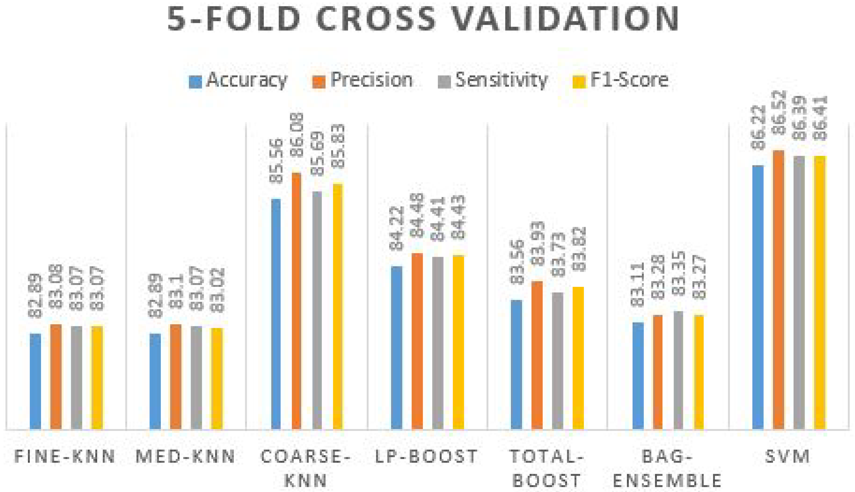
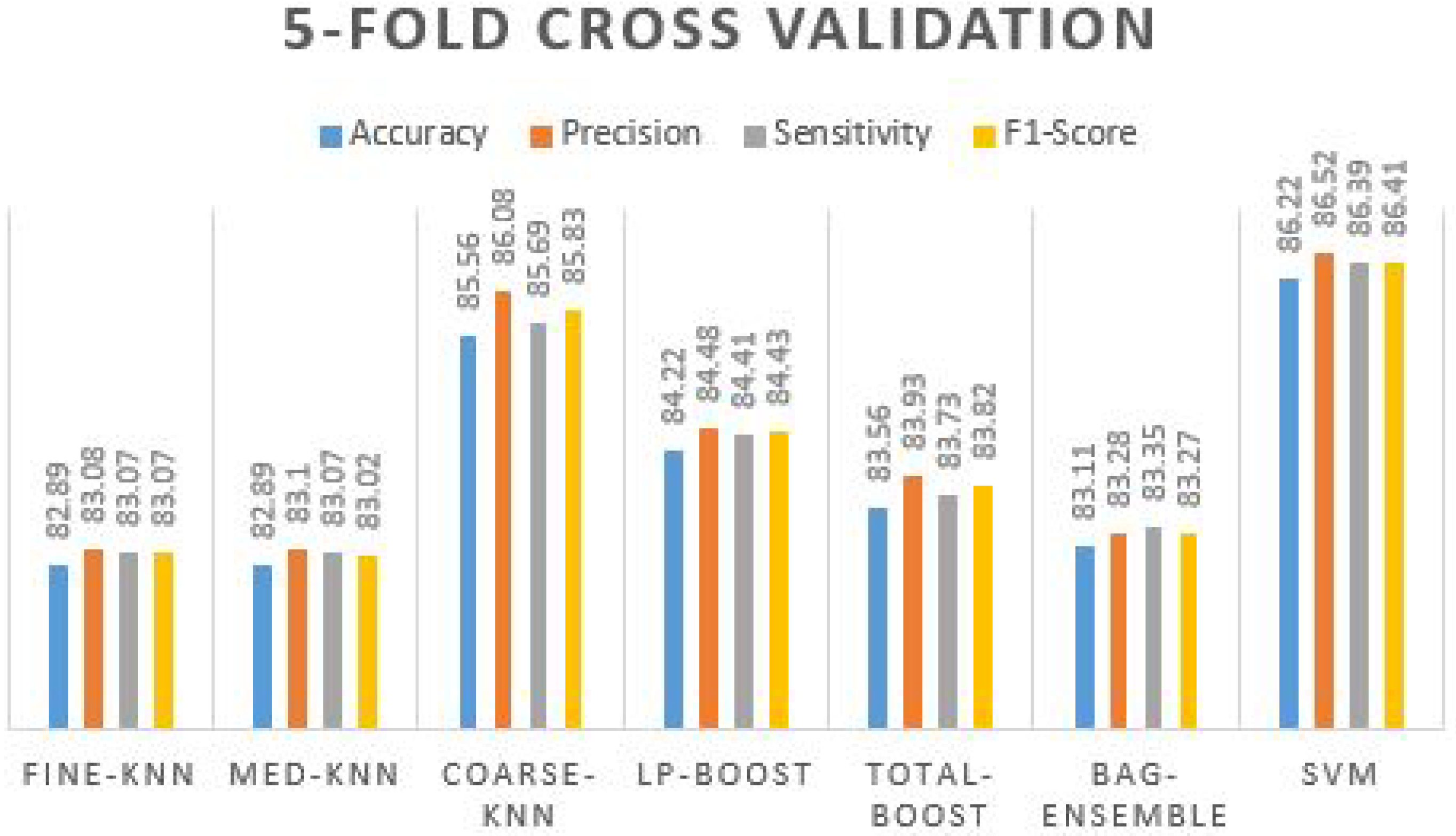
3.5. Experiment 4 (Five-Fold Cross Validation)

After the holdout validation techniques, the results are further evaluated on K-fold cross-validation. The primarily used values for K are 5 and 10 folds on the extracted feature vectors. The results, in this case, were also promising; the results were obtained using different ML classifiers on five-fold cross-validation in

Table 11. Results obtained using different ML classifiers on five-fold cross validation.

Method	Accuracy (%)	Precision (%)	Sensitivity (%)	F1-Score (%)	Kappa
Fine-KNN	82.89	83.08	83.07	83.07	0.61
Medium-KNN	82.89	83.10	83.07	83.02	0.61
Coarse-KNN	85.56	86.08	85.69	85.83	0.67
LP-Boost	84.22	84.48	84.41	84.43	0.65
Total-boost	83.56	83.93	83.73	83.82	0.63
Bag-Ensemble	83.11	83.28	83.35	83.27	0.62
SVM	86.22	86.52	86.39	86.41	0.69

.

Table 11 confirms that coarse-knn and SVM produce the best accuracy and other effects. The accuracy value reaches up to 86.22% with 86.52% precision, 86.39% sensitivity, and 86.41% of the F1-score. By examining the precision value, the true positive value seems to be truer where the F1-score cross-validated it by taking sensitivity and precision over it and again received 86.41%. The prediction plot obtained using different ML classifiers on five-fold cross validation is manifested in Figure 9.

We can see from the graph that all five other classifiers are above 80% to 84% of the accuracy values, where coarse-knn and SVM have accurate results. Furthermore, we evaluated the proposed framework on 10-fold validation to ensure the extracted feature vectors’ integrity.

3.6. Experiment 5 (10-Fold Cross Validation)

All extracted features are given to 10-fold validation, making each split during the training and validation tenfold. All the results have appeared approximately similar to the five-fold cross-validation; no significant degradation seems in any instance of performance. Results obtained using different ML classifiers on 10-fold cross-validation are presented in

Table 12. Results obtained using different ML classifiers on 10-fold cross validation.

Method	Accuracy (%)	Precision (%)	Sensitivity (%)	F1-Score (%)	Kappa
Fine-KNN	83.56	83.79	83.73	83.76	0.63
Medium-KNN	84.00	84.12	84.21	84.15	0.64
Coarse-KNN	85.11	85.76	85.29	85.38	0.67
LP-Boost	83.78	83.96	83.96	83.96	0.64
Total-boost	83.78	84.10	83.99	84.00	0.64
Bag-Ensemble	84.22	84.36	84.42	84.39	0.65
SVM	85.56	85.74	85.75	85.71	0.68

.

In Table 12, again coarse-knn and SVM received the highest accuracy results, with more than 85% accuracy and more than 85% of precision, sensitivity, and F1-score. The prediction plot obtained using different ML classifiers on 10-fold cross validation is displayed in Figure 10.

It is observed that the performance of overall classifiers is improved. This indicates that higher training folds can increase the performance of all the methods used. The SVM confusion matrix is shown in

Table 13. Confusion matrix obtained using SVM on five-fold cross validation split.

Classes	Khundi	Mix	Neli-Ravi
Khundi	124	24	2
Mix	33	121	0
Neli-Ravi	3	0	143

and

Table 14. Confusion matrix obtained using SVM on 10-fold cross validation split.

Classes	Khundi	Mix	Neli-Ravi
Khundi	121	27	2
Mix	35	119	0
Neli-Ravi	1	0	145

.

It seems that the ‘Mix’ class is devising inaccuracy, which suggests it may contain both types of features of Neli-Ravi and Khundi. However, the Neli-Ravi and Khundi were classified more accurately.

The evaluation metrics used for the experiments are given in the Equations (9)–(12).

$$Precision=100\times \left(\frac{T_p}{T_p+F_p}\right)$$

(9)

$$Sensitivity=100\times \left(\frac{T_p}{T_p+F_N}\right)$$

(10)

$$F1-Score=100\times (2\times \left(\frac{Precision\times Sensitivity}{Precision+Sensitivity}\right))$$

(11)

$$Accuracy=100\times \left(\frac{T_p+T_N}{T_p+T_N+F_p+F_N}\right)$$

(12)

In evaluation measures, one statistical coefficient is used to validate the results. The value of kappa shows the kappa agreement on predicted values compared to the actual values. The kappa value remains from 0 to 1, showing confidence in the given rules. It provides no agreement on the 0–0.20 value and shows minimal agreement on 0.21 to 0.39. Additionally, it shows a weak agreement from 0.40 to 0.59. The substantial ranges start from 0.60 to 0.90 or above. This shows confident agreement upon a 0.90 to 1 value. However, the calculation is performed using a confusion matrix by obtaining predicted and actual class numbers [31].

$${cm}_n={Margin}_{col}$$

(13)

$${rm}_n={Margin}_{row}$$

(14)

The margin values of the calculated confusion matrix are used for the calculation of Pr (e), which is actually the major nominator value for Equation (16).

$$\mathrm{Pr}\left(e\right)=(\left({cm}_1\times {rm}_1\right)/n+\left({cm}_2\times {rm}_2\right)/n)/n$$

(15)

$$Cohen-Kappa=\frac{\mathrm{Pr}\left(a\right)-\mathrm{Pr}\left(e\right)}{1-\mathrm{Pr}\left(e\right)}$$

(16)

Equation (15) shows the actual calculation of Pr(e). The ${cm}_1$ shows the confusion matrix margin values of all classes, whereas ${rm}_1$ shows the row margin values of the confusion matrix. However, the cohen-kappa shows confidence in its 0.8 to 0.9 strong agreement. We can see from the table that the SVM has a 0.85 value of kappa coefficient, which is a far more substantial value to rely on data content or features.

4. Conclusions

Pakistan’s dairy production centers face issues in identifying and separating the Neli-Ravi breed from other buffalo breeds. As a result, automatic buffalo breed identification and classification are needed. The proposed study utilized the Pakistani buffalos data set for computer-vision-based recognition and Neli-Ravi classification from other buffalo breeds. The proposed deep CNN architecture deduced the spatial information from the buffalo images and assembled the rich feature vectors. Furthermore, a learning-based approach transfers rich features into activated layers for better classification. Several ML-based classifiers are adopted to classify the instances into relevant target classes. The confidence in the data set and features are validated using different data splits, which do not abruptly vary. All results are normalized and reliable, making the proposed research an accurate recognition method for different buffalo breeds. The proposed framework achieves a maximum accuracy of 93%, and using recent versions, it achieves more than 85% accuracy.

In the future, we intend to employ optimized deep-learning-based architectures using optimization algorithms such as genetic algorithm (G.A), bee-swarm optimization (BSO), and the differential evolution algorithm (D.E) to enhance the accuracy.