Wheat Water Deficit Monitoring Using Synthetic Aperture Radar Backscattering Coefficient and Interferometric Coherence

Abstract

Due to the climate change situation, water deficit stress is becoming one of the main factors that threatens the agricultural sector in semi-arid zones. Thus, it is extremely important to provide efficient tools of water deficit monitoring and early detection. To do so, a set of Synthetic Aperture Radar (SAR) backscattering and interferometric SAR (InSAR) Sentinel-1 data, covering the period from January to June 2016, are considered over a durum wheat field in Tunisia. We first studied the temporal variation of the InSAR coherence data and the SAR backscattering coefficient as a function of the phenological stage of the wheat. Subsequently, the parameters of the SAR and InSAR coherence images were analyzed with regard to the water stress coefficient and the wheat height variations. The main findings of this study highlight the high correlation (r = $0.88$) that exists between the InSAR coherence and the water stress coefficient, on the one hand, and between the backscattering coefficient, the interferometric coherence, and the water deficit coefficient ($R^2$ = $0.95$ and $RMSE$ = $14\%$), on the other hand. When a water deficit occurs, the water stress coefficient increases, the crop growth decreases, and the height variation becomes low, and this leads to the increase of the InSAR coherence value. In summary, the reliability of Sentinel-1 SAR and InSAR coherence data to monitor the biophysical parameters of the durum wheat was validated in the context of water deficits in semi-arid regions.

1. Introduction

Drought and water deficit are considered to be the main environmental factors that threaten agricultural production by limiting plant growth, photosynthesis, and productivity worldwide [1].

In areas with insufficient rainfall, such as arid and semi-arid regions, efficient water management is highly required as water scarcity is a serious problem, and a proper amount of crop irrigation is essential to maintain the desired crop yield quality and soil conditions.

Durum wheat is the most cultivated plant in the Mediterranean basin [2]. In Tunisia, it is the most cultivated cereal crop in terms of production and cultivated area, with approximately $50\%$ of the total sown area [3]. The climate of Tunisia is arid to semi-arid with water deficit problems [3], which threaten the sustainability of agricultural production [4].

In order to maintain a constant production rate, it is necessary to assess the crop water stress in different growing stages. Timely detection and appropriate intervention could help minimize the risk of crop productivity losses.

In this context, different methods have been investigated to monitor crop water stress. These methods are mainly based on soil water measurements, plant responses, and remote sensing systems.

The classical methods that deal with crop water stress detection are based on in situ soil moisture measurements and meteorological variables to assess the water loss from a soil–plant system [5]. The conventional in situ plant-based approaches that include information from stomatal conductance, leaf water potential, relative water content, and stem and fruit diameter have also been widely adopted since they are more effective than the soil moisture-based approaches [6].

Although reliable, the classical monitoring tools were found to be inadequate in the case of cereal crops, which usually extend over large areas.

Therefore, the exploration of faster and more genuine crop monitoring methods, such as the analysis of remote sensing data, is imperative. Indeed, water stress has been largely monitored by various remote sensing data and methods, including the optical data approach of visible and near-infrared bands [7,8,9,10,11,12,13,14] and the thermal infrared band, which is based on the relationships between the surface temperature and plant transpiration [15,16,17,18,19]. The latter approach is limited due to the optical sensor’s sensitivity to clouds and climatic conditions [20,21].

On the other hand, the radar data system represents a reliable tool in overcoming the constraints encountered by optical remote sensing and ensuring the continuity of information on the Earth’s surface regardless of the climatic (clouds, rain, etc.) and temporal (day-night) conditions [21,22,23]. Several studies have monitored vegetation to detect growth anomalies due to diseases and water stress [19,24,25,26,27,28]. These studies attempted to establish the relationships among the bio-physical parameters of vegetation. In the case of durum wheat, several studies have demonstrated the possibility of relating the radar signal to crop parameters, the LAI, and biomass [29,30,31,32,33,34]. Other works focused on the vegetation water content, a key parameter related to evapotranspiration, which is an indicator of the hydrological cycle and the energetic balance of ecosystems.

Although the different agricultural applications of SAR systems based on the analysis of the backscattering signals and InSAR coherence have been investigated throughout various studies [35,36], the potential of using SAR backscattering jointly with InSAR coherence for water deficit crop monitoring has not been investigated.

In this context, the aim of this work is to evaluate the applicability of Sentinel-1 data InSAR coherence and the backscattering coefficient for detecting the water stress levels at the field scale. Accordingly, we first attempt to analyze the temporal variation of the backscattering coefficient and the InSAR coherence related to durum wheat. Furthermore, a relationship between the water stress coefficient, the biophysical parameter, and Sentinel-1 data is established.

2. Materials and Methods

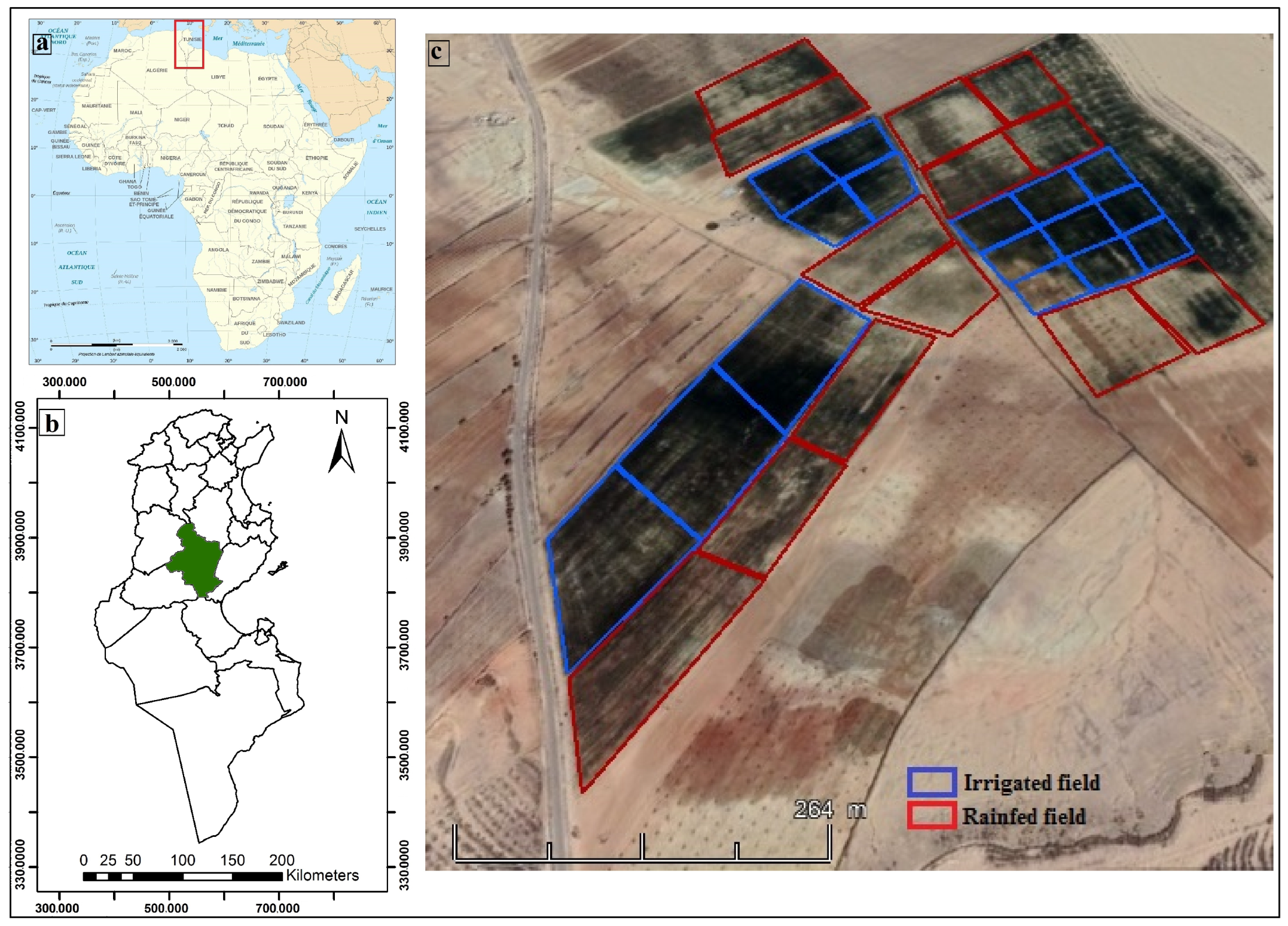
2.1. Study Area

The study site is located in the center of Tunisia in the governorate of Sidi Bouzid (9°21${}^{\prime }$19.68 E and 35°22${}^{\prime }$17.10 N) (Figure 1). This region belongs to the semi-arid bioclimatic stage with an average rainfall of 200–230 mm per year, where the inter- and intra-annual irregularity is very noticeable. The average temperatures are 10 °C for January and 36 °C for July. Cereal farming is conducted in rainfed areas with additional irrigation locally. The monthly rainfall for the 2015–2016 crop year shows that this campaign was characterized by a water deficit of about 260 mm compared to the durum water requirement. Indeed, the average rainfall recorded during this campaign was 190 mm with considerable variability, especially during critical periods of its development such as the tillering stage in February, and the water requirement of durum wheat is 450 to 650 mm.

2.2. Field Data Measurement

Twenty-nine durum wheat fields with the variety “karim” were set up, with 13 in rainfed and 16 in irrigated regimes with an average area of 0.5 ha. The planting was carried out on 15 December 2015, with a density of 120 kg/ha, and the harvest was carried out on 25 June 2016. Five samples were collected for each field, with one sample at the center of the field and one sample at each of the four corners. Figure 2 illustrates the wheat development stages in the investigated fields. All the sampling points were located by the geographical positioning system (GPS). The vegetation on the rainfed and irrigated fields was characterized and the biophysical parameters were measured during every phenological stage of the crop. These parameters include the variables that are related to the vegetation conditions, namely: the phenological stage, the wheat height and Leaf Area Index (LAI), as well as the soil-related variables, i.e., soil moisture, texture, and bulk density. Because these parameters evolve with the phenological cycle, the assessments were carried out for each field and at each phenological stage.

2.2.1. Plant Height Measurements

Throughout the vegetative cycle of wheat, the wheat height measurements were performed for each test plot. The plant heights were measured from the soil surface without changing the plant posture. For each stage, approximately 20 measures covering each plot were randomly collected.

2.2.2. LAI Measurements

The Leaf Area Index (LAI) is the ratio between the surface of the leaves and the surface of the soil on which the vegetation grows.

$$\mathrm{LAI}=\frac{\mathrm{Leaf} \mathrm{area} \left({\mathrm{m}}^2\right)}{\mathrm{Ground} \mathrm{cover} \left({\mathrm{m}}^2\right)}$$

(1)

A series of LAI measurements was carried out in each parcel, which made it possible to obtain different leaf index observations. The measurements were made on the test plots during the different phenological stages using the hemispherical method. Then, the photos were processed using Matlab based on the Hemiview script, which allows batch processing. To do so, an optimal threshold that suites the cover type and the lighting conditions was chosen in order to distinguish between the vegetation pixels and the sky or ground pixels.

2.3. Reference Evapotranspiration ET0

The ET0 was calculated based on the Penman–Monteith formula (1981). The meteorological data, including air temperature, humidity, wind speed, net radiation, and rainfall, were recorded at the weather station of Hajeb Layoun, located 6 km away from the study site. In order to determine the daily reference evapotranspiration ET0 (mm/day), the daily averaged climatic parameters were computed in accordance with the FAO-56 Penman–Monteith parameterization (Equation (2) [37]).

$$\mathrm{ET}0=\frac{0.408\mathsf{\Delta }(\mathrm{Rn}-\mathrm{G})+\gamma \frac{900}{\mathrm{T}+273}{U}_2(\mathrm{es}-\mathrm{ea})}{\mathsf{\Delta }+\gamma (1+0.34U_2)}$$

(2)

where ET0 is the daily reference evapotranspiration (mm/day); Rn is the net radiation at the culture surface (M J/m${}^2$/day); G is the heat flow exchanged with the ground (M J/m${}^2$/day); T is the daily average temperature (°C); $U_2$ is the average wind speed measured at 2 m (m/s); es and ea are, respectively, the saturation vapor pressure and the actual pressure of the air at the same height (kPa); $\mathsf{\Delta }$ is the slope of the saturation vapor pressure curve at the temperature T (kPa /°C); and $\gamma$ is the psychrometric constant (kPa /°C).

2.4. Actual and Potential Evapotranspiration

According to FAO-56, the water needs of a culture are defined by “the amount of water needed to cover the water loss through the evapotranspiration of a healthy crop, grown in a large plot, without soil constraints (fertility and moisture), and realizing its production potential under the conditions considered” [38]. This definition corresponds to the potential evapotranspiration of a culture (PET), which depends on the climatic demand or the reference evapotranspiration (ET0) and the crop coefficient (Kc). To calculate the PET, FAO-56 approach is generally the most used. It is based on Equation (3):

$$\mathrm{PET}=\mathrm{Kc}\times \mathrm{ET}0$$

(3)

The actual evapotranspiration (AET), also called real evapotranspiration, is defined as the sum of the quantities of water vapor evaporated from the soil and the vegetation at a given physiological developmental stage in the presence of water stress.

$$\mathrm{AET}=\mathrm{Ks}\times \mathrm{Kc}\times \mathrm{ET}0$$

(4)

For the present work, we performed the calculations using the FAO formula with the WEAP “water evaluation and planning” software (Version $2015.0$, Stockholm Environment Institute, 2015 [39]).

The crop coefficient (Kc) was calculated directly using the crop coefficient that is proposed by the FAO in its Bulletin No. 56 [38] and then calibrated using the following Equation (5) [40]:

$$K{c}_{stage\left(n\right)}=K{c}_{stage\left(n\right)\left(tab\right)} + [0.04(u_2-2)-0.004(R{H}_{min}-45){\left(\frac{h}{3}\right)}^{0.3}]$$

(5)

where $K{c}_{stage\left(n\right)\left(tab\right)}$ is the standard Kc value proposed by the FAO-56 approach [38], $u_2$ is the daily value of the wind speed at a 2 m height during the development cycle (m/s), $R{H}_{min}$ is the daily value of the minimum relative humidity during the development cycle (%), and h is the height of the crop in (m). In order to verify the calibration of the crop coefficient, the Leaf Area Index (LAI) was measured in situ and the Kc were related. A correlation coefficient of $0.9$ was found.

2.5. Water Stress Index (Ks)

The water stress index (Ks) is related to the soil water reserve, which indicates the water volume that is contained in the soil at a given time. As detailed in (Equation (6)), it makes it possible to take into account the state of the useful soil reserve in the calculation of the evapotranspiration of the crop.

$$\mathrm{Ks}=1-\frac{\mathrm{Actual} \mathrm{Evapotranspiration} \left(\mathrm{AET}\right)}{\mathrm{Potential} \mathrm{Evapotranspiration} \left(\mathrm{PET}\right)}$$

(6)

The water stress index permits determining if the plant is in a water stress condition. When Ks is equal to 0, the plant is in the optimal conditions of development. However, the more the water stress increases, the Ks value will tend to 1.

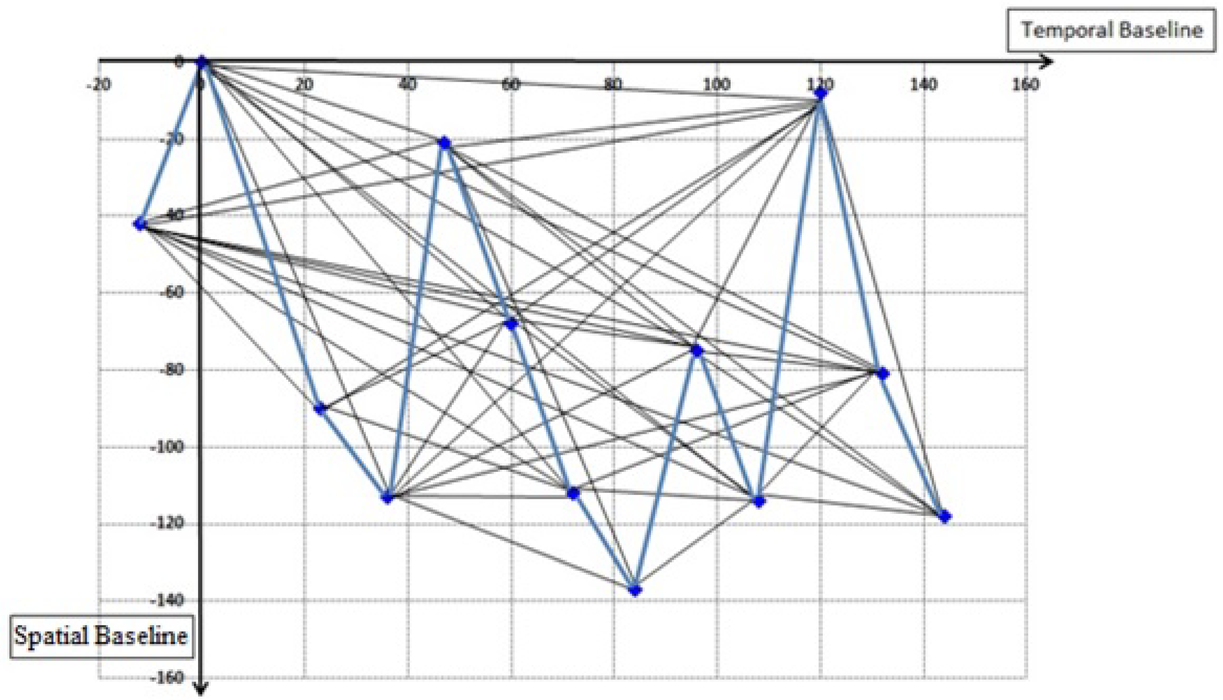
2.6. Remote Sensing Data

Thirteen Sentinel-1 images were acquired during the period from January to June 2016 in interferometric wide swath mode (IW) with a 250 km swath at a spatial resolution of 5 m by 20 m. The mean incidence angle is $37.5^{\circ }$. The data were acquired in ascending pass using vertical-0vertical (VV) and vertical–horizontal (VH) polarization modes. These images were acquired during the same period as the ground measurement. We generated an InSAR coherence image for each of the different pairs and for each polarization (VH and VV). We averaged the coherence over a $3\times 3$-pixel window, to avoid registration and georeferencing errors in order to associate the field measurements with the right sample pixel on the InSAR coherence image. Figure 3 shows a graph of the baseline configurations that were used for the selected InSAR coherence image pairs. The used temporal baseline was 12 days, and the perpendicular baseline was between 23 m and 92 m.

3. Methodology

Our methodology, presented in Figure 4, consists of estimating the empirical relationships between radar signals (sigma VH, sigma VV, coherence VH, and coherence VV) and the coefficient of stress (Ks).

The preprocessing of Sentinel-1 data was performed using SNAP, the available tool of ESA. Then, the backscattering coefficients and the InSAR coherence for the two polarizations VH and VV were calculated at each field. The performance of this relationship was determined by statistical parameters such as the coefficient of determination $R^2$ and the root-mean-squared error (RMSE) using the R package.

4. Experimental Results

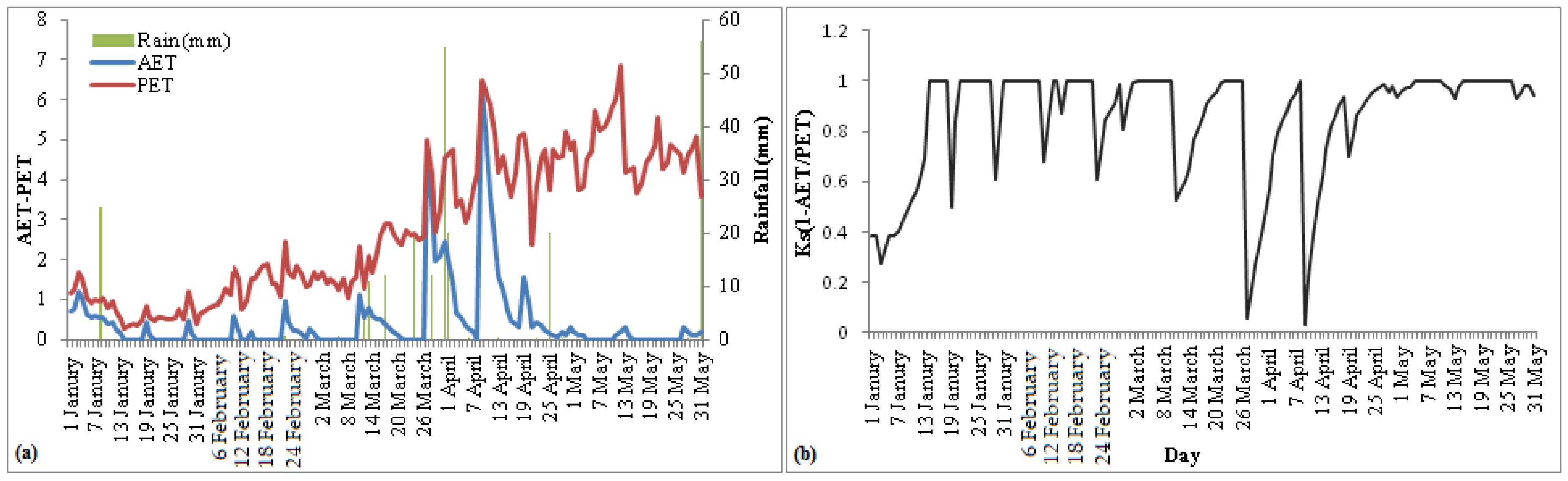
4.1. Temporal Variation of Actual and Potential Evapotranspiration and Water Stress Coefficient

Figure 5a illustrates the results of the actual evapotranspiration, the potential evapotranspiration, and the rainfall analysis. The potential evapotranspiration is proportional to the baseline evapotranspiration and is dependent on the vegetation growth. It increases proportionally with the vegetation cover and reaches its maximum value during the months of March and April, which correspond to the period of the full development of the annual crops. The actual evapotranspiration is very low throughout the crop cycle with the exception of days when there has been precipitation. Moreover, we noticed a significant difference between the actual evapotranspiration and the potential evapotranspiration. This difference is reduced in the rainfall months such as April, which explains the presence of a water deficit during the periods of water shortage [38]. For this reason, $1-\frac{\mathrm{AET}}{\mathrm{PET}}$ represents the water stress index (Ks).

The daily variation of the water stress index is presented in Figure 5b. The results show that, during the majority of the agricultural campaign days, the coefficient of stress is equal to 1, which means a high water stress. The minimum amount of water stress is observed during the months of April and March, when the rainfall was recorded. This water stress, which is observed from the coefficient of water stress, directly influences the development of the crops.

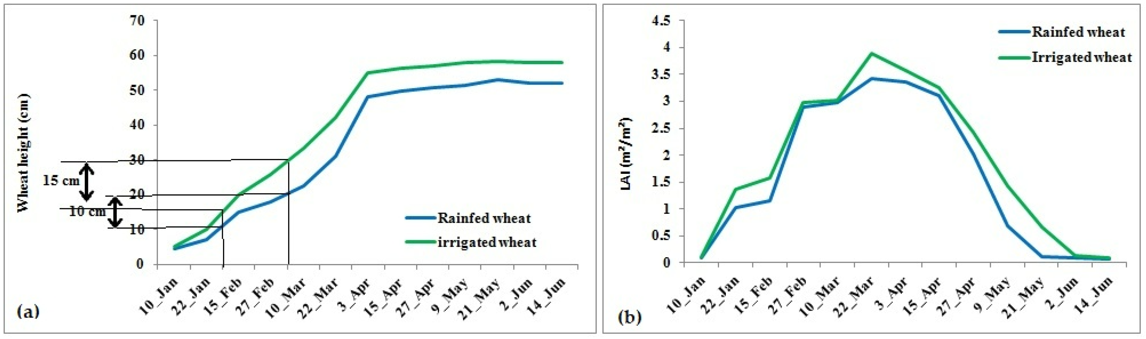
4.2. Temporal Variation of Height and LAI

Figure 6 shows the evolution of the height and LAI during the wheat cycle. A difference between the growth of durum wheat in the rainfed and the irrigated hydrological regimes was noticed in the field. The assessed change in the irrigated wheat height between the two stages was 15 cm, but it was only 10 cm for the rainfed wheat (Figure 6a). This shows the effect of the water deficit on the plants. Furthermore, it was found that the growth of the crop stops before any noticeable lowering, which is perceptible in the relative water content. According to [41], the first effect of water deficit is reducing the growth rate of the stem cells. On the other hand, the LAI values for the irrigated wheat are more pronounced than for the rainfed wheat (Figure 6b). In fact, according to [42], water stress causes a reduction in the leaf area and the height as a sort of adaptation to limit yield losses.

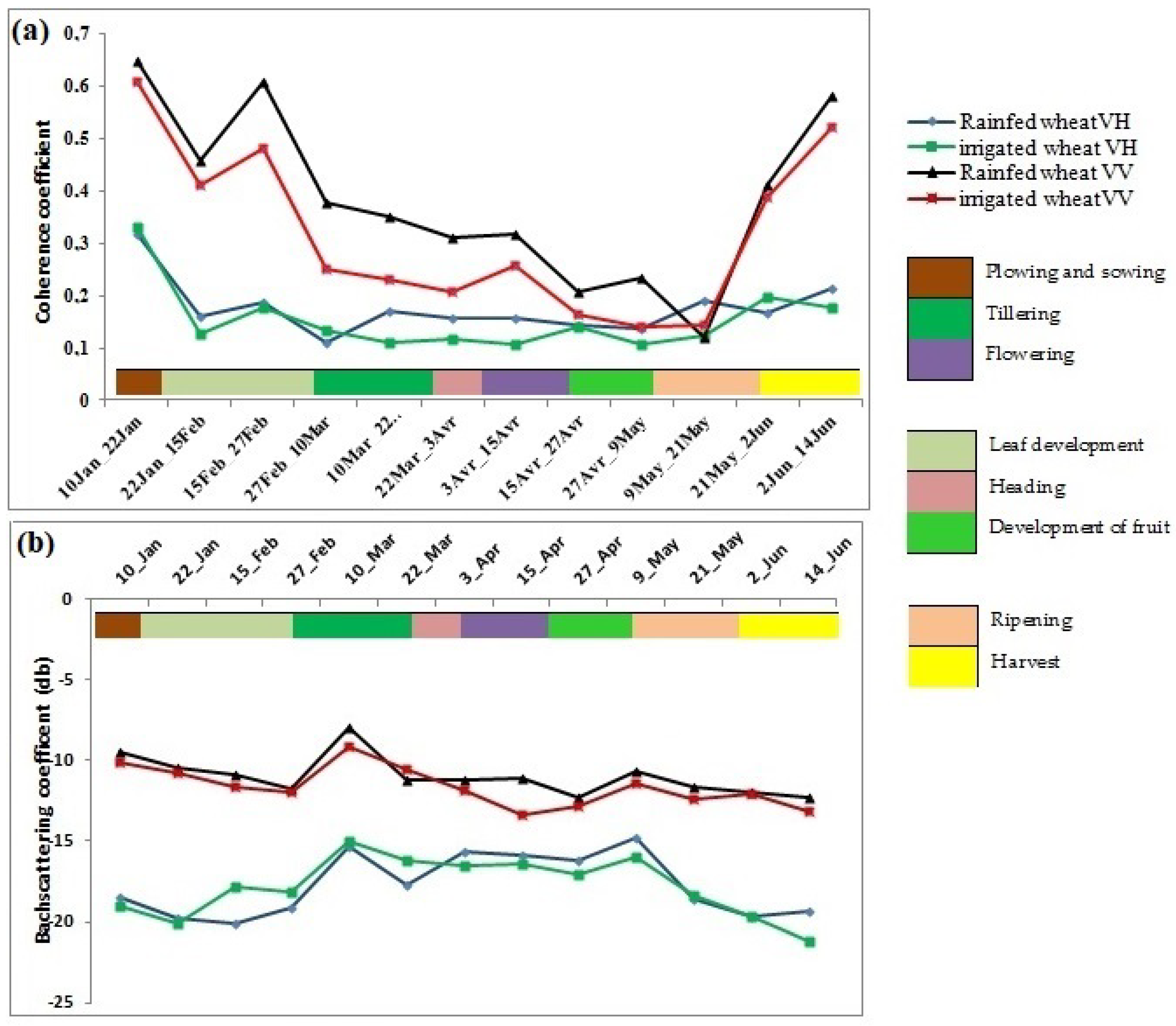
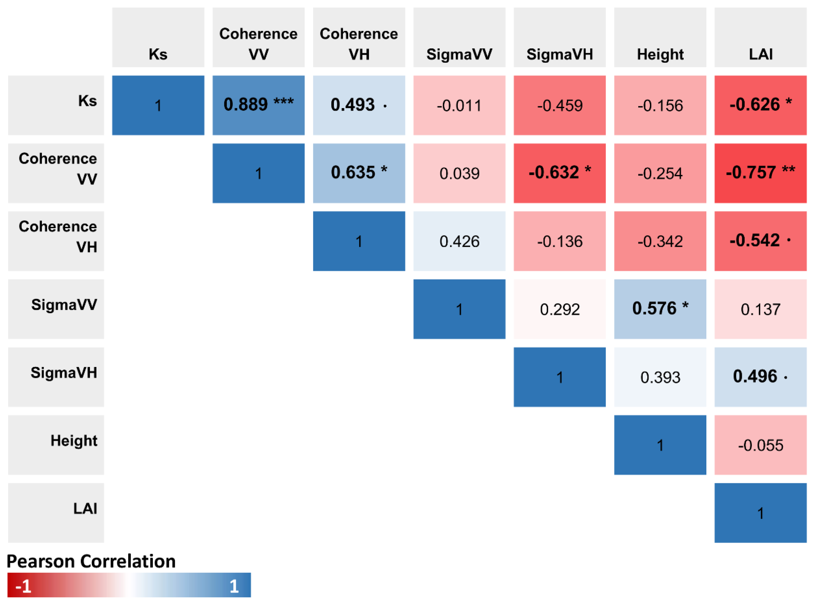
4.3. InSAR Coherence and Backscatter Analysis and Their Relation with Crop Growth

For each stage, the vegetation parameters were recorded in the different field measurements. As shown in Figure 7a, the InSAR coherence value was maximum at the sowing and harvesting stages. The mean coherence values became maximum for the VV polarization and the VH polarization for both irrigated and rainfed wheat. The InSAR coherence values started to decrease with the growth of the plants. At the beginning of the leaf development stage, the ground becomes covered by the plants and the InSAR coherence reaches its lowest value. However, before reaching the harvesting time, an increase was observed in the coherence values for the rainfed and irrigated wheat mainly for VV polarization ($\gamma$ = $0.6$). When comparing the irrigated and rainfed crops, it was noticed that the InSAR coherence values for the irrigated crops were lower, which indicates that their growth variation is more pronounced. Figure 7b shows the changes in the wheat backscatters’ temporal profiles for the growing seasons of all the irrigated and rainfed fields in the study area. There were some minor differences between the averaged temporal profiles of the backscatter of the irrigated and rainfed wheat. During the tillering stage, the backscattering coefficient (${\sigma }_0$) increased from −10 db to −7 db for VV polarization and from −20 db to −15 db for VH polarization. During the mid-stage (i.e., heading, flowering, and development of fruit), the values continued to be constant or showed minor changes.

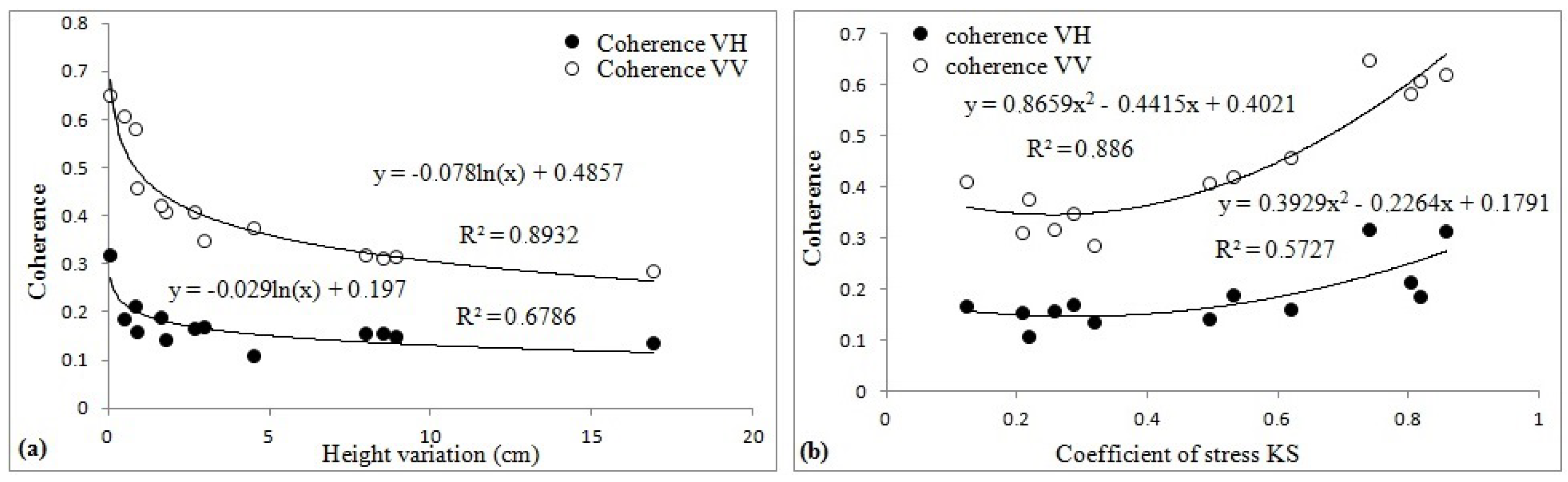
4.4. Detection of Water Deficit Using Interferometric Coherence

The effect of water stress can be observed through the biophysical parameters of the plant, in particular the LAI and the height. During the period of water stress, the increase of the height and the LAI of the plant was low. In this case, the InSAR coherence and the backscattering coefficient can give valuable information about the variation of these biophysical parameters of the plant, which means a better estimation of the water stress coefficient. In fact, the variation of the InSAR coherence between two acquisitions without changes in the soil roughness and moisture is systematically explained by a variation of the crop height and LAI. Basically, the InSAR coherence values vary between 1, which represents a perfect correlation between two SAR acquisitions, and 0, which indicates a total decorrelation between the acquisitions.

Figure 8 illustrates the correlation coefficients between the InSAR coherence, the SAR backscatter, the height variation, the LAI, and the stress coefficient.

The results show a strong correlation between the InSAR coherence and the water stress coefficient Ks when using the VV polarization.

Furthermore, the height of the plant is correlated with the backscattering coefficient at the VV polarization. This is explained by the sensitivity of the vertical polarization VV to the biophysical parameters of the plant.

Figure 9 shows the relation between the InSAR coherence, the variation of the height, and the water stress index (Ks) in Figure 9a,b, respectively. The results show a strong relationship between the coefficient of the stress, the height variation, and the InSAR coherence mainly for VV polarization. The field observations showed that the occurrence of water stress is directly associated with healthy culture development. During the water deficit circumstances, the stress coefficient increases and the variation of the crop growth and the height becomes negligible. This stability in the plant status is represented by an important increase in the InSAR coherence values.

Based on this assumption, we used a multiple regression model to predict the water deficit Ks based on the SAR and InSAR parameters. As detailed in

Table 1. Indicators of the models’ performance that were tested in this study.

	Equation	${\mathit{R}}^2$	RMSE
Model 1	$K_s$ = $-0.31+1.77{\gamma }_{VV}$	$0.74$	$24\%$
Model 2	$K_s$ = $2.068{\gamma }_{VV}+0.25{\sigma }_{0VH}$	$0.95$	$14\%$
Model 3	$Height\ast K_s$ = $-7.4{\sigma }_{0VV}+5.9{\sigma }_{0VH}+132.2{\gamma }_{VV}-111.3{\gamma }_{VH}$	$0.83$	$39\%$
Model 4	$LAI\ast K_s$ = $3.97+0.38{\gamma }_{VV}-5.48{\gamma }_{VH}+0.13{\sigma }_{0VV}+0.06{\sigma }_{0VH}$	$0.4$	$57\%$

, we tested four models:

• The first two models considered Ks as a function of the SAR backscatter and the InSAR coherence data.
• The other two models integrated also the interaction between both Ks with crop height and Ks with LAI values.

The predictive performance of the four models tested in this study were evaluated using the classical accuracy indicators, namely $R^2$ and RMSE. The evaluation of the first model indicates a good $R^2$ and RMSE performance for Ks as a function of the InSAR coherence in the VV polarization. In the second model, the constant used to detect the effect of the other parameters on the Ks was eliminated. In this case, a better performance of the Ks was noticed when considering a function of the InSAR coherence at VV polarization and the SAR backscattering coefficient at VH polarization. In the third model, we found that the introduction of the height did not enhance the prediction of the Ks. However, the introduction of the LAI, in the fourth model, showed no significant results and led to a high RMSE.

5. Discussion

5.1. Variation of the InSAR Coherence and SAR Backscattering Coefficient as a Function of the Wheat Growth Stages

A multi-temporal and multi-polarization analysis, based on the interferometric coherence and the SAR backscattering of Sentinel-1 data, was carried out for durum wheat growth monitoring. The main findings included a significant correlation between the different phenological stages of the wheat and the Sentinel-1 data. In particular, the study pointed out that, before the plowing and after the seeding phases, the InSAR coherence values were high and then sharply decreased once the wheat growing season started. However, during the harvesting stage, the InSAR coherence values significantly increased again. This indicates that the decrease of the InSAR coherence values is mainly related to the dense vegetation during the growth state of the wheat. Thus, the temporal variation of the InSAR coherence can be considered as a key factor in identifying the existence of weak vegetation due to the water deficit stress. The achieved results demonstrated that the InSAR coherence values of the rainfed wheat were higher compared with the irrigated wheat values due to the fact that the vegetation cover of the irrigated crops was denser, which produces more changes between the stages in terms of height, LAI, and biomass. This result is in agreement with [35,43], which analyzed the temporal variation of the InSAR coherence for the wheat crop. Furthermore, according to [43,44], when the geometrical properties of the scatterers (position, orientation, etc.) change, the InSAR coherence decreases. As a result, it is expected to be low in dense vegetation and high in bare soils. Moreover, it was noticed that the InSAR coherence values of the VV acquisitions give a better representation of wheat development than the VH acquisitions. This is explained by the sensitivity of the co-polarization towards the enhanced volume scattering of the vegetation and the lack of the canopy penetration of the VV polarization in the C band [35,45].

Regrading the backscattering coefficient (${\sigma }_0$), during the first two stages: the sowing and leaf development, the backscattering coefficient showed only a few variations. At these stages, the crop height did not exceed 10 cm for all the field samples and the backscattering signal was mainly dominated by the contribution of the bare soil between the crop rows. Several past studies agreed with this result, such as [28,46]. At the tillering stage, the ${\sigma }_0$ increased. This is explained by the fact that the SAR–target interaction, in this stage, depends on both the vegetation and the ground characteristics [47]. Starting from the heading stage, the soil contribution decreased, which caused a rise in the volume scattering mechanisms. According to [12,19], the drop in SAR backscattering values is explained by the existence of the vertical wheat stems and the significant absorption of the incident SAR signal by the leaves, along with a weak direct ground scattering. Furthermore, it was revealed that the temporal change of the SAR backscatter coefficient values does not vary proportionally with the crop size. However, it is mostly dependent on the phenological stage of the crop [31,44,48].

5.2. Estimation of the Water Stress Coefficient Ks

Information from the SAR backscattering and InSAR coherence data has been widely exploited in the context of estimating and monitoring the soil and crop parameters. However, this study brings in new dimensions of information for agricultural studies, especially in detecting the water deficit. According to [41], when the water deficit occurs, the wheat growth stops before the detection of a relative decrease in the water content. In this context, an increase in the InSAR coherence values reflects the stability of the plant cover and, consequently, indicates a very weak growth state of the wheat due to the water deficit. The potential of the InSAR coherence in detecting the height variation was revealed in [44]. It highlighted the sensitivity of the InSAR coherence to the variation of the wheat height and the ability of the Sentinel-1 data to monitor the water deficit. Furthermore, we noticed that the InSAR coherence in the VV polarization achieved better results than the VH polarization, and this can be explained by the sensitivity of this polarization to the height of the crops.

The backscattering coefficient values are sensitive to the soil moisture and the water vegetation content [49,50,51]. Based on this assumption, the backscattering coefficient information of Sentinel-1 was used in [52] to estimate the water stress index. They modeled the actual evapotranspiration and the water stress index as a function of the backscattering coefficient, and they achieved good performance values ($R^2$ = $0.8$). Other studies detected the water stress by modeling the relationship between the SAR-InSAR coherence data, the water vegetation content, and the soil moisture variation [53,54,55,56].

The backscattering information of the VH polarization was found to be better correlated with $Ks$. According to [21,57], VH polarization is more sensitive to the detection of the vegetation water content, whereas VV polarization is more sensitive to the vertical structure, which is represented by the height of the crop. This explains the fact that $Ks$ is determined by the two parameters of the SAR backscatter and InSAR coherence data (${\sigma }_0$ and $\gamma$).

Our results show that the use of Sentinel-1 data can monitor the phenological stage of wheat and estimate Ks. However, the detection of Ks remains indirect, so to improve the results, we can combine SAR data with other remote sensing products, as well as we can track over several agricultural seasons.

6. Conclusions

This work presented a new empirical approach for estimating the stress coefficient (Ks) of durum wheat in a semi-arid area. We used two SAR products: the backscattering coefficient and the InSAR coherence. The results showed that the SAR products were sensitive to the phenological stage of the wheat. A significant correlation among the Ks, height, and SAR products was found. Indeed, when the water deficit occurs, the height variation of the crop decreases and the InSAR coherence value increases. Correspondingly, the hypothesis that the SAR data can detect water deficit was confirmed, and a high correlation was found between the stress coefficient (Ks) and the SAR products (coherence and backscattering coefficient). The present study adopted a straightforward approach that takes advantage of the freely available Sentinel-1 SAR and interferometric SAR data to monitor the water deficit phenomenon. Even though some refinements might still be necessary such as monitoring over several agricultural seasons and the use of other remote sensing products, these results could be applied for future research in water management and irrigation management. Furthermore, they can be considered when developing an operational tool for water management.

References

1. Dellal, I.; McCarl, B.A. The economic impacts of drought on agriculture: The case of Turkey. Options Méditerranéennes 2010, 95, 169–174. [Google Scholar]
2. Elias, E.; Manthey, F.; Stack, R.; Kianian, S. Breeding efforts to develop Fusarium head blight resistant durum wheat in North Dakota. In Proceedings of the 2005 National Fusarium Head Blight Forum, Milwaukee, WI, USA, 11–13 December 2005; pp. 25–26. [Google Scholar]
3. Slama, A.; Ben Salem, M.; Ben Naceur, M.; Zid, E. Les céréales en Tunisie: Production, effet de la sécheresse et mécanismes de résistance. Sécheresse 2005, 16, 225–229. [Google Scholar]
4. Bachta, M.S. L’agriculture, l’agroalimentaire, la pêche et le développement rural en Tunisie. In Les Agricultures Méditerranéennes: Analyses par Pays; CIHEAM: Montpellier, France, 2008; pp. 75–94. [Google Scholar]
5. González-Dugo, M.; Moran, M.; Mateos, L.; Bryant, R. Canopy temperature variability as an indicator of crop water stress severity. Irrig. Sci. 2006, 24, 233–240. [Google Scholar] [CrossRef]
6. Ihuoma, S.O.; Madramootoo, C.A. Recent advances in crop water stress detection. Comput. Electron. Agric. 2017, 141, 267–275. [Google Scholar] [CrossRef]
7. Luquet, D. Suivi de l’état Hydrique des Plantes par Infrarouge Thermique: Analyse Expérimentale et Modélisation 3D de la Variabilité des Températures au Sein d’une Culture en Rang de Cotonniers. Ph.D. Thesis, INA-PG, Paris, France, 2002. [Google Scholar]
8. Ceccato, P.; Flasse, S.; Tarantola, S.; Jacquemoud, S.; Grégoire, J.M. Detecting vegetation leaf water content using reflectance in the optical domain. Remote Sens. Environ. 2001, 77, 22–33. [Google Scholar] [CrossRef]
9. Fensholt, R.; Sandholt, I. Derivation of a shortwave infrared water stress index from MODIS near-and shortwave infrared data in a semiarid environment. Remote Sens. Environ. 2003, 87, 111–121. [Google Scholar] [CrossRef]
10. Schlemmer, M.R.; Francis, D.D.; Shanahan, J.; Schepers, J.S. Remotely measuring chlorophyll content in corn leaves with differing nitrogen levels and relative water content. Agron. J. 2005, 97, 106–112. [Google Scholar] [CrossRef] [Green Version]
11. Duchemin, B.; Hadria, R.; Erraki, S.; Boulet, G.; Maisongrande, P.; Chehbouni, A.; Escadafal, R.; Ezzahar, J.; Hoedjes, J.; Kharrou, M.; et al. Monitoring wheat phenology and irrigation in Central Morocco: On the use of relationships between evapotranspiration, crops coefficients, leaf area index and remotely-sensed vegetation indices. Agric. Water Manag. 2006, 79, 1–27. [Google Scholar] [CrossRef]
12. Hadria, R.; Duchemin, B.; Lahrouni, A.; Khabba, S.; Er-Raki, S.; Dedieu, G.; Chehbouni, A.; Olioso§, A. Monitoring of irrigated wheat in a semi-arid climate using crop modelling and remote sensing data: Impact of satellite revisit time frequency. Int. J. Remote Sens. 2006, 27, 1093–1117. [Google Scholar] [CrossRef] [Green Version]
13. Er-Raki, S.; Chehbouni, A.; Guemouria, N.; Duchemin, B.; Ezzahar, J.; Hadria, R. Combining FAO-56 model and ground-based remote sensing to estimate water consumptions of wheat crops in a semi-arid region. Agric. Water Manag. 2007, 87, 41–54. [Google Scholar] [CrossRef] [Green Version]
14. Er-Raki, S.; Chehbouni, A.; Duchemin, B. Combining satellite remote sensing data with the FAO-56 dual approach for water use mapping in irrigated wheat fields of a semi-arid region. Remote Sens. 2010, 2, 375–387. [Google Scholar] [CrossRef] [Green Version]
15. Kotchi, S.O. Détection du Stress Hydrique par Thermographie Infrarouge: Application à la Culture de la Pomme de Terre. Master’s Thesis, Faculté de Foresterie et Géomatique Université Laval Québec, Québec, QC, Canada, 2004. [Google Scholar]
16. Lili, Z.; Duchesne, J.; Nicolas, H.; Rivoal, R.; de Breger, P. Détection infrarouge thermique des maladies du blé d’hiver 1. Eppo Bull. 1991, 21, 659–672. [Google Scholar] [CrossRef]
17. Courault, D.; Clastre, P.; Guinot, J.; Seguin, B. Analyse des sécheresses de 1988 à 1990 en France à partir de l’analyse combinée de données satellitaires NOAA-AVHRR et d’un modèle agrométéorologique. Agronomie 1994, 14, 41–56. [Google Scholar] [CrossRef] [Green Version]
18. Moran, M.; Clarke, T.; Inoue, Y.; Vidal, A. Estimating crop water deficit using the relation between surface-air temperature and spectral vegetation index. Remote Sens. Environ. 1994, 49, 246–263. [Google Scholar] [CrossRef]
19. Brown, S.C.; Quegan, S.; Morrison, K.; Bennett, J.C.; Cookmartin, G. High-resolution measurements of scattering in wheat canopies-implications for crop parameter retrieval. IEEE Trans. Geosci. Remote Sens. 2003, 41, 1602–1610. [Google Scholar] [CrossRef] [Green Version]
20. Amri, R.; Zribi, M.; Lili-Chabaane, Z.; Wagner, W.; Hasenauer, S. Analysis of C-band scatterometer moisture estimations derived over a semiarid region. IEEE Trans. Geosci. Remote Sens. 2012, 50, 2630–2638. [Google Scholar] [CrossRef]
21. Ulaby, F.T.; Moore, R.; Fung, A. Microwave dielectric properties of natural earth materials. Microw. Remote Sens. 1986, 3, 2017–2027. [Google Scholar]
22. Zribi, M. Développement de Nouvelles Méthodes de Modélisation de la Rugosité Pour la Rétrodiffusion Hyperfréquence de la Surface du sol. Ph.D. Thesis, CGU, Toulouse, France, 1995. [Google Scholar]
23. Adragna, F.; Et Nicolas, J. Traitement des images de Radar à Synthèse d’Ouverture (RSO). In Sous la Direction de Henri Maître; Hermes Science Europe Publication: Paris, France, 2001; Volume 328. [Google Scholar]
24. Holah, N.; Baghdadi, N.; Zribi, M.; Bruand, A.; King, C. Potential of ASAR/ENVISAT for the characterization of soil surface parameters over bare agricultural fields. Remote Sens. Environ. 2005, 96, 78–86. [Google Scholar] [CrossRef] [Green Version]
25. McNairn, H.; Brisco, B. The application of C-band polarimetric SAR for agriculture: A review. Can. J. Remote Sens. 2004, 30, 525–542. [Google Scholar] [CrossRef]
26. Moran, M.S.; Alonso, L.; Moreno, J.F.; Mateo, M.P.C.; De La Cruz, D.F.; Montoro, A. A RADARSAT-2 quad-polarized time series for monitoring crop and soil conditions in Barrax, Spain. IEEE Trans. Geosci. Remote Sens. 2011, 50, 1057–1070. [Google Scholar] [CrossRef]
27. Vereecken, H.; Weihermüller, L.; Jonard, F.; Montzka, C. Characterization of crop canopies and water stress related phenomena using microwave remote sensing methods: A review. Vadose Zone J. 2012, 11, vzj2011-0138ra. [Google Scholar] [CrossRef]
28. Fieuzal, R.; Baup, F.; Marais-Sicre, C. Monitoring wheat and rapeseed by using synchronous optical and radar satellite data—From temporal signatures to crop parameters estimation. Adv. Remote Sens. 2013, 2, 33222. [Google Scholar] [CrossRef] [Green Version]
29. Hajj, M.E.; Baghdadi, N.; Belaud, G.; Zribi, M.; Cheviron, B.; Courault, D.; Hagolle, O.; Charron, F. Irrigated grassland monitoring using a time series of terraSAR-X and COSMO-skyMed X-Band SAR Data. Remote Sens. 2014, 6, 10002–10032. [Google Scholar] [CrossRef] [Green Version]
30. Le Toan, T.; Laur, H.; Mougin, E.; Lopes, A. Multitemporal and dual-polarization observations of agricultural vegetation covers by X-band SAR images. IEEE Trans. Geosci. Remote Sens. 1989, 27, 709–718. [Google Scholar] [CrossRef]
31. Mattia, F.; Le Toan, T.; Picard, G.; Posa, F.I.; D’Alessio, A.; Notarnicola, C.; Gatti, A.M.; Rinaldi, M.; Satalino, G.; Pasquariello, G. Multitemporal C-band radar measurements on wheat fields. IEEE Trans. Geosci. Remote Sens. 2003, 41, 1551–1560. [Google Scholar] [CrossRef]
32. Dente, L.; Satalino, G.; Mattia, F.; Rinaldi, M. Assimilation of leaf area index derived from ASAR and MERIS data into CERES-Wheat model to map wheat yield. Remote Sens. Environ. 2008, 112, 1395–1407. [Google Scholar] [CrossRef]
33. Fontanelli, G.; Paloscia, S.; Zribi, M.; Chahbi, A. Sensitivity analysis of X-band SAR to wheat and barley leaf area index in the Merguellil Basin. Remote Sens. Lett. 2013, 4, 1107–1116. [Google Scholar] [CrossRef] [Green Version]
34. Wiseman, G.; McNairn, H.; Homayouni, S.; Shang, J. RADARSAT-2 polarimetric SAR response to crop biomass for agricultural production monitoring. IEEE J. Sel. Top. Appl. Earth Obs. Remote Sens. 2014, 7, 4461–4471. [Google Scholar] [CrossRef]
35. Nasirzadehdizaji, R.; Cakir, Z.; Sanli, F.B.; Abdikan, S.; Pepe, A.; Calò, F. Sentinel-1 interferometric coherence and backscattering analysis for crop monitoring. Comput. Electron. Agric. 2021, 185, 106118. [Google Scholar] [CrossRef]
36. Khabbazan, S.; Vermunt, P.; Steele-Dunne, S.; Ratering Arntz, L.; Marinetti, C.; van der Valk, D.; Iannini, L.; Molijn, R.; Westerdijk, K.; van der Sande, C. Crop monitoring using Sentinel-1 data: A case study from The Netherlands. Remote Sens. 2019, 11, 1887. [Google Scholar] [CrossRef] [Green Version]
37. Penman, H.L. Natural evaporation from open water, bare soil and grass. Proc. R. Soc. London. Ser. A Math. Phys. Sci. 1948, 193, 120–145. [Google Scholar] [CrossRef] [Green Version]
38. Allen, R.G.; Pereira, L.S.; Raes, D.; Smith, M. Crop Evapotranspiration-Guidelines for Computing Crop Water Requirements-FAO Irrigation and Drainage Paper 56; FAO: Rome, Italy, 1998; Volume 300, p. D05109. [Google Scholar]
39. Sieber, J.; Yates, D.; Huber Lee, A.; Purkey, D. WEAP: A demand priority and preference driven water planning model: Part 1, model characteristics. Water Int. 2005, 30, 487–500. [Google Scholar]
40. Farg, E.; Arafat, S.; Abd El-Wahed, M.; El-Gindy, A. Estimation of evapotranspiration ETc and crop coefficient Kc of wheat, in south Nile Delta of Egypt using integrated FAO-56 approach and remote sensing data. Egypt. J. Remote Sens. Space Sci. 2012, 15, 83–89. [Google Scholar] [CrossRef] [Green Version]
41. Kameli, A.; Lösel, D. Growth and sugar accumulation in durum wheat plants under water stress. New Phytol. 1996, 132, 57–62. [Google Scholar] [CrossRef] [PubMed]
42. Tardieu, F.; Dreyer, E. Regulation of gaseous exchanges in plants under drought stress. In L’eau dans l’espace Rural Production Végétale et Qualité de l’eau; Institut National de la Recherche Agronomique (INRA): Paris, France, 1997; pp. 41–59. ISBN 9782738007087. [Google Scholar]
43. Ouaadi, N.; Jarlan, L.; Ezzahar, J.; Zribi, M.; Khabba, S.; Bouras, E.; Bousbih, S.; Frison, P.L. Monitoring of wheat crops using the backscattering coefficient and the interferometric coherence derived from Sentinel-1 in semi-arid areas. Remote Sens. Environ. 2020, 251, 112050. [Google Scholar] [CrossRef]
44. Engdahl, M.E.; Borgeaud, M.; Rast, M. The use of ERS-1/2 tandem interferometric coherence in the estimation of agricultural crop heights. IEEE Trans. Geosci. Remote Sens. 2001, 39, 1799–1806. [Google Scholar] [CrossRef]
45. Manavalan, R. Review of synthetic aperture radar frequency, polarization, and incidence angle data for mapping the inundated regions. J. Appl. Remote Sens. 2018, 12, 021501. [Google Scholar]
46. Cookmartin, G.; Saich, P.; Quegan, S.; Cordey, R.; Burgess-Allen, P.; Sowter, A. Modeling microwave interactions with crops and comparison with ERS-2 SAR observations. IEEE Trans. Geosci. Remote Sens. 2000, 38, 658–670. [Google Scholar] [CrossRef]
47. Ulaby, F.T.; Kouyate, F.; Brisco, B.; Williams, T.L. Textural infornation in SAR images. IEEE Trans. Geosci. Remote Sens. 1986, 235–245. [Google Scholar] [CrossRef]
48. Fieuzal, R.; Baup, F.; Marais-Sicre, C. Sensitivity of TerraSAR-X, RADARSAT-2 and ALOS satellite radar data to crop variables. In Proceedings of the 2012 IEEE International Geoscience and Remote Sensing Symposium, Munich, Germany, 22–27 July 2012; pp. 3740–3743. [Google Scholar]
49. Zribi, M.; Dechambre, M. A new empirical model to retrieve soil moisture and roughness from C-band radar data. Remote Sens. Environ. 2003, 84, 42–52. [Google Scholar] [CrossRef]
50. Gorrab, A.; Ameline, M.; Albergel, C.; Baup, F. Use of sentinel-1 multi-configuration and multi-temporal series for monitoring parameters of winter wheat. Remote Sens. 2021, 13, 553. [Google Scholar] [CrossRef]
51. Han, D.; Liu, S.; Du, Y.; Xie, X.; Fan, L.; Lei, L.; Li, Z.; Yang, H.; Yang, G. Crop water content of winter wheat revealed with Sentinel-1 and Sentinel-2 imagery. Sensors 2019, 19, 4013. [Google Scholar] [CrossRef] [PubMed] [Green Version]
52. El-Shirbeny, M.; Ali, A.; Mohamed, E.; Abutaleb, K.; Bauomy, E. Monitoring of actual evapotranspiration using remotely sensed data under modern irrigation systems. J. Geograph Environ. Earth Sci. Int. 2017, 12, 1–12. [Google Scholar] [CrossRef]
53. Hanssen, R.F. Radar Interferometry: Data Interpretation and Error Analysis; Springer Science & Business Media: Berlin/Heidelberg, Germany, 2001; Volume 2. [Google Scholar]
54. Gens, R.; Van Genderen, J.L. Review Article SAR interferometry—Issues, techniques, applications. Int. J. Remote Sens. 1996, 17, 1803–1835. [Google Scholar] [CrossRef]
55. Massonnet, D.; Holzer, T.; Vadon, H. Land subsidence caused by the East Mesa geothermal field, California, observed using SAR interferometry. Geophys. Res. Lett. 1997, 24, 901–904. [Google Scholar] [CrossRef]
56. Ouchi, K. Recent trend and advance of synthetic aperture radar with selected topics. Remote Sens. 2013, 5, 716–807. [Google Scholar] [CrossRef] [Green Version]
57. Ulaby, F.; Allen, C.; Eger Iii, G.; Kanemasu, E. Relating the microwave backscattering coefficient to leaf area index. Remote Sens. Environ. 1984, 14, 113–133. [Google Scholar] [CrossRef]
Figure 1. Location of the study area in Sidi Bouzid-Tunisia: (a) Tunisia location; (b) green color is the governorate of Sidi Bouzid; (c) study field, blue outline irrigated field and red outline rainfed field.
Agriculture 12 01032 g001
Figure 2. Crop management and wheat phenological stages in the studies fields.
Agriculture 12 01032 g002
Figure 3. Baseline configuration of the used dataset between 10 January 2016 and 14 June 2016. The lines correspond to interferograms and nodes correspond to SLC images. The bold blue lines represent the baselines between the consecutive images used for coherence analysis. The horizontal axis is the temporal baseline, and the vertical axis shows the perpendicular spatial baseline.
Agriculture 12 01032 g003
Figure 4. Flowchart of the proposed methodology.
Agriculture 12 01032 g004
Figure 5. Daily measurement of actual (AET) and potential evapotranspiration (PET) and rainfall (a). Daily variation of the water stress index (Ks) (b).
Agriculture 12 01032 g005
Figure 6. Wheat height (a) and Leaf Area Index (LAI) (b) variation for irrigated and rainfed wheat; blue line, LAI in rainfed field, and green line, LAI in irrigated field.
Agriculture 12 01032 g006
Figure 7. Temporal variation of: (a) the InSAR coherence coefficient and (b) the backscattering coefficient.
Agriculture 12 01032 g007
Figure 8. Matrix of correlation between sigma VH ( σ 0 V H ), sigma VV ( σ 0 V V ), coherence, LAI, Ks, and height. The cells color is proportional to the strength of the Pearson correlation, ranging from red (negative correlations) to blue (positive correlations), as indicated in the color scale; note: “***”, “**”, “*” and “.” indicate significance at the 0, 0.001, 0.01, 0.05, and 0.1 levels, respectively.
Agriculture 12 01032 g008
Figure 9. Relationship between the InSAR coherence and (a) the height variation and (b) the Ks.
Agriculture 12 01032 g009