A Calibration Method for Contact Parameters of Maize Kernels Based on the Discrete Element Method

Abstract

Clarifying the maize kernel movement during the crushing process is critical for improving the design and optimization of the impact mill. Rather than through experiments, maize kernel movement can be quantitatively analyzed through the discrete element method (DEM), and this could contribute more to the study of the crushing mechanism and equipment optimization. However, having an accurate particle model and contact parameters are prerequisites to ensure the accuracy of the DEM simulation. In this study, we proposed a maize kernel model construction method for the Rocky DEM simulation and a calibration method to calibrate contact parameters. The three-axis size, volume, and shape information of real maize kernels were obtained by 3D scanning, and then the maize kernel model was constructed by the section method. The particle–low-carbon-plate (p–w) and particle–particle (p–p) restitution coefficients were calibrated by using the improved inclined surface drop method. In addition, the angle of repose (AoR) and discharging time were considered together to calibrate the dynamical friction coefficients of p–w and p–p through the funnel method. Additionally, the maize kernel model and calibrated parameter values were used in a DEM simulation of the inclined surface drop test and the funnel test. The maximum relative errors between the simulation values and the measured values of the inclined surface drop test and the funnel test were 4.38% and 6.98%, respectively, which further verified that the proposed maize kernel model construction and contact parameter calibration methods are feasible and accurate. The research method used in this study is a novel idea that can be applied for the construction of the particle model and calibration of the contact parameters of granular materials with complex geometric structures, as well as the maize kernel model, and shows that calibrated contact parameters can provide a reference for the maize kernel crushing simulation to optimize the impact mill.

1. Introduction

1.1. Maize Kernel Movement

Maize kernels are one of the most commonly used cereals in poultry diets worldwide [1]. Crushing is an important process in the journey from maize kernel to feed product. The maize kernel movement plays an important role in the crushing process [2]. Understanding the maize kernel flow behavior during the crushing process is necessary for the design and optimization of the impact mill [3]. Due to the complex working environment and limited available sensors in the crushing processes, it is difficult to quantify the particle movement using traditional experimental methods [4]. Simultaneously, the experimental method for particle motion analysis necessitates the use of expensive experimental equipment, such as a high-speed camera, a laser, and divergent light sheet optics [5], which increases the experimental expense.

1.2. Discrete Element Method

The discrete element method (DEM) has become a common method used in the study of bulk material crushing systems. It can be employed instead of an experiment to quantitatively analyze the movement and breakage of particles [6,7]. The Ab-T10 breakage model in Rocky DEM [8] can better predict the size distribution and shape of progeny particles in crushing simulations, which is helpful for in-depth research on the crushing mechanism and optimization of the mechanical structure [8]. However, to assure the accuracy of the DEM simulation, an accurate particle model and input parameters, including intrinsic and contact parameters, are required. Unfortunately, there are no standard methods for the construction of the particle model and the calibration of contact parameters [9].

In recent years, the construction methods of the particle model have been studied. The approximate representation of real granular material as regular bodies is one of the most common methods [10,11,12]. This is suitable for granular materials with simple structures, such as potatoes and rapeseed grains. Another method is to obtain the contours of the real granular material by 3D scanning, CT, and other technologies, and then fill the contours with spherical particles to complete the particle establishment [6,13,14]. These particles still maintain the structural characteristics of the curved surface, such as in maize kernels and barley grains [15]. However, the breakage models of Rocky DEM only work with convex polyhedral particles for the crushing process simulation, and no spherical, rounded, or concave shape particles are able to be used [16]. Therefore, the above methods are not suitable for particle construction in Rocky DEM, especially for agricultural granular materials with complex structures, such as maize kernels.

One critical step when developing a DEM model is determining the model input parameters, including the intrinsic parameters of granular materials (such as bulk density, Young’s modulus, and Poisson’s ratio) and the contact parameters (mainly the restitution coefficients and friction coefficients of p–w and p–p). The intrinsic parameters can be measured directly or values reported in the literature can be used [6]. However, it is necessary to calibrate the contact parameters in the simulation because of differences in geometry between particles and real granular materials [9]. The method of combining an experiment with a simulation is commonly used to calibrate the contact parameters [9].

The restitution coefficient affects the movement of particles after they collide with the contact surface in the simulation [17,18]. Restitution coefficient calibration methods have been investigated for agricultural granular materials, such as Panax notoginseng seeds, rapeseed, and wheat. One of the common restitution coefficient calibration methods is the trajectory method. High-speed cameras are widely used with the trajectory method to record the trajectories of grains during collisions and calibrate the restitution coefficients of p–w and p–p by changing the parameter values many times until the simulated particle trajectory is consistent with the measured grain trajectory [17,19,20,21]. The high-speed camera is an indispensable part of this method, which increases the cost of the experiment. Additionally, the acquisition and analysis process of the grains’ trajectory is complex, which reduces the calibration efficiency. Therefore, in order to improve the efficiency of the restitution coefficient calibration, the use of a self-made experiment device has become a more effective approach [6,22]. For example, the inclined surface drop method was employed to calibrate the restitution coefficients of potato–contact surface [22], maize kernel–contact surface, and wheat–contact surface [6]. The inclined surface drop method avoids the use of a high-speed camera, which reduces the cost, simplifies the process, and effectively improves the calibration efficiency. Nevertheless, at present, the inclined surface drop method is basically only used to calibrate the restitution coefficient between particles and the contact surface, while the calibration of the p–p restitution coefficient is rarely studied. Friction coefficients (static friction and dynamic friction coefficients of p–w and p–p) are the key parameters affecting particle flow characteristics [21]. At present, the funnel method is commonly used to calibrate friction coefficients, but only a single index like the angle of repose (AoR) or discharging time is used to obtain and calibrate the friction coefficient [6,14,17,20,23,24,25]. In fact, calibrating the friction coefficients with a single index only will reduce the accuracy of parameter calibration [26].

In conclusion, to improve the accuracy of maize kernel crushing process simulation, exploring a maize kernel model construction method suitable for the Ab-T10 breakage model and optimizing the current contact parameter calibration method to improve the accuracy of maize kernel model parameter calibration is critical.

1.3. Aim of the Paper

In order to improve the accuracy of the maize kernel crushing simulation, in this study, we propose a method for maize kernel model construction based on the section method and a method for the calibration of contact parameters involving experiments and simulations using Rocky DEM. The inclined surface drop method device was optimized, and the restitution coefficient for both p–w and p–p were calibrated at the same time. In addition, both the AoR and the discharging time were used as indexes to calibrate the dynamic friction coefficients of the maize kernel by the funnel method [17]. By comparing the simulation and experimental results, the feasibility and accuracy of the maize kernel model and contact parameter values were verified.

2. Materials and Methods

2.1. Experiment Material

Maize kernels are an important raw feed material. According to different feed formulas, the wet basis moisture content of maize kernels in the crushing process ranges from 10% to 17%. Generally, it is best to crush maize kernels with a moisture content of 13% [27]. The maize kernel variety “Xianyu-335,” widely planted in the north and northeast of China, was chosen as the experiment material. Three samples of maize kernels were prepared by following the standard method [28]. The wet basis moisture content of three samples maize kernels was 10.9% ± 0.8 (sample 1), 13.9% ± 0.7 (sample 2), and 17.2% ± 1.2 (sample 3), respectively. The bulk density of the maize kernels in the three samples was 782.57 ± 3.78 g/L, 769.06 ± 1.48 g/L, and 739.00 ± 6.69 g/L, respectively. The wet basis moisture content and bulk density were analyzed by following the standard experiment/formulae [29,30] and are presented as the mean ± standard deviation.

2.2. Physical Experiment

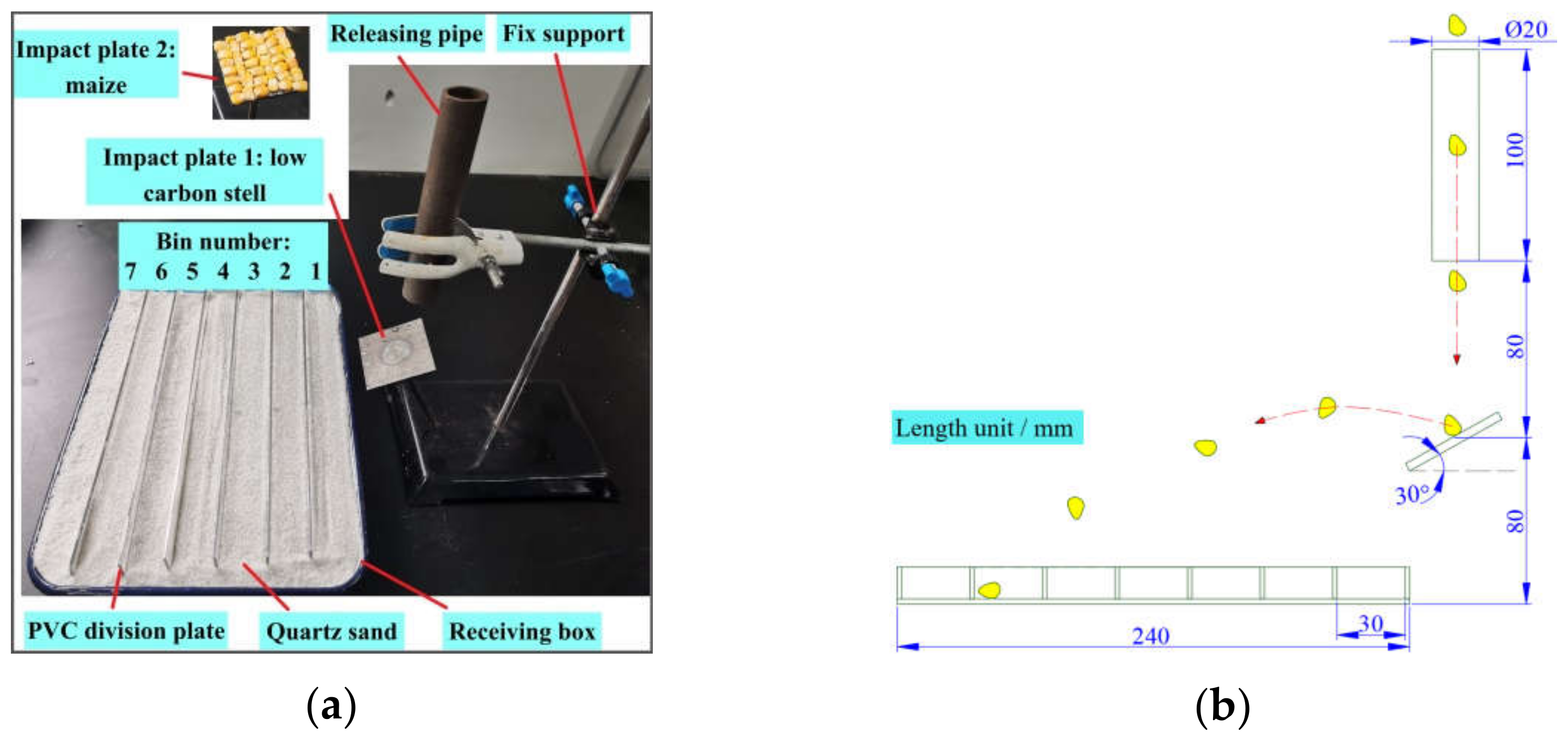
2.2.1. Inclined Surface Drop Method

In order to improve the calibration efficiency and accuracy of the restitution coefficients of p–w and p–p, this study optimized and improved the experiment device of the inclined surface drop method [6]. As shown in Figure 1a, the improved experiment device consists of a particle releasing pipe, a PVC division plate, a particle collection box, and two impact plates, one of which is a low-carbon steel plate (impact plate 1), and the other is a low-carbon steel plate covered with maize kernels (impact plate 2). The geometric dimensions of the experiment device were determined by pre-experiment measures and are shown in Figure 1b. In particular, the spacing of the PVC division plates was set to 30 mm, as suggested by [6].

The particle releasing pipe, the impact plate 2, and quartz sand were added to the improved experiment device. The particle releasing pipe can guarantee that the contact positions of each particle are close to the impact plate, avoiding the influence of the contact position on the particle landing positions and preventing particles from falling out of the particle collection box after contacting the edge of the impact plate. When the particles fall down from the releasing pipe, the result of the collision on impact plate 1 can be used to calibrate the restitution coefficient of p–w. Accordingly, the result of the collision on impact plate 2 can be used to calibrate the restitution coefficient of p–p. As shown in Figure 1a, impact plate 2 is covered with maize kernels. Impact plate 2 was prepared as follows: firstly, a number of maize kernels of uniform particle size and thickness were selected, and then their tip caps were cut off. Secondly, the treated maize kernels were uniformly pasted to the surface of a steel plate with double-sided adhesive. Finally, the steel plate surface with maize kernels was placed downwards on a flat table, and a 5 kg weight was pressed onto the surface of the steel plate and checked every 20 min until the maize kernels were completely fixed and the surface with maize kernels was flat. Subsequently, impact plate 2 was completed. The bottom plate of the particle collection box was uniformly paved with quartz sand to prevent the particles rebounding during the experiment and affecting the accuracy of the experimental results.

For each sample of maize kernels, 300 maize kernels [6] in random orientations were put into the release position and released one-by-one, and then the particles collided with the impact plate. After bouncing off of the impact plate, the maize kernels were collected by the collection box and fell into separate bins, depending on their moving distance after impact. The experiment process is shown in Figure 1b. The number of maize kernels in each bin was recorded. The average bin number (i) was defined as shown in Equation (1). Each experiment was repeated three times to obtain the average bin number in the inclined surface drop experiment. The statistical results are shown in

Table 1. Average bin number of maize kernels.

Contact Type	No. Sample	Average Bin Number of Maize Kernels
p-w	Sample 1	3.91 ± 0.038
	Sample 2	3.80 ± 0.026
	Sample 3	3.55 ± 0.028
p-p	Sample 1	2.86 ± 0.033
	Sample 2	2.75 ± 0.035
	Sample 3	2.55 ± 0.027

.

$$\overline{i}=\frac{1}{N_{total}}{\displaystyle \sum }_{i=1}^n\left(i\times N_i\right)$$

(1)

Here, $\overline{i}$ is the average bin number, i is the bin number, n is the total number of bins, N_i denotes the number of kernels that fall into each bin i, and N_total represents the total number of kernels used in the experiment.

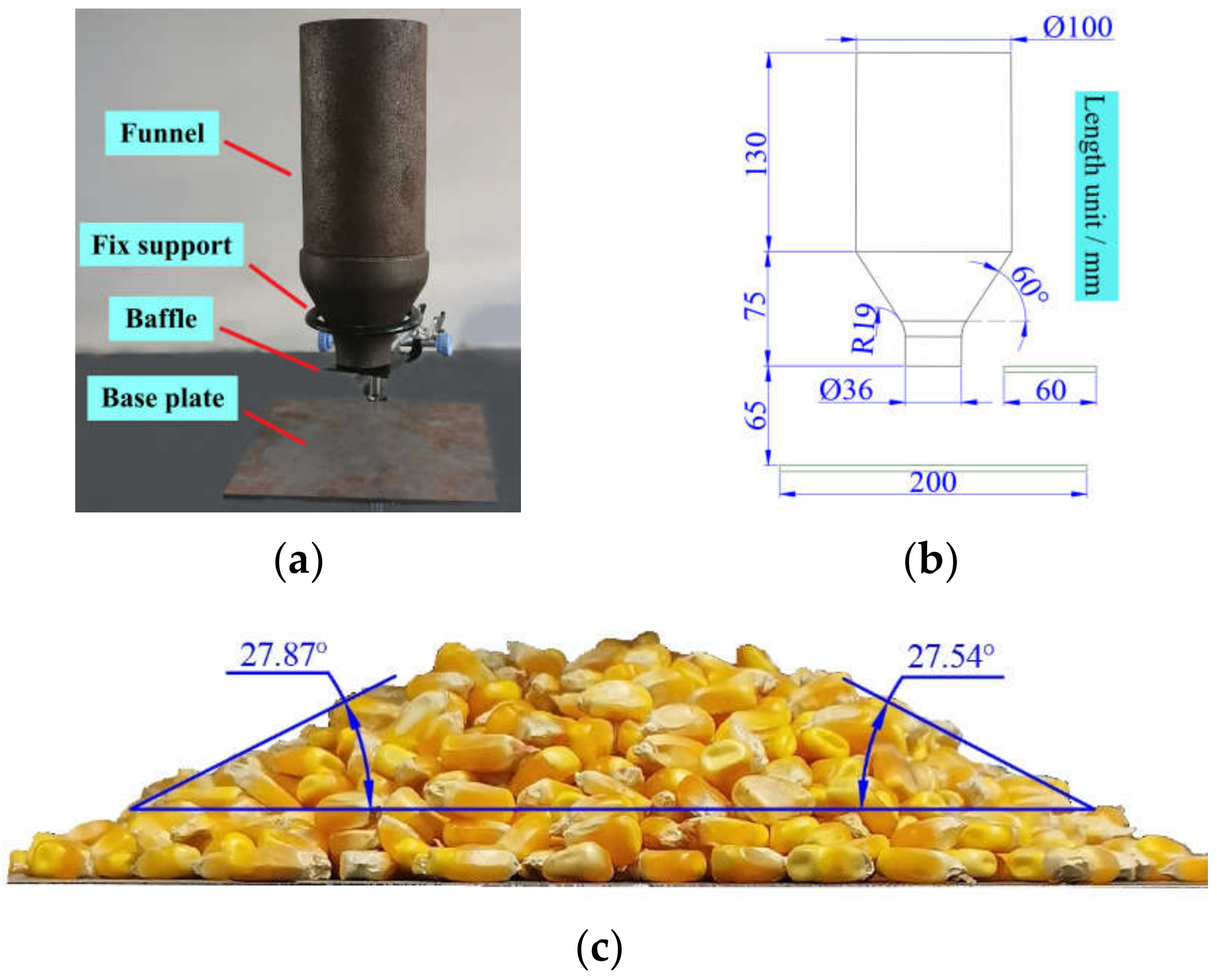
2.2.2. Funnel Method

The funnel method device consists of a funnel, a baffle, a base plate, and a fixed support, as shown in Figure 2a. The geometric dimensions of the experimental device were determined by the pre-experiment measures and are shown in Figure 2b.

The pre-experiment results show that when the mass of maize kernels was 0.45 kg, a stable AoR of maize kernels could be formed, and the AoR would not change as the mass increased. Therefore, 0.45 kg of maize kernels were released into the funnel evenly in the funnel experiment. After standing for 5–10 s, maize kernels in the funnel were basically stationary, and the baffle was quickly pulled out, and the maize kernels to fall evenly on the base plate. Subsequently, the maize kernels gradually formed an AoR, as shown in Figure 2c. In addition, the video of the falling process of the maize kernels was analyzed in a frame-by-frame manner by PotPlayer, and then the discharging time was determined with an accuracy of 0.001 s.

Each group of experiments was repeated 3 times to obtain the mean AoR value and the discharging time, and the results are listed in

Table 2. AoR and discharging time of the maize kernels.

No. Sample	AoR/(°)	Discharging Time/(ms)
Sample 1	27.10 ± 0.93	2320 ± 35.51
Sample 2	28.52 ± 1.26	2382 ± 29.33
Sample 3	29.60 ± 1.07	2583 ± 42.84

.

2.3. Simulation Set-Up

Fundamentally, the DEM solves Newton’s equations of motion to resolve particle motion and uses a contact law to describe the inter particle contact forces. Forces are typically integrated explicitly in time to predict the time history response of the material using an appropriate numerical integration method. The hysteretic linear spring model for normal force calculation and the linear spring Coulomb limit model for tangential force calculation were used to simulate the inclined surface drop test and the funnel test in Rocky DEM [16].

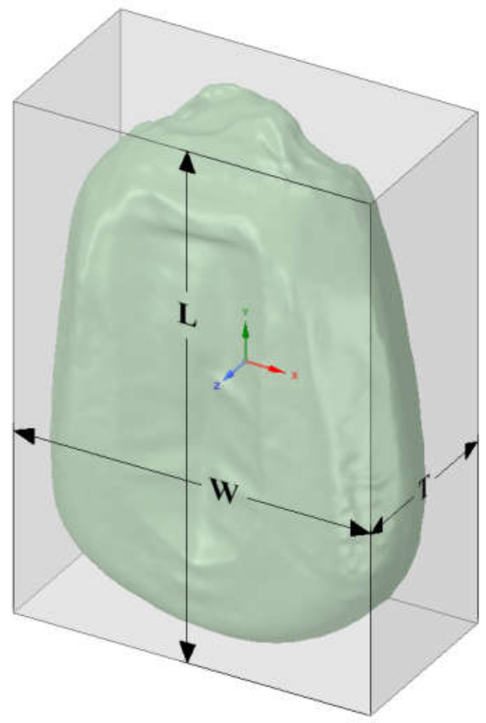
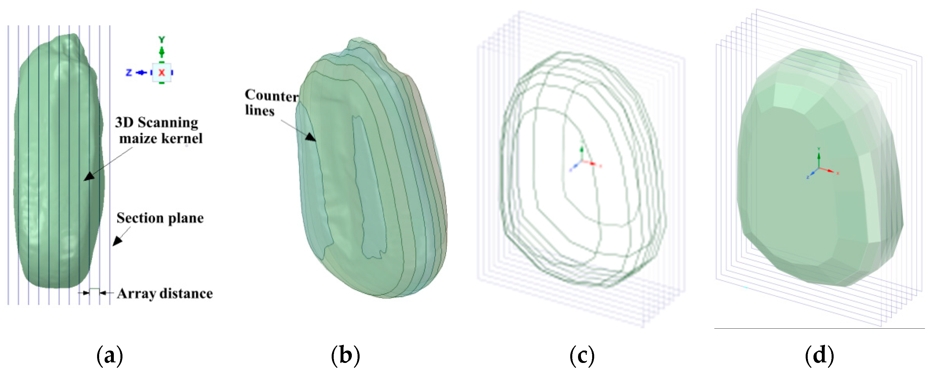
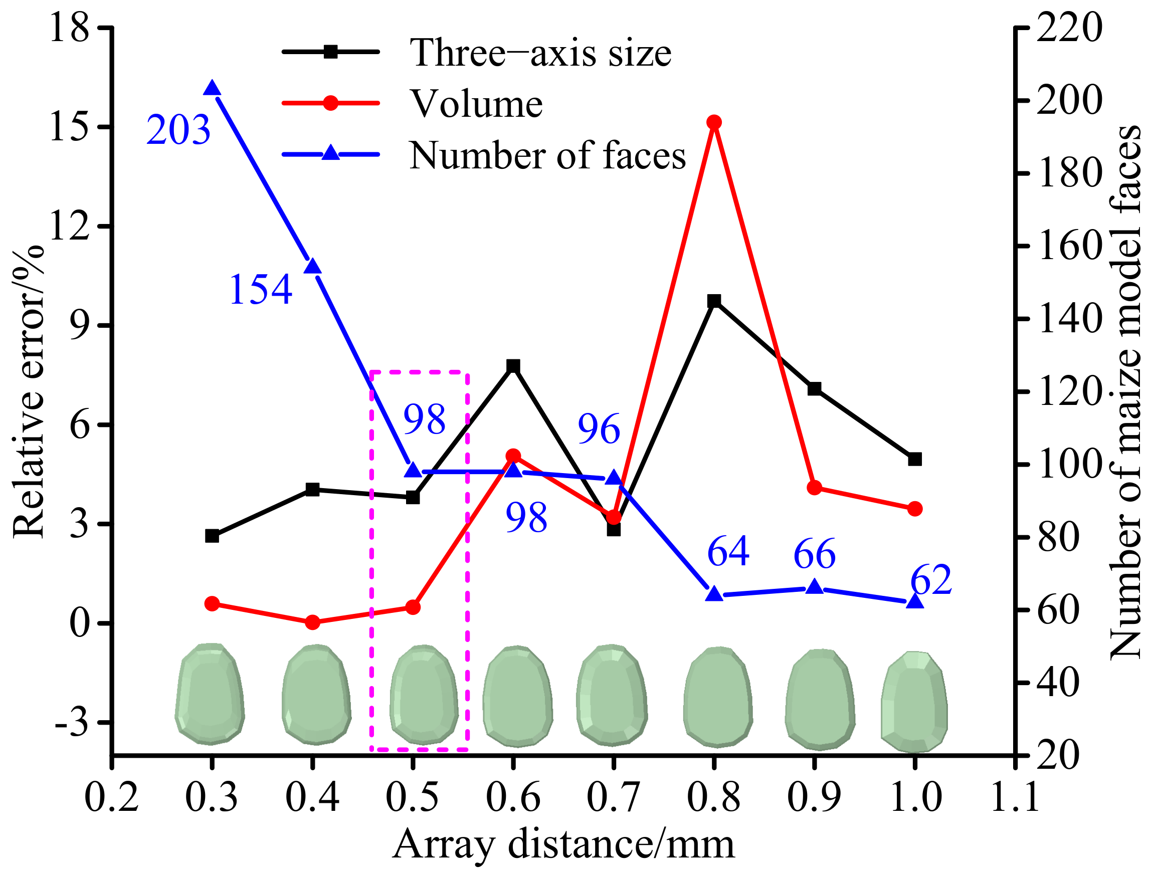
2.3.1. Construction of the Maize Kernel Model

Maize kernels were divided into wedge, ellipsoid, and irregular shapes, among which wedge-shaped maize kernels accounted for the highest proportion of kernels, about 94.72% [31]. The effect of the moisture content on the geometric structure of maize kernels is negligible [32]. Therefore, this study took the wedge-shaped maize kernel from sample 2 as the object to establish the particle model for the DEM simulation. For granular materials with complex geometry, the geometry can be characterized by the sizes of three axes, length (L), width (W), and thickness (T) [33], as shown in Figure 3. In the crushing simulation, the resulting fragments preserve both the mass and volume when a particle breaks [16]. Hence, the sizes of the three axes and particle volume (V) should be indicators of the accuracy of the particle model.

In this study, 20 maize kernels [6] were selected from sample 2, and then the sizes of the three axes and the volume information were obtained by 3D scanning. L was 12.56 ± 0.59 mm, W was 8.52 ± 0.32 mm, T was 4.42 ± 0.19 mm, and V was 293.52 ± 25.24 mm³.

The 3D-scanned maize kernel (Figure 4a) was imported into 3D software. The central section plane was established based on the centroid of the maize kernel and was arranged so that it was equally spaced along the positive and negative directions of the Z axis. Combining the thickness of the maize kernel and the particle construction method [33], the section plane array distance was set to 0.30 mm, 0.40 mm, 0.50 mm, 0.60 mm, 0.70 mm, 0.80 mm, 0.90 mm, and 1.00 mm, respectively, to explore the influence of the array distance on the accuracy of the maize kernel model and to obtain the optimal array distance for use in the maize kernel model. The maize kernel model construction process was as follows.

Firstly, a Boolean operation was applied between the 3D scanned maize kernel and each section plane to obtain the contour lines of the 3D scanned maize kernel (Figure 4b). Secondly, multi-segment straight lines were used to fit the contour line (Figure 4c). This step was done to ensure that the maize kernel model was a convex polyhedral particle. Finally, the multi-segment straight lines were filled to form a surface, and the adjacent surfaces were blended to obtain the maize kernel model (Figure 4d).

As shown in Figure 5, the relative errors of the sizes of the three axes and volume and the number of maize kernel model faces were all affected by the array distance. The relative errors of the sizes of the three axes and volume between the maize kernel model constructed with an array distance of 0.8 mm and the real maize kernel were maximal, because the section plane could not capture the contours of the maize kernel edge structure under this array distance, resulting in the geometric structure of the constructed maize kernel model being quite different from that of the real maize kernel. When the array distance was less than 0.5 mm, the relative errors of the sizes of the three axes and the volume between the maize kernel model and the real maize kernel were lower and tended to be stable. However, the number of maize kernel model faces increased significantly as the array distance decreased. The simulation efficiency decreased as the number of particle faces increased when the number of particles was the same in the DEM simulation [16]. Therefore, the maize kernel model with an array distance of 0.5 mm was used. This model is similar to the geometric structure of the maize kernel, and the number of particle faces is relatively low. In other words, this maize kernel model can guarantee both the accuracy and efficiency of the simulation. As shown in Figure 5, the relative errors of the sizes of the three axes and volume between the maize kernel model and the real maize kernel were 3.81% and 0.48%, respectively.

In a discrete element simulation, Poisson’s ratio and Young’s modulus were used to define the physical properties of particles. The results of a study performed by Ma Wenpeng et al. showed that the particle moisture content has no significant effect on Poisson’s ratio [34], so the value of Poisson’s ratio in the three samples was set to 0.4 [35,36]. The Young’s modulus of maize kernels with different moisture contents can be calculated with Equation (2) [37]:

$$Y=\exp (6.772-0.1096\times m+0.345\times Z)$$

(2)

where $Y$ is Young’s modulus (Mp), $m$ is the moisture content (as a percentage, wet basis), and Z is a dummy variable (Z = 0 for dent kernels and Z = 1 for flint kernels). Since the Xianyu-335 maize kernel is a partial flint kernel [38], Z is equal to 1.

The experimental device models and maize kernel models were imported into Rocky DEM.

Table 3. Parameters used in the simulation model for maize kernel particles.

Parameter	Value(s)
Bulk density of maize kernels/(g/L)	782.57, 769.06 and 739.00
Young’s modulus of maize kernels/(Mp)	374.93, 269.58 and 186.33
Poisson’s ratio of maize kernels	0.40
Density of low-carbon steel/(kg/m3)	7850
Young’s modulus of low-carbon steel/(Mp)	2.06 × 105
Poisson ratio of low-carbon steel	0.30

summarizes the parameters adopted to define the material properties of the particles and the low-carbon steel plate.

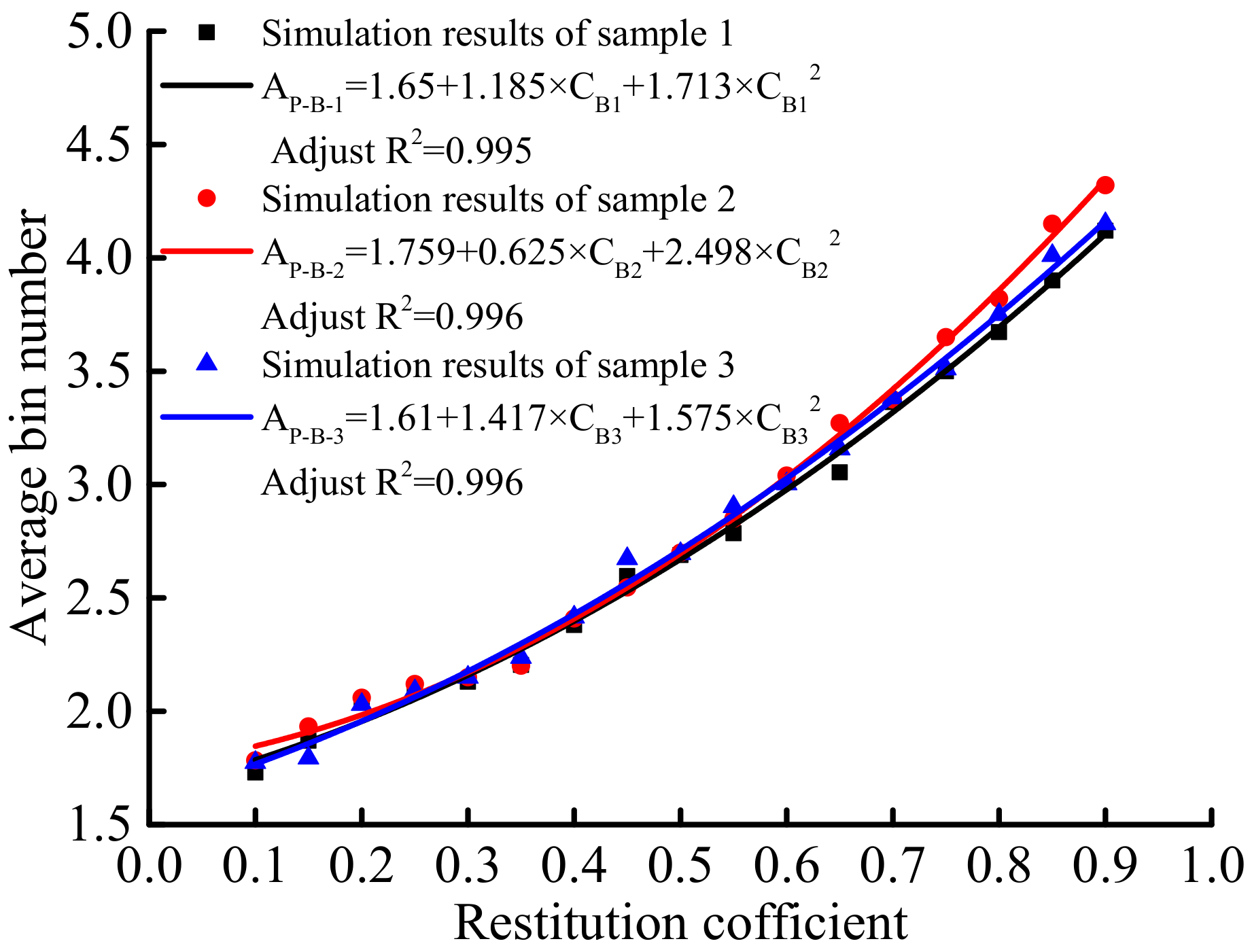
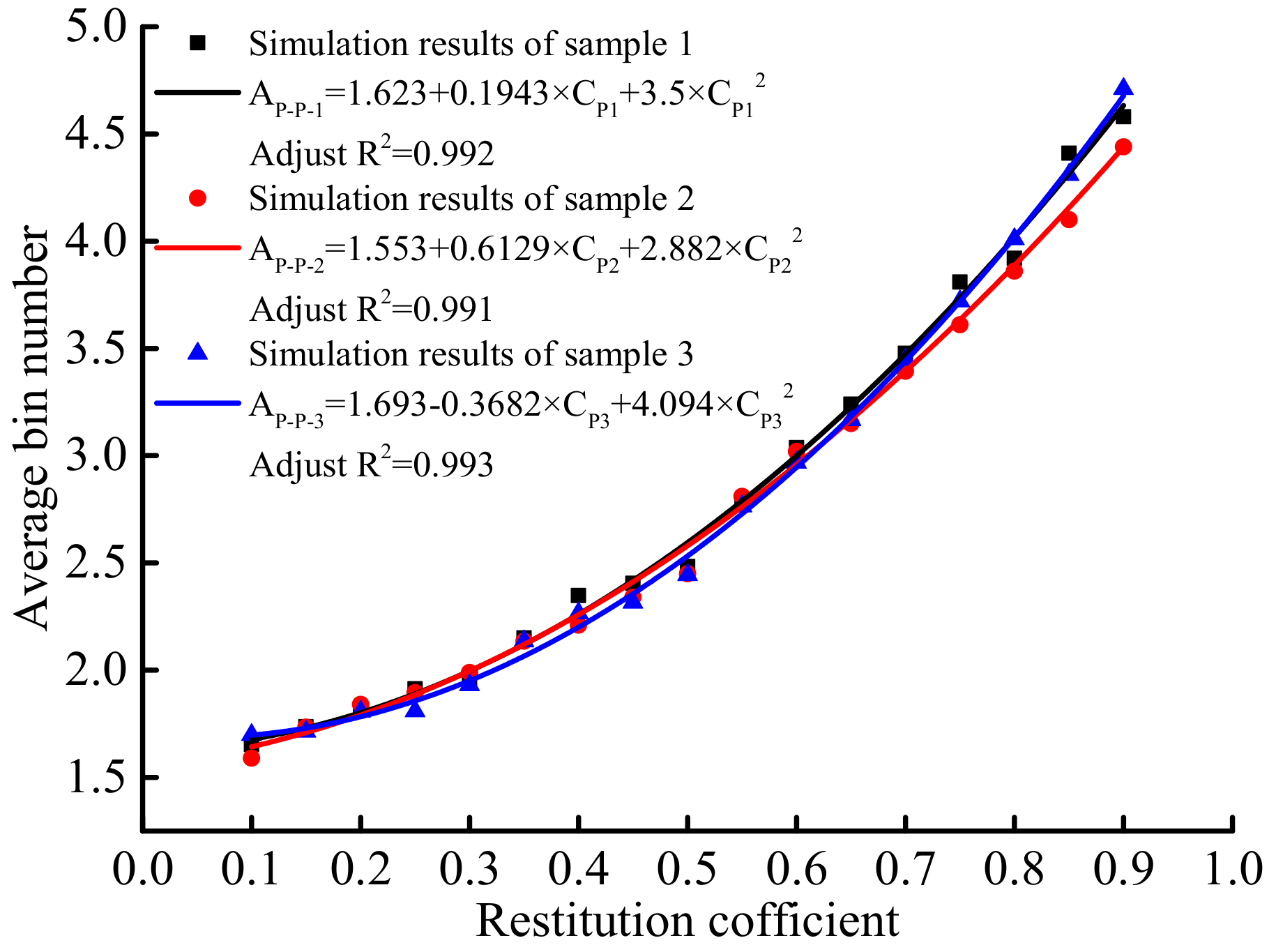
2.3.2. Calibration of Restitution Coefficients

The geometry of the experimental device duplicated that used in the simulation of the inclined surface drop, and the schematic diagram is shown in Figure 6. A virtual circular surface consistent with the particle releasing pipe in terms of diameter (20 mm) was established to generate particles in Rocky DEM. The particles were generated continuously, and the generation rate was 0.005 kg/s, the generation time was 23 s, and the total number of particles was 300. A flat plate was used to replace the bottom plate of the quartz sand to improve the simulation efficiency, and the restitution coefficient from particle to bottom plate was set to the minimum value of 0.1. The simulation duration and output frequency were 30 s and 0.01 s, respectively. The pre-simulation results showed that the particle would not rebound after falling on the bottom plate, indicating that the parameters were reasonable. After the simulation finished, the number of maize kernels in each bin was recorded, and the average bin number was calculated using Equation (1).

The relationship between the restitution coefficient and the average bin number was explored through the single factor test, and the regression equation between the average bin number and the restitution coefficient (C) was established using Matlab. The average bin number of measured values was substituted into the regression equation to determine the restitution coefficient. In the calibration process, the particle to particle and particle to low carbon steel restitution coefficients were both set to 0.10–0.90, with an increment of 0.05 [1].

2.3.3. Calibration of the Friction Coefficients

As shown in Figure 7a, the geometry and testing conditions used in the experimental test setup were duplicated in the DEM simulations. A virtual circular surface consistent with the upper end funnel in terms of diameter (100 mm) was established to generate particles in the Rocky DEM. The particles were generated continuously, and the generation rate was 0.45 kg/s, the generation time was 1 s, and the total mass of particles was 0.45 kg. The simulation duration and output frequency were 3 s and 0.001 s, respectively. After finishing the simulation, the AoR of the maize kernel models shown in Figure 7b and the discharging process were recorded in Rocky DEM.

The contact parameters were demonstrated to affect the AoR and discharging time. Specifically, these were the particle to particle static friction coefficient (pps), the dynamic friction coefficient (ppd), the restitution coefficient (C_P), the particle to low carbon steel static friction coefficient (pbs), the dynamic friction coefficient (pbd), and the restitution coefficient (C_B). The two-level factorial design, the response surface methodology, and the numerical optimization in Design Expert 12.0 were used to calibrate the friction coefficients. The two-level factorial design was used to screen the major parameters that significantly influence the AoR and discharging time. In this test design, the above mentioned factors were set to two levels. Referring to the relevant literature [1,9,31], the threshold and levels of the contact parameters were designed as shown in

Table 4. Factors and levels of the two-level factor design.

Factor Level	pps	ppd	CP	pbs	pbd	CB
−1	0.1	0.1	0.1	0.1	0.2	0.3
+1	0.5	0.4	0.6	0.4	0.5	0.8

. The response surface methodology based on central composite design (CCD) was used to analyze the influence law of major factors on indexes, and the numerical optimization was used to determine the optimal values of major factors to bring the indexes closer to the target value.

3. Results and Discussion

3.1. Restitution Coefficient Calibration

Figure 8 and Figure 9 show the average bin number of simulation results varied with the restitution coefficients of p–p and p–w. The average bin number increased as the restitution coefficient increased, which corresponds with Kingsly Ambrose’s conclusion [6], indicating that the simulation was reliable. Furthermore, the average bin number of each sample of maize kernels differed, although the restitution coefficient was the same. In order to ensure the accuracy of the restitution coefficient when applying the regression equation, the simulation results of each sample of maize kernels were used to perform a regression analysis by Matlab to determine the regression equation of the average bin number and the restitution coefficient, as shown in Figure 8 and Figure 9. The adjustment R² values of the regression equations were all higher than 0.99, indicating an excellent fitting effect.

In the regression equations, A_P-B-n represents the average bin number when the maize kernels of the n^th sample collided with the low carbon steel plate, where n = 1, 2, 3, with the units being pieces. C_B-n is the restitution coefficient of maize kernels of the nth sample contacting the low-carbon steel plate. A_P–P-n is the average bin number of collisions between maize kernels in the nth sample. C_P-n is the restitution coefficient between maize kernels of the nth sample.

The average bin numbers obtained from the experiments in Section 1.1 were substituted into the regression equations to determine the restitution coefficients, as shown in

Table 5. The results for the maize kernel restitution coefficients.

No. Sample	AP-B	CB	AP–P	CP
Sample 1	3.91	0.856	2.86	0.567
Sample 2	3.80	0.789	2.75	0.547
Sample 3	3.55	0.750	2.55	0.505

. The restitution coefficient decreased as the moisture content of maize kernels increased, and the particle to low-carbon steel plate restitution coefficient was higher than that of the particle to particle restitution coefficient. The results show that the energy loss during the collision between maize kernels and the low-carbon steel plate was lower than that during the collision between maize kernels, which corresponds to Yan Hui’s conclusion [39], indicating that the simulation was reliable.

3.2. Parameter Calibration of the Friction Coefficient

3.2.1. Two-Level Factorial Design

The two-level factorial test scheme and simulation results for Sample 2 are shown in

Table 6. The scheme and results of the two-level factor test.

No.	Contact Parameters						AoR/(°)	Discharging Time/(ms)
	pps	ppd	CP	Pbs	pbd	CB
1	0.1	0.4	0.1	0.1	0.5	0.8	32.18	2540
2	0.1	0.4	0.6	0.1	0.2	0.3	32.00	2620
3	0.1	0.1	0.1	0.1	0.2	0.3	14.25	1765
4	0.5	0.1	0.1	0.1	0.5	0.3	20.43	2063
5	0.5	0.4	0.6	0.1	0.5	0.3	31.68	2700
6	0.5	0.1	0.6	0.4	0.2	0.3	16.07	1820
7	0.5	0.1	0.1	0.4	0.5	0.8	25.24	2020
8	0.5	0.4	0.6	0.4	0.5	0.8	38.50	2630
9	0.1	0.1	0.1	0.4	0.2	0.8	10.43	1810
10	0.1	0.1	0.6	0.4	0.5	0.3	20.63	2076
11	0.5	0.1	0.6	0.1	0.2	0.8	11.00	1775
12	0.5	0.4	0.1	0.1	0.2	0.8	28.82	2530
13	0.1	0.4	0.6	0.4	0.2	0.8	25.71	2440
14	0.1	0.4	0.1	0.4	0.5	0.3	32.01	2560
15	0.5	0.4	0.1	0.4	0.2	0.3	35.29	2590
16	0.1	0.1	0.6	0.1	0.5	0.8	19.27	2175

and

Table 7. Parameter significance determined by the analysis of variance.

Source	AoR				Discharging Time
	Coefficient Estimate	Mean Square	F-Value	p-Value	Coefficient Estimate	Mean Square	F-Value	p-Value
Model	-	177.55	15.07	<0.01	-	2.95 × 105	31.28	<0.01
X1: pps	1.28	26.41	2.24	0.17	8.88	1260.25	0.13	0.72
X2: ppd	7.43	883.06	74.96	<0.01	319.13	1.63 × 106	172.63	<0.01
X3: CP	−0.25	0.90	0.08	0.79	22.38	8010.25	0.85	0.38
X4: pbs	0.89	12.70	1.08	0.33	−13.87	3080.25	0.33	0.58
X5: pbd	2.90	134.36	11.40	<0.01	88.38	1.25 × 105	13.24	<0.01
X6: CB	−0.70	7.86	0.67	0.44	−17.12	4692.25	0.50	0.50

shows the results of the variance analysis on the simulation results as well as the significance results for each simulation parameter. It can be seen from Table 7 that the ppd and pbd (p < 0.01) have very significant influences on the AoR and discharging time of the simulation, and the effects of the other parameters (p > 0.05) on the AoR and discharging time of the simulation results were found to be very small. Therefore, only the significant parameters of the ppd and pbd were considered in the subsequent response surface experiments. The restitution coefficients of non-significant factors were set in accordance with Table 5. The contact parameters were calibrated for a future crushing simulation of the hammer mill. Since the static friction coefficients have little effect on the simulation accuracy of the crushing process, the pps and pbs were set to 0.31 [40] and 0.40 [39], respectively, by referring to the literature.

Since the results of the two-level factor analysis for all samples of maize kernels were consistent, only the simulation results and analysis of variance results of sample 2 are listed in this paper.

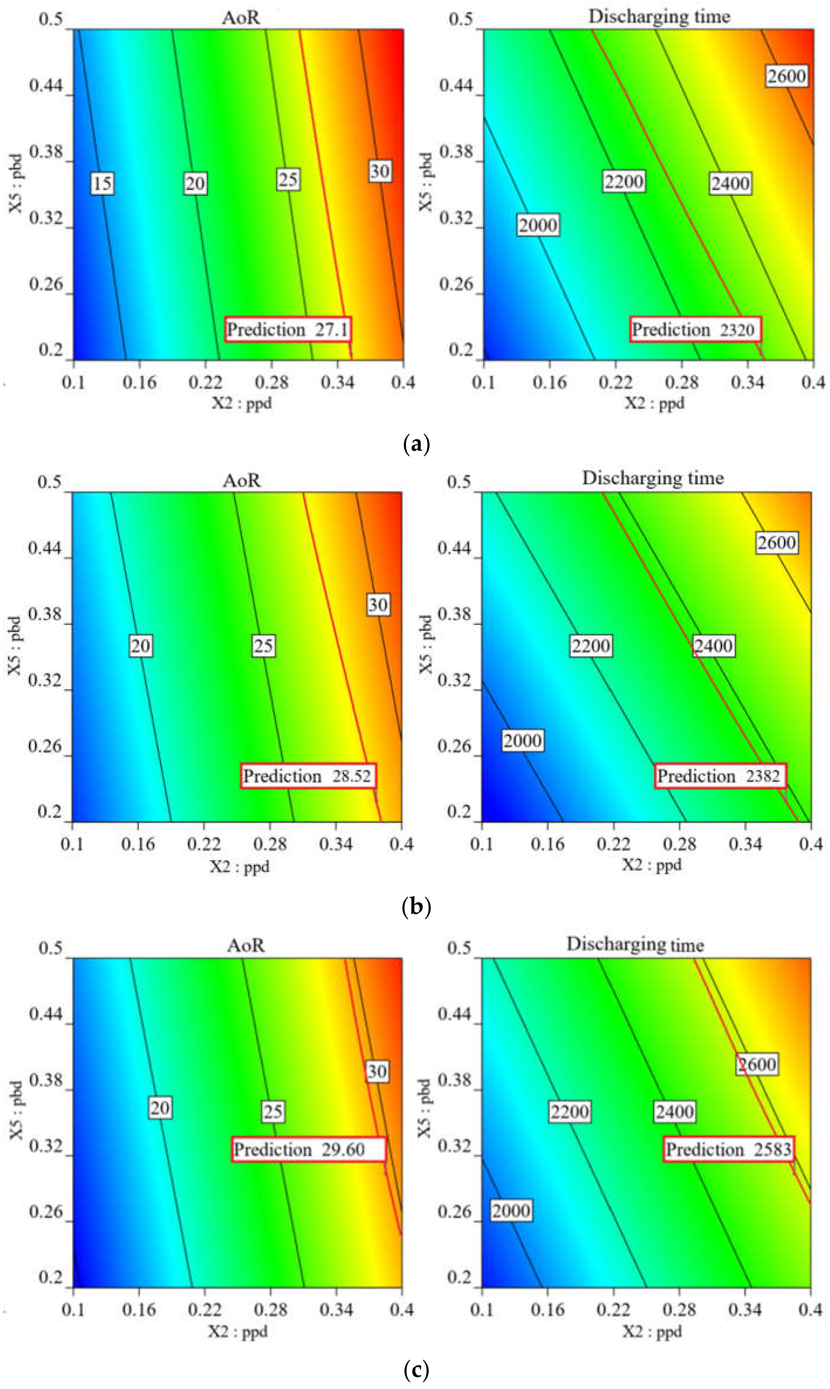
3.2.2. Response Surface Methodology Analysis

According to the results of the two-level factorial test, the ppd and pbd were taken as factors for the response surface methodology test. A two factor and three level response surface methodology test was designed. The test scheme and simulation results are shown in

Table 8. The scheme and results related to the response surface design.

No.	Factor Levels		Simulation Results
	X2: ppd	X5: pbd	Sample 1		Sample 2		Sample 3
			AoR/(°)	Discharging Time/(ms)	AoR/(°)	Discharging Time/(ms)	AoR/(°)	Discharging Time/(ms)
1	0.40	0.20	31.165	2485	29.950	2376	29.610	2400
2	0.10	0.50	17.045	2065	19.510	2143	17.870	2150
3	0.10	0.20	12.000	1766	15.100	1895	14.945	1863
4	0.25	0.35	21.540	2214	24.010	2231	23.720	2315
5	0.10	0.35	12.975	1956	18.330	1975	15.910	2052
6	0.25	0.20	20.170	2106	22.170	2251	21.610	2345
7	0.25	0.50	21.900	2435	22.825	2495	23.920	2438
8	0.40	0.50	32.010	2716	32.300	2816	32.740	2900
9	0.40	0.35	31.885	2461	31.010	2430	30.430	2648

and

Table 9. The analysis of variance of the AoR and discharging time for the response surface linear model.

	Sample 1				Sample 2				Sample 3
Source	AoR		Discharging Time		AoR		Discharging Time		AoR		Discharging Time
	F	P	F	P	F	P	F	P	F	P	F	P
Model	118.37	<0.01	112.39	<0.01	88.49	<0.01	33.69	<0.01	550.36	<0.01	44.46	<0.01
X2: ppd	231.95	<0.01	185.78	<0.01	171.17	<0.01	50.46	<0.01	1062.42	<0.01	72.98	<0.01
X5: pbd	4.79	0.07	38.99	<0.01	5.79	0.05	16.93	<0.01	38.30	<0.01	15.94	<0.01

shows the variance of AoR and the analysis of the discharging time of the response surface linear model. It can be seen from Table 9 that the linear model p-value was less than 0.01, which proves that the model is reliable. The ppd and pbd were shown to have significant impacts on the AoR and discharging time, and a subsequent analysis of the ppd and pbd was carried out.

The contours of the AoR and discharging time were determined as functions of ppd and pbd for the three samples of maize kernels based on the results of the response surface methodology analysis and are shown in Figure 10. As with increases the values of ppd and pbd, the AoR and discharging time gradually increased. Because larger ppd and pbd values are associated with greater relative movement resistance between particles and the contact surface, the AoR and the discharging time will increase accordingly.

According to Table 2, contour lines were drawn using the AoR and discharging time from the experiment results and are shown as red lines in Figure 10 when a single index (AoR or discharging time) was used for parameter calibration (for example, when calibrating the parameters of ppd and pbd, only the AoR was selected as the index). It can be seen from Figure 10 that the combinations of ppd and pbd consistent with the points on the contour lines of the AoR will be the results of parameter calibration, and it is obvious that there can be many groups of calibrated ppd and pbd combinations. However, the ppd and pbd of each granular material should be unique both in simulation and in reality. Therefore, the accuracy of parameter calibration will be reduced when only a single response value is used to calibrate ppd and pbd. This conclusion is consistent with Wensrich C.M’s research results [26].

Based on the above analysis, the AoR and discharging time were considered together to calibrate the ppd and pbd. The numerical optimization was employed to solve ppd and pbd. The solution process involved taking the experiment results for the AoR and discharging time of each sample of maize kernels and the thresholds of ppd and pbd as the constraints and then solving the values of ppd and pbd using the numerical optimization.

Table 10. Constraints and solutions for dynamic friction coefficients.

Name	Sample 1		Sample 2		Sample 3
	Constraints	Solutions	Constraints	Solutions	Constraints	Solutions
X2: ppd	0.1–0.4	0.352	0.1–0.4	0.377	0.1–0.4	0.385
X5: pbd	0.2–0.5	0.206	0.2–0.5	0.220	0.2–0.5	0.304
AOR/(°)	27.10	-	28.52	-	29.60	-
Discharging time/(ms)	2320	-	2382	-	2583	-
Desirability	-	1	-	1		1

shows the solutions to ppd and pbd, and a unique solution can be obtained for ppd and pbd for each sample of maize kernels. Meanwhile, the desirability of these solutions was calculated to be 1, indicating that the calibrating method is reliable. The results show that it is feasible to calibrate the ppd and pbd with the AoR and discharging time as indexes using the funnel method, and this can improve the accuracy and reliability of parameter calibration.

3.3. Test Validation

The accuracy of the DEM simulation, measured as the closeness of DEM results to experimental values, should be evaluated by an accredited criterion. The relative error was used as a criterion for the assessment of a simulation’s accuracy [26]. The relative error measures the accuracy of a DEM simulation using the difference between the results of a simulation (S) and an experiment (E). The relative error was calculated with Equation (3):

$$P_{error}=\frac{\left|E-S\right|}{E}\times 100\%$$

(3)

where P_error is the relative error, and E and S are the measured and simulated values, respectively.

3.3.1. Verification of Restitution Coefficients

The accuracy and reliability of the calibrated restitution coefficients should be verified with a new series of experimental results. For this purpose, the experimental results of the inclined surface drop test for 300, 400, and 500 maize kernels were compared with the results of the calibrated DEM simulation [26].

Table 11. Relative error between simulation and experiment values of the average bin number for maize kernels.

Sample	Number of Particles	Particle-Low-Carbon Steel Plate			Particle-Particle
		Experiment	Simulation	Percentage Error/(%)	Experiment	Simulation	Percentage Error/(%)
	300	3.91 ± 0.038	3.85	1.53	2.86 ± 0.033	2.92	2.09
Sample 1	400	4.01 ± 0.035	3.96	1.25	2.93 ± 0.036	2.85	2.73
	500	3.87 ± 0.039	3.95	2.10	2.84 ± 0.029	2.80	1.41
	300	3.80 ± 0.026	3.70	2.63	2.75 ± 0.035	2.79	0.36
Sample 2	400	3.85 ± 0.031	3.89	1.04	2.72 ± 0.036	2.68	1.48
	500	3.81 ± 0.024	3.90	2.36	2.80 ± 0.039	2.72	2.86
	300	3.55 ± 0.028	3.62	1.97	2.55 ± 0.027	2.60	1.96
Sample 3	400	3.60 ± 0.032	3.54	1.67	2.51 ± 0.042	2.40	4.38
	500	3.53 ± 0.038	3.61	2.27	2.49 ± 0.031	2.58	3.61

illustrates the comparisons between the experimental and simulation results of the average bin number for different amounts of maize kernels. The maximal relative errors of the average bin number of the particle to low-carbon steel plate and particle to particle were, respectively, 2.63% and 4.38%, which verifies the accuracy of the DEM simulation and the reliability of the calibrated method [6].

3.3.2. Verification of Dynamic Friction Coefficients

The accuracy and reliability of the calibrated dynamic friction coefficients should be verified by a new series of experimental results. For this purpose, the experimental results of the funnel test for maize kernel quantities of 0.45 kg, 0.60 kg, and 0.90 kg were compared with the results of the calibrated DEM simulation [26].

Table 12. Verification of the calibration of the AoR and discharging time.

Sample	Particle Mass/(kg)	AoR/(°)			Discharging Time/(ms)
		Experiment	Simulation	Relative Error/(%)	Experiment	Simulation	Relative Error/(%)
Sample 1	0.45	27.10 ± 0.86	28.31	4.46	2320 ± 35.51	2320	0.00
	0.60	27.50 ± 1.36	28.56	3.85	3240 ± 39.74	3120	3.70
	0.90	28.01 ± 1.43	28.69	2.43	4200 ± 62.03	4465	6.31
Sample 2	0.45	28.52 ± 1.26	28.61	0.32	2382 ± 29.33	2410	1.18
	0.60	28.69 ± 1.51	29.47	2.72	3200 ± 68.49	3330	4.06
	0.90	28.93 ± 1.46	29.57	2.21	4253 ± 48.03	4550	6.98
Sample 3	0.45	29.60 ± 1.07	30.67	3.61	2583 ± 42.84	2732	5.76
	0.60	30.05 ± 1.22	31.4	4.49	3690 ± 45.21	3650	1.08
	0.90	30.23 ± 1.03	31.89	5.49	5600 ± 59.33	5483	2.09

shows comparisons between the experimental and simulation results for the AoR and the discharging time for different amounts of maize kernels. The maximal relative errors of the AoR and discharging time were, respectively, 5.49% and 6.98%, which also verifies the accuracy of the DEM results and the reliability of the calibrated method.

3.4. Limitations of the Study

In the inclined surface drop experiment and the funnel experiments, maize kernels with similar structures and sizes were selected for the experiments, but maize kernel models of unified structure and size were used to complete the simulation in this study. Because the flow characteristics of the particles are impacted by their size and shape, as well as the percentage of particles of varied sizes, this could have compromised the accuracy of the parameter calibration. Therefore, in future scientific research, the particle size and shape proportion of maize kernels in the experiment should be counted, followed by the determination of the particle size distributions and the conduction of maize kernel models of various sizes. The number of particle with various sizes will be defined in simulation according to actual particle size distributions, bringing the simulation closer to actual experiments and increasing the practical significance of the simulation.

4. Conclusions

(1)

The maize kernel model was constructed by combining 3D scanning and the section method. The relative errors of the sizes of the three axes and the volume between the particle model and the real maize kernel were 3.81% and 0.48%, respectively.

(2)

The restitution coefficients between the maize kernel and low-carbon steel plate and between maize kernels were calibrated by improving the inclined surface drop method. Moreover, the dynamic friction coefficients between the maize kernel and low-carbon steel plate and between maize kernels were calibrated using the funnel method by considering the AoR with the discharging time.

(3)

Validation tests were carried out, and the maximum relative errors between the simulated and measured values obtained with the inclined surface drop method and funnel method were 4.38% and 6.98%, respectively, which verified the feasibility and accuracy of the particle model construction and parameter calibration method.

In this study, we proposed a method for constructing a convex polyhedral particle model suitable for Rocky DEM and a calibration method to calibrate contact parameters, and then the research methods were verified which are feasible and accurate. The research method used in this study could provide support for the construction of the particle model and calibration of the contact parameters of agricultural granular materials with complex geometric structures, as well as the maize kernel model and the values of the contact parameters in this paper can provide a reference for the DEM simulation of the maize kernel crushing process to design and optimize of the impact mill.

References

1. Singh, Y.; Ravindran, V.; Wester, T. Influence of feeding coarse corn on performance, nutrient utilization, digestive tract measurements, carcass characteristics, and cecal microflora counts of broilers. Pultry Sci. 2014, 93, 607–616. [Google Scholar] [CrossRef] [PubMed]
2. Metzger, M.; Glasser, B. Simulation of the breakage of bonded agglomerates in a ball mill. Powder Technol. 2013, 237, 286–302. [Google Scholar] [CrossRef]
3. Dey, S.; Dey, S.; Das, A. Comminution features in an impact hammer mill. Powder Technol. 2013, 235, 914–920. [Google Scholar] [CrossRef]
4. Ghodki, B.; Goswami, T. DEM simulation of flow of black pepper seeds in cryogenic grinding system. J. Food Eng. 2017, 196, 36–51. [Google Scholar] [CrossRef]
5. Toneva, P.; Epple, P.; Breuer, M. Grinding in an air classifier mill—Part I: Characterisation of the one-phase flow. Powder Technol. 2011, 211, 19–27. [Google Scholar] [CrossRef]
6. Chen, Z.; Wassgren, C.; Veikle, E. Determination of material and interaction properties of maize and wheat kernels for DEM simulation. Biosyst. Eng. 2020, 195, 208–226. [Google Scholar] [CrossRef]
7. Ma, H.; Zhao, Y.; Cheng, Y. CFD-DEM modeling of rod-like particles in a fluidized bed with complex geometry. Powder Technol. 2019, 344, 673–683. [Google Scholar] [CrossRef]
8. Jiménez-Herrera, N.; Barrios, G.; Tavares, L. Comparison of breakage models in DEM in simulating impact on particle beds. Adv. Powder Technol. 2018, 29, 692–706. [Google Scholar] [CrossRef]
9. Coetzee, C.J. Review: Calibration of the discrete element method. Powder Technol. 2017, 310, 104–142. [Google Scholar] [CrossRef]
10. Chen, Y.; Cai, W.; Zou, X. Extrusion mechanical properties of fresh litchi. Trans. Chin. Soc. Agric. Eng. 2011, 27, 360–364. [Google Scholar]
11. Zhang, W.; Xie, J.; Zhang, X. Finite element analysis of mechanical properties of whole fresh jujubes. Food Sci. 2016, 37, 100–104. [Google Scholar]
12. Yang, Z.; Sun, J.; Guo, Y. Effect of moisture content on compression mechanical properties and frictional characteristics of millet grain. Trans. Chin. Soc. Agric. Eng. 2015, 31, 253–260. [Google Scholar]
13. Peng, F.; Wang, H.; Fang, F. Calibration of discrete element model parameters for pellet feed based on injected section method. Trans. Chin. Soc. Agric. Mach. 2018, 49, 140–147. [Google Scholar]
14. Wang, Y.; Liang, Z.; Zhang, D. Calibration method of contact characteristic parameters for corn seeds based on EDEM. Trans. Chin. Soc. Agric. Eng. 2016, 32, 36–42. [Google Scholar]
15. Aghajani, N.; Ansaripour, E.; Kashaninejad, M. Effect of Moisture Content on Physical Properties of Barley Seeds. J. Agric. Sci. Technol. 2011, 14, 161–172. [Google Scholar]
16. ROCKY DEM. DEM Technical Manual; Engineering Simulation and Scientific Software (ESSS): Florianópolis, Brazil, 24 January 2020. [Google Scholar]
17. Yu, Q.; Liu, Y.; Chen, X. Calibration and experiment of simulation parameters for panax notoginseng seeds based on DEM. Trans. Chin. Soc. Agric. Mach. 2020, 51, 123–132. [Google Scholar]
18. Beakawi Al-Hashemi, H.; Baghabra Al-Amoudi, O. A review on the angle of repose of granular materials. Powder Technol. 2018, 330, 397–417. [Google Scholar] [CrossRef]
19. Liu, Y.; Zong, W.; Ma, L. Determination of three-dimensional collision restitution coefficient of oil sunflower grain by high-speed photography. Trans. Chin. Soc. Agric. Eng. 2020, 36, 44–53. [Google Scholar]
20. Hou, Z.; Dai, N.; Chen, Z. Measurement and calibration of physical property parameters for agropyron seeds in a discrete element simulation. Trans. Chin. Soc. Agric. Eng. 2020, 36, 46–54. [Google Scholar]
21. Santos, D.; Barrozo, M.; Duarte, C. Investigation of particle dynamics in a rotary drum by means of experiments and numerical simulations using DEM. Adv. Powder Technol. 2016, 27, 692–703. [Google Scholar] [CrossRef]
22. Liu, W.; He, J.; Li, H. Calibration of simulation parameters for potato minituber based on EDEM. Trans. Chin. Soc. Agric. Mach. 2018, 49, 125–135. [Google Scholar]
23. Dai, F.; Song, X.; Zhao Wu, Y. Simulative Calibration on contact parameters of discrete elements for covering soil on whole plastic film mulching on double ridges. Trans. Chin. Soc. Agric. Mach. 2019, 50, 49–56. [Google Scholar]
24. Li, Y.; Li, F.; Xu, X. Parameter calibration of wheat flour for discrete element method simulation based on particle scaling. Trans. Chin. Soc. Agric. Eng. 2019, 35, 320–327. [Google Scholar]
25. Wen, X.; Yuan, H.; Wang, G. Calibration method of friction coefficient of granular fertilizer by discrete element simulation. Trans. Chin. Soc. Agric. Mach. 2020, 51, 115–122. [Google Scholar]
26. Derakhshani, S.; Schott, D.; Lodewijks, G. Micro–macro properties of quartz sand: Experimental investigation and DEM simulation. Powder Technol. 2015, 269, 127–138. [Google Scholar] [CrossRef]
27. Cao, K.; Hao, B. Modern China Feed Engineering; Shanghai Scientific and Technology Literature Press: Shanghai, China, 2014; pp. 374–462. [Google Scholar]
28. Huang, K.; Chen, X.; Chen, P. Simulation and experimental analysis of mass transfer in drying a single corn kernel. J. Eng. Thermophys. 2017, 38, 2005–2010. [Google Scholar]
29. GB 1353-2018; Maize. Standardization administration: Beijing, China, 13 July 2018.
30. JJD 264-2008; Measuring instruments for cereals density. The Central People’s Government of People’s Republic of China: Beijing, China, 23 November 2008.
31. Han, Y.; Jia, F.; Tang, Y. Influence of granular coefficient of rolling friction on accumulation characteristics. Acta Phys. Sin. 2014, 63, 173–179. [Google Scholar]
32. Barmwal, P.; Kadam, D.; Singh, K. Influence of moisture content on physical properties of maize. Int. Agrophys. 2012, 26, 331–429. [Google Scholar] [CrossRef]
33. Zhao, W. Rersearch on Combined Type of Spiral Bar Tooth Threshing Mechanism for Seed Corn. Doctoral Dissertation, Northwest A&F University, Xian, China, 1 November 2012. [Google Scholar]
34. Ma, W.; You, Y.; Wang, D. Parameter calibration of alfalfa seed discrete element model based on RSM and NSGA-II. Trans. Chin. Soc. Agric. Mach. 2020, 51, 136–144. [Google Scholar]
35. Gustafson, R.J.; Thompson, D.R.; Sokhansanj, S. Temperature and stress analysis of corn kernel—Finite Element Analysis. Trans. ASABE 1979, 22, 955–960. [Google Scholar] [CrossRef]
36. Han, D. Optimization Simulation and Experimental Research of Inside Filling Air-Blowing Maize Precision Seed-Metering Device. Doctoral Dissertation, China Agricultural University, Beijing, China, 1 June 2018. [Google Scholar]
37. Singh, S.; Finner, M.; Rohatgi, P. Structure and mechanical properties of corn kernels: A hybrid composite material. J. Mater. Sci. 1991, 26, 274–284. [Google Scholar] [CrossRef]
38. Dong, P.; Guo, Y.; Hou, J. Study on the grinding method and parameter for testing corn breakage resistance. J. Maize Sci. 2019, 27, 124–129. [Google Scholar]
39. Yan, H. A New Kind of Method for the Optimizated Design of Combination Inner-Cell Corn Precision Seed Metering Device. Doctoral Dissertation, Jilin University, Changchun, China, 1 December 2012. [Google Scholar]
40. Wang, X. A Multi-Sphere Based Modelling Method for Maize Grain Assemblies. Master Dissertation, Jilin University, Changchun, China, 1 June 2017. [Google Scholar]
Figure 1. Inclined surface drop method. (a) Experiment device (b) Schematic.
Agriculture 12 00664 g001
Figure 2. Funnel experiment device. (a) Experimental device, (b) Schematic, (c) AoR of maize kernels.
Agriculture 12 00664 g002
Figure 3. Sizes of the three axes of the maize kernel.
Agriculture 12 00664 g003
Figure 4. Maize kernel particle construction. (a) 3D scanned maize kernel; (b) contour lines; (c) multi-segment straight lines; (d) maize kernel model.
Agriculture 12 00664 g004
Figure 5. Maize kernel models with different array distances.
Agriculture 12 00664 g005
Figure 6. Simulation setup used for the inclined surface drop method.
Agriculture 12 00664 g006
Figure 7. Simulation setup used for the funnel method. (a). Simulation device; (b). AoR of the maize kernel model.
Agriculture 12 00664 g007
Figure 8. Relationship between the average bin number and the restitution coefficient of particle to low-carbon steel restitution coefficient.
Agriculture 12 00664 g008
Figure 9. Relationship between the average bin number and the particle to particle restitution coefficient.
Agriculture 12 00664 g009
Figure 10. Effects of dynamic friction coefficients on the AoR and discharging time of maize kernels. (a) Sample 1; (b) Sample 2; and (c) Sample 3 of the maize kernel models.
Agriculture 12 00664 g010