Dynamics of Temperature Variation in Soil under Fallow Tillage at Different Depths

Abstract

One of the important processes taking place during soil surface tillage is the variation of the soil temperature at different depths. The paper presents the results of research into the dynamics of soil temperature variation in terms of such parameters of the soil as its thermal diffusivity and temperature oscillation frequency. It has been established that the temperature oscillation amplitude decreases when the depth increases, following the logarithmic law. In this variation, the temperature difference between the 0–5 cm layer and the adjacent 5–10 cm layer has the greatest value. This circumstance is a favorable factor for the fallow tillage technology, where the soil is regularly cultivated to a depth of no more than 5 cm, in case of a moisture deficit. A decrease in the frequency of the soil temperature oscillations can result in the reduced level of its heating in different layers. In terms of qualitative changes, the reduction in soil thermal diffusivity results in the amplitude of the soil temperature oscillations being lowered and at the same time the maximum of these oscillations being shifted towards a delay.

1. Introduction

When the soil is loosened, the field surface in immediate contact with atmospheric air increases [1], so supporting the intensive evaporation of soil moisture [2]. This evaporation, which increases with the depth of the loosened soil layer [3], substantially changes the temperature conditions of the soil layer and consequently its properties [4,5].

First, soil temperature has a significant effect on soil carbon fixation [6,7,8]. In this respect, it has been found that with a temperature increase the CO₂ emissions from the soil into the atmosphere become greater [9,10]. For example, one of the interesting results obtained in the research is the fact that the CO₂ emissions at a soil temperature of 23 °C are greater by a factor of 2.4 than the emissions at a temperature of 10 °C [11,12,13].

The solar energy that reaches the soil surface can be split into soil heat flux, sensible heat reflection, and latent heat for water evaporation [14]. The heat flux of soil relies on its heat capacity and thermal conductivity, which are affected by bulk density, soil composition, and water content [15]. Usually, dry soils cool and warm faster than wet soils due to soil particles, which have a lower heat capacity and greater heat conductivity than water [16]. In this context, the tillage technique modifies the soil surface by increasing air pockets in which evaporation occurs, and then potentialities of soil heating and drying are changed. Tillage causes a lower soil thermal conductivity compared to that of the untilled soil and then no-tillage system promotes temperature lowering in the soil. Really, comparing to the conventional soil tillage techniques, the no-tillage allows us to reduce by at least 1.97 °C the heating of the soil [17,18]. Moreover, the temperature reduction can reach a level of over 3 °C if the no-tillage technique is joined to soil mulching, which allows us to lower the soil heat flux and increase the amount of reflected heat. Soil temperature goes down also using the strip-tillage technique, even if it remains higher by about 1.4–1.9 °C than no-tillage practices [19], considering that the strip-tillage has the feature of increasing soil temperatures along the rows and lower the temperature along the inter-rows covered by residues in which soil moisture is conserved [20,21].

Bulgakov et al. [22] developed the black fallow tillage technology, in which the soil ripping depth does not exceed 5 cm. It has been established experimentally that the CO₂ emissions from fallow soil at a temperature of 33.4 °C are 5.5 times greater than at a temperature of 17.6 °C [23]. Furthermore, no experimental data concerning the soil temperature distribution as a function of the soil tillage depth are available, and data about the temperature of the 0–5 cm soil layer are not known, nor how this temperature affects those ones concerning the deeper soil layers.

In contrast, in the fallow tillage technology such data are needed to choose the suitable tillage parameters to create negligible conditions of soil heating and, accordingly, of moisture losses from the layers below 5 cm.

The dynamics of the variation of soil temperature in relation to depth can be adequately described by a suitable mathematical model, and currently three typologies of such models are known [24,25].

The first typology is represented by the empirical models, which are the most widely used. They are based on the statistical relations between the soil temperatures at certain depths and the local climate and soil conditions. These conditions include radiation absorbed at the soil surface, soil surface emissivity, air volumetric heat capacity, soil surface conductivity, air temperature, air density, atmospheric pressure, latent heat for water vaporization, water vapor pressure at the surface, air vapor pressure, soil thermal conductivity, soil surface albedo, and others.

The second typology is represented by the mechanical models, which are based on the rather complicated balance of radiant energy. Additionally, such models attempt to describe the apparent, latent, and heat-conducting heat flows in the soil, which are partially described by the Fourier-Biot equation [25].

The models in the third typology allow us to calculate the temperature in different soil layers based on the physical principles of heat flows [26]. However, the boundary temperature at the soil surface must be found empirically in such models.

The deeper analysis of the models of all typologies highlights their complexity for being employed in practice.

Taking into account the aforesaid, the aim of this research is to find a mathematical tool which would be simple for calculation purposes but at the same time would enable the process of heat penetration into soil to be controlled. The results of the analysis would be useful for carrying out the fallow tillage technology, which affects a worked soil depth of no more than 5 cm.

2. Materials and Methods

2.1. The Considered Mathematical Model

One of the possible theoretical solutions of the Fourier-Biot equation has been assumed as quite a simple model, for analyzing the law T ($h_s$, t), concerning the distribution of the soil temperature t, °C, along its tillage depth $h_s$, cm [27]:

$$T\left(h_s,t\right)=T_s+A_o·\left[sin\left(\omega t-h_s·\sqrt{\frac{\omega }{2k}}\right)\right]·exp\left(-h_s·\sqrt{\frac{\omega }{2k}}\right),$$

(1)

where $T_s, A_o$ are, respectively, the mean value and amplitude of the soil surface temperature, °C; $\omega$ is the soil surface temperature oscillation frequency, h^–1; k is the thermal diffusivity of the soil, cm² h^–1.

No data has been found on how adequately this equation represents the real dynamics of the $T=f\left(h_s,t\right)$ process that takes place in some specific soil conditions. Furthermore, there is no data on the effect that the period or frequency of the soil temperature oscillations and especially the thermal diffusivity k of the soil have on the distribution of the temperatures in the soil layers.

Therefore, first of all, in order to verify the adequacy of the assumed mathematical model, that is Equation (1), experimental tests were carried out to assess the agreement among the effective temperatures measured over a time period in the 0–5 cm layer and the corresponding values calculated by means of Equation (1).

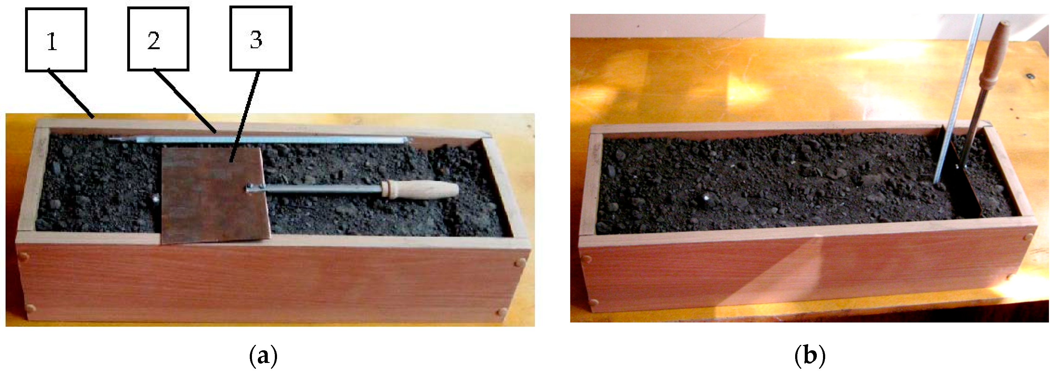
2.2. Laboratory and Field Test Carried Out to Verify the Adequacy of the Mathematical Model

The measurements were carried out in a fallow field in Zaporizhia Oblast (Ukraine), the soil of which had the following characteristics: dark chestnut, medium loam soil with a humus content of 2.6% in the 0–20 cm layer. The same layer contained (per kg of soil): (i) 21.2 mg of total nitrogen; (ii) 38.5 mg of phosphorus; and (iii) 295.0 mg of potassium. The minimum moisture-holding capacity of the soil was at a level of 21–22%, its withering point −9%.

The soil temperature in the 0–5 cm layer was measured over a period of three spring days (from 28 to 30 of May 2021), by using the DS18B20 (Dallas Semiconductor) sensor. This tool had the following main characteristics: a temperature range of –10 °C to +85 °C, and an absolute measurement error of less than 0.5%. The electric signal from the sensor was recorded with the use of an Arduino Uno device.

The soil thermal diffusivity k was assessed by the copper plate method. This copper plate had the following dimensions: (i) thickness, 0.2 cm; (ii) width, 15 cm; (iii) height, 10 cm (Figure 1). The plate was heated to a temperature of 60 °C. This temperature was measured by means of the HYELEC MS6501 digital thermometer equipped with a Type K thermocouple and characterized by a measurement error of less than 2 °C. The heated copper plate was immersed in the soil (Figure 1) and in turn placed in a box with the following dimensions: (i) length, 50 cm; (ii) width, 16 cm; and (iii) depth, 15 cm.

A mercury thermometer TM-10 (Figure 1a) with a division value of 0.2 °C was placed at a distance of $X=3$ cm from the plate centerline. In the course of time, the temperature of the soil at the point situated at a distance of $X=3$ cm from the centerline gradually rose, reached the maximum value $T_{max}$, stayed at this maximum level over a time $T_i$ (s), then went down.

The readings of the mercury thermometer were recorded each 60 s. The number of experiments for determining the thermal diffusivity of the soil (k) was equal to 5. The value of the coefficient k in each experiment was calculated using the following formula:

$$k=\frac{1800·X^2}{\left(T_{max}+0.5·T_i\right)}$$

(2)

where X was the distance between copper plate and thermometer, cm; $T_{max}$ was the time between the measuring start and the time corresponding to the maximum temperature recorded by the thermometer, s; $T_i$ was the duration of the time, over which the thermometer has registered the temperature $T_{max}$.

Prior to conducting the experiments, the moisture content and density of the soil were measured. The moisture content was determined with the use of the gravimetric (thermostat-weight) technique [28].

The soil bulk density was measured as follows [29]. A soil sample was taken with a 28.35 cm³ cylinder and weighed on the scales. The latter were configured to measure in ounces. Because $1 \mathrm{oz}.=28.35 \mathrm{g}$, the scale displayed the value of the soil mass that was equal to its density in g cm^–3.

The parameters $T_s, A_o$, and ω in Equation (1) needed for verifying its adequacy were found by analyzing the soil temperature measurements obtained over a three-day period specifically in the 0–5 cm layer.

The soil surface temperature values calculated by means of Equation (1) were compared with the experimental temperature values measured through the aforementioned DS18B20 electronic transducer over a three-day period. The calculated and experimental data agreement pattern was used to estimate the adequacy of Equation (1).

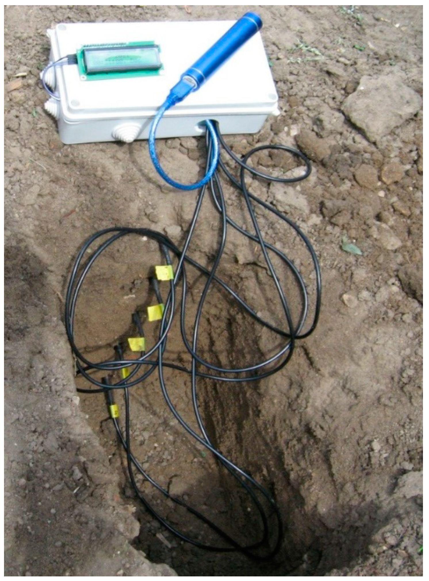
2.3. Experimental Test Aimed at Measuring the Soil Temperature Distribution along the Depth

The experimental investigations were carried out in the soil with the parameters described earlier in the paper. The soil background within the depth range of 0–25 cm was divided into 5 layers, each 5 cm thick. In each layer, a DS18B20 temperature sensor was placed (Figure 2), then soil was filled in to cover the sensors.

The signals from the soil temperature sensors were recorded in a text file in the memory card with the use of the Arduino Uno unit. The resultant experimental data were used to plot the respective relation diagrams.

The distribution of the soil temperature in the 0–25 cm layer was recorded in the period from 1 to 3 of June 2021.

3. Results and Discussion

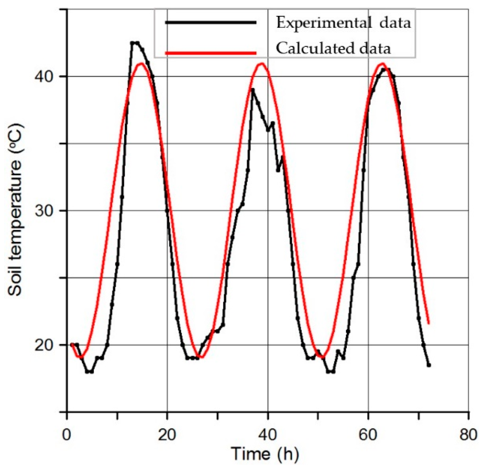
3.1. Adequacy of the Mathematica Model

As a result of processing the obtained experimental data with the use of empirical Equation (2), it has been established that the soil under investigation with a moisture content of 14.5% and a bulk density of 1.23 g cm^–3 has a thermal diffusivity coefficient of k = 18.0 cm² h^–1.

Based on the data obtained for the soil temperature dynamics in the 0–5 cm layer (Figure 3), the following values have been assumed for the purpose of verifying the adequacy of Equation (1): T_s = 30 °C; A_o = 11 °C; ω = 0.25 rad h^–1.

The comparison of the calculated and experimental data (Figure 3) has proved that the maximum difference between them within the whole range of the recorded measurements does not exceed 20%. Such a result provides reasonable grounds to consider Equation (1) as adequate and suitable mathematical model for the further predictive analysis of the patterns in the distribution of the soil temperature along the depth.

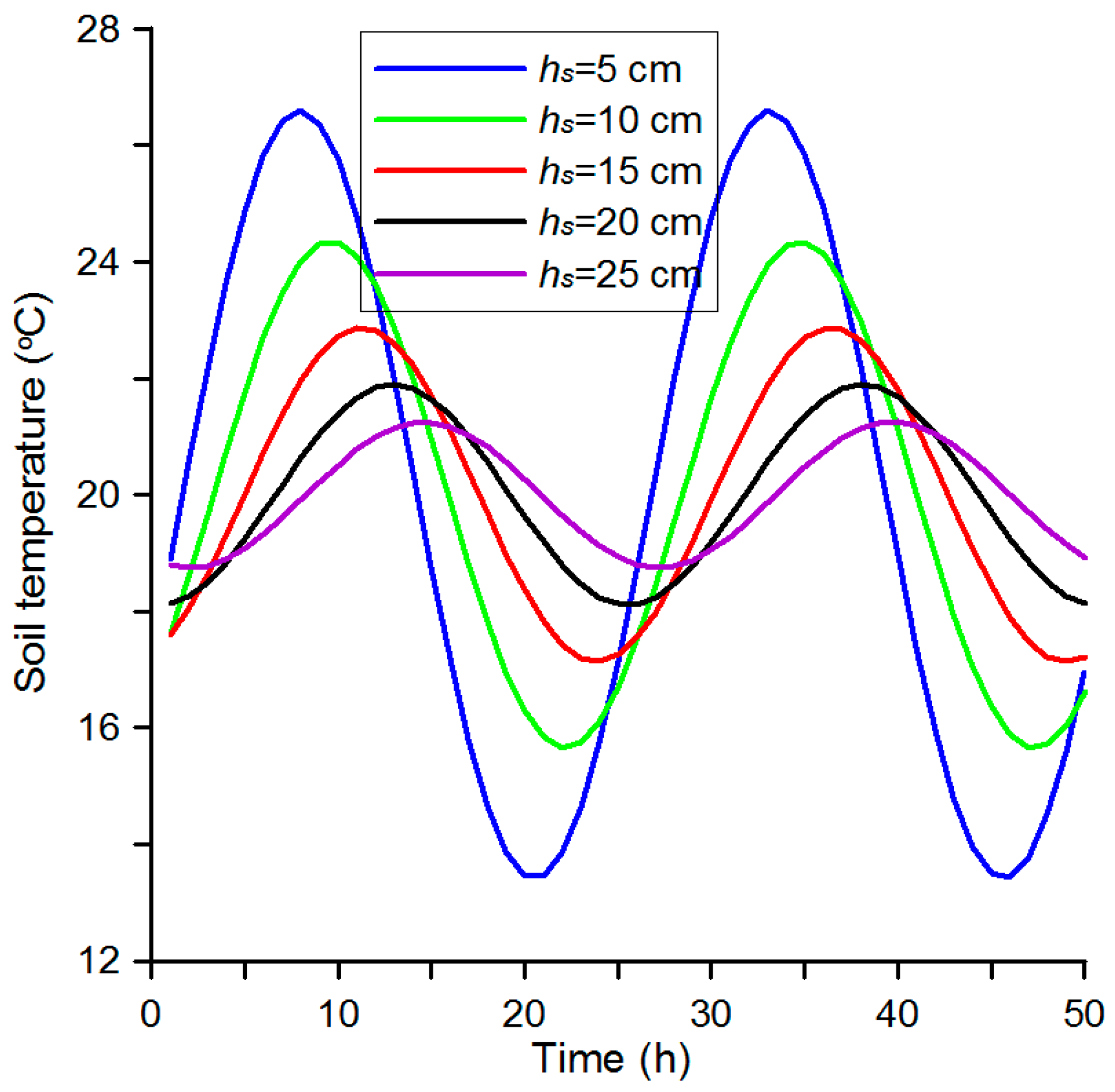
3.2. Analysis of the Heat Penetration into the Soil through the Mathematical Model

Some examples of the dynamics of soil temperature variation at different depths, obtained by means of Equation (1), are reported in Figure 4. Their analysis indicates the following: the deeper in the soil the point of observation is, the smaller the temperature T oscillation amplitude becomes. In principle, this conclusion agrees in a qualitative sense with the data presented in the papers by Horton et al. [19], Arkhangelskaya [30], and Sándor and Fodor [25].

It is to be pointed out that the decrease in temperature with time (t) is not proportional, but follows the logarithmic law (Figure 5), which can be satisfactorily approximated by the following equation:

$$T=7.774·\ln \left(t\right)+42.451.$$

(3)

According to this law, the difference of temperatures between the 5 cm and 10 cm layers is greater than that between the 10 cm and 15 cm layers. On the other hand, the soil temperature difference between the 10 cm and 15 cm layers is smaller than between the 15 cm and 20 cm layers. In the case under consideration, for example, the difference between the maximum temperature values in the 5 cm and 10 cm layers is equal to 2.3 °C. The same difference between the 10 cm and 15 cm layers is equal to 1.3 °C, i.e., by 1 °C lower.

It is to be pointed out that such a trend in the dynamics of the soil temperature variation with the depth is very important for the fallow tillage technology. As mentioned previously, one of its features is the systematic cultivation of the soil to a depth of no more than 5–6 cm. In that context, if the soil temperature difference between the 0–5 cm and 5–10 cm layers is greater than between the 5–10 cm and 10–15 cm layers, the conditions arise for obtaining dew in the soil at the boundary between the 0–5 and 5–10 cm layers.

Therefore, Equation (1) provides the theoretical basis to solve the problem of finding the dew point in the soil. In the conditions of a soil moisture deficit, this problem is of critical importance.

Figure 4 highlights that the decrease in the soil temperature oscillation amplitude at greater depths is accompanied by a certain phase shift Δt of the temperature towards a delay with respect to the surface. Theoretically this time lag Δt can be calculated by the following formula [30]:

$$\mathsf{\Delta }t=\frac{h_s}{2}·\sqrt{\frac{T_t}{\pi k},}$$

(4)

where $T_t$ is the temperature oscillation period, h.

In the case under consideration $T_t=\frac{2\pi }{\omega }=\frac{6.28}{0.25}=25.12 \mathrm{h}$, therefore, the phase shift Δt (that is, the delay) in the temperature oscillations shown in Figure 4 is equal to 1.75 h.

In terms of reducing the level of soil heating, it is desirable that the parameter $\mathsf{\Delta }t$ shows a growing trend. It can be concluded from Equation (5) that this purpose can be achieved in three different ways: (i) by increasing the temperature oscillation period $T_t$ (or reducing the frequency ω); (ii) by reducing the value of the thermal diffusivity k of the soil; (iii) by simultaneously changing the parameters $T_t$ and k.

The calculations based on Equation (1) indicate (Figure 6) that the decrease in the soil temperature oscillation frequency at a depth of 5 cm from 0.25 to 0.15 rad h^–1 quite expectedly results in the increased value of the oscillation period $T_t$. In the case under consideration, it is equal to approximately 3 h.

At the same time, simultaneously with the increase in the soil temperature oscillation period, certain growth is observed in the maximum values of the temperature. According to the calculations based on Equation (1), in the case of a decrease in ω from 0.25 to 0.15 rad h^–1, this growth will be small and equal to a mere 0.6 °C (Figure 6).

It should be noted that such a parameter as the soil temperature oscillation frequency can be controlled only in indoor rooms, such as greenhouses [31]. In outdoor areas, the value of the parameter ω is determined only by the present climatic conditions.

As distinct from ω, the value of the thermal diffusivity k of the soil can be controlled. The analysis of the calculated data obtained on the basis of Equation (1) proves that the reduction in the value of the coefficient k from 28 to 8 cm² h^–1 results in a decrease in the soil temperature oscillation amplitude with the simultaneous shift of the temperature maximum towards a delay (Figure 7). The amount of this shift is about 1 h, while the difference between the maximum values of the soil temperature reaches 2 °C in this case.

The next step is to find out in what way it is possible in practice to change (in the case under consideration—to decrease) the value of the thermal diffusivity of the soil k.

According to Arkhangelskaya [30], Goncharov and Shein [27]:

$$k=\frac{\lambda }{C_s·\rho },$$

(5)

where λ, $C_s$, ρ are the heat conductivity factor, the specific heat capacity, and the density of the soil, respectively.

The analysis of Equation (5) results in the conclusion that greater soil density values correspond to lower heat conductivity values and vice versa. The bulk density of the soil can be changed by means of tillage, i.e., loosening it.

In the fallow tillage technology that implies the soil tillage to a depth of no more than 5 cm, the density of this layer is always lower as compared to the density of the 5–10 cm layer and then the thermal diffusivity of the soil in the first layer is higher, than in the second one. Due to the higher value of the coefficient k, the soil in the 0–5 cm layer is heated to a greater extent, than the soil in the 5–10 cm layer. Due to this situation, when the ambient air passes through the 0–5 cm soil layer, its high thermal potential changes little. Passing further into the soil, the warm air contacts the more compacted, denser and, therefore, cooler soil in the 5–10 cm layer. As a result of that, there is a potential possibility that, at the interface between the 0–5 cm and 5–10 cm layers, such a difference between the soil temperatures arises that it occurs the condensation and dew. As aforesaid, such a result is very desirable in the conditions of a soil moisture deficit.

The right application of Equation (1) then can contribute to assessing and solving conditions of intra-soil moisture deficit.

3.3. Analysis of the Heat Penetration into the Soil through the Mathematical Model

Such an approach is rather efficient in terms of its practical application because the use of the similar data obtained experimentally (Figure 8) is less convenient.

The actual dynamics of temperature variations along the soil depth shown in Figure 8 highlight similar trends to the theoretical temperature distributions of Figure 4, calculated using Equation (1).

However, Figure 8 is not convenient for the objective assessment of the discussed process. First of all, because the real dynamics of the temperature variation along the depth can be, as in this case, unsteady in terms of the mathematical expectation. The difficulty in this situation is that the pattern of this instability is virtually impossible to predict.

Furthermore, the plotted temperature curves can feature certain data trends (like the curve for the 0–5 cm soil layer, Figure 8), the cause of which is very difficult to explain and even more so to predict. The theoretical data are in such cases more suitable for both the analysis and the further forecasting.

4. Conclusions

It has been established in the research that the amplitude of the soil temperature oscillations decreases with an increase in the depth. This decrease follows the logarithmic law so that the temperature difference between the 0–5 cm layer and the interfacing 5–10 cm layer has the greatest value. That is a favorable factor for the application of the fallow tillage technology in the conditions of a moisture deficit since this technology implies the systematic cultivation of the soil to a depth of no more than 5 cm.

The reduction in the frequency (or the increase in the period) of the soil temperature oscillations can result in the decrease in the level of soil heating across the layers. The growth of the maximum temperature value in each soil layer that is possible in this case is not significant. This conclusion is rather informative for the controlled greenhouse conditions.

In terms of qualitative changes, a decrease in the value of the thermal diffusivity of the soil k results in the reduced amplitude of the soil temperature oscillations and simultaneously the shift of the maximum of these oscillations towards a time delay. In quantitative terms, when the value of the parameter k decreases by a factor of 3.5 (from 28 to 8 cm² h^–1), the value of the time delay is equal to about 1 h, while the difference between the maximum soil temperature values reaches 2 °C.

References

1. Bulgakov, V.; Pascuzzi, S.; Adamchuk, V.; Ivanovs, S.; Pylypaka, S. A theoretical study of the limit path of the movement of a layer of soil along the plough mouldboard. Soil Tillage Res. 2019, 195, 104406. [Google Scholar] [CrossRef]
2. Lehnert, M. The Soil Temperature Regime in the Urban and Suburban Landscapes of Olomouc, Czech Republic. Morav. Geogr. Rep. 2013, 21, 27–36. [Google Scholar] [CrossRef] [Green Version]
3. Adamchuk, V.; Bulgakov, V.; Nadykto, V.; Ivanovs, S. Investigation of tillage depth of black fallow impact upon moisture evaporation intensity. Eng. Rural Dev. 2020, 377–383. [Google Scholar] [CrossRef]
4. Onwuka, B.M. Effects of soil temperature on some soil properties and plant growth. Adv. Plants Agric. Res. 2018, 8, 34–37. [Google Scholar] [CrossRef]
5. Pascuzzi, S.; Santoro, F. Analysis of the Almond Harvesting and Hulling Mechanization Process: A Case Study. Agriculture 2017, 7, 100. [Google Scholar] [CrossRef] [Green Version]
6. Norman, J.M.; Garcia, R.; Verma, S.B. Soil surface CO2 fluxes and the carbon budget of a grassland. J. Geophys. Res. 1992, 97, 18845–18853. [Google Scholar] [CrossRef]
7. Lou, Y.; Li, Z.; Zhang, T. Carbon dioxide flux in a subtropical agricultural soil of China. Water Air Soil Pollut. 2003, 149, 281–293. [Google Scholar] [CrossRef]
8. Bilandžija, D.; Zgorelec, Ž.; Kisić, I. The influence of agroclimatic factors on soil CO2 emissions. Coll. Antropol. 2014, 38, 77–83. [Google Scholar]
9. Jabro, J.D.; Sainju, U.; Stevens, W.B.; Vans, R.G. Carbon dioxide flux as affected by tillage and irrigation in soil converted from perennial forages to annual crops. J. Environ. Manag. 2008, 88, 1478–1484. [Google Scholar] [CrossRef]
10. Pascuzzi, S.; Anifantis, A.S.; Blanco, I.; Scarascia Mugnozza, G. Hazards assessment and technical actions due to the production of pressured hydrogen within a pilot photovoltaic-electrolyzer-fuel cell power system for agricultural equipment. J. Agric. Eng. 2016, 47, 88–93. [Google Scholar] [CrossRef] [Green Version]
11. Moore, T.R.; Dalva, M. Methane and carbon dioxide exchange potentials of peat soils in aerobic and anaerobic laboratory incubations. Soil Biol. Biochem. 1997, 29, 1157–1164. [Google Scholar] [CrossRef]
12. Almagro, M.; Lopez, J.; Querejeta, J.I.; Martinez-Mena, M. Temperature dependence of soil CO2 efflux is strongly modulated by seasonal patterns of moisture availability in a Mediterranean ecosystem. Soil Biol. Biochem. 2009, 41, 594–605. [Google Scholar] [CrossRef]
13. Júnior, N.L.; Simas, F.N.B.; Mendon, E.D.S.; Souza, J.V.; Panosso, A.R.; Schaefer, C.E.; Gilkes, R.J.; Prakonkep, N. Spatial and temporal variability of soil C-CO2 emissions and its relation with soil temperature in King George Island, Maritime Antarctica. Polar Sci. 2010, 4, 479–487. [Google Scholar] [CrossRef] [Green Version]
14. Sun, X.; Li, S.; Du, H. The Influence of Corn Straw Mulching on Soil Moisture, Temperature and Organic Matter. J. Biobased Mater. Bioenergy 2017, 11, 662–665. [Google Scholar] [CrossRef]
15. Bulgakov, V.; Pascuzzi, S.; Adamchuk, V.; Kuvachov, V.; Nozdrovicky, L. Theoretical Study of Transverse Offsets of Wide Span Tractor Working Implements and Their Influence on Damage to Row Crops. Agriculture 2019, 9, 144. [Google Scholar] [CrossRef] [Green Version]
16. Licht, M.A.; Al-Kaisi, M. Strip-tillage effect on seedbed soil temperature and other soil physical properties. Soil Tillage Res. 2005, 80, 233–249. [Google Scholar] [CrossRef]
17. Ramakrishna, A.; Tam, H.M.; Wani, S.P.; Long, T.D. Effect of mulch on soil temperature, moisture, weed infestation and yield of groundnut in northern Vietnam. Field Crop. Res. 2006, 95, 115–125. [Google Scholar] [CrossRef] [Green Version]
18. Ochsner, T.E.; Horton, R.; Ren, T. A New Perspective on Soil Thermal Properties. Soil Sci. Soc. Am. J. 2001, 65, 1641–1647. [Google Scholar] [CrossRef]
19. Abu-Hamdeh, N.H. Thermal properties of soils as affected by density and water content. Biosyst. Eng. 2003, 86, 97–102. [Google Scholar] [CrossRef]
20. Horton, R.; Bristow, K.L.; Kluitenberg, G.J.; Sauer, T.J.; Horton, R.; Kluitenberg, G.J. Crop Residue Effects on Surface Radiation and Energy Balance-Review Crop Residue Effects on Surface Radiation and Energy Balance-Review. Theor. Appl. Climatol. 1996, 54, 27–37. [Google Scholar] [CrossRef] [Green Version]
21. Dahiya, R.; Ingwersen, J.; Streck, T. The effect of mulching and tillage on the water and temperature regimes of a loess soil: Experimental findings and modeling. Soil Tillage Res. 2007, 96, 52–63. [Google Scholar] [CrossRef]
22. Bulgakov, V.; Nadykto, V.; Kaminskiy, V.; Ruzhylo, Z.; Volskyi, V.; Olt, J. Experimental research into the effect operating speed on uniformity of cultivation depth during tillage in fallow field. Agron. Res. 2020, 18, 1962–1972. [Google Scholar] [CrossRef]
23. Galic, M.; Bilandzija, D.; Percin, A.; Sestak, I.; Mesic, M.; Blazinkov, M.; Zgorelec, Z. Effects of agricultural practices on carbon emission and soil health. J. Sustain. Dev. Energy Water Environ. Syst. 2019, 7, 539–552. [Google Scholar] [CrossRef]
24. Luo, Y.; Loomis, R.S.; Hsiao, T.C. Simulation of soil temperature in crops. Agric. For. Meteorol. 1992, 61, 23–38. [Google Scholar] [CrossRef]
25. Sándor, R.; Fodor, N. Simulation of soil temperature dynamics with models using different concepts. Sci. World J. 2012, 2012, 590287. [Google Scholar] [CrossRef] [Green Version]
26. Li, R.; Ma, J.; Sun, X.; Guo, X.; Zheng, L. Simulation of Soil Water and Heat Flow under Plastic Mulching and Different Ridge Patterns. Agriculture 2021, 11, 1099. [Google Scholar] [CrossRef]
27. Goncharov, V.M.; Shein, E.V. Agrophisics; Feniks Editor: Rostov-na-Dony, Russia, 2006; ISBN 978-5222077412. (In Russian) [Google Scholar]
28. Bulgakov, V.; Pascuzzi, S.; Nadykto, V.; Ivanovs, S.; Adamchuk, V. Experimental study of the implement-and-tractor aggregate used for laying tracks of permanent traffic lanes inside controlled traffic farming systems. Soil Tillage Res. 2021, 208, 104895. [Google Scholar] [CrossRef]
29. Bulgakov, V.; Pascuzzi, S.; Ivanovs, S.; Nadykto, V.; Nowak, J. Kinematic discrepancy between driving wheels evaluated for a modular traction device. Biosyst. Eng. 2020, 196, 88–96. [Google Scholar] [CrossRef]
30. Arkhangelskaya, T.A. Temperature Regime of Complex Soilscape; GEOC: Moskow, Russia, 2012; (In Russian). [Google Scholar] [CrossRef]
31. Baldoin, C.; Balsari, P.; Cerruto, E.; Pascuzzi, S.; Raffaelli, M. Improvement in Pesticide Application on Greenhouse Crops: Results of a Survey about Greenhouse Structures in Italy. Acta Hortic. 2008, 801, 609–614. [Google Scholar] [CrossRef]
Figure 1. Complete set of equipment for measuring thermal diffusivity of soil (a) and arrangement of this equipment during measurements (b): 1—box with soil; 2—thermometer; 3—copper plate.
Agriculture 12 00450 g001
Figure 2. Soil temperature measurement sensors placed at different depths.
Agriculture 12 00450 g002
Figure 3. Experimental and calculated data on soil temperature variation.
Agriculture 12 00450 g003
Figure 4. Dynamics of soil temperature variation at different depths according to Equation (1).
Agriculture 12 00450 g004
Figure 5. Dynamics of soil temperature decrease with time.
Agriculture 12 00450 g005
Figure 6. Dynamics of soil temperature variation in relation to temperature oscillation frequency at a depth of 5 cm.
Agriculture 12 00450 g006
Figure 7. Dynamics of soil temperature variation at a depth of 5 cm at different values of thermal diffusivity of soil.
Agriculture 12 00450 g007
Figure 8. Dynamics of soil temperature variation at different depths observed in field conditions.
Agriculture 12 00450 g008
Publisher’s Note: MDPI stays neutral with regard to jurisdictional claims in published maps and institutional affiliations.