Article

Analysis on Regional Differences and Spatial Convergence of Digital Village Development Level: Theory and Evidence from China

1
School of Economics and Management, Yantai University, Yantai 264500, China
2
College of Economics and Management, Northwest Agriculture and Forestry University, Yangling 712100, China
*
Author to whom correspondence should be addressed.
Agriculture 2022, 12(2), 164; https://doi.org/10.3390/agriculture12020164
Submission received: 21 November 2021 / Revised: 17 January 2022 / Accepted: 21 January 2022 / Published: 24 January 2022
(This article belongs to the Special Issue Agricultural Food Marketing, Economics and Policies)

Abstract

:
In the context of the rapid development of the global Internet, evaluating the digital village development level (DVI) in different regions is important for policy formulation and scientific research in the field of rural digital development. Based on the measurement of DVI using panel data of provinces from 2005 to 2018, we also explored the causes of DVI development differences using the Dagum Gini coefficient decomposition and spatial convergence method. The study found that: (1) During the whole sample period, the DVI in China and the four major regions showed a significant upward trend as a whole, with the highest in the eastern region and the lowest in the western region, but the development of DVI among different provinces showed regional non-equilibrium characteristics. (2) DVI has a typical agglomeration effect in the spatial and geographical distribution, and regional differences are the primary source of differences in DVI development in China, but the overall regional differences show a decreasing trend. (3) Except for the northeast region, σ -convergence exists in the other three regions; in addition, all regions have significant conditional β -convergence, but the convergence speed is significantly different. (4) Rural population density, industrial structure, and economic development level significantly affect DVI. Therefore, we suggest strengthening the inter-regional connection and element flow and realizing the improvement of the overall DVI of the region through cooperation and mutual assistance.

1. Introduction

Digital information technology with the Internet as the core has gradually transformed into new production factors and governance tools, becoming an important driving force for the current high-quality economic development and a vital support force for building a modern social governance system [1,2,3]. According to the China Internet Development Report 2019, as of June 2019, the number of Internet users in rural China has reached 225 million. The Internet penetration rate in rural areas is about 46%. To further utilize the critical role of digital information technology in agricultural and rural economic and social development, the national government departments also issued relevant policy documents to guide its development. However, in practice, the construction of a digital village provides new ideas and new opportunities for rural development in various regions [4]. However, due to the large gap in resource endowment, information infrastructure, and economic development among different regions in China, there is a significant gap in the development level of digital villages in the various areas [5]. Therefore, research on the dynamic changes of the digital rural development level in different regions of China and revealing the regional differences, sources, and convergence characteristics of the digital rural development level in different regions was necessary.
There is also apparent heterogeneity in the development of digital villages in different countries worldwide. The U.S. Department of Agriculture’s Office of Rural Development announced a series of policies for rural construction and financial support to help rural American communities improve their economy and quality of life. The United States adopted the Advanced Wireless Research Platform project to explore different delivery models of rural broadband and implement innovative solutions such as precision agriculture [6]. The Indian government has recently formulated a plan called “Digital Village” to provide free WIFI service to Indian villages, which will further promote the cashless payment mode in villages [7]. Cornwall is at the forefront of the U.K.’s rural digitization strategy, implementing innovative measures such as broadband access, digital training, community digital centers, and e-health, and introducing the most advanced technologies such as V.R. and virtual reality activities to narrow the digital divide [8]. In order to solve the challenges of out-migration in rural areas, the Finnish government has researched “smart villages” for many years. Digital services are considered the foundation for maintaining a vibrant village, and the main measures include digital education, e-health, telecommuting, and digital training [9]. As far as the concept of the digital village is concerned, some scholars have determined that safety, security, well-being, and happiness are some of the parameters of the digital village [10], and Visvizi and Lytras [11] pointed out that it can learn from the research of the smart city and equalize it. The research on the land application is carried out at the micro-level of villages, which can provide ideas for the study of digital villages. In the European Commission document, digital villages and smart villages are defined as rural areas, and communities that build on their existing strengths and assets, as well as new opportunities to develop added value and where traditional and new networks are enhanced using digital communications technologies, innovations, and the better use of knowledge for the benefit of inhabitants [12]. We mainly refer to the official policy documents of the Chinese government and the practice of rural development and believe that DVI refers to the development of rural areas relying on the digital economy, with modern information networks as an essential carrier, and digital technology innovation as the core driving force for rural development.
The construction of a digital village is a new growth highlight of China’s rural areas in the future, so the digital village’s theoretical cognition and practical exploration have become a hot spot of academic and industry research [13,14]. Many scholars have carried out multi-dimensional research on the digital villages from an interdisciplinary perspective, but there is no unified measurement standard for measuring DVI. Shen et al. [15] through combing the micro informatization indicators of rural residents, constructed a micro measurement model of the digital village from the aspects of the use of information equipment, the acquisition and utilization of information demand, and the information public service, and measured the level of DVI by using the entropy weight method; Zhang et al. [16] constructed a digital village macro-environment, infrastructure support, information environment, government environment, and application of the environment five dimensions of the evaluation index system, to measure the development level of digital villages in China’s 31 provinces and autonomous regions from 2013 to 2017; Fang [17] constructed the evaluation index system of digital rural development from the perspective of rural development, and selected seven dimensions, including scientific and technological agriculture, smart farmers, digital economy, network government affairs, intelligent environment, modern medical and welfare, and digital infrastructure.
All of these have significant reference values for this study. However, there are still some deficiencies: the digital village development level measurement will have considerable differences due to the different angles and emphasis of the index system selection, and scholars have not reached a consensus. The applicability of other measurement methods is extensive, resulting in differences in the measurement results. Most of the existing studies on digital villages remain theoretical. There is no systematic study on the regional differences, spatial distribution, and stochastic convergence of digital villages in China. The literature on the development of this digital village discusses many indicators, including digitization, intelligence, and the Internet, but lacks scientific papers or more studies to confirm it. The development of smart villages or digital villages is one of the critical issues to be considered in sustainable development and the overall development of society in the future. In this paper, we construct a comprehensive index system covering multiple levels to measure the level of digital villages and discuss the aspects of spatial heterogeneity and driving factors, aiming to provide information for developing countries on a larger scale in the world. The national development of digital villages and smart villages provides feasible ideas, which will only discuss how to build smart villages at the theoretical level and expand to more detailed aspects to help other regions more accurately make up for the shortcomings of digital village development.

2. Materials and Methods

2.1. Data Source

This paper adopts provincial panel data, including 434 research samples from 31 provinces in mainland China from 2005 to 2018. The main reason for selecting these data is the absence of data from Hong Kong, Macau, and Taiwan provinces, so we only decided on data from 31 provinces in mainland China for the analysis. The data used are from the China Statistical Yearbook, China Population, and Employment Statistical Yearbook, etc. However, in practice, China’s Statistical Yearbook data may be missing or omitted for many provinces in China due to differences in economic development and the level of statistical capacity in each region. We mainly adopted the linear interpolation method to deal with the missing data. Because China’s geographic location spans three major geographical segments [18], China is divided into four regions according to the classification of the China Statistical Yearbook [19]: the eastern region, the central region, the western region, and the northeastern region (Figure 1). The eastern region includes Beijing, Tianjin, Hebei, Shanghai, Jiangsu, Zhejiang, Fujian, Shandong, Guangdong, and Hainan; the central region includes Shanxi, Anhui, Jiangxi, Henan, Hubei, and Hunan provinces; the western region includes inner Mongolia, Guangxi, Chongqing, Sichuan, Guizhou, Yunnan, Tibet, Shaanxi, Gansu, Qinghai, Ningxia, and Xinjiang; and the northeastern region includes Liaoning, Jilin, and Heilongjiang. In practical terms, there are significant differences in the level of economic development, natural resource status, and geographic climate in these four regions. Our analysis of DVI from the four regions can explain them from a regional distribution perspective.

2.2. Methods

2.2.1. Construction and Evaluation Method of DVI

The Evaluation Index System of DVI

How to evaluate DVI scientifically is very important to understand the real situation of digital village development in China [20,21]. Ranade et al. [22] stated that digital villages or smart villages should be based on the local conditions, infrastructure, available resources in the rural area, and local demand, as well as the potential export of goods to urban areas. Some scholars also point out that digital villages should be defined according to the concept of digital cities, and their digital villages should contain economic components, environmental components, and social components, covering various aspects such as broadband, clean technology, and social life [23]. The study by Guo and Chen [24] argues that digital villages should be based on modern information networks, and the main components cover village industry digitalization, intellectual data, life data, and three other essential aspects. All of the above studies have explored the concept of the digital village, which mainly contains parts such as digital information technology facilities and the Internet development environment. However, as far as digital village development is concerned, the residents within the village are the main subjects and practitioners of the village [25,26], so the development of the digital village must consider the digital technology level and economic development ability of the residents within the village. Therefore, in addition to the digital village infrastructure and information environment indicators from existing studies, we added the indicator of digital main development ability that can reflect village residents’ economic capacity and digital technology level. We have constructed the evaluation index system of digital village development, which includes 15 indicators in three dimensions: main development ability, infrastructure construction, and information environment (Table 1). The main development ability is selected from the income, consumption, and education level of rural residents. The infrastructure construction is selected from the aspects of line laying, broadband business development, and agricultural machinery. The information environment is selected from the Internet penetration rate and rural residents’ digital equipment ownership.

The Value of the DVI Evaluation Method

We used the entropy method comprehensive evaluation model to measure the comprehensive DVI in China and four major regions from 2005 to 2018. To reduce and avoid the subjective factors and some objective limitations in the process of weight determination, we used the entropy weight method to weigh the indicators and then used the weighted sum method to measure and evaluate the development level of digital village areas [27,28]. The advantage of this method compared with other methods is that the entropy method can overcome the randomness and conjecture problems that cannot be avoided by the subjective weighting method and can effectively solve the problem of information overlap among multi-index variables [29,30]. The specific steps are as follows:
All indicators are dimensionless. Among them, the positive index that Equation (1) below can express it:
X i j = x i j min { x 1 j , , x n j } max { x 1 j , , x n j } min { x 1 j , , x n j }
The negative indicator using Equation (2):
X i j = max { x 1 j , , x n j } x i j max { x 1 j , , x n j } min { x 1 j , , x n j }
where x i j is the original index value of the j - th index of the evaluation object i , and n is the number of evaluation objects.
The construction formula of a normalized matrix p i j using Equation (3):
p i j = X i j i = 1 n X i j
Calculate the entropy of the j - th index using Equation (4):
e j = k i = 1 n p i j ln p i j
where k = 1 ln n > 0 .
Calculate the redundancy of information entropy using Equation (5):
d j = 1 e j
Calculate the weight of the index relative to its dimension using Equation (6):
w j = d j j = 1 m k d j
where k is the dimension, k max = 5 , m k is the number of corresponding dimension indicators.
Finally, the calculation formula of the comprehensive DVI using Equation (7):
S i = j = 1 m k w j p i j

2.2.2. Decomposition of Dagum Gini Coefficient

The Dagum Gini coefficient decomposition method was used to decompose the regional differences of DVI in eastern, central, western, and northeastern China (Dagum, 1997). According to the decomposition method of the Gini coefficient proposed by Dagum, the total Gini coefficient is calculated using Equation (8):
G = j = 1 k h = 1 k i = 1 n j r = 1 n h | y j i y h r | / 2 n 2 y ¯
where, y j i ( y h r ) is the comprehensive index of the digital rural development of provinces in region j ( h ); y ¯ is the average value of the digital rural development index; n is the number of provinces; k is the number of regions; n j ( n h ) is the number of provinces in region j ( h ); G is the overall Gini coefficient; j and h are different provinces in k regions, j = 1, 2, …; k, i, r is the different province in region j ( h ).
Dagum [31] decomposes the overall Gini coefficient G into the contribution of differences within regions G w , the contribution of difference between regions G n b , and the contribution of trans variation intensity G t , the relationship among them are G = G w + G n b + G t ; Equations (9) and (10) respectively represent the Gini coefficient G j j of a certain region (such as j region) and the Gini coefficient of inter-regional (j and h regions) G j h :
G j j = 1 2 y ¯ j i = 1 n j r = 1 n j | y j i y j r | n j 2
G j h = i = 1 n j r = 1 n j | y j i y j r | n j n h ( y ¯ j + y ¯ h )
G w = j = 1 k G j j p j s j
G n b = j = 2 k h = 1 j 1 G j h ( p j s h + p h s j ) D j h
G t = j = 2 k h = 1 j 1 G j h ( p j s h + p h s j ) ( 1 D j h )
where, in Equations (11)–(13), p j = n j / n is the ratio of the number of provinces in region j to the total number of provinces in China; s j = n j y ¯ j / n y ¯ , j = 1 , 2 , , k ; D j h is the relative influence of the level of DVI between region i and region j using Equation (14):
D j h = d i h p j h d i h + p j h
where, the calculation formulas of d j h and p j h are shown in Equations (15) and (16), d j h is defined as the difference of DVI among regions, representing the mathematical expectation of the sum of all sample values satisfying y j i y h r > 0 condition in j region and h region; p j h is defined as the hyper variant first moment, representing the mathematical expectation of the sum of y h r y j i > 0 sample values in j region and h region; F j ( F h ) represents the cumulative density distribution function of region j. The Equation is:
d j h = 0 d F j ( y ) 0 y ( y x ) d F h ( x )
p j h = 0 d F h ( y ) 0 y ( y x ) d F j ( x )

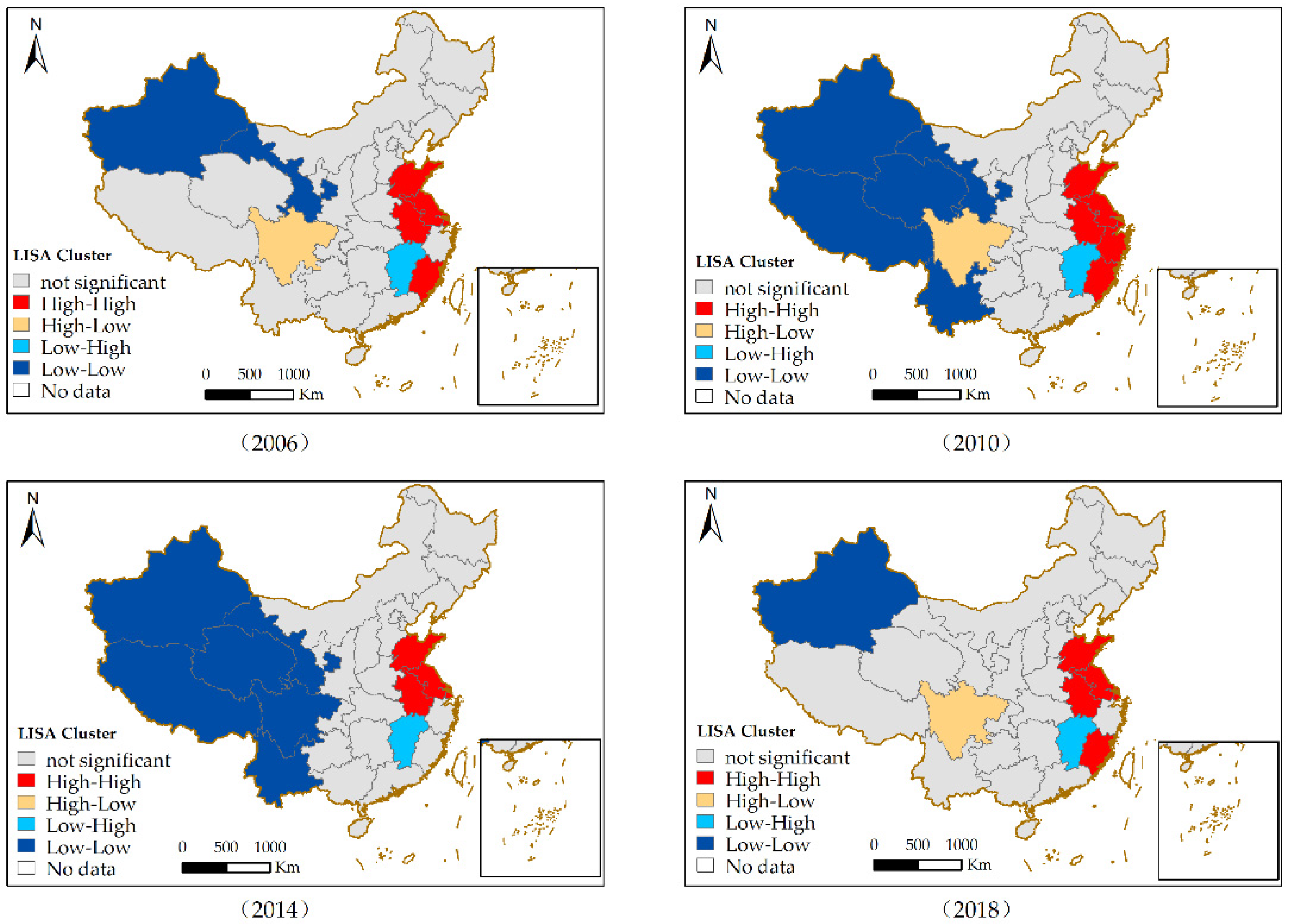
2.2.3. Spatial Autocorrelation Analysis

The spatial autocorrelation analysis includes global spatial autocorrelation and local spatial autocorrelation [32]. Global spatial autocorrelation mainly tests the general trend of spatial correlation of adjacent or similar regional unit attribute values in the whole study area [33,34]. Moran’s I index is generally used to measure spatial correlation [35]. The calculation equation is as follows:
I = i = 1 n j = 1 n W i j ( x i x ¯ ) ( x j x ¯ ) S 2 i = 1 n j = 1 n W i j
where, I is Moran’s I index; n is the number of research objects; x i ,   x j represent the attribute values of spatial units i and j; W i j is the spatial weight matrix; S 2 is the variance of the observation value; x ¯ is the average value of the observation value. The value of I is between −1 and 1 [36]. I > 0 is a spatial positive correlation. When I < 0 is a spatial negative correlation, the smaller the value, the stronger the degree of negative correlation. I = 0 represents spatial uncorrelation. Global spatial autocorrelation can reflect the distribution pattern of the research object in the whole regional space, but cannot obtain the location of the research object cluster region [37,38,39].
The four quadrants of local Moran’s I and the Moran scatter plot correspond to four different types of local association, namely HH (high-high), HL (high-low), LH (low-high), and LL (low-low) [40,41]. Among them, HH and LL indicate that adjacent provinces have a positive spatial correlation, provinces with a high or low degree of DVI have a spatial agglomeration effect; HL and LH indicate that there is a spatial negative correlation between adjacent provinces, provinces with a high (low) DVI are surrounded by provinces with a low (high) DVI.

2.2.4. Spatial Convergence Model

The convergence model was used to measure the convergence or difference of the income gap. Then it was applied to many fields such as economic growth, innovation efficiency, and so on [42,43]. σ -convergence and β -convergence are standard methods for convergence analysis [3]. β -convergence includes absolute β -convergence and conditional β -convergence [44]; after adding the spatial effect, it can be divided into the β -convergence spatial autoregressive model (SAR) and spatial error model (SEM) [45].

σ -Convergence Model

σ -convergence is an intuitive understanding of the concept of convergence [46]. If the difference of DVI among provinces was reduced, then there is σ -convergence, otherwise, there is no σ -convergence. In this paper, the variation coefficient of DVI of each province after logarithmic processing was used to reflect the change trend of the gap.
σ = i N j ( Y i j Y ¯ i j ) 2 / N j Y ¯ i j
where j represents each region (j = 1, 2, 3, 4); i represents the provinces in each region (i = 1, 2, 3, …); and Ni represents the number of provinces in each region; Y ¯ i j is the average DVI of region j.

β -Convergent Spatial Autoregressive Model (SAR)

The traditional absolute β -convergence model is ln Y i , t + 1 ln Y i t = α I + β ln Y i t + ε , after considering the influence of spatial effect, a spatial autoregressive model with absolute β -convergence is established [47,48,49]:
ln Y i , t + 1 ln Y i t = α I + β ln Y i t + ρ W ( ln Y i , t + 1 ln Y i t ) + ε
where, i represents the provinces included in the sample, and Y i t represents DVI of i province in the t year, ln Y i , t + 1 ln Y i t represents the logarithmic growth of DVI of the i province in the t year, I is the spatial unit vector, W is the spatial weight matrix, and α and β are the corresponding parameters to be estimated. Among them, β is the convergence coefficient. If β > 0 is statistically significant, it indicates that the DVI in China has divergent characteristics, On the contrary, if β < 0 , it means that there is absolute β -convergence in the DVI of China, and the convergence rate is λ = ( 1 / T ) × ln ( 1 | β | ) . ρ represents the spatial autoregressive coefficient.
The conditional β -convergence is different from the absolute β -convergence, which admits differences in economic characteristics and steady-state values among provinces [50,51]. As learned from the Gotway et al. [52] study, based on the absolute β -convergence spatial autoregressive model and the relevant control variables, the conditional β -convergence spatial autoregressive model can be obtained:
ln Y i , t + 1 ln Y i t = α I + β ln Y i t + ρ W ( ln Y i , t + 1 ln Y i t ) + ξ μ i t + ε
where, μ i t represents the selected control variable, and ξ represents the coefficient of the control variable, reflecting the influence degree and direction of the chosen control variable on the growth rate of DVI; if β < 0 passes the significance test, then the spatial conditional β -convergence has existed, otherwise, there is no spatial conditional β -convergence.

Spatial Error Model with β -Convergence (SEM)

Different from the β -convergence spatial autoregressive model (SAR), in the β -convergence spatial error model (SEM), the spatial correlation of individual provinces is caused by random disturbance [53]. Therefore, the spatial error model with absolute β -convergence can be expressed as follows:
ln Y i , t + 1 ln Y i t = α I + β ln Y i t + ε
ε = λ W ε 0 + μ
where, ε is the random disturbance term, and λ is the influence of the random disturbance term of DVI of other provinces on the growth rate of DVI in this province. Similar to the spatial autoregressive model with β -convergence, when β < 0 is statistically significant, it means that the growth rate of the digital village developed areas is less than that of the backward areas, and there is absolute β -convergence; otherwise, there is no such convergence. When λ < 0 is statistically significant, it means that the random disturbance of other provinces will have a negative impact on the growth rate of the DVI of i province and there is a negative spatial effect. By adding a control term to the absolute β -convergence spatial error model, the conditional β -convergence spatial error model can be obtained:
ln Y i , t + 1 ln Y i t = α I + β ln Y i t + ξ μ i t + ε
ε = λ W ε 0 + μ
where, μ i t is the selected control variable, ξ is the coefficient of the control variable, reflecting the influence degree and direction of the selected control variable on the growth rate of DVI. If β < 0 passes the significance test, it shows that there exists conditional β -convergence, otherwise, there is no conditional β -convergence.

3. Results

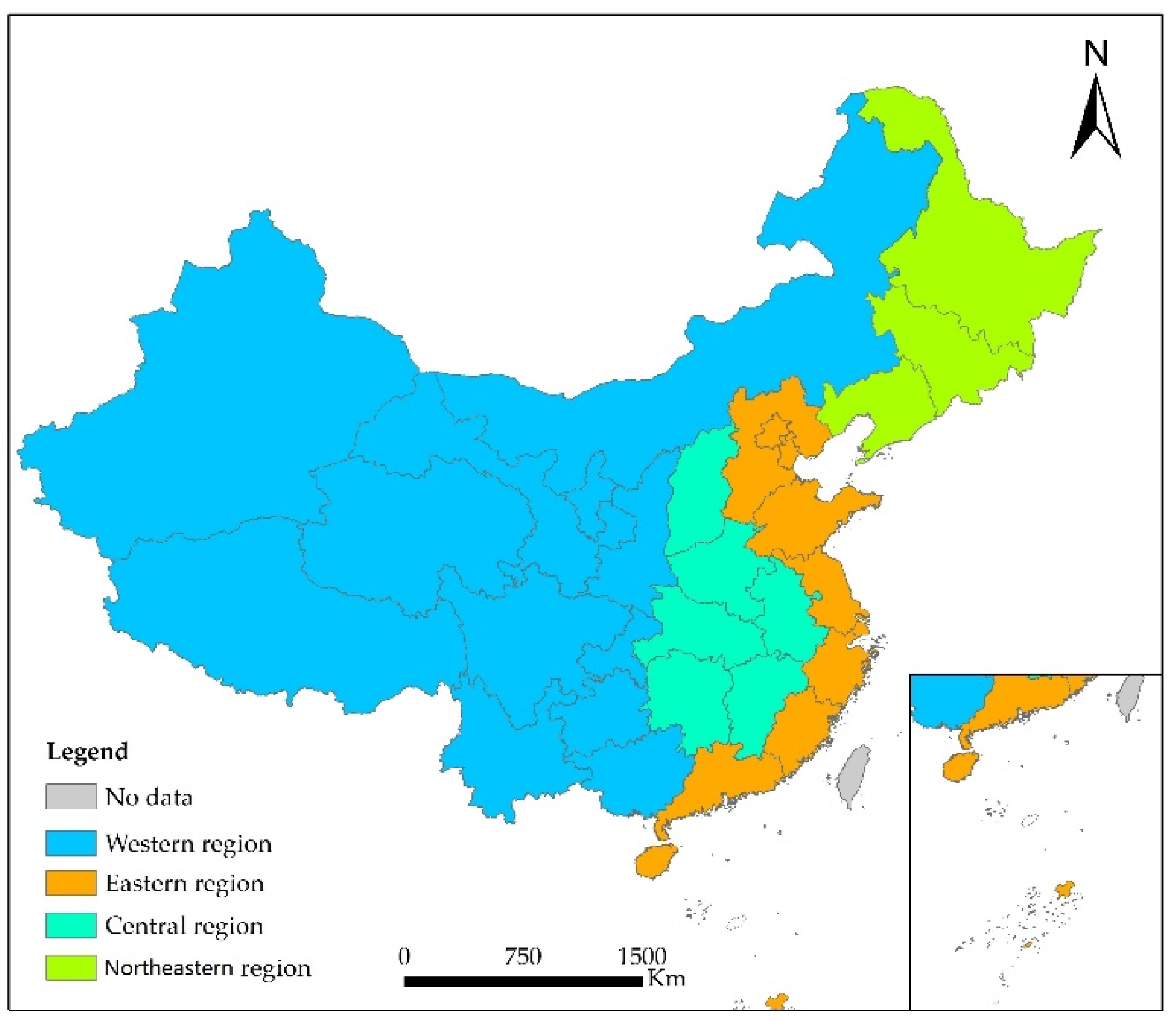
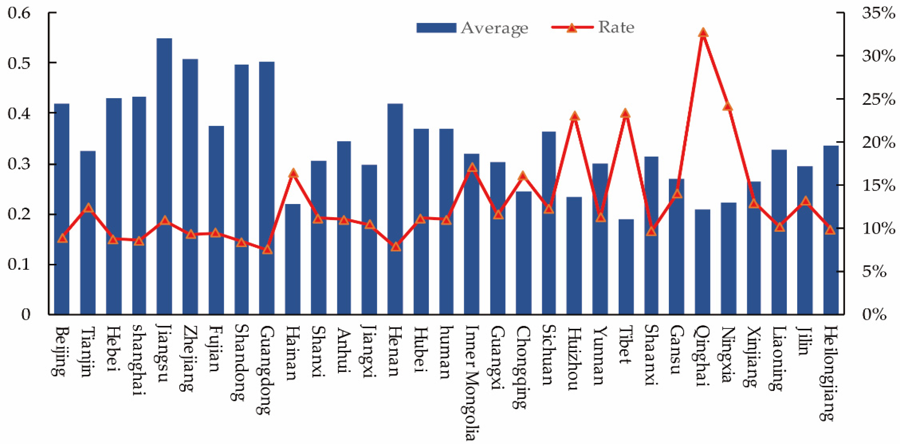
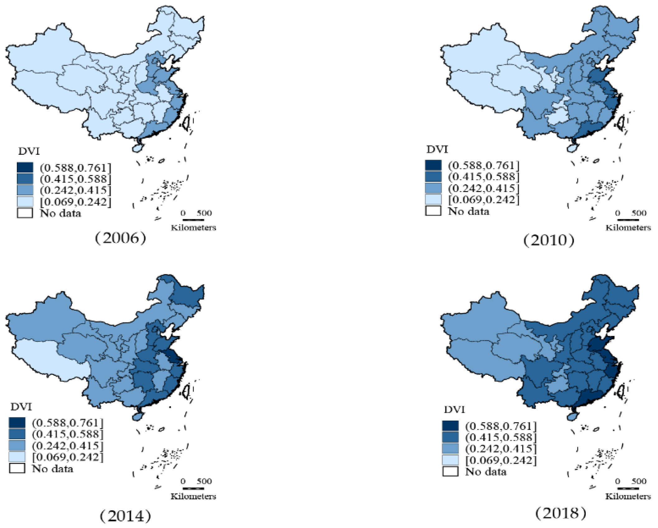
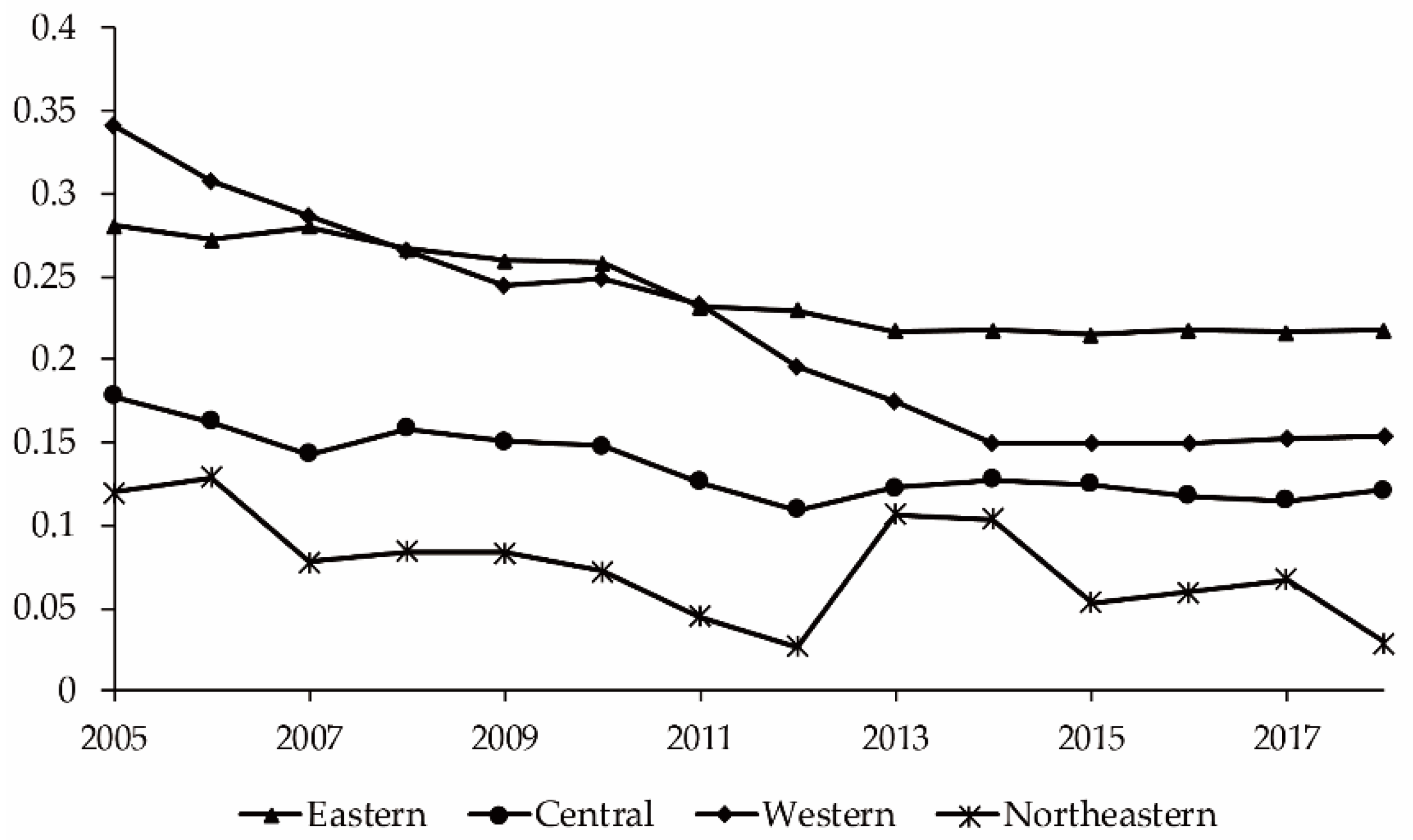
3.1. General Description of DVI in China and Four Major Regions

Based on the comprehensive evaluation model of the entropy method, we calculated the DVI of 31 provinces from 2005 to 2018 (Figure 2). The DVI of China shows a steady and continuous upward trend, with the comprehensive index rising from 0.196 in 2005 to 0.487 in 2018, with an average annual growth rate of 10.42%. The DVI in eastern China was significantly higher than in other regions, and the average comprehensive index was 0.426; the average value of the DVI was 0.351 and 0.320, respectively, in the central region and northeastern region, and the lowest DVI was the western region, with the average value of 0.269. There are significant differences in the growth rates of DVI among the four regions. The western region had the fastest growth rate with an average annual growth rate of 15.44%, followed by the northeastern region and the central region with an average annual growth rate of 10.95% and 10.33%. In contrast, the eastern region had the slowest growth rate, with an average annual growth rate of 9.50%.
Figure 3 is the spatial and temporal trend of DVI development in 31 provinces of mainland China in the past 2005–2018 years, which was drawn up by ArcGIS software. Due to the space limitation, it only lists the trend of DVI in the years 2006, 2010, 2014, and 2018. It can be seen from Figure 3 that the DVI in China has three characteristics in terms of space-time evolution: the level of China’s digital village development shows a relatively evident growth trend, the number of provinces with digital village development levels below 0.415 decreased from 22 to 8 provinces from 2006 to 2018, and the number of provinces above 0.588 increased by five provinces. The level of DVI in China is decreasing from the eastern to the western region. The provinces and cities with a higher level of DVI are mainly in the eastern region, such as Shandong, Jiangsu, Zhejiang, and Guangdong provinces; the provinces with low levels are primarily distributed in the western region, such as Xinjiang, Tibet, Qinghai, and Gansu provinces, and the level of DVI has been ranked lower. Thirdly, the level of DVI in China shows a significant trend of high-efficiency provinces from scattered distribution to eastern coastal agglomeration, and the DVI is relatively high mainly due to their superior geographical location, open market environment, and special transportation and logistics system.

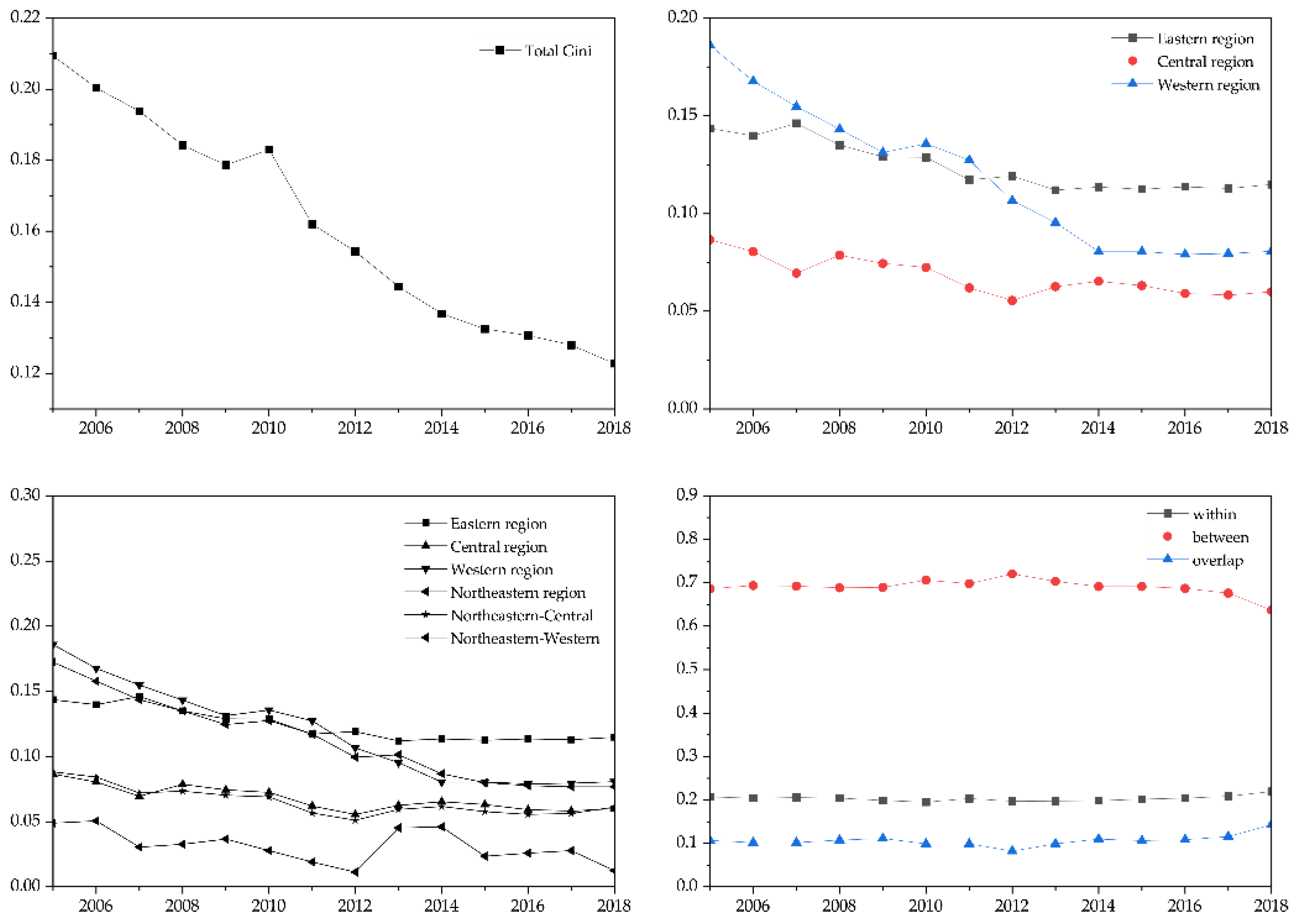
3.2. Regional Difference Decomposition of DVI

Using the Gini coefficient and decomposition method, this paper measured the overall Gini coefficient, inner-regional Gini coefficient, inter-regional Gini coefficient, and contribution rate of national and four regional DVI from 2005 to 2018. Figure 4 depicts the changing trend of the Gini coefficient of DVI in the nation during the sample period. The Gini coefficient of DVI in China decreased from 0.209 to 0.123, with an average annual decrease of 41.15%. This result showed that the spatial differentiation of digital rural development in China is on the decline.
Figure 4 depicts the changing trend of the Gini coefficient of DVI at the four regions during the sample period. The inner-regional difference degree of the eastern and western regions was the largest (the average Gini coefficient of the eastern and western regions was 0.124 and 0.118, respectively, during the sample period), while the inner-regional difference degree was small in the central and northeastern regions (the average Gini coefficients in the central and northeastern regions were 0.068 and 0.031, respectively, during the sample period). The Gini coefficient in the eastern, central, and western regions showed an obvious downward trend from the changing trend. In contrast, the Gini coefficient in the eastern region first decreased, then increased, and then decreased.
Figure 4 depicts the changing trend of the inter-regional difference of DVI in China during the sample period. The average Gini coefficient between the eastern and western regions during the whole investigation period was 0.188, with the largest inter-regional difference among all regions. From the changing trend, the inter-regional differences between most regions showed a narrowing trend, among which the decline range between the western and northeast regions was the largest, with a decrease rate of 55.50%. In contrast, the inter-regional difference between the eastern and northeastern regions decreased the smallest by 23.63%.
Figure 4 depicts the changing trend of the contribution rate of each decomposition term of the Gini coefficient to the overall Gini coefficient during the sample period. The contribution rate of the inter-regional difference to the overall difference was the largest and showed a trend of rising first and then decreasing. Secondly, the inner-regional difference was more minor, and the contribution rate of trans variation intensity to the overall spatial difference was the smallest.

3.3. Convergence Analysis of DVI

3.3.1. σ -Convergence Analysis of DVI in China

According to the σ -convergence test method, the variation of convergence coefficient in China and four regions is shown in Figure 5. From the national level, the σ -convergence coefficient of DVI from 2005 to 2018 showed a declining trend, which indicates that DVI in China has evident σ -convergence. From the regional level, the eastern, central, and western regions showed a downward trend, indicating a convergence of DVI in the areas mentioned above. The σ -convergence coefficient of the northeastern region showed a downward trend of fluctuation. After reaching the minimum value (0.027) in 2012, it increased sharply (reached 0.106) in 2013 and fluctuated again. The DVI of the northeastern region had σ -convergence before 2012, and continues to be divergent, which indicates periodic σ -convergence in the northeast region.

3.3.2. β -Convergence analysis of DVI in China

Spatial Correlation Test

To analyze the spatial correlation and spatial heterogeneity of DVI in different regions of China, Geoda software was used to measure the spatial Moran’s I index of DVI in 31 provinces of China from 2005 to 2018 and draw the local Moran scatter diagram, as shown in Table 2 and Figure 6. According to the calculation results in Table 2, the overall Moran’s I index of China’s DVI was positive during the survey period, the index values ranged from 0.291 to 0.374, and the p-values were all less than 0.01, which all passed the 1% significance test. It shows that the spatial distribution of DVI in China is not disorderly, but there is a significant positive spatial correlation.
In this regard, this paper used Moran scatter chart and the local Moran’s I index to draw the LISA agglomeration map of DVI of 31 provinces in China in 2006, 2010, 2014, and 2018 (Figure 6). Figure 6 shows that the number of provinces with positive spatial correlation (HH cluster and LL cluster) was 7, 11, 10, and 6 in 2006, 2010, 2014, and 2018, respectively. The increase and decrease in the numbers show that HH and LL clusters in digital villages first increased and then decreased, while LH and HL clusters remained unchanged. From the time change of the local agglomeration characteristics of DVI in China’s provinces, the HH cluster area mainly concentrated in coastal areas, showing a specific diffusion effect, while the LL cluster showed a downward trend. The HH cluster in coastal regions and LL cluster in western regions dominated the global autocorrelation of DVI in China.

Absolute β -Convergence Analysis

The absolute β -convergence shows that under the same other conditions, the regions will eventually reach the same steady-state level as time goes on. The spatial autocorrelation model (SAR) or spatial error model (SEM) can be used to analyze the absolute convergence, and the applicability of the model is observed by the Lagrange multiplier test (LM) [54,55]. For the whole region, LM test results are shown in Table 3. The results of the Lagrange multiplier test (LM) show that LM lag statistics and LM error statistics were significant at 1% level, robust LM lag statistics were not significant, and LM error statistics were significant at 1% level, which indicates that the spatial error model (SEM) is more suitable for the absolute β -convergence analysis. Absolute β -convergence results of DVI are shown in Table 4.
It can be seen from Table 4 that the coefficients of national, eastern, and northeastern regions were all negative in terms of the spatial autoregressive model (SAR) and spatial error model (SEM), and all passed the significance test at the level of 1%, indicating that there was absolute β -convergence in DVI in the eastern and northeastern regions. The convergence coefficient of the central and western regions was negative but not significant, indicating no evident absolute β -convergence trend in the DVI in the central and western regions. The results of the SEM model show that the convergence rate of DVI in the national, eastern, central, western, and northeastern regions was 0.26%, 0.34%, 0.05%, 0.11%, and 0.40%. The convergence rate of the northeastern was the fastest, followed by the eastern and western regions, and the central region was the slowest.

Conditional β -Convergence Analysis

The conditional β -convergence is that after considering the heterogeneity of each region, the DVI of each region will converge to its steady-state level over time, rather than the same steady-state level. Therefore, in the specific study of the convergence of DVI, this paper selected the control variables such as rural population density (DEN), industrial structure (STR), urbanization rate (URB), economic development level (ECO), openness (OPE), government influence (GOV), and other control variables. Rural population density (DEN), a measure of population density, is expressed by the number of rural populations per unit area of land. Industrial structure (STR) is defined by the ratio of the tertiary industry to GDP, which measures the industrial development. The level of urbanization (URB) is expressed by the proportion of the urban population to the total population. The level of economic development (ECO) is expressed in per capita GDP. The degree of opening to the outside world (OPE) is defined by the total import and export ratio to the GDP to measure the degree of regional openness. Government influence (GOV) is expressed by the proportion of the government’s agricultural budget expenditure (agricultural, forestry, and water finance expenditure) in GDP.
As with the absolute β -convergence, before the conditional β -convergence analysis, selecting the appropriate spatial econometric model is necessary. For the whole country, the LM test results are shown in Table 5. The Lagrange multiplier test (LM) results show that LM error statistics and LM lag statistics were significant at the level of 1%, robust LM error statistics were significant at the level of 1%. Robust LM lag statistics were significant at the level of 5%. The LM error statistic was more significant. Hence, the SEM model is the main model in this paper to analyze the factors that influence the conditional spatial convergence of DVI. The β -convergence results of the digital rural development index condition are shown in Table 6.
As shown in Table 6, after introducing relevant control variables, the coefficients of the national, eastern, central, western, and northeastern regions were all negative. They passed the significance test, indicating significant conditional β -convergence for DVI in China and the four major regions. The LogL and conditional β -convergence models in China and four regions were improved, showing that conditional β -convergence is more explanatory than absolute β -convergence.
From the national perspective, the coefficient of the spatial error model (SEM) was −0.2529, and the convergence rate was 2.083%, which is 1.83 percentage points higher than that of absolute β -convergence. The three control variables of DEN, STR, and ECO all passed the significance test. The coefficients were 0.0252, 0.0169, and 0.0330, respectively, which indicated that rural population density, industrial structure, and economic development level had significant positive effects on the convergence of DVI.
From the regional point of view, the coefficients of eastern, central, western, and northeastern regions were all negative in terms of the spatial autoregressive model (SAR) or spatial error model (SEM). Through the significance test, it shows that the four regional DVI had conditional β -convergence. The ECO of the eastern region passed the significance test. The DEN, URB, ECO, OPE, and GOV in the central region passed the significance test. The DEN, URB, and ECO in the western region passed the significance test. The DEN, STR, URB, ECO, and OPE of northeast China passed the significance test. It shows that the driving factors and convergence of digital village development in different regions are different due to economic and social development heterogeneity. Therefore, it is necessary to formulate digital village development policy-making and planning should be treated differently.

4. Discussion

Based on the panel data of China’s provinces from 2005 to 2018, we used the entropy weight method to calculate China’s digital rural development index. On this basis, we used the spatial autoregressive model (SAR) and spatial error model (SEM) to analyze the spatial convergence of DVI. We found that: DVI shows an upward trend throughout the study period, mainly from the local government’s policy support for rural development and digital Internet technologies in China. China is the world’s most populous country and once faced severe poverty in rural development. After 40 years of exploration and rapid growth, China has entered a new phase of reform and opening-up [56]. China’s National People’s Congress has proposed implementing a rural revitalization strategy to broadly address the contradiction between people’s growing living needs and unbalanced development, promoting rapid rural development [57]. In addition, China has the most significant number of Internet users in the world, and the emergence of the Internet has dramatically changed rural lifestyles and communication behaviors and positively influenced the development of residential villages [58]. The Chinese government has also issued policy documents to encourage the Internet to enter the countryside and create new possibilities for rural economic development through Internet e-commerce [59]. Second, China’s digital village development index as a whole showed a decreasing trend from the eastern region to the western region throughout the study period, and the level of digital village development in the east was higher than that in the west. Some eastern provinces have high-high clustering, some western provinces have low-low clustering, and only a few provinces have high-low aggregation or low-high clustering. This finding is consistent with Huang et al. [60] and Song et al. [61] on Internet-related studies in China. This is mainly due to economic factors and differences in infrastructure. The eastern region has a higher economic level in general, followed by the central region, and the western region has the lowest economic level. The acceptance and application of Internet digital information technology are higher in areas with higher economic levels than in less economically developed areas, and the construction of Internet infrastructure in villages requires higher funding, and some villages in the western region have difficulty maintaining the cost of installing Internet infrastructure due to lower economic levels [62]. Another critical factor is population density. Eastern China has a high population density in the countryside and a high degree of crowd gathering. In contrast, the less economically developed central and western regions have a small population density in the country and a lack of people utilizing the Internet and digital technology [63].
We also found that all four regions showed σ -convergence over the sample period, and the Dagum Gini coefficient decomposition also indicated that the differences between regions are gradually decreasing, which indicated that the differences in China’s digital countryside index within the four regions gradually narrow. With the inter-regional factors such as transportation channels, information networks, energy and electricity, and technology flow channels in central and western China [64], the digital capacity of each region’s villages can be promoted comprehensively, and the difference in the development level of digital villages between regions is gradually reduced. Of course, we analyzed the factors affecting digital rural development in China using an econometric model. According to the findings, there is absolute β -convergence in the national, eastern, and northeastern regions, and the conditional β -convergence results found that although there are differences in the factors affecting the level of digital rural development in the eastern, central, western, and northeastern regions, urbanization significantly affects the level of digital rural development in all four regions. In fact, according to the traditional economic theory of urban–rural dual structure and gradient economic theory, most scholars believe that most economic and social development occurs in urban areas with better resource endowment advantages. Furthermore, the development of urbanization will have a siphoning effect on the population and resources of villages [65,66,67], resulting in the gradual loss of rural resources and the deterioration of rural development [68]. However, with the continuous circulation of urban and rural factors in China, the interaction channel between rural and urban areas has been widened through state macro-control, market mechanism, and social dynamics [69], which can effectively increase the frequency and rate of urban–rural exchanges and jointly guarantee the multi-directional circulation of production factors. Moreover, this has become the fundamental driving force for rural development [70,71].

5. Conclusions and Policy Recommendations

This study found that the level of digital village development in China is uneven between regions, with considerable differences in development levels between provinces and regions. However, the level of digital village development among provinces shows an obvious aggregation effect, and the difference in the level of development among regions is gradually decreasing. Moreover, over time, the development level of the digital countryside between regions is converging toward their respective steady-state levels, and this steady-state level depends on each province’s own characteristics. This means that the steady-state level of the digital countryside in all provinces is different, so the digital countryside development gap between provinces will persist. Therefore, in the process of formulating the overall development policy of the digital countryside, it is necessary to formulate a policy and development plan that is consistent with the development of each region’s differentiated policies and development plans.
Based on the empirical research conclusions and relevant analysis, the specific policy recommendations include the following aspects: we must attach great importance to the spatial correlation and non-equilibrium characteristics of a country’s digital village development. Due to the significant positive spatial correlation and agglomeration effect of the development level of digital villages in China, the development level of digital villages in each province is affected by neighboring provinces. Therefore, it is necessary to strengthen exchanges and cooperation with adjacent regions and build a typical state through cross-regional cooperation and exchanges. A comprehensive, multi-domain regional digital village exchange and cooperation mechanism will be established, and the regional policy synergy effect and the demonstration and leading role of high-level digital village areas will be effectively brought into play. At the same time, attention should be paid to the radiating and driving function of the “growth pole” in the development of inter-provincial digital villages. Knowledge spillover, technology diffusion, and industrial linkage should promote the flow and sharing of digital village development elements, such as cooperative community to weaken and eliminate potential polarization. The government should focus on the LL provinces in Moran’s I scatter plot to prevent these provinces from falling into the path-dependence trap of being “locked” to a low level. For these provinces, it is necessary to take the lead in cultivating several cities with foundation and development potential and build them into the growth poles of the province’s digital villages. Development has a radiating and driving effect, which enhances the level of digital rural development in these provinces. Finally, due to differences in development foundations and resource endowments, the development of digital villages in various country regions is uneven, and the convergence situations in the country and the four major regions are also different. Therefore, government departments should formulate digital village development policies according to local conditions in light of their conditions. In addition to creating a good flow of elements in the central, western, and northeastern regions, it is also necessary to improve the total construction capacity of digital village development. Through a two-pronged approach, the synergistic effect of regional and inter-provincial digital villages should be realized, and efficiency and fairness should be considered, which is conducive to the development of digital villages.
Of course, although the current study confirms the potential contribution to the evaluation of China’s digital countryside, there are still certain limitations that are expected to be studied and addressed in the future. First, due to difficulties in data collection, especially the lack of data from Taiwan Province, Hong Kong, and Macau, this paper only covers data from 31 provinces and regions in mainland China, leading to incompleteness in the evaluation of the development level of the digital countryside in China as a whole. Secondly, only the factors affecting China’s digital countryside index are discussed econometrically, and the current study lacks an evaluation of a more extensive scope or a more comprehensive evaluation. Therefore, future work will expand the scope of the survey so that this research can be more generalizable. We also used the entropy weight method to measure the index weight of digital villages. However, this method is an objective weighting method that determines the weight of decision-making indicators according to the amount of information contained in each index value, so the evaluation results may be quite different from the facts. In the future, the subjective weighting method should be appropriately combined to determine the weight of evaluation indicators more scientifically.

Author Contributions

Conceptualization, X.L. and R.B.S.C.; methodology, X.L. and R.B.S.C.; software, R.B.S.C., X.L. and X.X.; validation, X.L., R.B.S.C. and X.X.; formal analysis, R.B.S.C. and X.L.; investigation, X.L. and R.B.S.C.; resources, X.L. and R.B.S.C.; data curation, R.B.S.C. and X.L.; writing—original draft preparation, R.B.S.C. and X.L.; writing—review and editing, X.L., R.B.S.C. and X.X.; visualization, R.B.S.C.; supervision, X.X.; project administration, X.X. and X.L.; funding acquisition, X.X. All authors have read and agreed to the published version of the manuscript.

Funding

The authors are grateful for the financial support by The National Social Science Fund of China (NOS. 21BJY187).

Institutional Review Board Statement

As the study does not involve any personal data and the respondent was well aware that they can opt-out anytime during the data collection phase, any written institutional review board statement is not required.

Informed Consent Statement

As the study does not involve any personal data and the respondent was well aware that they can opt-out anytime during the data collection phase, any written institutional review board statement is not required.

Data Availability Statement

The associated dataset of the study is available upon request to the corresponding author.

Conflicts of Interest

The authors declare no conflict of interest.

References

  1. Litan, R.E.; Rivlin, A.M. Projecting the Economic Impact of the Internet. Am. Econ. Rev. 2001, 91, 313–317. [Google Scholar] [CrossRef]
  2. Kim, D. A 2020 Perspective on “A Dynamic Model for the Evolution of the next Generation Internet—Implications for Network Policies”: Towards a Balanced Perspective on the Internet’s Role in the 5G and Industry 4.0 Era. Electron. Commer. Res. Appl. 2020, 41, 100966. [Google Scholar] [CrossRef]
  3. Maurseth, P.B. The Effect of the Internet on Economic Growth: Counter-Evidence from Cross-Country Panel Data. Econ. Lett. 2018, 172, 74–77. [Google Scholar] [CrossRef]
  4. Gabellone, F.; Lanorte, A.; Masini, N.; Lasaponara, R. From Remote Sensing to a Serious Game: Digital Reconstruction of an Abandoned Medieval Village in Southern Italy. J. Cult. Herit. 2017, 23, 63–70. [Google Scholar] [CrossRef]
  5. Xia, X.; Chen, Z.; Zhang, H.; Zhao, M. Agricultural High-Quality Development: Digital Empowerment and Implementation Path. Chin. Rural Econ. 2019, 420, 2–15. [Google Scholar]
  6. Bonati, L.; Polese, M.; D’Oro, S.; Basagni, S.; Melodia, T. Open, Programmable, and Virtualized 5G Networks: State-of-the-Art and the Road Ahead. Comput. Netw. 2020, 182, 107516. [Google Scholar] [CrossRef]
  7. Varghese, P. Exploring Other Concepts of Smart-Cities within the Urbanising Indian Context. Procedia Technol. 2016, 24, 1858–1867. [Google Scholar] [CrossRef] [Green Version]
  8. Lawson, P. Telecommunications Regulation: Creating Order & Opportunity in UK Digital Terrestrial Television Whitespace. Comput. Law Secur. Rev. 2014, 30, 375–391. [Google Scholar] [CrossRef]
  9. Ydersbond, I.M.; Auvinen, H.; Tuominen, A.; Fearnley, N.; Aarhaug, J. Nordic Experiences with Smart Mobility: Emerging Services and Regulatory Frameworks. Transp. Res. Procedia 2020, 49, 130–144. [Google Scholar] [CrossRef]
  10. Visvizi, A.; Lytras, M.D. Sustainable Smart Cities and Smart Villages Research: Rethinking Security, Safety, Well-Being, and Happiness. Sustainability 2019, 12, 215. [Google Scholar] [CrossRef] [Green Version]
  11. Visvizi, A.; Lytras, M.D. Rescaling and Refocusing Smart Cities Research: From Mega Cities to Smart Villages. JSTPM 2018, 9, 134–145. [Google Scholar] [CrossRef]
  12. Bielska, A.; Stańczuk-Gałwiaczek, M.; Sobolewska-Mikulska, K.; Mroczkowski, R. Implementation of the Smart Village Concept Based on Selected Spatial Patterns—A Case Study of Mazowieckie Voivodeship in Poland. Land Use Policy 2021, 104, 105366. [Google Scholar] [CrossRef]
  13. Berghel, H. Digital Village: Predatory Disintermediation. Commun. ACM 2000, 43, 23–29. [Google Scholar] [CrossRef]
  14. Tang, N.; Marshall, W.F. Centrosome Positioning in Vertebrate Development. J. Cell Sci. 2012, 125, 4951–4961. [Google Scholar] [CrossRef] [PubMed] [Green Version]
  15. Shen, Y.; Wu, J.; Li, D. Research on Micro Measurement Model of Digital Village Based on Entropy Weight Method. J. Libr. Inf. Sci. Agric. 2020, 34, 68–76. [Google Scholar]
  16. Zhang, H.; Du, K.; Jin, B. Research on the Evaluation of Digital Rural Development Readiness under the Strategy of Rural Revitalization. J. Univ. Financ. Econ. 2020, 33, 51–60. [Google Scholar] [CrossRef]
  17. Fang, Y. Construction and Analysis of Digital Village Evaluation Index System. Shanxi Agric. Econ. 2020, 275, 21–23. [Google Scholar] [CrossRef]
  18. Zhang, W.; Wang, M.Y. Spatial-Temporal Characteristics and Determinants of Land Urbanization Quality in China: Evidence from 285 Prefecture-Level Cities. Sustain. Cities Soc. 2018, 38, 70–79. [Google Scholar] [CrossRef]
  19. Cui, Y.; Khan, S.U.; Deng, Y.; Zhao, M. Spatiotemporal Heterogeneity, Convergence and Its Impact Factors: Perspective of Carbon Emission Intensity and Carbon Emission per Capita Considering Carbon Sink Effect. Environ. Impact Assess. Rev. 2022, 92, 106699. [Google Scholar] [CrossRef]
  20. Shen, F. The Endogenous Development Model of Digital Village: Practical Logic, Operation Mechanism and Optimization Strategy. E-Government 2021, 226, 57–67. [Google Scholar]
  21. Wang, Y.; Wang, H. The Impact of Digital Village on Rural Residents’ Online Shopping. China Bus. Mark. 2021, 35, 9–18. [Google Scholar]
  22. Ranade, P.; Londhe, S.; Mishra, A. Smart Villages through Information Technology—Need of Emerging India. IPASJ Int. J. Inf. Technol. 2015, 3, 1–6. [Google Scholar]
  23. Daniel, S.; Doran, M.A. GeoSmartCity: Geomatics Contribution to the Smart City. In Proceedings of the International Conference on Digital Government Research: From E-government to Smart Government, Quebec City, QC, Canada, 17–20 June 2013. [Google Scholar] [CrossRef] [Green Version]
  24. Guo, H.; Chen, X. Building a “Digital Village” to Promote Rural Revitalization. Hangzhou Wkly. 2018, 47, 10–11. [Google Scholar]
  25. Irwansyah. The Social Contractual Utilitarianism of a Digital Village in Rural Indonesia. Technol. Soc. 2020, 63, 101354. [Google Scholar] [CrossRef]
  26. Shang, L.; Heckelei, T.; Gerullis, M.K.; Börner, J.; Rasch, S. Adoption and Diffusion of Digital Farming Technologies—Integrating Farm-Level Evidence and System Interaction. Agric. Syst. 2021, 190, 103074. [Google Scholar] [CrossRef]
  27. Wu, H.-W.; Li, E.; Sun, Y.; Dong, B. Research on the Operation Safety Evaluation of Urban Rail Stations Based on the Improved TOPSIS Method and Entropy Weight Method. J. Rail Transp. Plan. Manag. 2021, 20, 100262. [Google Scholar] [CrossRef]
  28. Tian, R.; Shao, Q.; Wu, F. Four-Dimensional Evaluation and Forecasting of Marine Carrying Capacity in China: Empirical Analysis Based on the Entropy Method and Grey Verhulst Model. Mar. Pollut. Bull. 2020, 160, 111675. [Google Scholar] [CrossRef]
  29. Li, Y.; Zhang, Q.; Wang, L.; Liang, L. Regional Environmental Efficiency in China: An Empirical Analysis Based on Entropy Weight Method and Non-Parametric Models. J. Clean. Prod. 2020, 276, 124147. [Google Scholar] [CrossRef]
  30. Zhao, J.; Ji, G.; Tian, Y.; Chen, Y.; Wang, Z. Environmental Vulnerability Assessment for Mainland China Based on Entropy Method. Ecol. Indic. 2018, 91, 410–422. [Google Scholar] [CrossRef]
  31. Dagum, C. A New Approach to the Decomposition of the Gini Income Inequality Ratio. Empir. Econ. 1997, 22, 515–531. [Google Scholar] [CrossRef]
  32. Thomson, E.M.; Bradley, B.A.; Lee, R.L.; Wotherspoon, L.M.; Wood, C.M.; Cox, B.R. Generalised Parametric Functions and Spatial Correlations for Seismic Velocities in the Canterbury, New Zealand Region from Surface-Wave-Based Site Characterisation. Soil Dyn. Earthq. Eng. 2020, 128, 105834. [Google Scholar] [CrossRef]
  33. Nguyen, T.T.; Vu, T.D. Identification of Multivariate Geochemical Anomalies Using Spatial Autocorrelation Analysis and Robust Statistics. Ore Geol. Rev. 2019, 111, 102985. [Google Scholar] [CrossRef]
  34. Jha, R.K.; Gundimeda, H.; Andugula, P. Assessing the Social Vulnerability to Floods in India: An Application of Superefficiency Data Envelopment Analysis and Spatial Autocorrelation to Analyze Bihar Floods. In Economic Effects of Natural Disasters; Elsevier: Amsterdam, The Netherlands, 2021; pp. 559–581. ISBN 978-0-12-817465-4. [Google Scholar]
  35. Melecky, L. Spatial Autocorrelation Method for Local Analysis of The EU. Procedia Econ. Financ. 2015, 23, 1102–1109. [Google Scholar] [CrossRef] [Green Version]
  36. Ren, H.; Shang, Y.; Zhang, S. Measuring the Spatiotemporal Variations of Vegetation Net Primary Productivity in Inner Mongolia Using Spatial Autocorrelation. Ecol. Indic. 2020, 112, 106108. [Google Scholar] [CrossRef]
  37. Hou, Y.; Zhang, K.; Zhu, Y.; Liu, W. Spatial and Temporal Differentiation and Influencing Factors of Environmental Governance Performance in the Yangtze River Delta, China. Sci. Total Environ. 2021, 801, 149699. [Google Scholar] [CrossRef]
  38. Tepanosyan, G.; Sahakyan, L.; Zhang, C.; Saghatelyan, A. The Application of Local Moran’s I to Identify Spatial Clusters and Hot Spots of Pb, Mo and Ti in Urban Soils of Yerevan. Appl. Geochem. 2019, 104, 116–123. [Google Scholar] [CrossRef]
  39. Das Majumdar, D.; Biswas, A. Quantifying Land Surface Temperature Change from LISA Clusters: An Alternative Approach to Identifying Urban Land Use Transformation. Landsc. Urban Plan. 2016, 153, 51–65. [Google Scholar] [CrossRef]
  40. Kuznetsov, A.; Sadovskaya, V. Spatial Variation and Hotspot Detection of COVID-19 Cases in Kazakhstan, 2020. Spat. Spatio-Temporal Epidemiol. 2021, 39, 100430. [Google Scholar] [CrossRef]
  41. Banerjee, A.; Singh, A.K.; Chaurasia, H. An Exploratory Spatial Analysis of Low Birth Weight and Its Determinants in India. Clin. Epidemiol. Glob. Health 2020, 8, 702–711. [Google Scholar] [CrossRef] [Green Version]
  42. Seya, H.; Tsutsumi, M.; Yamagata, Y. Income Convergence in Japan: A Bayesian Spatial Durbin Model Approach. Econ. Model. 2012, 29, 60–71. [Google Scholar] [CrossRef]
  43. He, S.; Jiang, L. Identifying Convergence in Nitrogen Oxides Emissions from Motor Vehicles in China: A Spatial Panel Data Approach. J. Clean. Prod. 2021, 316, 128177. [Google Scholar] [CrossRef]
  44. Baumont, C.; Ertur, C.; Le Gallo, J. Spatial Convergence Clubs and the European Regional Growth Process,1980–1995. In European Regional Growth; Fingleton, B., Ed.; Advances in Spatial Science; Springer: Berlin/Heidelberg, Germany, 2003; pp. 131–158. ISBN 978-3-642-05571-3. [Google Scholar]
  45. Boots, B.; Haining, R. Spatial Data Analysis in the Social and Environmental Sciences. Trans. Inst. Br. Geogr. 1993, 18, 287. [Google Scholar] [CrossRef]
  46. Cui, Y.; Wang, L.; Jiang, L.; Liu, M.; Wang, J.; Shi, K.; Duan, X. Dynamic Spatial Analysis of NO2 Pollution over China: Satellite Observations and Spatial Convergence Models. Atmos. Pollut. Res. 2021, 12, 89–99. [Google Scholar] [CrossRef]
  47. Jiang, L.; He, S.; Zhou, H. Spatio-Temporal Characteristics and Convergence Trends of PM2.5 Pollution: A Case Study of Cities of Air Pollution Transmission Channel in Beijing-Tianjin-Hebei Region, China. J. Clean. Prod. 2020, 256, 120631. [Google Scholar] [CrossRef]
  48. Hao, Y.; Peng, H. On the Convergence in China’s Provincial per Capita Energy Consumption: New Evidence from a Spatial Econometric Analysis. Energy Econ. 2017, 68, 31–43. [Google Scholar] [CrossRef]
  49. Gong, Y.; Hu, J.; Boelhouwer, P.J. Spatial Interrelations of Chinese Housing Markets: Spatial Causality, Convergence and Diffusion. Reg. Sci. Urban Econ. 2016, 59, 103–117. [Google Scholar] [CrossRef]
  50. Mishra, V.; Smyth, R. Conditional Convergence in Australia’s Energy Consumption at the Sector Level. Energy Econ. 2017, 62, 396–403. [Google Scholar] [CrossRef]
  51. Akram, V.; Rath, B.N.; Sahoo, P.K. Stochastic Conditional Convergence in per Capita Energy Consumption in India. Econ. Anal. Policy 2020, 65, 224–240. [Google Scholar] [CrossRef]
  52. Gotway, C.A.; Haining, R. Spatial Data Analysis in the Social and Environmental Sciences. Technometrics 1992, 34, 499. [Google Scholar] [CrossRef]
  53. Kassouri, Y.; Okunlola, O.A. Analysis of Spatio-Temporal Drivers and Convergence Characteristics of Urban Development in Africa. Land Use Policy 2021, 112, 105868. [Google Scholar] [CrossRef]
  54. Bartesaghi-Koc, C.; Osmond, P.; Peters, A. Innovative Use of Spatial Regression Models to Predict the Effects of Green Infrastructure on Land Surface Temperatures. Energy Build. 2022, 254, 111564. [Google Scholar] [CrossRef]
  55. Espoir, D.K.; Sunge, R. CO2 Emissions and Economic Development in Africa: Evidence from a Dynamic Spatial Panel Model. J. Environ. Manag. 2021, 300, 113617. [Google Scholar] [CrossRef] [PubMed]
  56. Guo, Y.; Liu, Y. Poverty Alleviation through Land Assetization and Its Implications for Rural Revitalization in China. Land Use Policy 2021, 105, 105418. [Google Scholar] [CrossRef]
  57. Yin, X.; Chen, J.; Li, J. Rural Innovation System: Revitalize the Countryside for a Sustainable Development. J. Rural Stud. 2019; in press. [Google Scholar] [CrossRef]
  58. Wu, H.; Ba, N.; Ren, S.; Xu, L.; Chai, J.; Irfan, M.; Hao, Y.; Lu, Z.-N. The Impact of Internet Development on the Health of Chinese Residents: Transmission Mechanisms and Empirical Tests. Socio-Econ. Plan. Sci. 2021, 101178. [Google Scholar] [CrossRef]
  59. Zhu, W.; Shang, F. Rural Smart Tourism under the Background of Internet Plus. Ecol. Inform. 2021, 65, 101424. [Google Scholar] [CrossRef]
  60. Huang, J.; Zhang, W.; Ruan, W. Spatial Spillover and Impact Factors of the Internet Finance Development in China. Phys. A Stat. Mech. Its Appl. 2019, 527, 121390. [Google Scholar] [CrossRef]
  61. Song, Z.; Wang, C.; Bergmann, L. China’s Prefectural Digital Divide: Spatial Analysis and Multivariate Determinants of ICT Diffusion. Int. J. Inf. Manag. 2020, 52, 102072. [Google Scholar] [CrossRef]
  62. Wang, D.; Zhou, T.; Lan, F.; Wang, M. ICT and Socio-Economic Development: Evidence from a Spatial Panel Data Analysis in China. Telecommun. Policy 2021, 45, 102173. [Google Scholar] [CrossRef]
  63. Liu, M.; Zhang, Q.; Gao, S.; Huang, J. The Spatial Aggregation of Rural E-Commerce in China: An Empirical Investigation into Taobao Villages. J. Rural Stud. 2020, 80, 403–417. [Google Scholar] [CrossRef]
  64. Wu, H.; Hao, Y.; Ren, S.; Yang, X.; Xie, G. Does Internet Development Improve Green Total Factor Energy Efficiency? Evidence from China. Energy Policy 2021, 153, 112247. [Google Scholar] [CrossRef]
  65. Li, H.; Yuan, Y.; Zhang, X.; Li, Z.; Wang, Y.; Hu, X. Evolution and Transformation Mechanism of the Spatial Structure of Rural Settlements from the Perspective of Long-Term Economic and Social Change: A Case Study of the Sunan Region, China. J. Rural Stud. 2019, S0743016718301487. [Google Scholar] [CrossRef]
  66. Cheng, L. China’s Rural Transformation under the Link Policy: A Case Study from Ezhou. Land Use Policy 2021, 103, 105319. [Google Scholar] [CrossRef]
  67. Xu, W.; Pan, Z.; Wang, G. Market Transition, Labor Market Dynamics and Reconfiguration of Earning Determinants Structure in Urban China. Cities 2018, 79, 113–123. [Google Scholar] [CrossRef]
  68. Liu, Y.; Zhou, Y.; Li, Y. Rural Regional System and Rural Revitalization Strategy in China. Acta Geogr. Sin. 2019, 74, 2511–2528. [Google Scholar] [CrossRef]
  69. Wong, S.W.; Dai, Y.; Tang, B.; Liu, J. A New Model of Village Urbanization? Coordinative Governance of State-Village Relations in Guangzhou City, China. Land Use Policy 2021, 109, 105500. [Google Scholar] [CrossRef]
  70. Zhu, J.; Zhu, M.; Xiao, Y. Urbanization for Rural Development: Spatial Paradigm Shifts toward Inclusive Urban-Rural Integrated Development in China. J. Rural Stud. 2019, 71, 94–103. [Google Scholar] [CrossRef]
  71. Chen, K.; Long, H.; Liao, L.; Tu, S.; Li, T. Land Use Transitions and Urban-Rural Integrated Development: Theoretical Framework and China’s Evidence. Land Use Policy 2020, 92, 104465. [Google Scholar] [CrossRef]
Figure 1. Data source for four regions in China.
Agriculture 12 00164 g001
Figure 2. Average DVI and growth rates of 31 provinces from 2005 to 2018.
Agriculture 12 00164 g002
Figure 3. Spatial and temporal evolution trend of DVI in China.
Agriculture 12 00164 g003
Figure 4. Gini coefficient variation and differential contribution rate of DVI in China.
Agriculture 12 00164 g004
Figure 5. The change of σ -convergence coefficient of DVI in China.
Agriculture 12 00164 g005
Figure 6. Lisa cluster map of DVI in China.
Agriculture 12 00164 g006
Table 1. The evaluation index system of DVI.
Primary IndicatorsSecondary IndicatorsUnitWeight (%)
Main development ability
(31.9591%)
Per capita disposable income of rural residentsYuan/person9.7124
Consumption level of rural residentsYuan/person6.9659
Average education level of rural residentsYear7.5285
Per capita expenditure on transportation and communication of rural residentsYuan/person7.7523
Infrastructure construction (40.9690%)Length of long-distance optical cable lineKm6.1673
Length of rural delivery route of long-distance optical cable line (one way)Km10.0915
Proportion of administrative villages with Internet broadband services%2.5326
Proportion of postal administrative villages%2.8889
Total power of agricultural machineryTen thousand kw8.4360
Rural power consumptionTen thousand kw/h7.5282
Average weekly delivery times in rural areasTimes3.3245
Information environment (27.0719%)Internet penetration rate%8.0714
Number of color TV sets per 100 rural householdsSet2.9976
Mobile phone ownership per 100 rural householdsDepartment7.0624
Computer ownership per 100 rural householdsSet8.9405
Notes: The weights of each dimension are in parentheses.
Table 2. Global Moran’s Index of DVI in China from 2005 to 2018.
Year20052006200720082009201020112012201320142015201620172018
Moran’s I0.3060.3130.3150.3030.3180.3740.3360.3600.3520.3500.3260.3090.2910.253
Z-value2.8392.9002.9182.8122.9313.3973.0943.3083.2403.2213.0312.9042.7562.421
p-value0.0020.0020.0020.0020.0020.0000.0010.0000.0010.0010.0010.0020.0030.008
Table 3. Results of Lagrange multiplier (LM) test.
Test MethodStatisticp-ValueTest MethodStatisticp-Value
Lagrange multiplier (error)69.7810.000Robust Lagrange multiplier (error)28.8160.000
Lagrange multiplier (lag)42.2070.000Robust Lagrange multiplier (lag)1.2410.265
Table 4. Results of absolute β -convergence regression.
ModelSARSEM
RegionsNationalEasternCentralWesternNortheasternNationalEasternCentralWesternNortheastern
β −0.0166 ***
(0.0055)
−0.0347 ***
(0.0076)
−0.0046
(0.0139)
−0.0039
(0.0064)
−0.0488 ***
(0.0136)
−0.0351 ***
(0.0086)
−0.0466 ***
(0.0091)
−0.0063
(0.0164)
−0.0157
(0.0119)
−0.0542 ***
(0.0143)
ρ 0.3911 ***
(0.0431)
0.2212 ***
(0.0447)
0.1171 ***
(0.0362)
0.4742 ***
(0.0421)
0.0624 *
(0.0353)
λ 0.4161 ***
(0.0418)
0.2378 ***
(0.0423)
0.1209 ***
(0.0428)
0.4848 ***
(0.0417)
0.0872 ***
(0.0230)
LogL1343.4135433.8977269.2690530.4190117.40421345.4145434.3711269.2926530.7026117.4802
R 2 0.00330.09830.00080.00020.07010.02230.10320.00110.00010.0728
Notes: * and *** are significant at 10% and 1% levels, respectively, and the values in brackets are standard errors.
Table 5. Results of Lagrange multiplier (LM) test.
Test MethodStatisticp-ValueTest MethodStatisticp-Value
Lagrange multiplier (error)51.5790.000Robust Lagrange multiplier (error)8.7070.003
Lagrange multiplier (lag)48.2590.000Robust Lagrange multiplier (lag)5.3870.020
Table 6. Results of conditional β -convergence regression.
ModelSARSEM
RegionsNationalEasternCentralWesternNortheasternNationalEasternCentralWesternNortheastern
β −0.2332 ***
(0.0419)
−0.2460 ***
(0.0773)
−0.4911 ***
(0.0802)
−0.2145 ***
(0.0623)
−0.6787 ***
(0.1696)
−0.2529 ***
(0.0438)
−0.2450 ***
(0.0749)
−0.4714 ***
(0.0741)
−0.2098 ***
(0.0582)
−0.6944 ***
(0.1709)
ρ 0.3238 ***
(0.0462)
0.1873 ***
(0.0425)
0.1108 ***
(0.0409)
0.4274 ***
(0.0486)
−0.0524
(0.0966)
λ 0.3440 ***
(0.0451)
0.1829 ***
(0.0442)
0.1461 **
(0.0695)
0.4413 ***
(0.0467)
−0.1103 *
(0.0668)
Ln DEN0.0288 **
(0.0115)
0.0107
(0.0294)
0.1102 ***
(0.0321)
0.0499 **
(0.0227)
−0.2178 **
(0.0917)
0.0252 **
(0.0100)
0.0048
(0.0300)
0.1230 ***
(0.0278)
0.0517 **
(0.0245)
−0.2321 **
(0.1019)
Ln STR0.0207 **
(0.0083)
0.0258
(0.0214)
0.0146
(0.0101)
0.0146
(0.0164)
0.1143 ***
(0.0379)
0.0169 **
(0.0081)
0.0231
(0.0214)
0.0105
(0.0122)
0.0114
(0.0141)
0.1222 ***
(0.0428)
Ln URB0.0118
(0.0108)
−0.0099
(0.0403)
0.1656 ***
(0.0362)
0.0651 ***
(0.00232)
−0.3658 **
(0.1616)
0.0140
(0.0121)
−0.0222
(0.0435)
0.1696 ***
(0.0416)
0.0556 ***
(0.0217)
−0.4087 **
(0.1931)
Ln ECO0.0321 ***
(0.0067)
0.0368***
(0.0132)
0.0538 ***
(0.0101)
0.0162 **
(0.0075)
0.0959 ***
(0.0276)
0.0330 ***
(0.0070)
0.0369 ***
(0.0136)
0.0538 ***
(0.0094)
0.0176 **
(0.0086)
0.1012 ***
(0.0315)
Ln OPE−0.0025
(0.0027)
0.0006
(0.0072)
−0.0222 **
(0.0095)
0.0014
(0.0030)
0.0481 ***
(0.0169)
−0.0035
(0.0027)
−0.0014
(0.0083)
−0.0223 **
(0.0098)
0.0016
(0.0025)
0.0487 ***
(0.0136)
Ln GOV−0.0036 *
(0.0021)
−0.0038
(0.0049)
−0.0252 ***
(0.0029)
−0.0001
(0.0030)
−0.0068
(0.0068)
−0.0022
(0.0025)
−0.0031
(0.0055)
−0.0267 ***
(0.0044)
0.0022
(0.0036)
−0.0097
(0.0093)
LogL1380.1760443.7616286.5129542.8184129.29421380.0814443.1522286.6016541.2971129.4549
R 2 0.21410.24660.35680.21460.49400.20830.23520.35410.16430.4958
Notes: *, **, and *** are significant at 10%, 5%, and 1% levels, respectively, and the values in brackets are standard errors.
Publisher’s Note: MDPI stays neutral with regard to jurisdictional claims in published maps and institutional affiliations.

