
Prediction of Blueberry (Vaccinium corymbosum L.) Yield Based on Artificial Intelligence Methods

 ,
,  ,
,  ,
,  ,
,  and
and
Abstract
1. Introduction
2. Materials and Methods
2.1. Dataset Description
2.1.1. Agronomical Data
2.1.2. BBCH-Scale
- (1)
- BBCH 0–60 (from dormancy to the beginning of flowering)
- (2)
- BBCH 61–70 (from the beginning of flowering to the end of flowering
- (3)
- BBCH > 70 (from the beginning of fruit growth to harvest)
2.1.3. Numerical Features
- (1)
- Air temperature (avg.) [°C]
- (2)
- Air temperature (max.) [°C]
- (3)
- Air temperature (min.) [°C]
- (4)
- Rainfall [mm]
- (5)
- Air relative humidity (avg.) [%]
- (6)
- Air relative humidity (max.) [%]
- (7)
- Air relative humidity (min.) [%]
- (8)
- Dew point temperature (avg.) [°C]
- (9)
- Dew point temperature (max.) [°C]
- (10)
- Dew point temperature (min.) [°C]
- (1)
- Irrigation [kg]
- (2)
- Fertigation [l]
- (1)
- pH
- (2)
- S-SO—sulfur [mg/L]
- (3)
- P—phosphorus [mg/L]
- (4)
- K—potassium [mg/L]
- (5)
- C—calcium [mg/L]
- (6)
- Mg—magnesium [mg/L]
- (7)
- Fe—iron [mg/L]
- (8)
- Zn—zinc [mg/L]
- (9)
- Mn—manganese [mg/L]
- (10)
- Cu—copper [mg/L]
- (11)
- B—boron [mg/L]
- (12)
- Cl—chlorine [mg/L]
- (13)
- Na—sodium [mg/L]
- (14)
- N-NO—nitrogen [mg/L]
2.1.4. BBCH Soil and Climate Features
- (1)
- Insolation (BBCH 0–60) [W/m]
- (2)
- Insolation (BBCH 61–70) [W/m]
- (3)
- Insolation (BBCH > 70) [W/m]
- (4)
- Rainfall (BBCH 0–60) [mm]
- (5)
- Rainfall (BBCH 61–70) [mm]
- (6)
- Rainfall (BBCH > 70) [mm]
- (7)
- Irrigation (BBCH 0–60) [mm]
- (8)
- Irrigation (BBCH 61–70) [mm]
- (9)
- Irrigation (BBCH > 70) [mm]
- (10)
- Daily air temperature (avg.) (BBCH 0–60) [°C]
- (11)
- Daily air temperature (avg.) (BBCH 61–70) [°C]
- (12)
- Daily air temperature (avg.) (BBCH > 70) [°C]
- (13)
- Daily soil temperature (avg.) (BBCH 0–60) [°C]
- (14)
- Daily soil temperature (avg.) (BBCH 61–70) [°C]
- (15)
- Daily soil temperature (avg.) (BBCH > 70) [°C]
- (16)
- Soil pH (avg.) (BBCH 0–60)
- (17)
- Soil pH (avg.) (BBCH 61–70)
- (18)
- Soil pH (avg.) (BBCH > 70)
- (19)
- Soil humidity (avg.) (BBCH 0–60) [%]
- (20)
- Soil humidity (avg.) (BBCH 61–70) [%]
- (21)
- Soil humidity (avg.) (BBCH > 70) [%]
- (22)
- Soil P—phosphorus (avg.) (BBCH 0–60) [mg/L]
- (23)
- Soil P—phosphorus (avg.) (BBCH 61–70) [mg/L]
- (24)
- Soil P—phosphorus (avg.) (BBCH > 70) [mg/L]
- (25)
- Soil Mg—magnesium (avg.) (BBCH 0–60) [mg/L]
- (26)
- Soil Mg—magnesium (avg.) (BBCH 61–70) [mg/L]
- (27)
- Soil Mg—magnesium (avg.) (BBCH > 70) [mg/L]
- (28)
- Soil K—potassium (avg.) (BBCH 0–60) [mg/L]
- (29)
- Soil K—potassium (avg.) (BBCH 61–70) [mg/L]
- (30)
- Soil K—potassium (avg.) (BBCH > 70) [mg/L]
2.1.5. Vegetation Features
- (1)
- EVI—Enhanced Vegetation Index
- (2)
- NDVI—Normalized Difference Vegetation Index
- (3)
- RDVI—Renormalized Difference Vegetation Index
- (4)
- SAVI—Soil-Adjusted Vegetation Index
- (1)
- EVI 40 days before harvest (max.)
- (2)
- EVI 40 days before harvest (avg.)
- (3)
- EVI 40 days before harvest (min.)
- (4)
- EVI 40 days before harvest (stddev.)
- (5)
- NDVI 40 days before harvest (max.)
- (6)
- NDVI 40 days before harvest (avg.)
- (7)
- NDVI 40 days before harvest (min.)
- (8)
- NDVI 40 days before harvest (stddev.)
- (9)
- RDVI 40 days before harvest (max.)
- (10)
- RDVI 40 days before harvest (avg.)
- (11)
- RDVI 40 days before harvest (min.)
- (12)
- RDVI 40 days before harvest (stddev.)
- (13)
- SAVI 40 days before harvest (max.)
- (14)
- SAVI 40 days before harvest (avg.)
- (15)
- SAVI 40 days before harvest (min.)
- (16)
- SAVI 40 days before harvest (stddev.)
2.1.6. Selyaninov Hydrothermal Coefficient
- (1)
- HTC (BBCH 0–60)
- (2)
- HTC (BBCH 61–70)
- (3)
- HTC (BBCH > 70)
2.1.7. GDD Features
- (1)
- GDD (BBCH 0–60)
- (2)
- GDD (BBCH 61–70)
- (3)
- GDD (BBCH > 70)
2.1.8. Aggregates Based on Mineral Fertilization and Fertigation
- (1)
- Fertilization (BBCH 0–60) [kg]
- (2)
- Fertilization (BBCH 61–70) [kg]
- (3)
- Fertilization (BBCH > 70) [kg]
- (4)
- Fertigation (BBCH 0–60) [l]
- (5)
- Fertigation (BBCH 61–70) [l]
- (6)
- Fertigation (BBCH > 70) [l]
- (7)
- K—potassium-Fertilization (annually) [kg]
- (8)
- N—nitrogen-Fertilization (annually) [kg]
- (9)
- P—phosphorus-Fertilization (annually) [kg]
2.1.9. Harmful Features
- (1)
- hailstorm percentage of damage [%]
- (2)
- hailstorm cut fruit [%]
2.1.10. Features Summary
2.2. Data Preprocessing Methods
2.2.1. Data Normalization
- (1)
- Crop/Harvest
- (2)
- Irrigation
- (3)
- Fertigation
- (1)
- hailstorm percentage of damage [%]
- (2)
- hailstorm cut fruit [%]
2.2.2. Finding and Replacing Missing Values
- (1)
- Imputation Using (Mean/Median) Values
- (2)
- Imputation Using (Most Frequent) or (Zero/Constant) Values
- (3)
- Stochastic Regression Imputation
- (4)
- Extrapolation and Interpolation
- (5)
- Imputation Using k-NN
- (6)
- Imputation Using XGBoost
- (7)
- Others
- (1)
- S-SO—sulfur
- (2)
- Cl—chlorine
- (3)
- Fertigation (BBCH 0–60)
- (4)
- Fertilization (BBCH 0–60)
- (5)
- Hailstorm percentage of damage
- (6)
- Hailstorm cut fruit
Extreme Gradient Boosting-XGBoost
| Algorithm 1: Algorithm of missing value imputation using XGBoost |
procedure FillMissingByXGBoost() ▹ do not touch real value of features return end procedure |
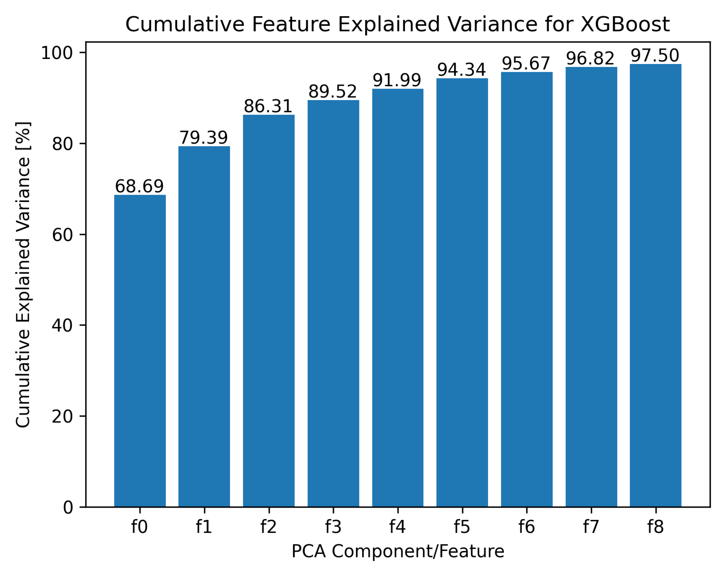
2.3. Feature Generation Using PCA (Principal Component Analysis) Method
2.4. Outlier Detection
2.4.1. Local Outlier Factor (LOF)
2.4.2. Unsupervised Outlier Detection Based on OneClassSVM
2.5. Feature Selection
2.5.1. Stepwise Regression
- (1)
- Fit the initial model.
- (2)
- If any features not in the model have a p-value less than the input tolerance (e.g., 0.05), add the one with the smallest p-value and repeat this step. For example, suppose the initial model is the default model and the input tolerance = 0.05. The algorithm first fits all models consisting of the constant plus the first feature and looks for the next feature that has the smallest p-value, for example feature 4. If feature 4’s p-value is less than 0.05 then feature 4 is added to the model. Then the algorithm searches among all models consisting of the constant + feature 4 and looks at the next features. If the trait not in the model has a p-value less than 0.05, the trait with the smallest p-value is added to the model and the process is repeated. When there are no further features to add to the model, the algorithm moves to step 3.
- (3)
- If any features in the model have a p-value greater than the output tolerance -premove (e.g., 0.06), remove those with the largest p-value and go to step 2; otherwise the algorithm will finish computations and return the resulting feature list.
2.5.2. Pearson’s Feature Selection Method
2.5.3. Chi-square Feature Selection Method
2.6. Prediction Methods Applied
2.6.1. Linear Regression
2.6.2. Ridge
2.6.3. Lasso
2.6.4. ElasticNet
2.6.5. Random Forest Regressor
2.6.6. MLP Regressor
2.6.7. SGD Regressor
2.6.8. SVR and NuSVR
3. Results and Discussion
| Algorithm 2: Algorithm of numerical experiments |
 |
- (1)
- Fertigation
- (2)
- Hailstorm percentage of damage
- (3)
- EVI 40 days before harvest (avg.)
- (4)
- RDVI 40 days before harvest (max.)
- (5)
- Dew point temperature (max.)
- (6)
- NDVI 40 days before harvest (avg.)
- (7)
- SAVI 40 days before harvest (min.)
- (8)
- SAVI 40 days before harvest (stddev.)
- (9)
- Irrigation (BBCH > 70)
- (10)
- Dew point temperature (avg.)
- (11)
- P—phosphorus
- (12)
- Mn—manganese
- (13)
- NDVI 40 days before harvest (avg.)
- (14)
- Fe—iron
- (15)
- RDVI 40 days before harvest (avg.)
- (16)
- Fertigation (BBCH 0–60)
- (17)
- SAVI 40 days before harvest (avg.)
- (18)
- NDVI 40 days before harvest (max.)
- (19)
- pH
- (20)
- B—boron
- (21)
- C—calcium
- (22)
- NDVI 40 days before harvest (min.)
- (23)
- EVI 40 days before harvest (min.)
- (24)
- N-NO3—nitroge
- (25)
- Fertilization (BBCH 61–70)
- (26)
- EVI 40 days before harvest (max.)
- (27)
- Na—sodium
- (28)
- K—potassium
- (29)
- Soil P—phosphorus (avg.) (BBCH 61–70)
- (30)
- SAVI 40 days before harvest (max.)
- (31)
- HTC (BBCH 61–70)
- (32)
- Fertigation
- (33)
- RDVI 40 days before harvest (min.)
- (34)
- HTC (BBCH > 70)
- (35)
- Soil P—phosphorus (avg.) (BBCH > 70)
- (36)
- Irrigation (BBCH 0–60)
- (37)
- K-potassium-Fertilization (annually)
- (38)
- Cu—copper
- (39)
- S-SO—sulfur
- (40)
- Rainfall (BBCH 0–60)
4. Conclusions
Author Contributions
Funding
Institutional Review Board Statement
Data Availability Statement
Acknowledgments
Conflicts of Interest
References
- Qu, H.; Xiang, R.; Obsie, E.Y.; Wei, D.; Drummond, F. Parameterization and Calibration of Wild Blueberry Machine Learning Models to Predict Fruit-Set in the Northeast China Bog Blueberry Agroecosystem. Agronomy 2021, 11, 1736. [Google Scholar] [CrossRef]
- Golovinskaia, O.; Wang, C.K. Review of Functional and Pharmacological Activities of Berries. Molecules 2021, 26, 3904. [Google Scholar] [CrossRef] [PubMed]
- FAOSTAT My Name Is John Doe. Available online: https://www.fao.org/faostat/en/#data/QCL (accessed on 14 September 2022).
- Salvo, S.; Muñoz, C.; Ávila, J.; Bustos, J.; Ramírez-Valdivia, M.; Silva, C.; Vivallo, G. An estimate of potential blueberry yield using regression models that relate the number of fruits to the number of flower buds and to climatic variables. Sci. Hortic. 2012, 133, 56–63. [Google Scholar] [CrossRef]
- Piekutowska, M.; Niedbała, G.; Piskier, T.; Lenartowicz, T.; Pilarski, K.; Wojciechowski, T.; Pilarska, A.A.; Czechowska-Kosacka, A. The Application of Multiple Linear Regression and Artificial Neural Network Models for Yield Prediction of Very Early Potato Cultivars before Harvest. Agronomy 2021, 11, 885. [Google Scholar] [CrossRef]
- Gorzelany, J.; Belcar, J.; Kuźniar, P.; Niedbała, G.; Pentoś, K. Modelling of Mechanical Properties of Fresh and Stored Fruit of Large Cranberry Using Multiple Linear Regression and Machine Learning. Agriculture 2022, 12, 200. [Google Scholar] [CrossRef]
- Niazian, M.; Sadat-Noori, S.A.; Abdipour, M. Modeling the seed yield of Ajowan (Trachyspermumammi L.) using artificial neural network and multiple linear regression models. Ind. Crops Prod. 2018, 117, 224–234. [Google Scholar] [CrossRef]
- Sabzi-Nojadeh, M.; Niedbała, G.; Younessi-Hamzekhanlu, M.; Aharizad, S.; Esmaeilpour, M.; Abdipour, M.; Kujawa, S.; Niazian, M. Modeling the Essential Oil and Trans-Anethole Yield of Fennel (Foeniculumvulgare Mill. var. vulgare) by Application Artificial Neural Network and Multiple Linear Regression Methods. Agriculture 2021, 11, 1191. [Google Scholar] [CrossRef]
- Hara, P.; Piekutowska, M.; Niedbała, G. Selection of Independent Variables for Crop Yield Prediction Using Artificial Neural Network Models with Remote Sensing Data. Land 2021, 10, 609. [Google Scholar] [CrossRef]
- He, L.; Fang, W.; Zhao, G.; Wu, Z.; Fu, L.; Li, R.; Majeed, Y.; Dhupia, J. Fruit yield prediction and estimation in orchards: A state-of-the-art comprehensive review for both direct and indirect methods. Comput. Electron. Agric. 2022, 195, 106812. [Google Scholar] [CrossRef]
- Obsie, E.Y.; Qu, H.; Drummond, F. Wild blueberry yield prediction using a combination of computer simulation and machine learning algorithms. Comput. Electron. Agric. 2020, 178, 105778. [Google Scholar] [CrossRef]
- Khan, H.; Esau, T.J.; Farooque, A.A.; Abbas, F. Wild blueberry harvesting losses predicted with selective machine learning algorithms. Agriculture 2022, 12, 1657. [Google Scholar] [CrossRef]
- Huang, W.; Wang, X.; Zhang, J.; Xia, J.; Zhang, X. Improvement of blueberry freshness prediction based on machine learning and multi-source sensing in the cold chain logistics. Food Control 2022, 145, 109496. [Google Scholar] [CrossRef]
- Vasconez, J.P.; Delpiano, J.; Vougioukas, S.; Cheein, F.A. Comparison of convolutional neural networks in fruit detection and counting: A comprehensive evaluation. Comput. Electron. Agric. 2020, 173, 105348. [Google Scholar] [CrossRef]
- Häni, N.; Roy, P.; Isler, V. A comparative study of fruit detection and counting methods for yield mapping in apple orchards. J. Field Robot. 2020, 37, 263–282. [Google Scholar] [CrossRef]
- Coviello, L.; Cristoforetti, M.; Jurman, G.; Furlanello, C. GBCNet: In-field grape berries counting for yield estimation by dilated CNNs. Appl. Sci. 2020, 10, 4870. [Google Scholar] [CrossRef]
- Koirala, A.; Walsh, K.; Wang, Z.; McCarthy, C. Deep learning for real-time fruit detection and orchard fruit load estimation: Benchmarking of ‘MangoYOLO’. Precis. Agric. 2019, 20, 1107–1135. [Google Scholar] [CrossRef]
- Mekhalfi, M.L.; Nicolò, C.; Ianniello, I.; Calamita, F.; Goller, R.; Barazzuol, M.; Melgani, F. Vision system for automatic on-tree kiwifruit counting and yield estimation. Sensors 2020, 20, 4214. [Google Scholar] [CrossRef]
- Gutiérrez, S.; Wendel, A.; Underwood, J. Ground based hyperspectral imaging for extensive mango yield estimation. Comput. Electron. Agric. 2019, 157, 126–135. [Google Scholar] [CrossRef]
- Kalantar, A.; Edan, Y.; Gur, A.; Klapp, I. A deep learning system for single and overall weight estimation of melons using unmanned aerial vehicle images. Comput. Electron. Agric. 2020, 178, 105748. [Google Scholar] [CrossRef]
- Torres-Sánchez, J.; Mesas-Carrascosa, F.J.; Santesteban, L.G.; Jiménez-Brenes, F.M.; Oneka, O.; Villa-Llop, A.; Loidi, M.; López-Granados, F. Grape cluster detection using UAV photogrammetric point clouds as a low-cost tool for yield forecasting in vineyards. Sensors 2021, 21, 3083. [Google Scholar] [CrossRef]
- Di Gennaro, S.F.; Toscano, P.; Cinat, P.; Berton, A.; Matese, A. A low-cost and unsupervised image recognition methodology for yield estimation in a vineyard. Front. Plant Sci. 2019, 10, 559. [Google Scholar] [CrossRef] [PubMed]
- Apolo-Apolo, O.E.; Pérez-Ruiz, M.; Martínez-Guanter, J.; Valente, J. A cloud-based environment for generating yield estimation maps from apple orchards using UAV imagery and a deep learning technique. Front. Plant Sci. 2020, 11, 1086. [Google Scholar] [CrossRef] [PubMed]
- Khoshnevisan, B.; Rafiee, S.; Mousazadeh, H. Application of multi-layer adaptive neuro-fuzzy inference system for estimation of greenhouse strawberry yield. Measurement 2014, 47, 903–910. [Google Scholar] [CrossRef]
- Papageorgiou, E.; Aggelopoulou, K.; Gemtos, T.; Nanos, G. Yield prediction in apples using Fuzzy Cognitive Map learning approach. Comput. Electron. Agric. 2013, 91, 19–29. [Google Scholar] [CrossRef]
- Wojciechowski, T.; Mazur, A.; Przybylak, A.; Piechowiak, J. Effect of Unitary Soil Tillage Energy on Soil Aggregate Structure and Erosion Vulnerability. J. Ecol. Eng. 2020, 21, 180–185. [Google Scholar] [CrossRef]
- Bai, X.; Li, Z.; Li, W.; Zhao, Y.; Li, M.; Chen, H.; Wei, S.; Jiang, Y.; Yang, G.; Zhu, X. Comparison of machine-learning and casa models for predicting apple fruit yields from time-series planet imageries. Remote Sens. 2021, 13, 3073. [Google Scholar] [CrossRef]
- Van Beek, J.; Tits, L.; Somers, B.; Deckers, T.; Verjans, W.; Bylemans, D.; Janssens, P.; Coppin, P. Temporal dependency of yield and quality estimation through spectral vegetation indices in pear orchards. Remote Sens. 2015, 7, 9886–9903. [Google Scholar] [CrossRef]
- Li, G.; Suo, R.; Zhao, G.; Gao, C.; Fu, L.; Shi, F.; Dhupia, J.; Li, R.; Cui, Y. Real-time detection of kiwifruit flower and bud simultaneously in orchard using YOLOv4 for robotic pollination. Comput. Electron. Agric. 2022, 193, 106641. [Google Scholar] [CrossRef]
- Matese, A.; Di Gennaro, S.F. Beyond the traditional NDVI index as a key factor to mainstream the use of UAV in precision viticulture. Sci. Rep. 2021, 11, 1–13. [Google Scholar] [CrossRef]
- Sinwar, D.; Dhaka, V.S.; Sharma, M.K.; Rani, G. AI-based yield prediction and smart irrigation. In Internet of Things and Analytics for Agriculture, Volume 2; Springer: Berlin/Heidelberg, Germany, 2020; pp. 155–180. [Google Scholar]
- Engen, M.; Sandø, E.; Sjølander, B.L.O.; Arenberg, S.; Gupta, R.; Goodwin, M. Farm-scale crop yield prediction from multi-temporal data using deep hybrid neural networks. Agronomy 2021, 11, 2576. [Google Scholar] [CrossRef]
- Fukuda, M.; Okuno, T.; Yuki, S. Central Object Segmentation by Deep Learning to Continuously Monitor Fruit Growth through RGB Images. Sensors 2021, 21, 6999. [Google Scholar] [CrossRef] [PubMed]
- Cravero, A.; Pardo, S.; Sepúlveda, S.; Muñoz, L. Challenges to Use Machine Learning in Agricultural Big Data: A Systematic Literature Review. Agronomy 2022, 12, 748. [Google Scholar] [CrossRef]
- Angulo-Meza, L.; González-Araya, M.; Iriarte, A.; Rebolledo-Leiva, R.; de Mello, J.C.S. A multiobjective DEA model to assess the eco-efficiency of agricultural practices within the CF+ DEA method. Comput. Electron. Agric. 2019, 161, 151–161. [Google Scholar] [CrossRef]
- Yarborough, D. Development of a crop estimation technique for wild blueberries. In Proceedings of the VII International Symposium on Vaccinium Culture 574, Chillan, Chile, 4–9 December 2000; pp. 409–413. [Google Scholar]
- Zaman, Q.; Schumann, A.; Percival, D.; Gordon, R. Estimation of wild blueberry fruit yield using digital color photography. Trans. ASABE 2008, 51, 1539–1544. [Google Scholar] [CrossRef]
- Swain, K.C.; Zaman, Q.U.; Schumann, A.W.; Percival, D.C.; Bochtis, D.D. Computer vision system for wild blueberry fruit yield mapping. Biosyst. Eng. 2010, 106, 389–394. [Google Scholar] [CrossRef]
- Panda, S.S.; Hoogenboom, G.; Paz, J.O. Remote sensing and geospatial technological applications for site-specific management of fruit and nut crops: A review. Remote Sens. 2010, 2, 1973–1997. [Google Scholar] [CrossRef]
- Yang, C.; Lee, W.S.; Williamson, J.G. Classification of blueberry fruit and leaves based on spectral signatures. Biosyst. Eng. 2012, 113, 351–362. [Google Scholar] [CrossRef]
- Tan, K.; Lee, W.S.; Gan, H.; Wang, S. Recognising blueberry fruit of different maturity using histogram oriented gradients and colour features in outdoor scenes. Biosyst. Eng. 2018, 176, 59–72. [Google Scholar] [CrossRef]
- Jafari, F.; Nassar, L.; Karray, F. Time series similarity analysis framework in fresh produce yield forecast domain. In Proceedings of the 2021 IEEE International Conference on Systems, Man, and Cybernetics (SMC), Melbourne, Australia, 17–21 October 2021; pp. 2368–2374. [Google Scholar]
- Nagaraju, Y.; Hegde, S.U.; Stalin, S. Fine-tuned mobilenet classifier for classification of strawberry and cherry fruit types. In Proceedings of the 2021 International Conference on Computer Communication and Informatics (ICCCI), Coimbatore, India, 23–25 June 2021; pp. 1–8. [Google Scholar]
- Ni, X.; Li, C.; Jiang, H.; Takeda, F. Three-dimensional photogrammetry with deep learning instance segmentation to extract berry fruit harvestability traits. ISPRS J. Photogramm. Remote Sens. 2021, 171, 297–309. [Google Scholar] [CrossRef]
- Wojciechowski, T.; Niedbala, G.; Czechlowski, M.; Nawrocka, J.R.; Piechnik, L.; Niemann, J. Rapeseed seeds quality classification with usage of VIS-NIR fiber optic probe and artificial neural networks. In Proceedings of the 2016 International Conference on Optoelectronics and Image Processing, ICOIP 2016, Warsaw, Poland, 10–12 June 2016. [Google Scholar] [CrossRef]
- Kujawa, S.; Dach, J.; Kozłowski, R.J.; Przybył, K.; Niedbała, G.; Mueller, W.; Tomczak, R.J.; Zaborowicz, M.; Koszela, K. Maturity classification for sewage sludge composted with rapeseed straw using neural image analysis. In Proceedings of the SPIE—The International Society for Optical Engineering, ICOIP 2016, Warsaw, Poland, 10–12 June 2016; Volume 10033, p. 100332H. [Google Scholar] [CrossRef]
- Seireg, H.R.; Omar, Y.M.; Abd El-Samie, F.E.; El-Fishawy, A.S.; Elmahalawy, A. Ensemble machine learning techniques using computer simulation data for wild blueberry yield prediction. IEEE Access 2022, 2020, 3181970. [Google Scholar] [CrossRef]
- Niedbała, G. Application of artificial neural networks for multi-criteria yield prediction of winter rapeseed. Sustainability 2019, 11, 533. [Google Scholar] [CrossRef]
- MacEachern, C.B.; Esau, T.J.; Schumann, A.W.; Hennessy, P.J.; Zaman, Q.U. Detection of fruit maturity stage and yield estimation in wild blueberry using deep learning convolutional neural networks. Smart Agric. Technol. 2023, 3, 100099. [Google Scholar] [CrossRef]
- Index DataBase. Available online: https://www.indexdatabase.de/ (accessed on 20 November 2022).
- Anderberg, M.R. Cluster Analysis for Applications; Academic Press: New York, NY, USA, 1983. [Google Scholar]
- R Development Core Team. R: A Language and Environment for Statistical Computing; R Foundation for Statistical Computing: Vienna, Austria, 2012; Available online: http://www.R-project.org (accessed on 20 November 2022)ISBN 3-900051-07-0.
- Arabie, P.; Carroll, J.D. MAPCLUS: A mathematical programming approach to fitting the ADCLUS models. Psychometrika 1980, 445, 211–235. [Google Scholar] [CrossRef]
- Tufte, E.R. Envisioning Information; Graphics Press: Cheshire, CT, USA, 1990. [Google Scholar]
- Tufte, E.R. The Visual Display of Quantitative Information; Graphics Press: Cheshire, CT, USA, 1983. [Google Scholar]
- Cleveland, W.S. The Elements of Graphing Data; revised ed.; Hobart Press: Thousand Oaks, CA, USA, 1994. [Google Scholar]
- Cleveland, W.S. Vizualizing Data; Hobart Press: Thousand Oaks, CA, USA, 1993. [Google Scholar]
- Ball, G.H.; Hall, D.J. A Novel Method of Data Analysis and Pattern Classification; Technical Report; Stanford Research Institute: Stanford, CA, USA, 1965. [Google Scholar]
- Banfield, J.D.; Raftery, A.E. Model-Based Gaussian and Non–Gaussian Clustering. Biometrics 1993, 49, 803–821. [Google Scholar] [CrossRef]
- Beale, E.M.L. Euclidean cluster analysis. Bull. Int. Stat. Inst. 1969, 43, 92–94. [Google Scholar]
- Bensmail, H.; Meulman, J.J. Model-based clustering with noise: Bayesian inference and estimation. J. Classif. 2003, 20, 049–076. [Google Scholar] [CrossRef]
- Bezdek, J.C. Numerical taxonomy with fuzzy sets. J. Meth. Biol. 1974, 1, 57–71. [Google Scholar] [CrossRef]
- Cox, D.R. Regression models and life tables (with Discussion). J. R. Stat. Soc. B 1972, 34, 187–220. [Google Scholar]
- Heard, N.A.; Holmes, C.C.; Stephens, D.A. A Quantitative Study of Gene Regulation Involved in the Immune Response of Anopheline Mosquitoes: An Application of Bayesian Hierarchical Clustering of Curves. J. Am. Stat. Assoc. 2006, 101, 18–29. [Google Scholar] [CrossRef]
- Fan, J.; Peng, H. Nonconcave penalized likelihood with a diverging number of parameters. Ann. Stat. 2004, 32, 928–961. [Google Scholar] [CrossRef]
- Selyaninov, G. Methods of agricultural climatology. Agric. Meteorol. 1930, 22, 4–20. [Google Scholar]
- Prentice, I.C.; Cramer, W.; Harrison, S.P.; Leemans, R.; Monserud, R.A.; Solomon, A.M. Special Paper: A Global Biome Model Based on Plant Physiology and Dominance, Soil Properties and Climate. J. Biogeogr. 1992, 19, 117–134. [Google Scholar] [CrossRef]
- XGBoost Package. Available online: https://xgboost.readthedocs.io/en/stable/python/python_intro.html (accessed on 20 November 2022).
- Comparing Anomaly Detection Algorithms for Outlier Detection on Toy Datasets. Available online: https://scikit-learn.org/stable/auto_examples/miscellaneous/plot_anomaly_comparison.html (accessed on 20 November 2022).
- Least squares Linear Regression. Available online: https://scikit-learn.org/stable/modules/generated/sklearn.linear_model.LinearRegression.html (accessed on 20 November 2022).
- Ridge Model. Available online: https://scikit-learn.org/stable/modules/generated/sklearn.linear_model.Ridge.html (accessed on 20 November 2022).
- Lasso Model. Available online: https://scikit-learn.org/stable/modules/generated/sklearn.linear_model.Lasso.html (accessed on 20 November 2022).
- ElasticNet. Available online: https://scikit-learn.org/stable/modules/generated/sklearn.linear_model.ElasticNet.html (accessed on 20 November 2022).
- Random Forest Regressor. Available online: https://scikit-learn.org/stable/modules/generated/sklearn.ensemble.RandomForestRegressor.html (accessed on 20 November 2022).
- Multi-Layer Perceptron Regressor. Available online: https://scikit-learn.org/stable/modules/generated/sklearn.neural_network.MLPRegressor.html (accessed on 20 November 2022).
- SGD Regressor. Available online: https://scikit-learn.org/stable/modules/generated/sklearn.linear_model.SGDRegressor.html (accessed on 20 November 2022).
- Epsilon-Support Vector Regression. Available online: https://scikit-learn.org/stable/modules/generated/sklearn.svm.SVR.html (accessed on 20 November 2022).
- Nu Support Vector Regression. Available online: https://scikit-learn.org/stable/modules/generated/sklearn.svm.NuSVR.html (accessed on 20 November 2022).
- “Pragmatic” Project Webpage. Available online: https://seth.software/zt_portfolio/pragramatic/ (accessed on 20 November 2022).
- Niedbała, G.; Piekutowska, M.; Weres, J.; Korzeniewicz, R.; Witaszek, K.; Adamski, M.; Pilarski, K.; Czechowska-Kosacka, A.; Krysztofiak-Kaniewska, A. Application of artificial neural networks for yield modeling of winter rapeseed based on combined quantitative and qualitative data. Agronomy 2019, 9, 781. [Google Scholar] [CrossRef]
- Peng, J.; Kim, M.; Kim, Y.; Jo, M.; Kim, B.; Sung, K.; Lv, S. Constructing Italian ryegrass yield prediction model based on climatic data by locations in South Korea. Grassl. Sci. 2017, 63, 184–195. [Google Scholar] [CrossRef]


| Subplot Code | Variety | No of Subplots | Total Area [ha] |
|---|---|---|---|
| 102 | Nelson | 18 | 26.16 |
| 103 | Nelson | 12 | 26.4 |
| 104 | Nelson | 12 | 16.2 |
| 105 | Nelson | 18 | 26.22 |
| 106 | Nelson | 6 | 12.48 |
| 107 | Chandler | 18 | 32.34 |
| 108 | Chandler | 18 | 29.82 |
| 109 | Chandler | 12 | 15.9 |
| 110 | Chandler | 12 | 17.22 |
| 111 | Chandler | 6 | 13.98 |
| 112 | Chandler | 12 | 23.46 |
| 113 | Chandler | 12 | 22.2 |
| 114 | Liberty | 12 | 17.1 |
| 115 | Liberty | 18 | 26.82 |
| 116 | Liberty | 12 | 22.2 |
| 117 | Liberty | 12 | 23.22 |
| 118 | Liberty | 11 | 10.07 |
| 120 | Chandler | 5 | 8.65 |
| 121 | Chandler | 5 | 8.8 |
| 122 | Nelson | 6 | 5.82 |
| 123 | Nelson | 6 | 8.28 |
| Total | 243 | 393.34 |
| Features Group | No. of Raw Data |
|---|---|
| Treatment features | 135,113 |
| Weather features | 831,562 |
| Soil features | 6929 |
| BBCH soil features | 7380 |
| Vegetation features | 3936 |
| Selyaninov hydrothermal coefficient | 738 |
| GDD features | 738 |
| Aggregates based on fertilization and fertigation | 9045 |
| Harmful features | 110 |
| Total | 995,551 |
| Features Group | No. of Features |
|---|---|
| Treatment features | 2 |
| Weather features | 10 |
| Soil features | 14 |
| BBCH soil features | 30 |
| Vegetation features | 16 |
| Sjeljaninow features | 3 |
| GDD features | 3 |
| Aggregates based on fertilization and fertigation | 9 |
| Harmful features | 2 |
| Total | 89 |
| No. | Feature with Missing Values | % of Missing Values |
|---|---|---|
| 1 | S-SO—sulfur | 17% |
| 2 | Cl—chlorine | 33% |
| 3 | Irrigation (BBCH 0–60) | 46% |
| 4 | Fertilization (BBCH 0–60) | 47% |
| 5 | Hailstorm percentage of damage | 67% |
| 6 | Hailstorm cut fruit | 87% |
| No. | Classifier |
|---|---|
| 1 | Linear regression |
| 2 | Ridge |
| 3 | Lasso |
| 4 | ElasticNet |
| 5 | XGB (learning_rate = 0.1, n_estimators = 1000, max_depth = 6) |
| 6 | Random Forest (max_depth = 3, n_estimators = 300) |
| 7 | MLP (hidden_layer_sizes = 10) |
| 8 | MLP (hidden_layer_sizes = 100) |
| 9 | SGD |
| 10 | NuSVR (nu = 0.2, C = 0.2,kernel = ’rbf’, gamma = 0.001) |
| 11 | SVR (C = 30,000.0, epsilon = 0.2) |
| Classifier | No. of Cols | Step Wise | P-Enter | P-Remove | Pearson | Chi2 | PCA | PCA Comp. | MAPE Val. [%] | MAPE Test [%] |
|---|---|---|---|---|---|---|---|---|---|---|
| XGB | 40 | Yes | 0.33 | 0.38 | No | No | Yes | 8 | 10.33 | 12.48 |
| Random | ||||||||||
| Forest | 39 | Yes | 0.24 | 0.29 | No | No | Yes | 9 | 10.20 | 14.30 |
| Linear | ||||||||||
| Regression | 48 | Yes | 0.44 | 0.49 | No | No | Yes | 9 | 5.70 | 15.90 |
| SVR | 37 | Yes | 0.20 | 0.25 | No | No | Yes | 6 | 15.09 | 15.96 |
| Lasso | 48 | Yes | 0.44 | 0.49 | No | No | Yes | 8 | 1.49 | 17.68 |
| SGD | 48 | Yes | 0.44 | 0.49 | No | No | Yes | 9 | 1.22 | 17.94 |
| Ridge | 48 | Yes | 0.44 | 0.49 | No | No | Yes | 9 | 0.49 | 18.64 |
| ElasticNet | 37 | Yes | 0.20 | 0.25 | No | No | Yes | 5 | 13.73 | 21.84 |
| NuSVR | 37 | Yes | 0.20 | 0.25 | No | No | Yes | 4 | 31.81 | 34.91 |
| MLP(100) | 89 | No | 0 | 0 | No | No | No | 0 | 97.48 | 98.25 |
| MLP(10) | 46 | Yes | 0.43 | 0.48 | No | No | No | 0 | 99.70 | 99.76 |
Publisher’s Note: MDPI stays neutral with regard to jurisdictional claims in published maps and institutional affiliations. |
© 2022 by the authors. Licensee MDPI, Basel, Switzerland. This article is an open access article distributed under the terms and conditions of the Creative Commons Attribution (CC BY) license (https://creativecommons.org/licenses/by/4.0/).
Share and Cite
Niedbała, G.; Kurek, J.; Świderski, B.; Wojciechowski, T.; Antoniuk, I.; Bobran, K. Prediction of Blueberry (Vaccinium corymbosum L.) Yield Based on Artificial Intelligence Methods. Agriculture 2022, 12, 2089. https://doi.org/10.3390/agriculture12122089
Niedbała G, Kurek J, Świderski B, Wojciechowski T, Antoniuk I, Bobran K. Prediction of Blueberry (Vaccinium corymbosum L.) Yield Based on Artificial Intelligence Methods. Agriculture. 2022; 12(12):2089. https://doi.org/10.3390/agriculture12122089
Chicago/Turabian StyleNiedbała, Gniewko, Jarosław Kurek, Bartosz Świderski, Tomasz Wojciechowski, Izabella Antoniuk, and Krzysztof Bobran. 2022. "Prediction of Blueberry (Vaccinium corymbosum L.) Yield Based on Artificial Intelligence Methods" Agriculture 12, no. 12: 2089. https://doi.org/10.3390/agriculture12122089
APA StyleNiedbała, G., Kurek, J., Świderski, B., Wojciechowski, T., Antoniuk, I., & Bobran, K. (2022). Prediction of Blueberry (Vaccinium corymbosum L.) Yield Based on Artificial Intelligence Methods. Agriculture, 12(12), 2089. https://doi.org/10.3390/agriculture12122089