Re-Estimation of Agricultural Production Efficiency in China under the Dual Constraints of Climate Change and Resource Environment: Spatial Imbalance and Convergence

Abstract

Climate change and farmland environmental pollution have put greater pressure on the sustainability of agricultural production. Based on the provincial panel data of mainland China from 1978 to 2018, climate variables such as precipitation, temperature, and sunshine hours are included into the input indicators, and agricultural non-point source pollution and carbon emissions are taken as undesirable outputs, the agricultural production efficiency (APE) under the dual constraints of climate change and the resource environment was estimated by the super slacks-based measure (SBM)-undesirable model. On the basis of the trajectory of the imbalanced spatiotemporal evolution of APE shown by Kernel density estimation and the standard deviational ellipse (SDE)–center of gravity (COG) transfer model, the spatial convergence model was used to test the convergence and differentiation characteristics of APE. Under the dual constraints, APE presents a “bimodal” distribution with a stable increase in fluctuation, but it is still at a generally low level and does not show polarization, among which the APE in the northeast region is the highest. The COG of APE tends to transfer towards the northeast, and the coverage of the SDE is shrinking, so the overall spatial pattern is characterized by a tendency of clustering towards the north in the north-south direction and a tendency of imbalance in the east-west direction. APE has significant spatial convergence, and there is a trend of “latecomer catching-up” in low-efficiency regions. The introduction of spatial correlation accelerates the convergence rate and shortens the convergence period. The convergence rate is the highest in the central and western regions, followed by that in the northeastern region, and the convergence rate is the lowest in the eastern region. In addition, the convergence rate in different time periods has a phase change. The process of improving the quality and efficiency of agricultural production requires enhancing the adaptability of climate change, balancing the carrying capacity of the resource environment, and strengthening inter-regional cooperation and linkage in the field of agriculture.

1. Introduction

The Intergovernmental Panel on Climate Change (IPCC) showed in a special report released in 2018 that 1.5 °C warming may be reached early [1], and that unless emissions of carbon dioxide and other greenhouse gases are significantly reduced in the coming decades, the 21st century global warming will exceed 1.5 °C or even 2 °C [2]. Climate change has a natural and strong correlation with agricultural production and exerts a direct and far-reaching impact on it. Meteorological factors such as temperature, precipitation, and wind speed in climate change have already affected the growth and development of crops, planting structure, and product quality to different degrees [3,4,5,6], and caused differences in the geographical and environmental adaptations of different crops growing. The spatial-temporal heterogeneous impact of climate change on agricultural production is mainly reflected in changes in the geographical constraints of agriculture [7,8]. In China, the increase in temperature in the north is significantly higher than that in the south, while the decrease in sunshine in the south is significantly greater than that in the north, and precipitation also has the characteristic of “southern flood and northern drought” [9]. Significant differences in meteorology have led to complex and distinct regional adaptations in grain production, with different regions adapting differently to meteorological changes [10], and climate warming also led to the expansion of suitable planting areas for northern crops to higher latitudes and high altitudes [11]. Under the constraints of climate change such as temperature and precipitation in different regions, crop planting systems also show a differentiated regional distribution of wheat, maize, rice, etc., and the planting maturity system has undergone an evolutionary distribution of three crops a year to one crop a year from south to north.

As a basic industry of China, agriculture has made great achievements since the reform and opening up, and the production value and output of agriculture have grown significantly. However, under the impact of climate change, agricultural production methods need to be actively adjusted in order to achieve the sustainable development of agriculture [12], and the key to this is to improve agricultural production efficiency (APE), so that it can actively adapt to climate change. However, in the agricultural production process, in addition to necessary factor inputs, the carrying capacity of the resource environment also needs to be considered to satisfy the agricultural factor inputs and achieve the balanced coordination of economic benefits and environmental benefits, so as to ensure the sustainable development of agricultural production. Additionally, climate change poses many uncertain risks to grain production, and different climatic factors such as precipitation, temperature, and sunshine will have different effects on agricultural output, and agricultural production faces the need to adjust adaptive production behavior according to climate change [13], so it is necessary to consider the dual constraints of climate change and the resource environment in the measurement of APE. Therefore, considering that climate change is able to have a direct impact on agricultural production processes by affecting changes in crop fertility processes, suitable planting areas, cropping systems, photosynthesis, etc. [14], resources such as water, soil, light, and heat are the necessary material and energy sources for crop growth, so this paper includes climate factors as input indicators in the measurement system of APE. Specifically, focusing on agriculture in a narrow sense, i.e., plantations, using production factors such as machinery, fertilizers, and pesticides, and climate factors such as precipitation, temperature, and sunshine as input variables, agricultural output as the desirable output, and agricultural pollution emissions as the undesirable output, re-estimated APE under the dual constraints of climate change and the resource environment, with the aim of being able to objectively evaluate the sustainability of agricultural production within an integrated social-natural system. It further investigates the imbalance of the spatiotemporal evolution of APE under the dual constraints; the transfer characteristic, distribution trend, and regional differentiation of APE; whether there is convergence. The investigation can facilitate a full and comprehensive understanding of APE and its evolution law, as well as the inter-regional differences and convergence trend, which can provide theoretical references for further rational enhancement of agricultural production efficiency and sustainability of agricultural production in response to climate change and resource environment adaptation.

2. Literature Review

The current application of APE measurement methods is quite mature, and relevant methods, including data envelopment analysis (DEA), stochastic frontier analysis (SFA), three-stage DEA, and the SBM-undesirable model, have been widely used [15,16,17,18]. With the growing concern of agricultural ecological environment issues, agricultural non-point source pollution or agricultural carbon emissions as non-expectation outputs [19,20,21] was gradually applied to models for more accurate APE estimation. However, most existing research ignored the role of climate change on agricultural production. Gao [12] considered climate change for the first time in the input-output indicators of APE measurement but did not consider undesirable outputs of negative environmental externalities such as environmental pollution emissions from farmland. This limitation was improved in the present study to make the measurement system of APE more complete. In terms of the spatiotemporal evolution characteristics of APE, Hou and Yao [22] constructed traditional and spatial Markov transition probability matrices to explore the spatiotemporal evolution characteristics of agricultural eco-efficiency in China and predict the trend of its long-term evolution. Most previous research focused on the spatiotemporal dynamic evolution and differentiation characteristics of APE by Kernel density estimation [23], global or local Moran’s I of exploratory spatial data analysis (ESDA) series methods, or hot spot analysis (Getis-Ord Gi*) [24,25,26] based on APE measured by DEA. However, little attention has been paid to the imbalance of the spatiotemporal transfer of the center of gravity (COG) and standard deviation ellipse (SDE) of APE, and therefore the spatial transfer dynamics of APE have not been deeply understood.

The convergence test was first proposed by Barro and Sala-I-Martin [27] and was widely used in convergence analysis of economic growth gap widening or narrowing, etc. It can also be used to test whether the gap in APE between regions is narrowing. The research on the convergence of production efficiency has gradually attracted the attention of scholars. Early studies applied σ-convergence or β-convergence to test the convergence of inter-provincial agricultural productivity [28,29,30]. Gao and Song [31] analyzed the spatial autocorrelation of the technical efficiency of grain production through Moran’s I and Theil index and measured the efficiency differences between functional areas of grain production. However, the local spatial autocorrelation of efficiency was defined as spatial convergence in Gao’s paper. Hou and Yao [32] introduced resource and environmental constraints into the APE measurement model and considered the spatial effect for testing the convergence of different regions and different periods through spatial β-conditional convergence. The present study can be regarded as a continuation and improvement of Hou’s research. Zhuang et al. [33] studied the convergence of efficiency of rural development in China and showed that the regional development gap has been large for a long period of time.

Through literature combing, we have found that previous studies have achieved substantial achievements in the measurement of APE and the analysis of its spatiotemporal evolution and convergence. Although recently some scholars have continuously started to pay attention to the resource and environmental constraints of agricultural production, there is still much room for the improvement and expansion of the research on APE. First, considering the impact of climate change on crop growth and the negative environmental externalities faced by agricultural production mentioned in the introduction, it is necessary to incorporate climate change and resource and environmental constraints into the evaluation index system of APE measurement. Second, although ESDA can analyze the current situation of APE pattern and spatial change characteristics, it can only do that based on the spatial pattern in a specific year, and it is difficult to comprehensively reflect the changing trend and the transfer trajectory of APE. Third, the decline in exchange costs has led to the increasingly frequent spatial flow and interaction of agricultural production factors such as rural labor transfer and cross-area operation of machinery services, coupled with the similar climatic characteristics among neighboring regions, the correlation among neighboring regions and spillover effects of agricultural production is enhanced. Therefore, it is necessary to introduce spatial effects into the convergence test of APE.

In view of the above considerations, this paper incorporates the dual constraints of climate change and resource environment into the evaluation index system of APE based on the panel data of 30 provinces in mainland China from 1978 to 2018 to gain an in-depth and comprehensive understanding of the current level and changing trend of APE in China. Firstly, the super-SBM model was applied to measure the APE under the dual constraints. Secondly, the imbalance of spatial transfer of APE was analyzed through the Kernel density estimation (KDE) and SDE-COG transfer model. Finally, the spatial correlation effect was introduced into the convergence test, and established a spatial econometric model to test the overall convergence and the convergence in different regions and different periods and explore the differentiation characteristics of APE.

3. Materials and Methods

3.1. Methods

3.1.1. Efficiency Measurement: Super-Efficiency SBM-Undesirable Model

Agricultural production processes are not only affected by climate change, but also have negative externalities to the environment through excessive inputs and inefficient use of chemicals such as fertilizers and pesticides. Usually, in the agricultural production process, the economic benefit is the desirable output, while the farmland environmental pollution caused by the excessive use of chemical products such as fertilizers, pesticides and agricultural films and other chemicals is the undesirable output, which mainly includes agricultural non-point source pollution and agricultural carbon emissions in this paper. The slacks-based measure (SBM) model, which considers undesirable outputs (SBM-undesirable model), is a non-radial, non-angle efficiency measurement model first proposed by Tone [34]. Compared with the traditional data envelopment model (DEA), the SBM model can effectively address the “crowding” or “slack” phenomenon of input factors caused by the radial and angular traditional DEA model. However, the SBM-undesirable model, like the traditional DEA model, has difficulty in further distinguishing the efficiency differences among efficient decision making units (DMUs) for DMUs with efficiency of 1. Based on the SBM-undesirable model, Tone further defined the super-efficiency SBM-undesirable model [35], which combines the advantages of the super-efficiency DEA model and the SBM-undesirable model, and can effectively further compare and evaluate the DMUs at the frontier.

Suppose there are n DMUs, each DMU includes input vector $X\in R^{m\times n}=(x_1,\cdots ,x_n)$, desired output vector $Y^d\in R^{r_1\times n}=(y_1^d,\cdots ,y_n^d)$, and undesirable output vector $Y^u\in R^{r_2\times n}=$$(y_1^u,\cdots ,y_n^u)$, m, r₁, and r₂ are the elements in the input matrix, desired output matrix, and undesirable output matrix, respectively, where $X,Y^d,Y^u$ are both greater than 0. Define the set of production possibilities (p) as: $P=\{(x,y^d,y^u)\left|x\ge \right.X\lambda ,y^d\le Y^d\lambda ,y^u\ge Y^u\lambda ,\lambda \ge 0\}$, λ is the weight vector [36]. ρ is the value of agricultural production efficiency (APE).

The super-efficiency SBM-undesirable model is constructed as

$$Min\hspace{1em}\rho =\frac{\frac{1}{m}{\displaystyle \sum _{i=1}^m\left(\raisebox{1ex}{$\overline{x}$}\!\left/ \!\raisebox{-1ex}{$x_{ik}$}\right.\right)}}{\frac{1}{r_1+r_2}\left({\displaystyle \sum _{s=1}^{r_1}\overline{y^d}}/y_{sk}^d+{\displaystyle \sum _{q=1}^{r_2}\overline{y^u}}/y_{qk}^u\right)}$$

(1)

$$\left\{\begin{array}{l}\overline{x}\ge {\displaystyle \sum _{j=1,\ne k}^n{x}_{ij}{\lambda }_j};\overline{y^d}\le {\displaystyle \sum _{j=1,\ne k}^n{y}_{sj}^d{\lambda }_j};\overline{y^d}\ge {\displaystyle \sum _{j=1,\ne k}^n{y}_{qj}^d{\lambda }_j};\\ \overline{x}\ge x_k;\overline{y^d}\le y_k^d;\overline{y^u}\ge y_k^u\\ {\lambda }_j\ge 0,i=1,2,\cdots ,m;j=1,2,\cdots ,n,j\ne 0;\\ s=1,2,\cdots ,r_1;q=1,2,\cdots ,r_2;\end{array}\right.$$

(2)

3.1.2. Kernel Density Estimation (KDE)

Kernel Density Estimation (KDE) belongs to density mapping, which is essentially a process of surface interpolation through discrete sampling points, that is, through a smooth method, a continuous density curve is used instead of a histogram to better describe the distribution pattern of variables. It is more accurate and better smoothed than histogram estimation by virtue of its excellent statistical properties. Its specific basic principle is: KDE, as a non-parametric estimation method, can use continuous density curves to describe the distribution pattern of random variables. We set the density function of the random variable to be f(x), and for the random variable X with n independent identically distributed observations, $x_1,x_2,\cdots ,x_n$, respectively, x is their mean value. The estimate of the Kernel density function is

$$f(x)=\frac{1}{nh}{\displaystyle \sum _{i=1}^{n}K(\frac{x_i-x}{h})}$$

(3)

Among them, n is the number of study regions and h is the bandwidth.

K is a random kernel function, which is a weighting function or a smooth conversion function, including Gaussian (Normal) kernel, Epanechnikov kernel, Triangular kernel, Quartic kernel, and other types. It usually satisfies

$$\left\{\begin{array}{l}\underset{x\to \infty }{\lim }K(x)·x=0\\ K(x)\ge 0\hspace{1em}\hspace{1em}\hspace{1em}\hspace{1em}\hspace{1em}{\displaystyle {\int }_{-\infty }^{+\infty }K(x)dx=1}\\ \sup K(x)<+\infty \hspace{1em}\hspace{1em}\hspace{1em}{\displaystyle {\int }_{-\infty }^{+\infty }{K}^2(x)dx<+\infty }\end{array}\right.$$

(4)

The choice of bandwidth determines the smoothness of the estimated density function. The larger the bandwidth, the smaller the variance of the KDE and the smoother the density function curve but the larger the estimated bias, and, conversely, the smaller the bandwidth, the less smooth the density function but the higher the estimated accuracy. Therefore, the optimal bandwidth must be chosen in a trade-off between the variance and bias of the kernel estimate so that the mean square error is minimized. At this time, the corresponding optimal window width h = cN^−0.2 (c is a constant) [37]. In this paper, the kernel density function of Gaussian normal-terminus distribution is used, and the window width is set to h = 0.9SeN^−0.2 (c = 0.9Se, Se is the standard deviation of observed values to the random variables)

3.1.3. Standard Deviational Ellipse-Center of Gravity Transfer Model

Standard deviational ellipse (SDE) is an effective method that can accurately reveal the overall characteristics of the spatial distribution of geographic elements [38,39]. It describes the spatial distribution characteristics of geographic elements and their spatiotemporal evolution process from a global and spatial perspective through a spatial ellipse that takes the center, long axis, short axis, and azimuth as basic parameters [40]. SDE takes the distribution COG of the geographical element as the center, i.e., mean center, the main trend direction of the element distribution as the azimuth (the angle of clockwise rotation of the long axis of the ellipse from due north), and the standard deviation of element in the X and Y directions as the ellipse axis to construct the spatial distribution ellipse of the geographical element. By the construction of the ellipse, SDE describes and elucidates the spatial distribution characteristics of the geographical element, such as centrality, direction, and spatial distribution pattern [41]. The center of the ellipse is the relative position of the spatial distribution of an economic phenomenon in two-dimensional space and is also the COG of spatial distribution. It can reflect the trajectory change and spatial transfer characteristics of the COG of an economic phenomenon in a certain region so that the development direction of the economic phenomenon can be understood more intuitively. The calculation formula of major parameters of the SDE-COG transfer model is:

$$X={\displaystyle \sum _{i=1}^n{\omega }_i{x}_i}{\displaystyle /}{\displaystyle \sum _{i=1}^n{\omega }_i}, Y={\displaystyle \sum _{i=1}^n{\omega }_i{y}_i}{\displaystyle /}{\displaystyle \sum _{i=1}^n{\omega }_i}$$

(5)

$${\sigma }_x=\sqrt{{\displaystyle \sum _{i=1}^n{({\omega }_i{x}_i^{*}\cos \theta -{\omega }_i{y}_i^{*}\sin \theta )}^2}{\displaystyle /}{\displaystyle \sum _{i=1}^n{\omega }_i^2}}, {\sigma }_y=\sqrt{{\displaystyle \sum _{i=1}^n{({\omega }_i{x}_i^{*}\sin \theta -{\omega }_i{y}_i^{*}\cos \theta )}^2}{\displaystyle /}{\displaystyle \sum _{i=1}^n{\omega }_i^2}}$$

(6)

$$\tan \theta =\left(\left({\displaystyle \sum _{i=1}^n{\omega }_i^2{x}_i^{*2}}-{\displaystyle \sum _{i=1}^n{\omega }_i^2{y}_i^{*2}}\right)+\sqrt{{\left({\displaystyle \sum _{i=1}^n{\omega }_i^2{x}_i^{*2}}-{\displaystyle \sum _{i=1}^n{\omega }_i^2{y}_i^{*2}}\right)}^2-4{\displaystyle \sum _{i=1}^n{\omega }_i^2{x}_i^{*2}{y}_i^{*2}}}\right){\displaystyle /}2{\displaystyle \sum _{i=1}^n{\omega }_i^2{x}_i^{*}{y}_i^{*}}$$

(7)

where $\left(X,Y\right)$ is the coordinate of the COG of an economic phenomenon; $\left(x_i,y_i\right)$ is the spatial coordinate of the study region; $\left(x_i^{*},y_i^{*}\right)$ is the coordinate of each region relative to the COG of the region; ${\omega }_i$ is the weight and, in this paper, the concentration of grain production; ${\sigma }_x、{\sigma }_y$ are the standard deviations along the $x$ axis and $y$ axis, respectively; $\theta$ is the ellipse azimuth, which represents the angle formed by the clockwise rotation of the long axis of the ellipse from the due north direction. In addition, we will calculate COG and SDE under ArcGIS platform.

3.1.4. Spatial Convergence

This paper studies the convergence of APE changes under the dual constraints mainly by the β-convergence test. β-convergence of APE exists if the efficiency of the low APE region improves faster than that of the high APE region [27]. β-convergence can be divided into absolute β-convergence and conditional β-convergence. In the present study, absolute β-convergence assumes that different regions have the same resource endowments, production conditions, income levels, technological equipment, etc., and that APE in different regions will converge to the same steady-state as time evolves. In contrast, conditional β-convergence does not assume homogeneity and represents that APE in different regions will converge to their respective steady-state over time [42]. The traditional β-convergence only shows convergence characteristics of APE evolving over time, while in the convergence process, agricultural production in a region may be influenced by neighboring regions, thus potentially leading to biased convergence conclusions. Thus, this paper introduces spatial econometrics into β-convergence analysis and establishes a spatial β-convergence model to test the absolute and conditional β-convergence characteristics of APE in each province. The basic models of spatial econometrics include the spatial lag model (SLM) and the spatial error model (SEM). The optimal model needs to be selected by test. The specific models combined with β-convergence are

$$\mathrm{SLM}: \ln (Y_{i,t+1}/Y_{i,t})=\alpha +\rho W\ln (Y_{i,t+1}/Y_{i,t})+\beta \ln Y_{i,t}+\theta \ln X_{i,t}+{\epsilon }_{i,t}$$

(8)

$$\mathrm{SEM}: \ln (Y_{i,t+1}/Y_{i,t})=\alpha +\beta \ln Y_{i,t}+\theta \ln X_{i,t}+{\phi }_{i,t}; {\phi }_{i,t}=\rho W{\phi }_{i,t}+{\epsilon }_{i,t}$$

(9)

where $\theta$ is the estimated coefficient of each control variable $X_{i,t}$. The model is β-absolutely convergent when ${\theta }_k$ takes 0, and is β-conditionally convergent when ${\theta }_k$ does not take 0. $\ln (Y_{i,t+1}/Y_{i,t})$ denotes the logarithmic increase in agricultural productivity of the i-th region in year t. $\rho$ is the spatial effect coefficient. $W$ is the spatial weight matrix. Since it is difficult to portray the situation that two non-adjacent regions are still related in economic, social, and ecological fields with 0–1 adjacency weight, this paper adopts the geographical distance weight matrix $W$ [43] constructed based on the inverse of the latitude and longitude distance of the geometric center of the region and normalizes it. β is the judgment coefficient of convergence. When β < 0, APE tends to converge; otherwise, it tends to diverge. $\beta =e^{-\eta T}-1$ with $\eta$ being the convergence rate, which has a positive correlation with β and T being the time span [44]. ${\epsilon }_{i,t}$ is a random error term and satisfies ${\epsilon }_{i,t}\sim i.i.d(0,{\delta }^2)$. ${\phi }_{i,t}$ is a spatially autocorrelated error term.

In addition, the convergence of APE will be done in Stata.

3.2. Core Variables and Data Sources

3.2.1. Core Variables of APE under Dual Constraints

APE under dual constraints is to obtain the largest possible agricultural output with the least possible agricultural factor input and the least environmental cost under climate change. This paper focuses on agriculture in the narrowest sense, namely a plantation. The plantation is primarily an agricultural production sector that cultivates plant crops such as food crops, cash crops, and fodder crops. According to the availability of data and the consistency of statistical caliber, the input indicators of APE include traditional agricultural elements such as land, labor, mechanical power, irrigation, fertilizers, and pesticides [19,21,24], and climate indicators such as precipitation, temperature, sunshine hours are incorporated into the input factors. The output indicators include total agricultural output value and total grain production as desirable output, and agricultural non-point source pollution emissions and agricultural carbon emissions as undesirable output.

For undesirable output, agricultural non-point source pollution is estimated by the amount of fertilizer loss, pesticide residues, and agricultural film residues, where the pollutant indicators for fertilizer loss accounting are total nitrogen (TN) and total phosphorus (TP), the pollution units are three types of nitrogen fertilizer, phosphate fertilizer, and compound fertilizer, and the pollution unit emission coefficient is equal to the pollution production coefficient multiplied by the fertilizer loss rate, the TN pollution production coefficients of nitrogen fertilizer, phosphate fertilizer, and compound fertilizer (n-p-K nutrient ratio of 1:1:1) are 1, 0, and 0.33, and TP pollution production coefficients are 0, 0.44, and 0.15, respectively [45]. The coefficients of TN pollution production for n, p, and compound fertilizers (n-p-K nutrient ratio of 1:1:1) are 1, 0 and 0.33, respectively, and the loss rate of fertilizer in each region is referred to the study of Lai [46], and the sum of TN and TP are the amount of fertilizer use. The accounting formula for pesticide residues is pesticide use amount × pesticide ineffective utilization coefficient, and the accounting formula for agricultural film residues is agricultural film use amount × agricultural film residue coefficient, these two coefficients of pollution emissions refer to the study of Wu [47] and the “First National Pollution Census: Manual of Pesticide Loss Coefficient and Agricultural Film Residue Coefficient”, and take into account the differences of regional cultivated land topography. Agricultural carbon emissions include six types of direct or indirect carbon emission sources, such as fertilizers, pesticides, agricultural films, agricultural diesel, irrigation power and water consumption, and tillage loss, etc. Emission coefficients are estimated with reference to relevant literature [16,48].

The constructed index system of APE under dual constraints is shown in

Table 1. APE index system under dual constraints.

Indicators		Variables	Variable Description
Basic Input Elements	Land	Total crop sown area/khm2	It reflects the actual area cultivated in agricultural production
	Labor	Agricultural practitioners/104 people	Primary industry employees × (total agricultural output value/total agricultural, forestry, animal husbandry and fishery output value)
	Mechanical power	Total power of agricultural machinery/104 kW	It is the sum of the power of various machines, including tillage machinery, irrigation and drainage machinery, harvesting machinery, etc.
	Irrigation water	Effective irrigated area/khm2	Water for agriculture is mainly used for irrigation
	Fertilizer	Amount of fertilizer use/104 t (Purity)	Fertilizer, pesticide, agricultural film, diesel fuel, and other inputs are the main sources of pollution in the agricultural production process
	Pesticide	Amount of pesticide use/104 t
	Agricultural film	Amount of agricultural film use/104 t
	Energy	Agricultural diesel use/104 t
Climate Indicators	Precipitation	Average annual precipitation extracted based on GIS/mm	It is the depth of accumulation on the horizontal plane without evaporation, infiltration and loss
	Temperature	Average annual temperature extracted based on GIS/°C	It is the air temperature measured in the field under air circulation and not under direct sunlight
	Sunshine hours	Sunshine hours extracted based on GIS/h	It is the time of the day when the direct rays of the sun hit the ground
Desirable Output	Economic output	Total agricultural output value/billion yuan	Converted to 1978 constant prices based on CPI index to remove the effect of price changes
	Physical output	Grain yields/million tons	Total regional year-end grain production
Undesirable Output	Pollution emissions	Agricultural non-point source pollution emission/104 t	The total amount of fertilizer loss, pesticide residues and agricultural film residues
	Carbon emissions	Agricultural carbon emissions/104 t	Reference to related literature [16,48]

.

3.2.2. Data Sources

The research sample of this paper is 30 provinces (autonomous regions and municipalities directly under the central government) in mainland China, Tibet, and Hong Kong, Macao and Taiwan do not participate in the empirical study, and the time span is 1978–2018 since the reform and opening up. The data of variables involved in the paper were obtained from China Rural Statistical Yearbook, China Agricultural Statistics, Agricultural Statistics of New China in the Past Fifty Years, provincial and municipal statistical yearbooks and 60-year statistics, the data website of National Bureau of Statistics (data.stats.gov.cn accessed on 10 January 2022), and some missing data were made up by interpolation. Among them, the data of Chongqing before 1997 and Hainan before 1988 were obtained through Chongqing Statistical Yearbook and Hainan Statistical Yearbook, and adjusted the data of Sichuan and Guangdong for the corresponding years.

The data of climate indicators are obtained from the “China Surface Climate Data Annual Value Data Set” of the Meteorological Data Center of China Meteorological Administration (data.cma.cn accessed on 10 January 2022), which is a data set of annual values of climate information since 1951 for 613 basic benchmark ground meteorological observation stations and automatic stations in China, and statistics of the average value of each province over the years.

According to the division of the National Bureau of Statistics, this paper divides the country into four regions: eastern, central, western, and northeastern (eastern region includes Beijing, Tianjin, Hebei, Shanghai, Jiangsu, Zhejiang, Fujian, Shandong, Guangdong, and Hainan; central region includes Shanxi, Anhui, Jiangxi, Henan, Hubei and Hunan; western region includes Inner Mongolia, Guangxi, Chongqing, Sichuan, Guizhou, Yunnan, Tibet, Shaanxi, Gansu, Qinghai, Ningxia and Xinjiang; northeastern region includes Liaoning, Jilin and Heilongjiang).

In addition, the spatial coordinate system in this paper is Krasovsky_1940_Albers.

4. Results

4.1. The Measurement and Distribution Dynamics of APE in China

After measuring and calculating the APE of 30 provinces in China from 1978 to 2018 under the dual constraints of climate change and resource environment (hereafter referred to as under the dual constraints), the average values of each year were calculated in order to compare and analyze different regions (Figure 1). It can be seen that during 1978–2018, the evolution of APE under the dual constraints has the following characteristics: (1) The overall APE in China is at a low level, and there is still much room for efficiency improvement in agricultural production, which requires more efficient use of production factors such as mechanization and more adaptation of planting systems to climate change. In terms of the change in different periods, due to the influence of early unsustainable production inputs and vulnerability caused by climate fluctuations, although APE shows a rising trend, the change process is in fluctuation, and the average APE is less than 0.8 in most years. The overall APE shows a trend of first declining and then rising, with the year 2000 as the dividing point; the fluctuation mainly occurs during 1978–2000. After 2000, APE shows a stable, rising trend and has exceeded 0.8 since 2012. (2) In terms of changes in different regions, the northeastern region has the highest efficiency. With the year 2000 as the dividing point, the ranking of APE during 1978–2000 is northeastern > western > eastern > central; the difference between regions roughly shows a trend of first narrowing, then widening, and then narrowing again. During 2000–2018, the APE ranking is northeastern> eastern> western> central (in most years). The ranking of the eastern region is rising, and the gap between the central and western regions and the eastern region is gradually narrowing.

To further explore the differences in APE clustering evolving over time among provinces, a non-parametric Kernel density function of Gaussian distribution [49] was used, and six years, 1978, 1986, 1994, 2002, 2010, and 2018, were selected as observation time points for Kernel density estimation to obtain the distribution status at different time points (Figure 2). The height and width of the peak reflect the degree of agglomeration and the magnitude of differences in each province, respectively, and the number of peaks reflects the degree of polarization [50]. APE under dual constraints shows an overall “bimodal” distribution from left to right and does not show polarization. It generally shows an upward trend but also has fluctuations. With the year 2000 as the dividing point, during 1978–2000, the height of the right peak has experienced the process of “falling and rising,” and the width first becomes large and then becomes small, indicating that APE showed a trend of fluctuations and the reduction in regional differences, consistent with the results of the aforementioned feature analysis. During 2000–2018, the height of the right peak increases and the width decreases, implying that APE stably improves and inter-regional difference gradually decreases. The overall APE under climate change shows a trend of first fluctuating and then stably increasing over time. Most provinces gradually change from “similar levels of high or low agglomeration” to high levels of agglomeration, and the gap among provinces in APE tends to narrow.

In the aspect of the evolutionary trends in the four regions, the distribution of APE in the eastern, central, western, and northeastern regions all show a rightward shift of the peak that first declines and then rises. The width of the peak first increases and then decreases. Since the reform and opening up, the APE of each region has shown an upward trend in fluctuation, and the differences within regions have first increased and then decreased. In addition to these changes, there are different evolutionary characteristics of APE among regions. The eastern region shows a significant trend from “bimodal to skew unimodal distribution,” with the width of the peak continuously narrowing. In 2018, the right-skewed peak tends to occur and the left peak further narrows, indicating that while the APE in the eastern region is improving, the gap within regions is narrowing. APE in the central region shows the trend of “bimodal, unimodal, and bimodal distribution” with the peak width continuously narrowing. In the current bimodal distribution, the height and width of the peaks are equal, which means that APE in the central region does not show obvious polarization and the gap within the region is narrowing. APE in the western region shows the trend of “multimodal, bimodal, single, and bimodal distribution,” with the peak height showing the trend of “high, low, and high,” and the width gradually narrowing. The provinces in the western regions are mainly concentrated in the right peak, with less intra-regional differences. APE in the northeastern region shows the trend of “unimodal and bimodal distribution” with the height of the peak gradually increasing and the width gradually narrowing. Currently, the APE of all provinces in the northeastern region is above 1, and the differences within this region are small in spite of the bimodal distribution.

4.2. Characteristics of the Changes in the Spatiotemporal Patterns of APE Evolution

Based on the SDE-COG transfer model, the COG of APE was located, and the distance, direction, and SDE range of COG transfer between 1978 and 2018 under the dual constraints of climate change and resource environment were plotted to analyze the imbalance characteristics of COG spatial transfer (Figure 3). A total of nine time points was selected, i.e., 1978, 1983, 1988, 1993, 1998, 2003, 2008, 2013, and 2018, to specifically report the spatial distribution of the COG and SDE parameters of APE (

Table 2. Parameter changes of the COG and SDE of APE in China since 1978.

Year	COG Coordinates	Direction	Distance/km	Speed/ (km/a)	Long Axis/km	Short Axis/ km	Azimuth/°
1978	111.535° E, 33.585° N	-	-	-	1189.957	1119.570	37.332
1983	111.459° E, 33.478° N	Southwest	21.911	4.382	1268.881	1043.088	29.592
1988	111.856° E, 34.198° N	Northeast	88.485	17.697	1281.599	1066.620	32.887
1993	112.123° E, 34.842° N	Northeast	73.706	14.741	1294.073	1041.915	30.518
1998	111.591° E, 34.491° N	Southwest	55.443	11.089	1260.227	1122.895	35.804
2003	111.640° E, 34.372° N	Southeast	12.981	2.596	1196.798	1091.650	39.032
2008	112.135° E, 34.313° N	Southeast	43.612	8.722	1190.063	1052.301	35.479
2013	112.578° E, 34.679° N	Northeast	56.745	11.349	1201.527	1054.815	37.019
2018	112.641° E, 34.114° N	Southeast	64.091	12.818	1202.703	1016.121	32.436
1978–2018		Northeast	110.828	22.166	-	-	-

Note: The parameters of COG and SDE over the years are shown in Appendix A.

).

The geographic coordinates of the COG of APE in China ranged from 111.459° E to 112.641° E and 33.478° N to 34.842° N, which was within Henan Province in all years, transferring approximately northeastwards from Nanyang City in 1978 to Pingdingshan City in 2018. Therefore, the APE in northern China increased significantly compared to southern China, though the path of COG transfer fluctuated. During the study period, the COG was within the city of Luoyang for most of the years before transferring to Pingdingshan City in 2018. The COG transferring path varied from northeastward (1978 to 1993) to southwestward (1993 to 2003), and then to southeastward (2003 to 2018)”, showing an overall northeastward trend, i.e., shifting eastward in the east-west direction and northward in the north-south direction. In terms of the distance and speed, the northeastward COG transfer distance was 110.828 km, reaching an average annual speed of 22.166 km/a. The distance and speed of COG transfer between 1978 and 1993 were most significant at 142.156 km and 9.477 km/a, respectively. The distance and speed of COG transfer decreased between 1993 and 2003, with an overall southward transfer distance of 59.155 km and an average transfer speed of 5.916 km/a. Although the distance and speed of COG transfer increased between 2003 and 2018, the increases were relatively small, showing an eastward transfer distance of 91.609 km and an average speed of 6.544 km/a, respectively.

In terms of the changes in the elliptical shape, the major axis was extended from 1189.957 km in 1978 to 1202.703 km in 2018, while the minor axis was shortened from 1119.570 km in 1978 to 1016.121 km in 2018, and the mean shape index (minor axis/major axis) in 1978, 1993, 2003, and 2018 was 0.941, 0.805, 0.912, and 0.845, respectively. Assessing by periods, the mean shape index decreased from 0.941 to 0.805 between 1978 and 1993, increased from 0.805 to 0.912 between 1993 and 2003, and decreased again from 0.912 to 0.845 between 2003 and 2018. Thus, the mean shape index of the ellipse went through a series of downward, upward, and downward trends resembling an inverted n shape. However, the mean shape index was decreasing overall, and the ellipse resembled less and less of a circle. The north-south direction became the major axis and expanded, while the east-west direction contracted, indicating that APE tended to be imbalanced in the north-south and east-west directions, and the COG mainly transferred northward in the north-south direction. The azimuth angle of the ellipse varied slightly from 29.592° to 39.032° and showed a series of decreasing, increasing, and decreasing trends. The azimuth angle shifted 6.714° to the east between 1978 and 1993, 8.514° to the north between 1993 and 2003, and 6.596° to the north by east between 2003 and 2018. Overall, the spatial distribution of APE showed a northeast-southwest pattern, and the contraction of the minor axis in the east-west direction reflected the east by north trend in the north-south direction.

4.3. Spatial Convergence Test of APE

The β-convergence test with the spatial effect introduced into it is required to test the spatial correlation of APE, usually with Moran’s I. Each Moran’s I for APE from 1978 to 2018 was significantly positive (0.135 to 0.215), but mostly at the 5% or 10% level (

Table 3. The Moran’s I for APE since 1978.

Year	Moran’s I	z-Value	p-Value	Year	Moran’s I	z-Value	p-Value	Year	Moran’s I	z-Value	p-Value
1978	0.190	1.646	0.100	1992	0.146	1.202	0.023	2006	0.137	1.528	0.063
1979	0.178	1.637	0.102	1993	0.141	1.214	0.055	2007	0.157	1.422	0.080
1980	0.187	1.881	0.060	1994	0.168	1.527	0.013	2008	0.158	1.413	0.082
1981	0.208	1.922	0.055	1995	0.136	1.054	0.029	2009	0.189	1.079	0.028
1982	0.205	1.880	0.060	1996	0.135	1.567	0.058	2010	0.205	1.225	0.022
1983	0.205	1.863	0.062	1997	0.135	1.012	0.031	2011	0.206	1.233	0.022
1984	0.197	1.900	0.057	1998	0.199	1.927	0.054	2012	0.210	1.253	0.021
1985	0.190	1.801	0.072	1999	0.168	1.506	0.013	2013	0.215	1.359	0.017
1986	0.181	1.667	0.095	2000	0.184	1.085	0.028	2014	0.194	1.100	0.027
1987	0.168	1.351	0.117	2001	0.169	1.344	0.095	2015	0.187	1.283	0.033
1988	0.214	1.656	0.051	2002	0.154	1.783	0.043	2016	0.185	1.281	0.041
1989	0.173	1.461	0.065	2003	0.139	1.519	0.064	2017	0.197	1.125	0.026
1990	0.178	1.481	0.063	2004	0.138	1.556	0.059	2018	0.186	1.279	0.035
1991	0.140	1.305	0.076	2005	0.136	1.574	0.057

). Thus, APE had a strong spatial correlation, i.e., there were mutual influences and correlations between agricultural production in neighboring regions.

The convergence test requires the optimal spatial econometric model, which can be selected using the goodness-of-fit R², the Log-Likelihood (LogL), Sigma², the Akaike Information Criterion (AIC), and the Schwartz Criterion (SC) [51]. (1) The model with higher explanatory power was selected using AIC and SC, and lower AIC and SC values mean a higher explanatory power. (2) The goodness-of-fit of the model was determined based on LogL, R², and Sigma² statistics: higher values of LogL and R² and lower values of Sigma² mean better model fitness [52]. The study period was 1978 to 2018, which makes the research data long panel data. Elhorst pointed out that spatial panel models would be relatively more effective with fixed effects when the time was long enough [53]. With the Hausman test, SLM with fixed effects was finally selected as the main analytical model for the spatial convergence test. The test results showed that the spatial effect coefficient ρ was significantly greater than 0, indicating a significant spatial spillover effect of APE convergence under the dual constraints. Further discussions were conducted by reference to regions and time periods. The study area was divided into four major regions, eastern, central, western, and northeastern. The study period was divided into three parts based on the characteristics of APE GOC transfer mentioned above: the initial period from 1978 to 1993, the middle period from 1994 to 2003, and the late period from 2004 to 2018, with different timespans.

The absolute convergence coefficients at the national level and at regional and period levels were significantly smaller than 0 (

Table 4. Spatial β absolute convergence test of APE under the dual constraints of climate change and resource environment.

Variables	National Level		Regional Level				Period Level
	Traditional	Spatial	Eastern	Central	Western	Northeastern	Initial	Middle	Late
lnape	−0.256 ***	−0.289 ***	−0.179 ***	−0.322 ***	−0.401 ***	−0.238 ***	−0.416 ***	−0.507 ***	−0.259 ***
	(−14.01)	(−14.40)	(−6.73)	(−6.91)	(−10.63)	(−4.36)	(−12.05)	(−13.11)	(−5.70)
C	−0.148 ***
	(−11.04)
𝜌		0.477 ***	0.532 ***	0.769 ***	0.310 **	0.633 ***	0.452 ***	0.301 ***	0.291 ***
		(13.86)	(8.32)	(5.17)	(3.40)	(7.21)	(8.73)	(4.08)	(3.94)
R2	0.540	0.583	0.690	0.563	0.788	0.618	0.465	0.478	0.455
LogL		−69.432	−21.637	−32.054	27.765	9.229	−125.294	112.220	230.825
Convergence rate	0.76%	0.87%	0.51%	1.00%	1.31%	0.70%	3.59%	7.86%	2.14%

Note: those in parentheses are z-Values; *** and ** denote significance at the 1% and 5% levels, respectively.

), indicating significant spatial absolute β-convergence characteristics of APE under the dual constraints, i.e., a tendency for APE in different regions to converge to the same steady-state over time. Table 3 also presents the results of traditional absolute convergence at the national level without considering spatial effects. By comparison, the convergence rate of spatial absolute β-convergence (0.87%) is greater than that of traditional absolute β-convergence (0.76%), indicating that the spatial correlation between regions accelerates the convergence rate of APE. By region, the western region has the fastest convergence rate (1.31%), the central region has the second-fastest rate (1.00%), and the central and western regions have significantly faster rates than the eastern and northeastern regions, showing a significant latecomer catching-up effect. By time period, the convergence rate is fastest (7.86%) in the middle period (1994 to 2003) and slowest (2.14%) in the late period (2004 to 2018), indicating a stabilizing trend in APE convergence rate during the study period.

The conditional convergence liberalizes the assumption condition of homogeneity, i.e., differences in economic growth, resource endowment, technological progress, and financial support across regions. In this paper, a total of five indicators, namely, regional economic development level, arable land endowment, multiple crop index, technological progress, and financial support to agriculture, are selected from macro and micro perspectives and added to the conditional convergence test model of APE to examine whether the differences among regions converge to their respective steady states over time. Of the five indicators, the economic development level was characterized by GDP per capita (pgdp); arable land endowment was characterized by the area of arable land owned per capita (area); the multiple crop index was calculated as the ratio of total sown area to the area of arable land (mci); the technological progress was characterized by total mechanical power per unit of labor (tech) [54]. The financial support to agriculture was characterized by the expenditure on agricultural, forestry, and water affairs as a share of GDP (fiscal). (The financial support expenditure for agriculture includes agricultural expenditure, forestry expenditure, water conservancy expenditure, poverty alleviation expenditure, and comprehensive agricultural development expenditure. In 2003, there was a change in the statistical subjects of financial revenue and expenditure, and in 2007, the new indicator of expenditure on agriculture, forestry, and water affairs was adopted uniformly. Although the statistical subject structure of this indicator has changed several times, the flow of funds to support agriculture has not. In order to maintain the statistical consistency, data were converted to the expenditure of agriculture, forestry, and water affairs.)

The conditional convergence coefficients at the national level and at regional and period levels were also significantly smaller than 0 (

Table 5. Spatial β conditional convergence test of APE under the dual constraints of climate change and resource environment.

Variables	National Level		Regional Level				Period Level
	Traditional	Spatial	Eastern	Central	Western	Northeastern	Initial	Middle	Late
lnape	−0.275 ***	−0.354 ***	−0.282 ***	−0.436 ***	−0.438 ***	−0.400 ***	−0.452 ***	−0.561 ***	−0.416 ***
	(−7.49)	(−9.24)	(−6.20)	(−3.87)	(−6.90)	(−4.54)	(−8.82)	(−5.12)	(−6.46)
lnpgdp	0.033 ***	0.032 **	0.019 *	0.148 **	0.0167	0.078	−0.048	−0.161 ***	0.049
	(2.81)	(2.52)	(1.65)	(2.19)	(0.54)	(1.35)	(−0.89)	(−5.35)	(1.09)
lnarea	0.078 *	0.080 *	0.047	0.301	0.148 **	−0.480 ***	0.117	0.011	0.132 **
	(1.86)	(1.82)	(0.74)	(1.04)	(2.39)	(−3.26)	(0.84)	(0.21)	(2.24)
lnmci	−0.175 **	−0.173 ***	−0.013	0.152	−0.094	−0.355 ***	−0.014	−0.147	0.012
	(−2.55)	(−2.58)	(−0.17)	(0.40)	(−1.26)	(−4.08)	(−0.06)	(−1.03)	(0.14)
lntech	0.021	0.023	0.109 **	−0.289 **	−0.013	0.037	0.201	−0.069	0.003
	(0.96)	(0.49)	(2.32)	(−2.28)	(−0.18)	(0.23)	(1.51)	(−1.13)	(0.06)
lnfiscal	0.020	0.021	0.048	0.074	0.007	0.121 **	0.063	0.063	0.098 **
	(1.40)	(1.06)	(1.55)	(1.07)	(0.38)	(2.24)	(0.94)	(1.40)	(2.35)
C	0.364
	(0.99)
𝜌		0.357 ***	0.501 ***	0.678 ***	0.281 **	0.590 ***	0.373 ***	0.106 ***	0.139 ***
		(6.34)	(4.77)	(3.86)	(2.13)	(10.00)	(6.46)	(2.82)	(2.92)
R2	0.462	0.695	0.497	0.513	0.714	0.675	0.488	0.466	0.565
LogL		−30.215	−10.112	−19.518	25.033	9.229	−124.674	126.699	210.524
Convergence rate	0.82%	1.12%	0.85%	1.47%	1.48%	1.31%	4.01%	9.15%	3.84%

Note: those in parentheses are z-Values; ***, **, and * denote significance at the 1%, 5%, and 10% levels, respectively.

), indicating significant spatial conditional β-convergence characteristics of APE changes under the dual constraints, i.e., APE in different regions evolved over time and the gap between regions, although narrowing, would converge to their respective steady states, but not to the same steady state. Compared to the spatial absolute β-convergence, the R² and LogL for the spatial conditional β-convergence have a certain degree of improvement. Thus, spatial conditional β-convergence has a higher explanatory power compared to spatial absolute β-convergence in addition to characteristics similar to spatial absolute convergence.

(1)

The introduction of spatial correlation accelerates the convergence rate of APE (1.12% > 0.82%) and shortens the convergence period to its own steady state.

(2)

Among the different regions, the middle and western regions have the highest convergence rate (1.47% and 1.48%), which are relatively similar and greater than those in the eastern and northeastern regions.

(3)

The APE convergence rates in different time periods have a phase change, showing a rise and then a decline overall with the highest convergence rate in the middle period (9.15%) and the lowest convergence rate in the late period, indicating that the APE convergence rate tends to stabilize.

5. Discussion and Policy Implications

At the early stage of reform and opening up, the APE of most provinces was clustered at a low level on the bimodal distribution due to the backward agricultural technology level. With the progress of reform and opening up and the continuous development of the agricultural economy, the APE in various provinces shows different degrees of improvement [16]. However, due to differences between provinces in terms of resource endowment and economic strength, the APE gap among provinces has begun to widen. Over time, the left peak of the low APE cluster gradually declines, while most provinces are within the right peak of the high APE cluster. Therefore, the APE gap is narrowing and gradually forming a near “peak-skewing” distribution spatiotemporal evolution pattern with “high-high and low-low APE clusters gradually disappearing.” There are spatial imbalances in the improvement of APE [55]. Specifically, APE in the northeast was maintained at a high level, relying on the rich resource endowment, the climatic conditions, and the spread of agricultural mechanization services. APE improvement in the eastern region was steady thanks to the significant technological progress in the agricultural industry, the modernization of agriculture, the coordination of agricultural production with resources and the environment, and the adaptation to climate changes. The effects of topography and extreme climatic conditions were more profound in the central and western regions, leading to slow development of agricultural technology, low degree of agricultural mechanization, and a relatively cruder development of the agricultural economy [22]. Thus, their APE was relatively lagging behind that of the northeastern and eastern regions in the early stages. With the accelerated spatial flow of production factors, the inter-regional gap in agricultural technology has gradually narrowed, and the latecomer catching-up effect has led to a rapid APE increase in the central and western regions [56], gradually narrowing the gap with the eastern region.

Agricultural production is closely related to climate change, and resources such as water, soil, light, and heat are the necessary material and energy sources for crop growth. The uniqueness of natural endowments such as geographical environment and climatic characteristics of different regions makes the spatial distribution of resources such as water, soil, light, and heat to sustain agricultural production differ, and also determines the heterogeneous distribution of crop varieties, production methods, and cropping systems among regions, which leads to regional heterogeneity in APE, and different forms of combinations of the various production factor inputs will also yield different APE [57]. In addition, the volatility of climate change and extreme weather put agricultural production in an unstable natural environment, placing higher demands on agricultural production to actively respond and be green and sustainable [58]. At the micro level, agricultural production is an adaptive behavior formed by farmers in different regions based on local climatic characteristics over a long period of time. Based on the trade-off between their own cost inputs and expected benefits, farmers spontaneously choose adaptive strategies to cope with climate fluctuations in order to avoid the adverse effects brought by climate fluctuations, considering environmental constraints. Fluctuating changes in APE also imply an intensive use of production factors and more attention to whether the environmental resources of farmland are overexploited; climate change also affects the farmland environment, and rainfall runoff has an accelerating effect on the migration of agricultural pollution [59], thus, maintaining a balanced state of agricultural production, resource use, and climate change is beneficial. In addition, the irreversible nature of environmental damage caused by the use of certain inputs would cause continuous harm to soil fertility and the farmland environment, such as the unreasonable use of agricultural films, and the accumulation of agricultural film residues in the soil, which would destroy the soil structure. Therefore, we also need to pay attention to the recycling of waste resources and improve the recovery rate of residues in the agricultural production process.

The distance and speed of APE COG transfer showed the trend of increase, decrease, and slightly increase, with the overall transfer toward the northeast and a spatially unbalanced pattern from northeast to southwest. The SDE of APE covers most of the eastern, central, and western regions of China and gradually transfers northeastward while contracting, indicating that the spatial distribution pattern of APE gradually tends to cluster and contract. The provinces distributed inside the SDE are basically the main food-producing provinces. The northeastward COG transfer of APE indicated that the predominant and high APE region in China gradually shifted to the northeast. As a strategic base for national food security, the northeastern regions have higher APE than other regions due to their excellent natural base endowment and modern agricultural production conditions. With faster industrial structure upgrading, higher per capita income, and higher labor cost, the southern region has seen a decline in the comparative returns of agricultural production and has gradually ceased to undertake the main task of agricultural production.

Regions with higher APE in the current period tend to have a lower rate of improvement in the next period, while regions with lower APE in the current period tend to have a higher rate of improvement in the next period, which means that the provinces share a common long-run equilibrium convergence path [60]. The latecomer catching-up effect in low APE regions has led to a narrowing APE gap among regions, resulting in the convergence rate showing a decreasing distribution pattern from the central and western region to the northeastern and eastern regions. The progress of reform and opening up has brought about accelerated spatial flow of factors such as talent, technology, and capital, improved agricultural infrastructure, improved agricultural production conditions, and financial and policy support for the central and western region from the central and local governments. As a result, the APE gap between the provinces of the central and western region and those of the eastern and northeastern region have begun to narrow gradually. Faced with the limitation of resource utilization and the increase in food demand [61], the northeastern region has a fine resource endowment and agricultural production conditions so agricultural modernization is developing fast; it is an important crop production base in China, and the level of the farmland ecosystem is also high [62]. The fact that provinces in the eastern region are mostly grain consumption provinces, except Hebei and Shandong, means that the marginal effect of agricultural output through factor inputs and infrastructure improvement is decreasing, and the spatial convergence rate is slightly lower. The unbalanced distribution and spatial spillover effect of APE [63] has led to extensive spatial flows and interactions of agricultural factor inputs, agricultural technology applications, and information diffusion between geographically neighboring regions. As a result, the spatial effect has accelerated the convergence of APE.

In addition, the changes in the convergence rate of APE corresponded to the distance and speed of APE COG transfer. The COG transfer distance and speed were at their minimum in the middle period with the maximum convergence rate. In that time period, APE convergence accelerated to a certain steady-state, and the differences between regions tended to decrease, leading to no major APE COG transfer. In the initial and late periods, the convergence rates were relatively low, but the distance and speed of COG transfer were large, whereas the initial period showed the lowest convergence rate and the highest COG transfer speed. Since the reform and opening up, the market mechanism has undergone a gradual transformation from initial implementation to full implementation, and the production factors have also undergone the transformation to full flow. Regions with advantages in initial resource endowments and production conditions were able to release larger agricultural productivity and widen the gap with other regions, leading to the imbalanced development of agricultural production between regions and lower convergence rates. With the gradual narrowing of comparative advantage gaps between regions and the improvement of agricultural infrastructure, the APE gap between regions has been narrowing, and the convergence rate has been increasing. As more emphasis has been placed on quality, efficiency, and sustainability in agricultural production [64], the supply-side structural adjustment has slowed the convergence rate of APE, and its convergence trend may stabilize.

It should be noted that the establishment of spatial relationships in the test of spatial convergence in this paper relies on the geographic distance weight matrix, which has been able to better portray the spatial correlation of agricultural production between regions. However, the proximity of geographic distance does not mean the same spatial correlation, which also has a certain relationship with the economic scale of each region, this is the distance of the cooperative relationship in the economic sense. Therefore, in future research, the spatial relationship between regions will be further constructed by using the economic distance weight matrix.

Introducing climate change and environmental pollution into the APE measurement system and assessing them more objectively will help to understand the sustainability laws of agricultural production under the dual constraints, so as to respond to climate change more resiliently and with fewer negative externalities on resource utilization, and to explore more practices of agricultural sustainability and adaptation to climate change. The policy implications from this study are as follows:

Firstly, China’s APE has a relatively large room for improvement, and the dual constraints of climate change and resource environment must be considered to promote agricultural production quality and efficiency. Investment in infrastructures such as agricultural meteorological monitoring services and agricultural environmental pollution prevention and management can be increased continuously to promote the structural reform of agriculture at the supply side. The technological progress in soil testing and fertilization technology, pesticide reduction, and resource utilization and conservation can be employed to further transform the agricultural development mode [65]. Emission reduction and control of agricultural non-point source pollution should be strengthened to continuously promote green production methods, eco-agriculture construction, clean agricultural production, and sustainable agricultural development.

Secondly, the northeastward COG transfer trend implied the continuous strengthening of agricultural production in the northeastern region, a strategic base for national food security. The main connotation of food security is to ensure the production of sufficient quantities of food and to maximize the stability of food supply capacity [66], which requires more efficient use of production resources, efforts to improve APE, and an active response to climate change. In addition to ensuring food security and food supply, the northeastern region should plan ahead by strengthening the monitoring of agricultural meteorological disasters and timely releasing of meteorological information to minimize the agricultural production losses caused by extreme meteorological disasters. In the meantime, the monitoring of resource waste and environmental pollution in the process of agricultural production should be strengthened, and the efforts of agricultural environmental regulation should be increased to achieve harmony between agricultural production and the ecological environment. These initiatives are equally applicable to other areas with low APE.

Thirdly, due to the inter-regional differences, spatial correlation, and convergence, governments in the regions should consider the dependence and differences with the agricultural production of neighboring regions while focusing on their own agricultural quality and efficiency improvements. The similarity between neighboring regions in terms of location conditions, resource endowment, and agricultural infrastructure, and the free flow of factors such as labor, capital, technology, and information require that neighboring regions should strengthen cooperation and exchange in agricultural production and establish cross-regional mechanisms for cooperation in agricultural production and ecological policies, and to do so in accordance with local conditions. Inter-regional agricultural production is hardly unique, and considering the inter-regional differences in APE, regions with higher APE should play the leading role and improve their exchanges with other regions in terms of management experience and technological progress. Regions with lower APE need to actively learn the agricultural development methods of neighboring regions with higher APE according to their own endowment conditions and upgrading strength, and the introduction of technology, talents, and capital should be strengthened to narrow the APE gap between regions. In view of the similar climatic characteristics and endowment conditions between neighboring regions, local governments should not only focus on improving their own quality and efficiency, but also seek a balanced point between agricultural production, climate change, and the resource environment through joint prevention and control, to achieve the win-win goal of improving APE and protecting the farmland ecological environment, and, ultimately, realize clean and efficient modern agricultural production. In addition, the patterns of APE changes in China could also shed light on agricultural production in other parts of the world.

6. Conclusions

Based on the long-period panel data for 30 provinces in mainland China from 1978 to 2018, this study re-estimated APE considering the dual constraints of climate change and resource environment. The spatiotemporal evolution and imbalanced spatial pattern of APE were analyzed using KDE, SDE, and COG transfer models. Then, the spatial convergence and divergence properties of APE were tested using spatial β-convergence. The main conclusions are as follows.

(1)

Under the dual constraints, APE showed a stable upward trend with fluctuation (mainly between 1978 and 2000), but still at a low level overall with much room for improvement. Region-wise, the northeastern region had the highest APE and higher growth than the central and western regions. However, the gap was narrowing between the central and western regions and other regions. The APE evolution in China showed a bimodal distribution with a narrowing gap between the heights of the two peaks, i.e., no manifestation of polarization. The intra-regional differences widened and then narrowed, while the spatiotemporal evolution characteristics were different among different regions.

(2)

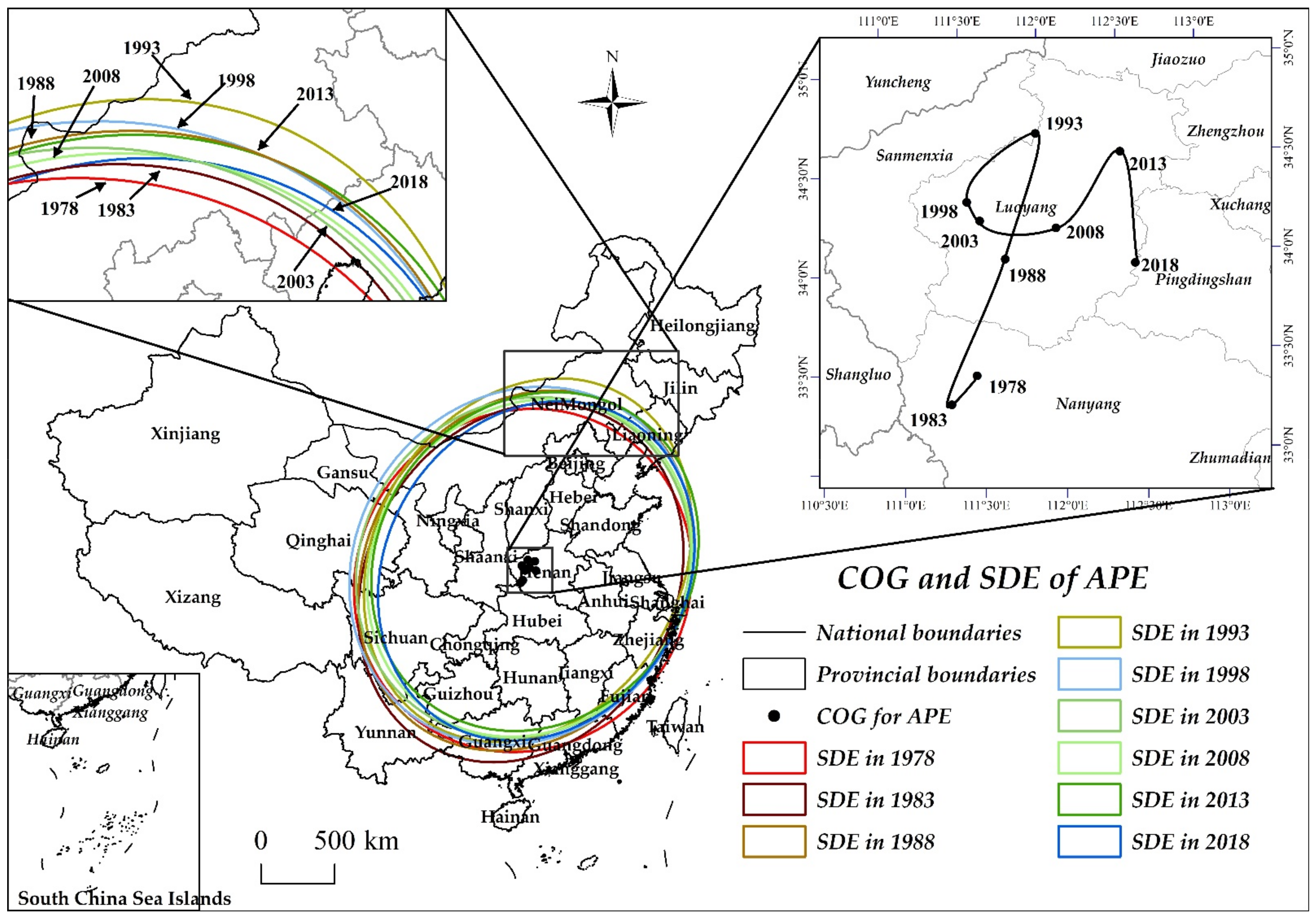
Under the dual constraints, the COG of APE transferred to the northeast, and the transfer path was with fluctuations. In the east-west direction, the transfer was eastward, and in the north-south direction, the transfer was northward, showing a northeast to southwest spatial pattern overall. The distance and speed of COG transfer showed the trend of increase, decrease, and slight increase. The changes in the SDE of APE were similar to those of COG transfer. The ellipse gradually shifted to the northeast and resembled less and less of a circle. The major axis was in the north-south direction and expanded, the minor axis was in the east-west direction and contracted, and the ellipse covered a gradually decreasing area. The spatial distribution of APE tended to be unbalanced in the east-west direction and tended to cluster in the north-south direction towards the east by north.

(3)

Under the dual constraints, APE showed significant spatial convergence characteristics. The gap between regions was narrowing, and the trend of latecomer catching-up was significant in the low APE regions. The spatial effect accelerated the convergence rate of APE and shortened the convergence period of APE to its own steady-state. The convergence rates of different regions showed a decreasing distribution pattern from the central and western regions, the northeastern region, and the eastern region. The latecomer advantage of the central and western regions was significant, and the marginal decreasing effect reduced the convergence rate of the eastern and northeastern regions. The APE convergence rates in different time periods had a phase change, which corresponded to the distance and speed of COG transfer.

References

1. IPCC. Summary for policymakers. In Global Warming of 1.5°; World Meteorological Organization: Geneva, Switzerland, 2018; 32p. [Google Scholar]
2. IPCC. Summary for Policymakers. In Climate Change 2021: The Physical Science Basis. Contribution of Working Group I to the Sixth Assessment Report of the Intergovernmental Panel on Climate Change; Cambridge University Press: Cambridge, UK, 2021. [Google Scholar]
3. Zhang, P.; Zhang, J.; Chen, M. Economic impacts of climate change on agriculture: The importance of additional climatic variables other than temperature and precipitation. J. Environ. Econ. Manag. 2017, 83, 8–31. [Google Scholar] [CrossRef]
4. Wang, J.X.; Mendelsohn, R.; Dinar, A.; Huang, J.K.; Zhang, L.J. The impact of climate change on china’s agriculture. Agric. Econ. 2010, 40, 323–337. [Google Scholar] [CrossRef]
5. Xie, L.Y.; Li, Y.; Qian, F.K.; Zhao, H.; Han, X.; Lin, E. Analysis on agricultural sensitivity and vulnerability to climate change and countermeasures. China Popul. Resour. Environ. 2014, 24, 25–30. [Google Scholar] [CrossRef]
6. Yin, C.J.; Li, G.C.; Fan, L.X.; Gao, X. Climate change, technology stocks and agricultural productivity growth. Chin. Rural. Econ. 2016, 5, 16–28. [Google Scholar]
7. Schmidhuber, J.; Tubiello, F.N. Global food security under climate change. Proc. Natl. Acad. Sci. USA 2007, 104, 19703–19708. [Google Scholar] [CrossRef] [Green Version]
8. Vermeulen, S.J.; Campbell, B.M.; Ingram, J.S. Climate change and food systems. Annu. Rev. Environ. Resour. 2012, 37, 195–222. [Google Scholar] [CrossRef] [Green Version]
9. Pan, G.X.; Gao, M.; Hu, G.H.; Wei, Q.P.; Yang, X.G.; Zhang, W.Z.; Zhou, G.S.; Zou, J.W. Issues and challenges on mitigation of climate change impacts on China’s future agriculture. J. Agro-Environ. Sci. 2011, 30, 1707–1712. [Google Scholar]
10. Liu, Y.; Wang, E.; Yang, X.G.; Wang, J. Contributions of climatic and crop varietal changes to crop production in the North China Plain, since 1980s. Glob. Change Biol. 2010, 16, 2287–2299. [Google Scholar] [CrossRef]
11. Liu, L.T.; Liu, X.J.; Lun, F. Research on China’s food security under global climate change background. J. Nat. Resour. 2018, 33, 927–939. [Google Scholar] [CrossRef] [Green Version]
12. Gao, M. Research on Agricultural Productivity in China from the climate change view. China Soft Sci. 2018, 9, 26–39. [Google Scholar]
13. Piao, S.; Ciais, P.; Huang, Y.; Shen, Z.; Peng, S.; Li, J.; Zhou, L.; Liu, H.; Ma, Y.; Ding, Y.; et al. The impacts of climate change on water resources and agriculture in China. Nature 2010, 467, 43–51. [Google Scholar] [CrossRef] [PubMed]
14. Guo, J.P. Advances in impacts of climate change on agricultural production in China. J. Appl. Meteorol. Sci. 2015, 26, 1–11. [Google Scholar] [CrossRef]
15. Cai, W.C.; Yang, H.Y.; Zhang, Q.Q.; Huo, X.X. Does part-time farming necessarily lead to low efficiency of agriculture production? From the perspective of agricultural social service. J. Arid Land Resour. Environ. 2022, 36, 26–32. [Google Scholar] [CrossRef]
16. Liu, Y.S.; Zou, L.L.; Wang, Y.S. Spatial-temporal characteristics and influencing factors of agricultural eco-efficiency in China in recent 40 years. Land Use Policy 2020, 97, 104794. [Google Scholar] [CrossRef]
17. Maxime, D.; Marcotie, M.; Arcand, Y. Development of eco-efficiency indicators for the Canadian food and beverage industry. J. Clean. Prod. 2006, 14, 636–648. [Google Scholar] [CrossRef]
18. Yang, X.; Shang, G.Y. Smallholders’ Agricultural Production Efficiency of Conservation Tillage in Jianghan Plain, China—Based on a Three-Stage DEA Model. Int. J. Environ. Res. Public Health 2020, 17, 7470. [Google Scholar] [CrossRef]
19. Pan, D.; Ying, R.Y. Agricultural eco-efficiency evaluation in China based on SBM model. Acta Ecol. Sin. 2013, 33, 3837–3845. [Google Scholar] [CrossRef] [Green Version]
20. He, P.P.; Zhang, J.B.; Li, W.J. The role of agricultural green production technologies in improving low-carbon efficiency in China: Necessary but not effective. J. Environ. Manag. 2021, 293, 112837. [Google Scholar] [CrossRef]
21. Wang, B.Y.; Zhang, W.G. A research of agricultural eco-efficiency measure in China and space-time differences. China Popul. Resour. Environ. 2016, 26, 11–19. [Google Scholar] [CrossRef]
22. Hou, M.Y.; Yao, S.B. Spatial-temporal evolution and trend prediction of agricultural eco-efficiency in China: 1978–2016. Acta Geogr. Sin. 2018, 73, 2168–2183. [Google Scholar] [CrossRef]
23. Wang, H.; Bian, Y.J. Agricultural production efficiency, agricultural carbon emission dynamics and threshold characteristics. J. Agrotech. Econ. 2015, 6, 36–47. [Google Scholar]
24. Yin, Z.Q.; Wu, J.Z. Spatial Dependence Evaluation of Agricultural Technical Efficiency—Based on the Stochastic Frontier and Spatial Econometric Model. Sustainability 2021, 13, 2708. [Google Scholar] [CrossRef]
25. Ma, X.D.; Sun, X.X. Space-time evolvement and problem area diagnosis of agriculture transformation development in Jiangsu Province since 2000—Based on a Total Factor Productivity perspective. Econ. Geogr. 2016, 36, 132–138. [Google Scholar] [CrossRef]
26. Zheng, D.F.; Hao, S.; Sun, C.Z. Evaluation of agricultural ecological efficiency and its spatial-temporal differentiation based on DEA-ESDA. Sci. Geogr. Sin. 2018, 38, 419–427. [Google Scholar] [CrossRef]
27. Barro, R.; Sala-i-Martin, X. Economic Growth; McGraw-Hill: New York, NY, USA, 1995. [Google Scholar]
28. Zhao, L.; Yang, X.Y.; Wang, H.M. Analysis on Convergence of Provincial Productivity in China’s Agriculture after Reform. Nankai Econ. Stud. 2007, 1, 107–116. [Google Scholar] [CrossRef]
29. Zeng, X.F.; Li, G.P. Estimate the agricultural production efficiencies and convergence:1980–2005. J. Quant. Tech. Econ. 2008, 8, 81–92. [Google Scholar] [CrossRef]
30. Tian, W.; Liu, S.W. Analysis on regional difference and convergence of agricultural technology efficiency in China. Issues Agric. Econ. 2012, 33, 11–18, 110. [Google Scholar] [CrossRef]
31. Gao, M.; Song, H.Y. Spatial convergences and difference between functional areas of grain production technical efficiency: Concurrently discuss ripple effect in technology diffusion. Manag. World 2014, 7, 83–92. [Google Scholar] [CrossRef]
32. Hou, M.Y.; Yao, S.B. Convergence and differentiation characteristics on agro-ecological efficiency in China from a spatial perspective. China Popul. Resour. Environ. 2019, 29, 116–126. [Google Scholar] [CrossRef]
33. Zhuang, X.H.; Li, Z.Y.; Zheng, R.; Na, S.Y.; Zhou, Y.L. Research on the Efficiency and Improvement of Rural Development in China: Based on Two-Stage Network SBM Model. Sustainability 2021, 13, 2914. [Google Scholar] [CrossRef]
34. Tone, K. A slacks-based measure of efficiency in data envelopment analysis. Eur. J. Oper. Res. 2001, 130, 498–509. [Google Scholar] [CrossRef] [Green Version]
35. Tone, K. A slacks-based measure of super-efficiency in data envelopment analysis. Eur. J. Oper. Res. 2002, 143, 32–41. [Google Scholar] [CrossRef] [Green Version]
36. Xu, J.; Zhu, C.L. A study on economic growth efficiency under resources and environment constraints in ethnic minority regions. J. Quant. Tech. Econ. 2018, 35, 95–110. [Google Scholar] [CrossRef]
37. Ye, A.Z. Non-Parametric Econometrics; Nankai University Press: Tianjin, China, 2005. [Google Scholar]
38. Lefever, D. Measuring geographic concentration by means of the Standard Deviational Ellipse. Am. J. Sociol. 1926, 32, 88–94. [Google Scholar] [CrossRef]
39. Furfey, P. A note on Lefever’s “Standard Deviational Ellipse”. Am. J. Sociol. 1927, 33, 94–98. [Google Scholar] [CrossRef]
40. Zhao, L.; Zhao, Z.Q. Spatial Agglomeration of the manufacturing industry in China. J. Quant. Tech. Econ. 2014, 31, 110–121, 138. [Google Scholar] [CrossRef]
41. Zhao, L.; Zhao, Z.Q. Projecting the spatial variation of economic based on the specific ellipses in China. Sci. Geogr. Sin. 2014, 34, 979–986. [Google Scholar] [CrossRef]
42. Sun, C.Z.; Ma, Q.F.; Zhao, L.S. Temporal and spatial evolution of green efficiency of water resources in China and its convergence analysis. Prog. Geogr. 2018, 37, 901–911. [Google Scholar] [CrossRef]
43. Fan, Q.; Hudson, D. A new endogenous spatial temporal weight matrix based on ratios of Global Moran’s I. J. Quant. Tech. Econ. 2018, 35, 131–149. [Google Scholar] [CrossRef]
44. Hong, G.Z.; Hu, H.Y.; Li, X. Analysis of Regional Growth Convergence with Spatial Econometrics in China. Acta Geogr. Sin. 2010, 65, 1548–1558. [Google Scholar] [CrossRef]
45. Shi, C.L.; Li, Y.; Zhu, J.F. Rural labor transfer, excessive fertilizer use and agricultural non-point source pollution. J. China Agric. Univ. 2016, 21, 169–180. [Google Scholar] [CrossRef]
46. Lai, S.Y.; Du, P.F.; Chen, J.N. Evaluation of non-point source pollution based on unit analysis. J. Tsinghua Univ. 2004, 9, 1184–1187. [Google Scholar] [CrossRef]
47. Wu, X.Q.; Wang, Y.P.; He, T.M.; Lu, G.F. Agricultural eco-efficiency evaluation based on AHP and DEA Model. Resour. Environ. Yangtze Basin 2012, 21, 714–719. [Google Scholar]
48. Li, B.; Zhang, J.B.; Li, H.P. Research on spatial-temporal characteristics and affecting factors decomposition of agricultural carbon emission in China. China Popul. Resour. Environ. 2011, 21, 80–86. [Google Scholar] [CrossRef]
49. Xu, X.X.; Shu, Y. Growth dynamics in Chinese provinces (1978–1998). China Econ. Q. 2004, 2, 619–638. [Google Scholar] [CrossRef]
50. Liang, H.Y. Distribution dynamics, difference decomposition and convergence mechanism of producer services industry in Chinese urban clusters. J. Quant. Tech. Econ. 2018, 35, 40–60. [Google Scholar] [CrossRef]
51. Yu, Y.Z. Dynamic spatial convergence of provincial total factor productivity in China. J. World Econ. 2015, 38, 30–55. [Google Scholar]
52. Yang, M.H.; Zhang, H.X.; Sun, Y.N.; Li, Q.Q. The study of the science and technology innovation ability in eight comprehensive economic areas of China. J. Quant. Tech. Econ. 2018, 35, 3–19. [Google Scholar] [CrossRef]
53. Elhorst, J.P. Dynamic spatial panels: Models, methods, and inferences. J. Geogr. Syst. 2012, 14, 5–28. [Google Scholar] [CrossRef]
54. Hu, C.; Wei, Y.Y.; Hu, W. Research on the relationship between agricultural policy, technological innovation and agricultural carbon emissions. Issues Agric. Econ. 2018, 9, 66–75. [Google Scholar] [CrossRef]
55. Zhang, D.H.; Wang, H.Q.; Lou, S.; Zhong, S. Research on grain production efficiency in China’s main grain producing areas from the perspective of financial support. PLoS ONE 2021, 16, e0247610. [Google Scholar] [CrossRef]
56. Cui, Y.; Liu, W.X.; Khan, S.U.; Cai, Y.; Zhu, J.; Deng, Y.; Zhao, M.J. Regional differential decomposition and convergence of rural green development efficiency: Evidence from China. Environ. Sci. Pollut. Res. 2020, 27, 22364–22379. [Google Scholar] [CrossRef]
57. Chen, S.; Gong, B.L. Response and adaptation of agriculture to climate change: Evidence from China. J. Dev. Econ. 2021, 148, 102557. [Google Scholar] [CrossRef]
58. Zhang, L.X.; Bai, Y.L.; Sun, M.X.; Xu, X.B.; He, J.L. Views on agricultural green production from perspective of system science. Issues Agric. Econ. 2021, 10, 42–50. [Google Scholar] [CrossRef]
59. Chen, L.; Friedland, S. The tensor rank of tensor product of two three-qubit W states is eight. Linear Algebra Its Appl. 2018, 543, 1–16. [Google Scholar] [CrossRef] [Green Version]
60. Tomal, M.; Gumieniak, A. Agricultural land price convergence: Evidence from Polish provinces. Agriculture 2020, 10, 183. [Google Scholar] [CrossRef]
61. Deng, X.; Li, Z.; Gibson, J. A review on trade-off analysis of ecosystem services for sustainable land-use management. J. Geogr. Sci. 2016, 26, 953–968. [Google Scholar] [CrossRef] [Green Version]
62. Liu, Z.J.; Liu, Y.S.; Li, Y. Anthropogenic contributions dominate trends of vegetation cover change over the farming-pastoral ecotone of northern china. Ecol. Indic. 2018, 95, 370–378. [Google Scholar] [CrossRef]
63. Ma, L.; Long, H.L.; Tang, L.S.; Tu, S.; Zhang, Y.; Qu, Y. Analysis of the spatial variations of determinants of agricultural production efficiency in China. Comput. Electron. Agric. 2021, 180, 105890. [Google Scholar] [CrossRef]
64. Guo, Y.; Wang, J. Spatiotemporal changes of chemical fertilizer application and its environmental risks in China from 2000 to 2019. Int. J. Environ. Res. Public Health 2021, 18, 11911. [Google Scholar] [CrossRef]
65. Liu, J.; Dong, C.; Liu, S.; Rahman, S.; Sriboonchitta, S. Sources of total-factor productivity and efficiency changes in China’s agriculture. Agriculture 2020, 10, 279. [Google Scholar] [CrossRef]
66. Hou, M.Y.; Deng, Y.J.; Yao, S.B. Coordinated relationship between urbanization and grain production in China: Degree measurement, spatial differentiation and its factors detection. J. Clean. Prod. 2022, 331, 129957. [Google Scholar] [CrossRef]
Figure 1. The trend of APE under dual constraints during 1978–2018.
Agriculture 12 00116 g001
Figure 2. The KDE of APE under climate change during 1978–2018. (a) is the kernel density estimation at the national level; (b) is the kernel density estimation of the eastern region; (c) is the kernel density estimation of the central region; (d) is the kernel density estimation of the western region; (e) is the kernel density estimation of the northeastern region.
Agriculture 12 00116 g002aAgriculture 12 00116 g002b
Figure 3. Changes of the COG and SDE of APE in China since 1978.
Agriculture 12 00116 g003