
Input Use Efficiency Management for Paddy Production Systems in India: A Machine Learning Approach

 ,
, 
 ,
, 
 , and
, and 
Abstract
:1. Introduction
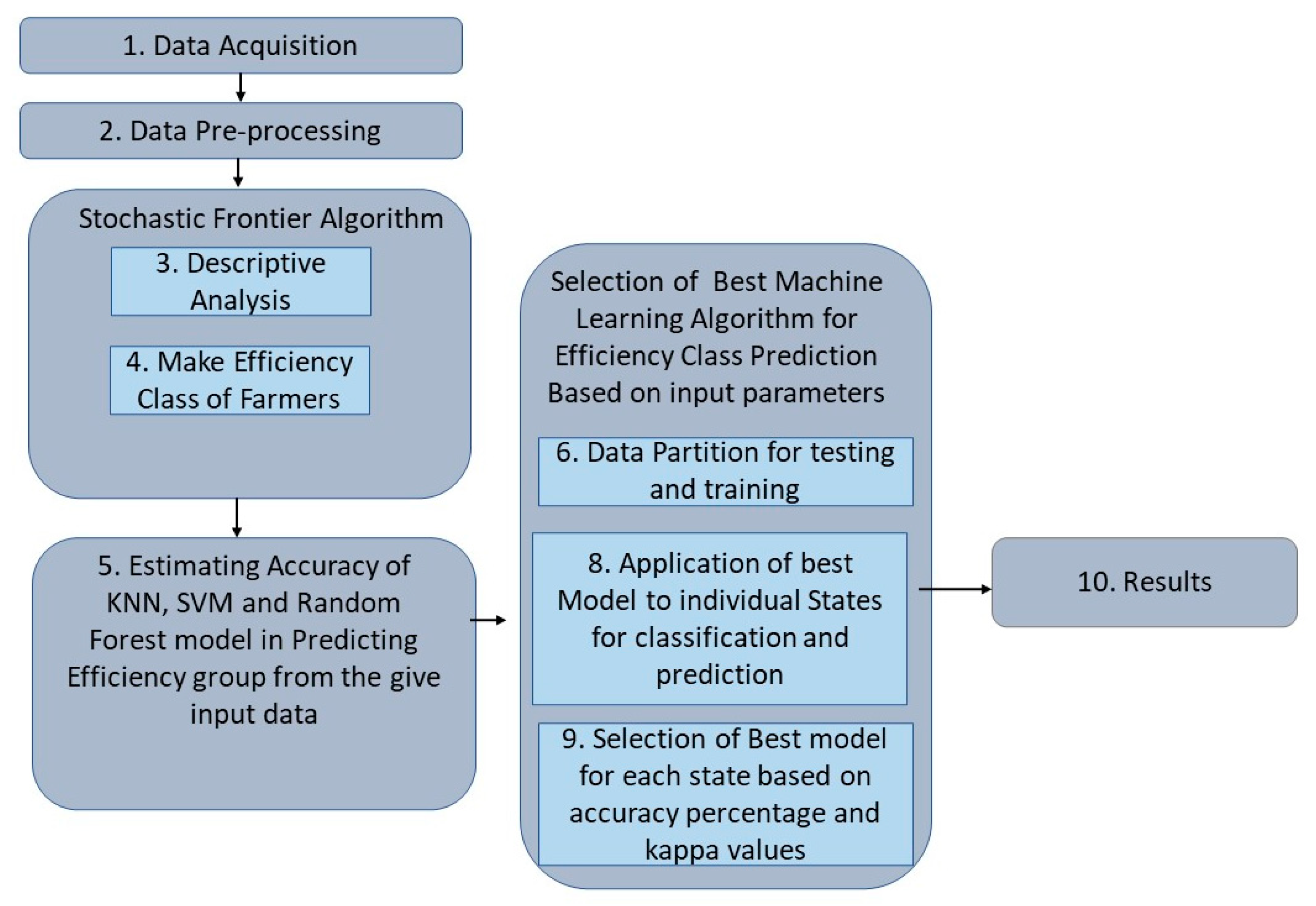
2. Data and Methodology
2.1. Data Acquisition
2.2. Data Pre-Processing
2.3. Stochastic Frontier Algorithm
- Y = the yield or any variable representing the productivity per unit area.
- Xi = the vector of inputs used in production.
- βi = the estimated coefficient of the ith input.
- u = the error term.
- Y = the yield or any variable representing the productivity per unit.
- Xi = the vector of inputs (the same as Equation (1));
- βi = the estimated coefficient of the ith input.
- vi = an asymmetrical random term or stochastic noise, assumed with a normal distribution
- ui = the individual farm level technical inefficiency assumed to be half-normally distributed.
- Yi= Output/Yield (quintals per hectare)
- X1 = Total human labor (Man-hours)
- X2 = Total animal labor (Hours)
- X3 = Total machine labor (Hours)
- X4 = Total Fertilizer (kg.)
- X5 = Total insecticide (Rupees).
- f = the Cobb–Douglas type production function.
- TE = the technical efficiency of an individual farm (0 < TEi ≤ 1).
2.4. Machine Learning Algorithms for the Prediction of Efficiency Classes
3. Results and Discussion
3.1. The Status of Paddy Farming in India
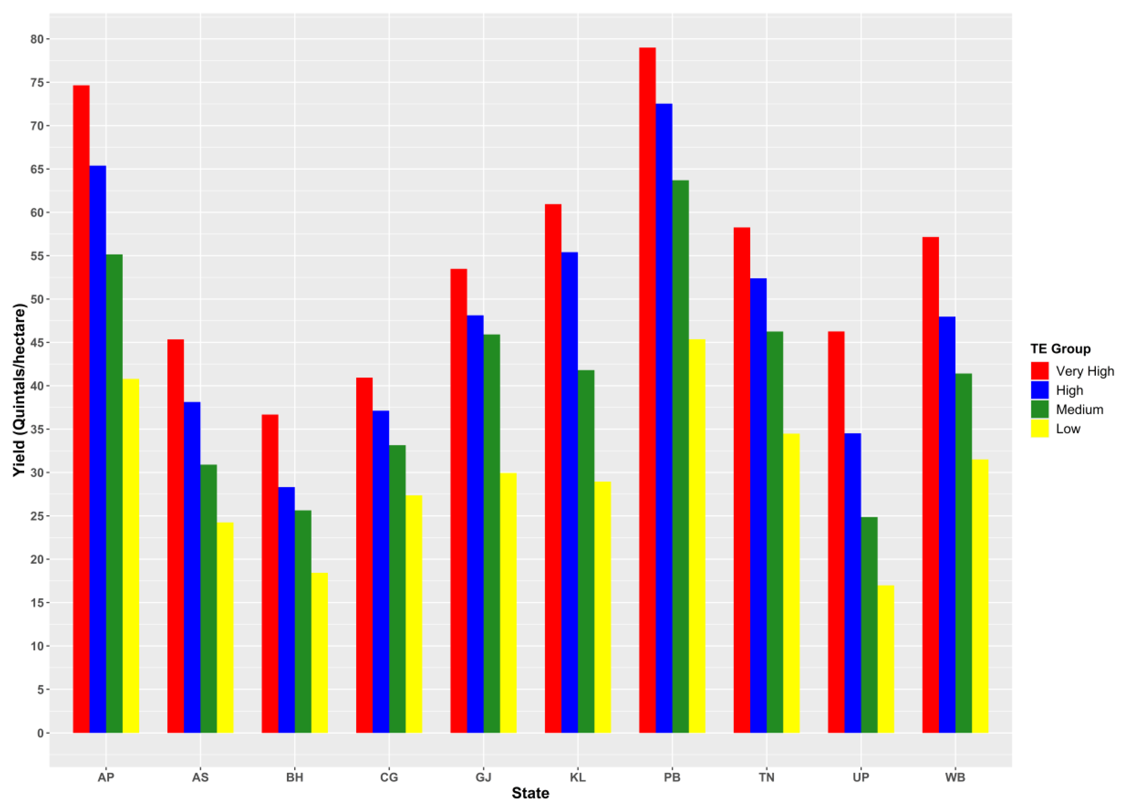
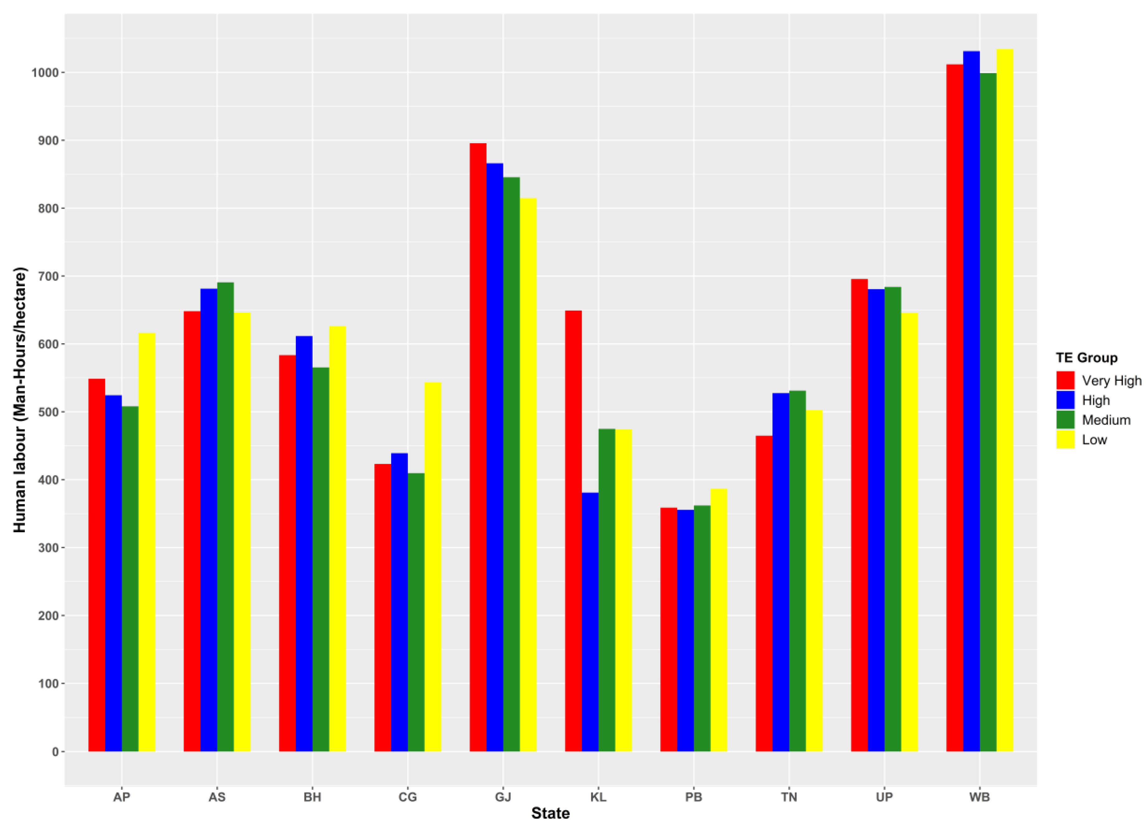
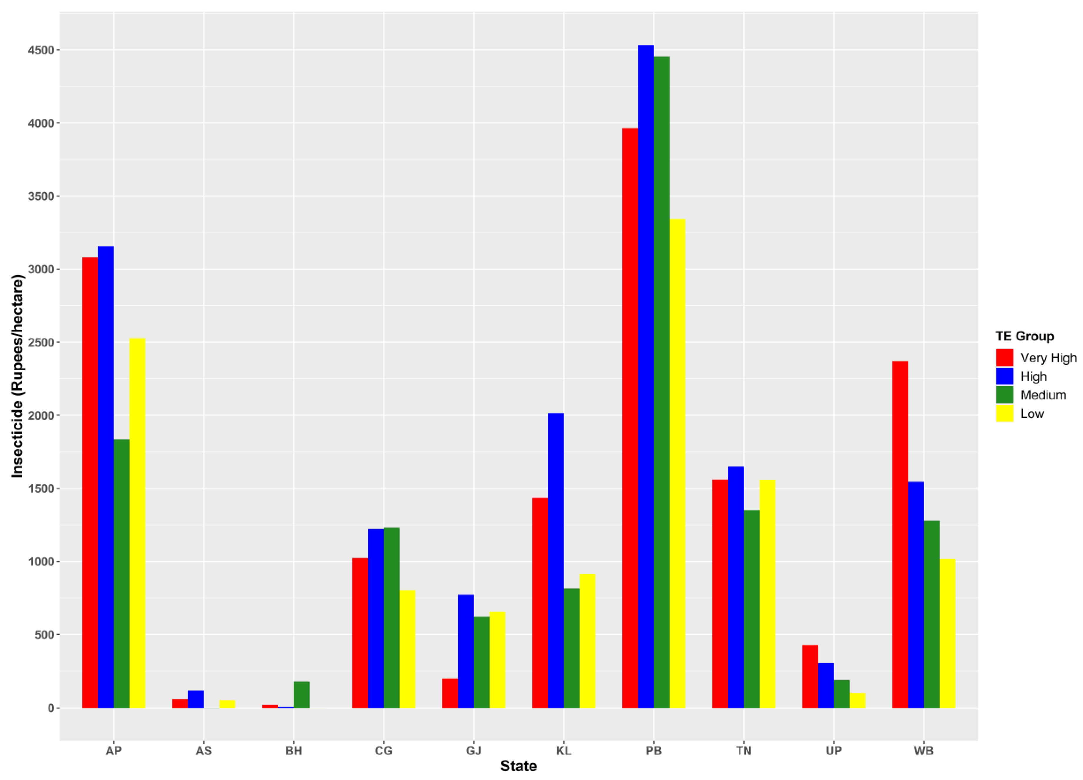
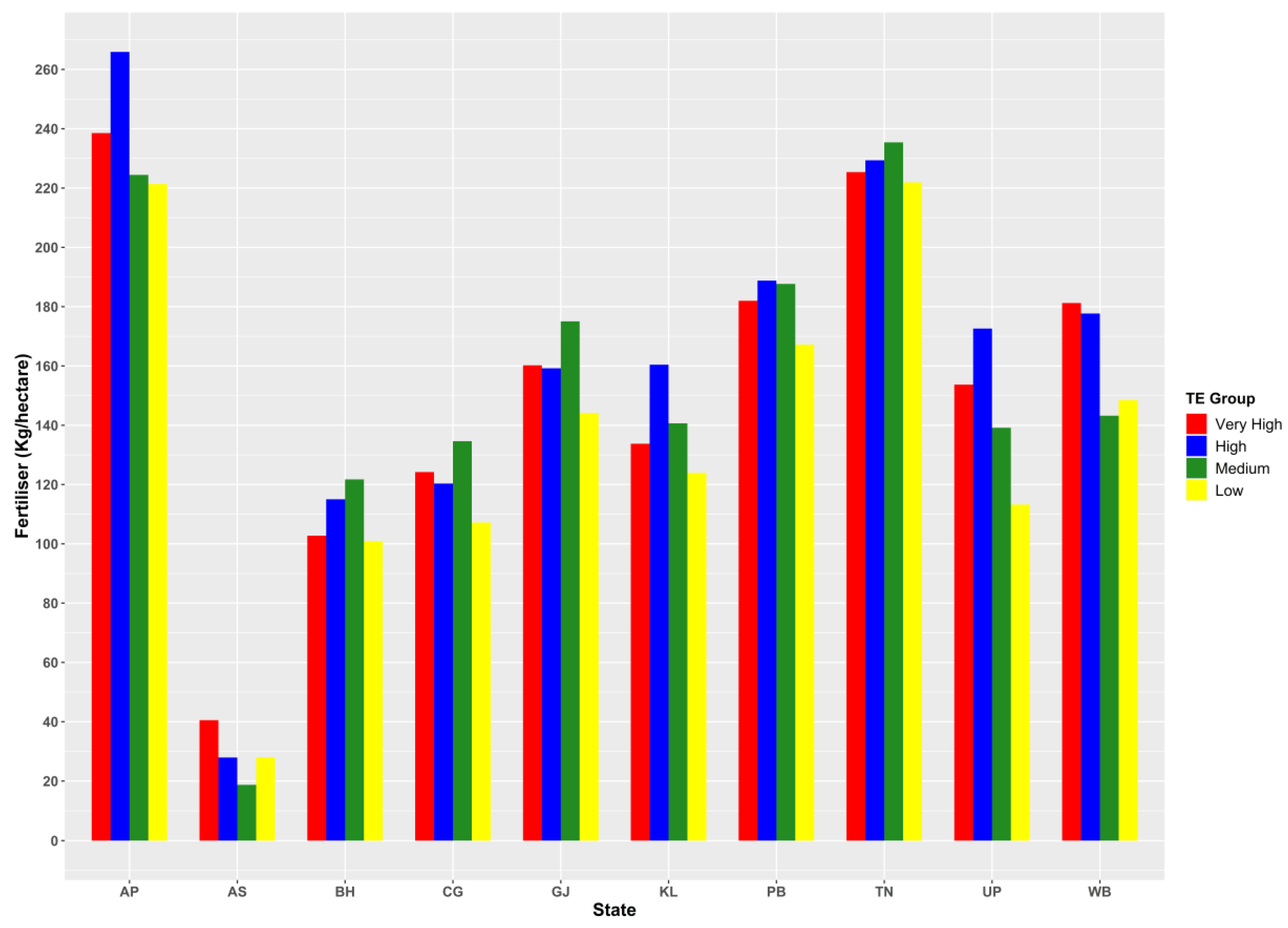
3.2. Regional Disparity in Productivity and Input Use
3.3. The Stochastic Frontier Approach of Technical Efficiency Estimation
3.4. Machine Learning Models for Efficiency Group Prediction
4. Conclusions
Author Contributions
Funding
Institutional Review Board Statement
Informed Consent Statement
Data Availability Statement
Conflicts of Interest
Appendix A

| State | Punjab | |||||||||||
|---|---|---|---|---|---|---|---|---|---|---|---|---|
| Model | KNN | SVM | RF | |||||||||
| Class | Low TE | Medium TE | High TE | Very High TE | Low TE | Medium TE | High TE | Very High TE | Low TE | Medium TE | High TE | Very High TE |
| Precision | 0.167 | 0.770 | 0.190 | 0.455 | 0.900 | 0.969 | 0.667 | 0.936 | 0.900 | 0.985 | 0.800 | 0.968 |
| Recall | 0.100 | 0.877 | 0.267 | 0.484 | 1.000 | 0.710 | 0.979 | 0.825 | 0.976 | 0.710 | 0.979 | 0.947 |
| Sensitivity | 0.100 | 0.877 | 0.267 | 0.484 | 1.000 | 0.875 | 0.909 | 0.744 | 0.900 | 0.877 | 0.923 | 0.909 |
| Specificity | 0.881 | 0.452 | 0.638 | 0.684 | 0.900 | 0.969 | 0.667 | 0.936 | 0.900 | 0.985 | 0.800 | 0.968 |
| State | Andhra Pradesh | |||||||||||
| Model | KNN | SVM | RF | |||||||||
| Class | Low TE | Medium TE | High TE | Very High TE | Low TE | Medium TE | High TE | Very High TE | Low TE | Medium TE | High TE | Very High TE |
| Precision | NA | 0.508 | 0.682 | 0.000 | NA | 0.855 | 0.864 | 0.200 | NA | 0.873 | 0.864 | 0.600 |
| Recall | NA | 0.564 | 0.682 | 0.000 | 1.000 | 0.823 | 0.741 | 0.842 | 0.987 | 0.919 | 0.889 | 0.790 |
| Sensitivity | NA | 0.564 | 0.682 | 0.000 | NA | 0.810 | 0.731 | 0.250 | 0.000 | 0.906 | 0.864 | 0.429 |
| Specificity | 1.000 | 0.516 | 0.741 | 0.947 | NA | 0.855 | 0.864 | 0.200 | NA | 0.873 | 0.864 | 0.600 |
| States | Assam | |||||||||||
| Model | KNN | SVM | RF | |||||||||
| Class | Low TE | Medium TE | High TE | Very High TE | Low TE | Medium TE | High TE | Very High TE | Low TE | Medium TE | High TE | Very High TE |
| Precision | 0.536 | 0.333 | 1.000 | 0.000 | 0.871 | 0.818 | 0.000 | 0.000 | 0.903 | 0.818 | 1.000 | 0.400 |
| Recall | 0.484 | 0.273 | 0.333 | 0.000 | 0.957 | 0.869 | 1.000 | 1.000 | 0.957 | 0.967 | 1.000 | 1.000 |
| Sensitivity | 0.484 | 0.273 | 0.333 | 0.000 | 0.931 | 0.692 | NA | NA | 0.933 | 0.900 | 1.000 | 1.000 |
| Specificity | 0.723 | 0.803 | 1.000 | 0.864 | 0.871 | 0.818 | 0.000 | 0.000 | 0.903 | 0.818 | 1.000 | 0.400 |
| States | Bihar | |||||||||||
| Model | KNN | SVM | RF | |||||||||
| Class | Low TE | Medium TE | High TE | Very High TE | Low TE | Medium TE | High TE | Very High TE | Low TE | Medium TE | High TE | Very High TE |
| Precision | 0.111 | 0.529 | 0.300 | 0.000 | 0.500 | 0.773 | 0.467 | 0.538 | 0.667 | 0.727 | 0.800 | 0.846 |
| Recall | 0.083 | 0.409 | 0.200 | 0.000 | 0.875 | 0.987 | 0.787 | 1.000 | 0.900 | 1.000 | 0.766 | 1.000 |
| Sensitivity | 0.083 | 0.409 | 0.200 | 0.000 | 0.546 | 0.944 | 0.412 | 1.000 | 0.667 | 1.000 | 0.522 | 1.000 |
| Specificity | 0.800 | 0.892 | 0.851 | 0.987 | 0.500 | 0.773 | 0.467 | 0.538 | 0.667 | 0.727 | 0.800 | 0.846 |
| States | Chhattisgarh | |||||||||||
| Model | KNN | SVM | RF | |||||||||
| Class | Low TE | Medium TE | High TE | Very High TE | Low TE | Medium TE | High TE | Very High TE | Low TE | Medium TE | High TE | Very High TE |
| Precision | 0.200 | 0.455 | 0.227 | 0.286 | 0.500 | 0.688 | 0.650 | 0.500 | 0.625 | 0.938 | 0.700 | 0.625 |
| Recall | 0.125 | 0.313 | 0.250 | 0.250 | 0.977 | 0.985 | 0.897 | 0.684 | 0.977 | 0.955 | 0.956 | 0.895 |
| Sensitivity | 0.125 | 0.313 | 0.250 | 0.250 | 0.667 | 0.917 | 0.650 | 0.400 | 0.714 | 0.833 | 0.824 | 0.714 |
| Specificity | 0.955 | 0.910 | 0.750 | 0.737 | 0.500 | 0.688 | 0.650 | 0.500 | 0.625 | 0.938 | 0.700 | 0.625 |
| States | Gujarat | |||||||||||
| Model | KNN | SVM | RF | |||||||||
| Class | Low TE | Medium TE | High TE | Very High TE | Low TE | Medium TE | High TE | Very High TE | Low TE | Medium TE | High TE | Very High TE |
| Precision | NA | 0.535 | 0.438 | 0.250 | 0.000 | 0.900 | 0.833 | 0.286 | 0.000 | 0.833 | 0.917 | 0.714 |
| Recall | 0.000 | 0.767 | 0.583 | 0.286 | 1.000 | 0.830 | 0.969 | 0.700 | 1.000 | 0.906 | 0.922 | 0.900 |
| Sensitivity | 0.000 | 0.767 | 0.583 | 0.286 | 0.750 | 0.909 | 0.250 | NA | 0.833 | 0.815 | 0.714 | |
| Specificity | 1.000 | 0.623 | 0.719 | 0.700 | 0.000 | 0.900 | 0.833 | 0.286 | 0.000 | 0.833 | 0.917 | 0.714 |
| States | Kerala | |||||||||||
| Model | KNN | SVM | RF | |||||||||
| Class | Low TE | Medium TE | High TE | Very High TE | Low TE | Medium TE | High TE | Very High TE | Low TE | Medium TE | High TE | Very High TE |
| Precision | 0.638 | 0.273 | 0.444 | 0.556 | 0.952 | 0.600 | 0.692 | 0.714 | 0.952 | 1.000 | 0.846 | 1.000 |
| Recall | 0.714 | 0.200 | 0.615 | 0.714 | 0.778 | 1.000 | 0.889 | 0.800 | 0.889 | 1.000 | 0.917 | 0.800 |
| Sensitivity | 0.714 | 0.200 | 0.615 | 0.714 | 0.833 | 1.000 | 0.692 | 0.556 | 0.909 | 1.000 | 0.786 | 0.636 |
| Specificity | 0.528 | 0.882 | 0.722 | 0.800 | 0.952 | 0.600 | 0.692 | 0.714 | 0.952 | 1.000 | 0.846 | 1.000 |
| States | Tamil Nadu | |||||||||||
| Model | KNN | SVM | RF | |||||||||
| Class | Low TE | Medium TE | High TE | Very High TE | Low TE | Medium TE | High TE | Very High TE | Low TE | Medium TE | High TE | Very High TE |
| Precision | 0.000 | 0.393 | 0.125 | NA | 0.200 | 0.786 | 0.455 | 0.000 | 0.600 | 0.893 | 0.455 | 1.000 |
| Recall | 0.000 | 0.393 | 0.091 | 0.000 | 1.000 | 0.978 | 0.868 | 1.000 | 1.000 | 0.966 | 0.868 | 1.000 |
| Sensitivity | 0.000 | 0.393 | 0.091 | 0.000 | 1.000 | 0.917 | 0.500 | NA | 1.000 | 0.893 | 0.500 | 1.000 |
| Specificity | 0.959 | 0.809 | 0.816 | 1.000 | 0.200 | 0.786 | 0.455 | 0.000 | 0.600 | 0.893 | 0.455 | 1.000 |
| States | Uttar Pradesh | |||||||||||
| Model | KNN | SVM | RF | |||||||||
| Class | Low TE | Medium TE | High TE | Very High TE | Low TE | Medium TE | High TE | Very High TE | Low TE | Medium TE | High TE | Very High TE |
| Precision | 0.353 | 0.333 | 0.320 | 0.682 | 0.333 | 0.875 | 0.684 | 0.867 | 0.733 | 1.000 | 0.474 | 0.800 |
| Recall | 0.400 | 0.313 | 0.421 | 1.000 | 0.757 | 0.980 | 0.558 | 0.333 | 0.811 | 0.960 | 0.907 | 0.778 |
| Sensitivity | 0.400 | 0.313 | 0.421 | 1.000 | 0.357 | 0.875 | 0.406 | 0.684 | 0.611 | 0.800 | 0.692 | 0.857 |
| Specificity | 0.703 | 0.901 | 0.605 | 0.222 | 0.333 | 0.875 | 0.684 | 0.867 | 0.733 | 1.000 | 0.474 | 0.800 |
| States | West Bengal | |||||||||||
| Model | KNN | SVM | RF | |||||||||
| Class | Low TE | Medium TE | High TE | Very High TE | Low TE | Medium TE | High TE | Very High TE | Low TE | Medium TE | High TE | Very High TE |
| Precision | 0.300 | 0.385 | 0.333 | 0.000 | 0.467 | 0.667 | 0.077 | 0.000 | 0.667 | 0.667 | 0.846 | 0.000 |
| Recall | 0.400 | 0.278 | 0.154 | 0.000 | 0.703 | 0.929 | 0.980 | 0.952 | 0.946 | 0.960 | 0.959 | 0.905 |
| Sensitivity | 0.400 | 0.278 | 0.154 | 0.000 | 0.389 | 0.632 | 0.500 | 0.000 | 0.833 | 0.750 | 0.846 | 0.000 |
| Specificity | 0.622 | 0.919 | 0.918 | 0.952 | 0.467 | 0.667 | 0.077 | 0.000 | 0.667 | 0.667 | 0.846 | 0.000 |
| Abbreviation | State Name |
|---|---|
| AP | Andhra Pradesh |
| AS | Assam |
| BH | Bihar |
| CG | Chhattisgarh |
| GJ | Gujarat |
| KL | Kerala |
| PB | Punjab |
| TN | Tamil Nadu |
| UP | Uttar Pradesh |
| WB | West Bengal |
| Abbreviation | Full Form |
|---|---|
| TE | Technical Efficiency |
| DES | Department of Economics and Statistics |
| CACP | Commission for Agricultural Cost and Prices |
| FAO | Food and Agriculture Organization |
| KNN | K- Nearest Neighbor |
| SVM | Support Vector Machine |
| RF | Random Forest |
| ANN | Artificial Neural Network |
| MLR | Multiple Linear Regression |
| SVR | Support Vector Regression |
| MANN | Modular Artificial Neural Networks |
| RGB | Red, Green, Blue |
| UAV | Unmanned Aerial Vehicle |
References
- Bacco, M.; Barsocchi, P.; Ferro, E.; Gotta, A.; Ruggeri, M. The Digitisation of Agriculture: A Survey of Research Activities on Smart Farming. Array 2019, 3–4, 100009. [Google Scholar] [CrossRef]
- FAO. AQUASTAT Core Database; Food and Agriculture Organization of the United Nations: Rome, Italy, 2018. [Google Scholar]
- Handbook of Indian Economy; Reserve Bank of India Publications: Mumbai, India, 2018.
- Singh, S. A study on technical efficiency of wheat cultivation in Haryana. Agric. Econ. Res. Rev. 2007, 20, 127–136. [Google Scholar]
- Gurjar, M.L.; Varghese, K.A. Structural Changes over Time in Cost of Cultivation of Major Rabi Crops in Rajasthan. Indian J. Agric. Econ. 2005, 60, 249–263. [Google Scholar]
- Narayanamoorthy, A. Profitability in crops cultivation in India: Some evidence from cost of cultivation survey data. Indian J. Agric. Econ. 2013, 68, 104–121. [Google Scholar]
- Guptha, C.; Raghu, P.T.; Aditi, N.; Kalaiselvan, N.N. Comparative trend analysis in cost of paddy cultivation in profitability across three states of India. Eur. Sci. J. 2014, 271. [Google Scholar] [CrossRef]
- Reddy, E.L.; Reddy, D.R. A Study on Resource use Efficiency of Agricultural Input Factors with Reference to Farm Size in Three Revenue Mandals of Nellore District: Andhra Pradesh. Glob. J. Manag. Bus. Res. 2014, 17, 48–55. [Google Scholar]
- Kalamkar, S.S.; Narayanamoorthy, A. Impact of Liberalisation on Domestic Agricultural Prices and Farm Income: An Analysis across States and Crops. Indian J. Agric. Econ. 2003, 58, 353–364. [Google Scholar]
- Narayanamoorthy, A. Relief Package for farmers: Can it stop suicides? Econ. Polit. Wkly. 2006, 41, 3353–3355. [Google Scholar]
- Narayanamoorthy, A. Deceleration in Agricultural Growth: Technology Fatigue or Policy Fatigue? Econ. Polit. Wkly. 2007, 42, 2375–2379. [Google Scholar]
- Sainath, P. Farm Suicides: A 12-Year Saga. The Hindu, 25 January 2010. [Google Scholar]
- Ali, M.; Chaudhry, M.A. Inter-Regional Farm Efficiency in Pakistan’s Punjab: A Frontier Production Function Study. J. Agric. Econ. 1990, 41, 62–74. [Google Scholar] [CrossRef]
- Umesh, K.B.; Bisaliah, S. Efficiency of groundnut production in Karnataka: Frontier profit function approach. Indian J. Agric. Econ. 1991, 46, 20–33. [Google Scholar]
- Gaddi, G.M.; Mundinasmani, S.M.; Hiremath, G.K. Resource use efficiency in groundnut production in Karnataka—An economic analysis. Agric. Situat. India 2002, 58, 517–522. [Google Scholar]
- KalirajanK, P.; Shand, R.T. A generalized measure of technical efficiency. Appl. Econ. 1989, 21, 25–34. [Google Scholar] [CrossRef]
- Kalirajan, K.; Obwona, M.; Zhao, S. A Decomposition of Total Factor Productivity Growth: The Case of Chinese Agricultural Growth before and after Reforms. Am. J. Agric. Econ. 1996, 78, 331–338. [Google Scholar] [CrossRef]
- Shanmugam, K.R.; Venkataramani, A. Technical Efficiency in Agricultural Production and Its Determinants: An Exploratory Study at the District Level; Madras School of Economics: Tamil Nadu, India, 2006; Volume 10. [Google Scholar]
- Zecca, F. The Use of Internet of Things for the Sustainability of the Agricultural Sector: The Case of Climate Smart Agriculture. Int. J. Civ. Eng. Technol. 2019, 10, 494–501. [Google Scholar]
- Helfer, G.A.; Victória Barbosa, J.L.; dos Santos, R.; da Costa, A. Ben A computational model for soil fertility prediction in ubiquitous agriculture. Comput. Electron. Agric. 2020, 175, 105602. [Google Scholar] [CrossRef]
- Ge, X.; Wang, J.; Ding, J.; Cao, X.; Zhang, Z.; Liu, J.; Li, X. Combining UAV-based hyperspectral imagery and machine learning algorithms for soil moisture content monitoring. PeerJ 2019, 7, e6926. [Google Scholar] [CrossRef]
- Yamaç, S.S.; Şeker, C.; Negiş, H. Evaluation of machine learning methods to predict soil moisture constants with different combinations of soil input data for calcareous soils in a semi arid area. Agric. Water Manag. 2020, 234, 106121. [Google Scholar] [CrossRef]
- Sanuade, O.A.; Hassan, A.M.; Akanji, A.O.; Olaojo, A.A.; Oladunjoye, M.A.; Abdulraheem, A. New empirical equation to estimatethe soil moisture content based on thermal properties using machine learning techniques. Arab. J. Geosci. 2020, 13, 377. [Google Scholar] [CrossRef]
- Helfer, G.; Barbosa, J.; Alves, D.; da Costa, A.; Beko, M.; Leithardt, V. Multispectral Cameras and Machine Learning Integrated into Portable Devices as Clay Prediction Technology. J. Sens. Actuator Netw. 2021, 10, 40. [Google Scholar] [CrossRef]
- Martini, B.; Helfer, G.; Barbosa, J.; Modolo, R.E.; da Silva, M.; de Figueiredo, R.; Mendes, A.; Silva, L.; Leithardt, V. IndoorPlant: A Model for Intelligent Services in Indoor Agriculture Based on Context Histories. Sensors 2021, 21, 1631. [Google Scholar] [CrossRef]
- Ramesh, S.; Vydeki, D. Recognition and classification of paddy leaf diseases using Optimized Deep Neural network with Jaya algorithm. Inf. Process. Agric. 2020, 7, 249–260. [Google Scholar] [CrossRef]
- Li, D.; Wang, R.; Xie, C.; Liu, L.; Zhang, J.; Li, R.; Wang, F.; Zhou, M.; Liu, W. A Recognition Method for Rice Plant Diseases and Pests Video Detection Based on Deep Convolutional Neural Network. Sensors 2020, 20, 578. [Google Scholar] [CrossRef] [Green Version]
- He, Y.; Zhou, Z.; Tian, L.; Liu, Y.; Luo, X. Brown rice planthopper (Nilaparvata lugens Stal) detection based on deep learning. Precis. Agric. 2020, 21, 1385–1402. [Google Scholar] [CrossRef]
- Huang, H.; Deng, J.; Lan, Y.; Yang, A.; Deng, X.; Wen, S.; Zhang, H.; Zhang, Y. Accurate Weed Mapping and Prescription Map Generation Based on Fully Convolutional Networks Using UAV Imagery. Sensors 2018, 18, 3299. [Google Scholar] [CrossRef] [PubMed] [Green Version]
- Dadashzadeh, M.; Abbaspour-Gilandeh, Y.; Mesri-Gundoshmian, T.; Sabzi, S.; Hernández-Hernández, J.L.; Hernández-Hernández, M.; Arribas, J.I. Weed Classification for Site-Specific Weed Management Using an Automated Stereo Computer-Vision Machine-Learning System in Rice Fields. Plants 2020, 9, 559. [Google Scholar] [CrossRef]
- Shidnal, S.; Latte, M.V.; Kapoor, A. Crop yield prediction: Two-tiered machine learning model approach. Int. J. Inf. Technol. 2019, 1–9. [Google Scholar] [CrossRef]
- Yang, Q.; Shi, L.; Han, J.; Zha, Y.; Zhu, P. Deep convolutional neural networks for rice grain yield estimation at the ripening stage using UAV-based remotely sensed images. Field Crop. Res. 2019, 235, 142–153. [Google Scholar] [CrossRef]
- Wan, L.; Cen, H.; Zhu, J.; Zhang, J.; Zhu, Y.; Sun, D.; Du, X.; Zhai, L.; Weng, H.; Li, Y.; et al. Grain yield prediction of rice using multi-temporal UAV-based RGB and multispectral images and model transfer—A case study of small farmlands in the South of China. Agric. For. Meteorol. 2020, 291, 108096. [Google Scholar] [CrossRef]
- Son, N.T.; Chen, C.F.; Chen, C.R.; Guo, H.Y.; Cheng, Y.S.; Chen, S.L.; Lin, H.S.; Chen, S.H. Machine learning approaches for rice crop yield predictions using time-series satellite data in Taiwan. Int. J. Remote Sens. 2020, 41, 7868–7888. [Google Scholar] [CrossRef]
- Amaratunga, V.; Wickramasinghe, L.; Perera, A.; Jayasinghe, J.; Rathnayake, U. Artificial Neural Network to Estimate the Paddy Yield Prediction Using Climatic Data. Math. Probl. Eng. 2020, 2020, 8627824. [Google Scholar] [CrossRef]
- Khosla, E.; Dharavath, R.; Priya, R. Crop yield prediction using aggregated rainfall-based modular artificial neural networks and support vector regression. Environ. Dev. Sustain. 2020, 22, 5687–5708. [Google Scholar] [CrossRef]
- Nesarani, A.; Ramar, R.; Pandian, S. An efficient approach for rice prediction from authenticated Block chain node using machine learning technique. Environ. Technol. Innov. 2020, 20, 101064. [Google Scholar] [CrossRef]
- Elavarasan, D.; Vincent PM, D.R.; Srinivasan, K.; Chang, C.-Y. A Hybrid CFS Filter and RF-RFE Wrapper-Based Feature Extraction for Enhanced Agricultural Crop Yield Prediction Modeling. Agriculture 2020, 10, 400. [Google Scholar] [CrossRef]
- Gopal, P.M.; Bhargavi, R. A novel approach for efficient crop yield prediction. Comput. Electron. Agric. 2019, 165, 104968. [Google Scholar] [CrossRef]
- Maya Gopal, P.S.; Bhargavi, R. Performance Evaluation of Best Feature Subsets for Crop Yield Prediction Using Machine Learning Algorithms. Appl. Artif. Intell. 2019, 33, 621–642. [Google Scholar]
- Cost of Cultivation Plot Level Summary Reports. Available online: https://eands.dacnet.nic.in/Plot-Level-Summary-Data.htm (accessed on 5 January 2021).
- Manual of Cost of Cultivation Surveys; Ministry of Statistics and Programme Implementation, Government of India: New Delhi, India, 2008.
- Meeusen, W.; van den Broeck, J. Efficiency Estimation from Cobb-Douglas Production Functions with Composed Error. Int. Econ. Rev. 1977, 18, 435–444. [Google Scholar] [CrossRef]
- Aigner, D.; Lovell, C.A.K.; Schmidt, P. Formulation and estimation of stochastic frontier production function models. J. Econ. 1977, 6, 21–37. [Google Scholar] [CrossRef]
- Battese, G.E.; Coelli, T.J. Frontier production functions, technical efficiency and panel data: With application to paddy farmers in India. J. Prod. Anal. 1992, 3, 153–169. [Google Scholar] [CrossRef]
- Coelli, T.; Rao, D.S.; Battese, G.E. An Introduction to Efficiency and Productivity Analysis; Kluwer Academic Publishers: New York, NY, USA, 1998. [Google Scholar]
- Coelli, T.; Henningsen, A.; Henningsen, M.A. Package ‘Frontier’; R Package Version 1.1-8.2020. Available online: https://CRAN.R-Project.org/package=frontier (accessed on 12 January 2021).
- Venables, W.N.; Ripley, B.D. Modern Applied Statistics with S, 4th ed.; Springer: New York, NY, USA, 2002; ISBN 0-387-95457-0. [Google Scholar]
- Max Kuhn.caret: Classification and Regression Training. R Package Version 6.0-86. 2020. Available online: https://CRAN.R-project.org/package=caret (accessed on 12 January 2021).
- Selvaraj, M.G.; Vergara, A.; Montenegro, F.; Ruiz, H.A.; Safari, N.; Raymaekers, D.; Ocimati, W.; Ntamwira, J.; Tits, L.; Omondi, A.B.; et al. Detection of banana plants and their major diseases through aerial images and machine learning methods: A case study in DR Congo and Republic of Benin. ISPRS J. Photogramm. Remote Sens. 2020, 169, 110–124. [Google Scholar] [CrossRef]
- Gao, J.; Nuyttens, D.; Lootens, P.; He, Y.; Pieters, J.G. Recognising weeds in a maize crop using a random forest machine-learning algorithm and near-infrared snapshot mosaic hyperspectral imagery. Biosyst. Eng. 2018, 170, 39–50. [Google Scholar] [CrossRef]
- Guo, G.; Wang, H.; Bell, D.; Bi, Y.; Greer, K. KNN Model-Based Approach in Classification. In On the Move to Meaningful Internet Systems 2003: CoopIS, DOA, and ODBASE. OTM 2003; Meersman, R., Tari, Z., Schmidt, D.C., Eds.; Lecture Notes in Computer Science; Springer: Berlin/Heidelberg, Germany, 2003; Volume 2888. [Google Scholar]
- Fernandez, R. Predicting time series with a local support vector regression machine. In Proceedings of the ACAI 99, Crete, Greece, 5–16 July 1999. [Google Scholar]
- Veropoulos, K.; Cristianini, N.; Campbell, C. The Application of Support Vector Machines to Medical Decision Support: A Case Study. In Proceedings of the ACAI 99, Crete, Greece, 5–16 July 1999. [Google Scholar]
- Breiman, L. Random forests. Mach. Learn. 2001, 45, 5–32. [Google Scholar] [CrossRef] [Green Version]
- Bhende, M.J.; Kalirajan, K.P. Technical efficiency of major food and cash crops in Karnataka (India). Indian J. Agric. Econ. 2007, 62, 177–192. [Google Scholar]
- Dung, K.T.; Sumalde, Z.M.; Pede, V.O.; McKinley, J.D.; Garcia, Y.T.; Bello, A.L. Technical efficiency of resource-conserving technologies in rice-wheat systems: The case of Bihar and eastern Uttar Pradesh in India. Agric. Econ. Res. Rev. 2011, 24, 201–210. [Google Scholar]
- Narala, A.; Zala, Y.C. Technical Efficiency of Rice Farms under Irrigated Conditions in Central Gujarat. Agric. Econ. Res. Rev. 2010, 23, 375–381. [Google Scholar]

| Efficiency Class | Efficiency Score Range |
|---|---|
| Very High | 1.0 to 0.90 |
| High | 0.90 to 0.80 |
| Medium | 0.80 to 0.70 |
| Low | <0.70 |
| Author | Classifiers/Predictors | Crop | Classification/Prediction Problem | Machine Learning Algorithm | Model Selection Parameters |
|---|---|---|---|---|---|
| Gopal, M et al. [40] | Weather data, irrigation, planting area, fertilization | Paddy | paddy crop yield | ANN, SVR, KNN, RF | RF: RMSE = 0.085, MAE = 0.055, R = 0.93 |
| Gopal, M et al. [39] | Weather data, irrigation, planting area, fertilization | Paddy | paddy fields yield | ANN, MLR, SVR, KNN RF | ANN-MLR: R = 0.99, RMSE = 0.051 MAE = 0.041 |
| Shidnal, S et al. [31] | RGB leaf images | Paddy | nutrient deficiencies (P, N, K) | ANN | Accuracy = 77% |
| Khosla, E et al. [36] | Weather data | Rice, maize, millet, ragi | kharif crops yield | MANN, SVR | Overall RMSE = 79.85% |
| Amaratunga, V et al. [35] | Weather data | Paddy | Paddy yield | ANN | R = 0.78–1.00, MSE = 0.040–0.204 |
| Wan, L et al. [33] | Multispectral images from UAV | Rice | rice grain yield | RF | RMSE = 62.77 kg·ha−1 , MAPE = 0.32 |
| Ramesh, S et al. [26] | RGB images | Rice | Recognition and classification of rice infected leaves | KNN, ANN | ANN: Accuracy = 90%, Recall = 88% |
| Gomez Selvaraj et al. [50] | Satellite spectral data, Multispectral images from UAV, RGB images from UAV | Banana | Detection of banana diseases in different African | RF, SVM | RF: Accuracy = 97%, omissions error = 10%; commission error = 10%. Kappa coefficient = 0.96 |
| Gao, J et al. [51] | RGB images from UAV | Wheat | Detection of weeds in early season maize fields | RF | Overall Accuracy = 0.945, Kappa = 0.912 |
| States | Production Percentage to All India Production | Area as a Percentage of All India Area | Average Productivity (kg/Hectare) |
|---|---|---|---|
| Punjab | 10.56 | 6.59 | 3998.00 |
| Andhra Pradesh | 6.79 | 4.78 | 3540.00 |
| Haryana | 4.06 | 3.15 | 3213.00 |
| West Bengal | 13.95 | 12.49 | 2784.00 |
| Kerala | 0.40 | 0.39 | 2550.00 |
| Karnataka | 2.37 | 2.35 | 2519.00 |
| Bihar | 7.51 | 7.59 | 2467.00 |
| Uttarakhand | 0.57 | 0.59 | 2414.00 |
| Gujarat | 1.76 | 1.90 | 2306.00 |
| Uttar Pradesh | 12.54 | 13.62 | 2295.00 |
| Jharkhand | 3.50 | 3.90 | 2241.00 |
| Odisha | 7.59 | 8.76 | 2160.00 |
| Chhattisgarh | 7.34 | 8.71 | 2101.00 |
| Maharashtra | 2.83 | 3.49 | 2025.00 |
| Himachal Pradesh | 0.13 | 0.17 | 1968.00 |
| Assam | 4.31 | 5.61 | 1916.00 |
| Madhya Pradesh | 3.85 | 5.20 | 1847.00 |
| Tamil Nadu | 2.16 | 3.28 | 1642.00 |
| States | Operational Cost (%) | Fixed Cost (%) |
|---|---|---|
| Andhra Pradesh | 60.9 | 39.1 |
| Assam | 74.4 | 25.6 |
| Bihar | 67.7 | 32.3 |
| Chhattisgarh | 68.6 | 31.4 |
| Gujarat | 72.6 | 27.4 |
| Haryana | 55.6 | 44.4 |
| Himachal Pradesh | 69.6 | 30.4 |
| Jharkhand | 66.3 | 33.7 |
| Karnataka | 62.3 | 37.7 |
| Kerala | 73.8 | 26.2 |
| Madhya Pradesh | 71.7 | 28.3 |
| Maharashtra | 79.7 | 20.3 |
| Odisha | 75.7 | 24.3 |
| Punjab | 47.2 | 52.8 |
| Tamil Nadu | 71.5 | 28.5 |
| Uttar Pradesh | 66.8 | 33.2 |
| Uttarakhand | 67.9 | 32.1 |
| West Bengal | 75.3 | 24.7 |
| States | Human Labor | Animal Labor | Machine Labor | Seed | Fertilizer | Insecticide | Irrigation |
|---|---|---|---|---|---|---|---|
| Andhra Pradesh | 47.8 | 1.6 | 20.3 | 4.1 | 14.5 | 5.6 | 2.3 |
| Assam | 57.5 | 24.0 | 9.2 | 2.7 | 2.0 | 0.1 | 1.1 |
| Bihar | 56.0 | 0.4 | 13.6 | 6.6 | 10.1 | 0.1 | 10.0 |
| Chhattisgarh | 44.2 | 8.8 | 20.2 | 5.0 | 9.7 | 3.1 | 1.2 |
| Gujarat | 47.5 | 0.6 | 15.2 | 11.9 | 11.2 | 2.5 | 6.1 |
| Haryana | 52.3 | 0.0 | 12.9 | 3.0 | 10.2 | 5.0 | 14.0 |
| Himachal Pradesh | 74.2 | 7.9 | 6.5 | 6.6 | 1.1 | 1.5 | 0.2 |
| Jharkhand | 58.7 | 4.4 | 14.3 | 8.2 | 10.7 | 0.0 | 0.1 |
| Karnataka | 44.2 | 10.2 | 11.2 | 6.5 | 14.0 | 4.9 | 2.2 |
| Kerala | 56.2 | 0.0 | 19.6 | 5.6 | 8.3 | 3.3 | 0.2 |
| Madhya Pradesh | 41.7 | 9.0 | 19.2 | 6.0 | 9.4 | 3.5 | 2.3 |
| Maharashtra | 51.6 | 10.1 | 10.9 | 4.9 | 6.0 | 1.0 | 2.6 |
| Odisha | 66.4 | 7.1 | 11.3 | 2.6 | 6.0 | 0.8 | 0.3 |
| Punjab | 45.5 | 0.1 | 17.7 | 4.8 | 9.2 | 12.3 | 6.7 |
| Tamil Nadu | 41.5 | 0.2 | 18.2 | 12.7 | 10.8 | 2.8 | 7.4 |
| Uttar Pradesh | 49.4 | 1.6 | 11.5 | 10.4 | 11.5 | 0.9 | 12.3 |
| Uttarakhand | 46.2 | 10.6 | 14.5 | 11.0 | 10.0 | 2.4 | 1.9 |
| West Bengal | 64.0 | 2.7 | 8.4 | 3.5 | 8.9 | 2.9 | 5.1 |
| State | Particulars | Yield (Qtls/ha) | Fertilizer (kg/ha) | Insecticides (Rs/ha) | Human Labor (Person Hours/ha) | Animal Labor (Hours/ha) | Machine Labor (Hours/ha) | Irrigation (Hours/ha) |
|---|---|---|---|---|---|---|---|---|
| Andhra Pradesh | Average | 60.08 | 241.75 | 2810.16 | 541.35 | 22.27 | 23.95 | 293.82 |
| Minimum | 12.5 | 66.5 | 93.2 | 177.83 | 0.5 | 0.91 | 2.47 | |
| Maximum | 110.89 | 590.78 | 22,500 | 1325 | 164.34 | 150 | 1206.25 | |
| Coefficient of Variation | 0.21 | 0.35 | 0.91 | 0.39 | 1.26 | 0.89 | 0.77 | |
| Assam | Average | 33.65 | 47.4 | 829.94 | 668.98 | 180.43 | 65.03 | 92.03 |
| Minimum | 16.68 | 4.83 | 89.55 | 321.16 | 3.9 | 12.64 | 11.56 | |
| Maximum | 69 | 349.89 | 1940.3 | 1415.92 | 424.53 | 156.72 | 229.85 | |
| Coefficient of Variation | 0.27 | 0.92 | 0.6 | 0.26 | 0.5 | 0.43 | 0.64 | |
| Bihar | Average | 31.31 | 110.6 | 490.18 | 597.48 | 56.83 | 13.2 | 37.79 |
| Minimum | 15.91 | 23 | 297.62 | 274.82 | 15.66 | 9 | 4.4 | |
| Maximum | 52.44 | 244.03 | 851.85 | 1192 | 90 | 30.11 | 80 | |
| Coefficient of Variation | 0.19 | 0.35 | 0.42 | 0.21 | 0.68 | 0.34 | 0.4 | |
| Chhattisgarh | Average | 34.86 | 120.76 | 1158.67 | 456.14 | 39.61 | 21.84 | 40.36 |
| Minimum | 13.16 | 31.94 | 53.33 | 99.32 | 1.44 | 15.56 | 8 | |
| Maximum | 48.15 | 220 | 2912.81 | 1040.83 | 192.42 | 30.42 | 141.29 | |
| Coefficient of Variation | 0.19 | 0.33 | 0.6 | 0.4 | 0.94 | 0.21 | 0.63 | |
| Gujarat | Average | 37.21 | 153.6 | 1095.93 | 833.9 | 37.41 | 24.88 | 65.06 |
| Minimum | 0.87 | 13.89 | 91.4 | 170.83 | 3.19 | 3.51 | 0.67 | |
| Maximum | 77.05 | 435.76 | 4017.22 | 2634.92 | 100 | 90.44 | 383.33 | |
| Coefficient of Variation | 0.43 | 0.45 | 0.96 | 0.44 | 0.83 | 0.78 | 1.07 | |
| Himachal Pradesh | Average | 22.72 | 64.58 | 1226.39 | 423.48 | 86.47 | 20.45 | 65.73 |
| Minimum | 6.25 | 14.38 | 388.89 | 200 | 1.39 | 5.56 | 40.62 | |
| Maximum | 52.5 | 191.67 | 4900 | 954.16 | 172.92 | 44.58 | 103.12 | |
| Coefficient of Variation | 0.49 | 0.9 | 0.69 | 0.32 | 0.41 | 0.49 | 0.39 | |
| Kerala | Average | 41.01 | 139.79 | 1994.45 | 460.38 | 6.54 | 16.71 | 25.53 |
| Minimum | 7.21 | 10.06 | 56.25 | 74.17 | 3.02 | 14.54 | 12.73 | |
| Maximum | 89.2 | 442.94 | 13550 | 1383.32 | 7.44 | 19.67 | 35.42 | |
| Coefficient of Variation | 0.4 | 0.59 | 1.02 | 0.53 | 0.3 | 0.12 | 0.27 | |
| Odisha | Average | 36.77 | 93.22 | 642.26 | 965.91 | 154.52 | 26.74 | 12.62 |
| Minimum | 15.28 | 23.16 | 25.96 | 507.22 | 1.6 | 0.35 | 0.62 | |
| Maximum | 56.18 | 198.49 | 4250 | 1408.67 | 365 | 58.33 | 32.81 | |
| Coefficient of Variation | 0.17 | 0.26 | 1.18 | 0.17 | 0.72 | 0.52 | 0.75 | |
| Punjab | Average | 67.13 | 183.1 | 4122.04 | 363.94 | 2.08 | 24.43 | 251.7 |
| Minimum | 23.64 | 64.94 | 500 | 247.71 | 0.09 | 1.33 | 26.67 | |
| Maximum | 109 | 344.03 | 11,644.78 | 779.69 | 46.51 | 58.81 | 612.5 | |
| Coefficient of Variation | 0.21 | 0.25 | 0.57 | 0.22 | 2.73 | 0.35 | 0.32 | |
| Tamil Nadu | Average | 47.96 | 228.17 | 1577.93 | 508.96 | 7.17 | 20.97 | 224.8 |
| Minimum | 13.92 | 103.57 | 129.95 | 168.25 | 0.63 | 3.47 | 38.33 | |
| Maximum | 93.75 | 741.67 | 4938.02 | 1281.25 | 40 | 98.77 | 876.47 | |
| Coefficient of Variation | 0.22 | 0.27 | 0.65 | 0.36 | 0.92 | 0.65 | 0.59 | |
| Uttar Pradesh | Average | 36.19 | 164.7 | 1832.87 | 683.84 | 48.61 | 18.19 | 65.91 |
| Minimum | 12.5 | 28.75 | 294.64 | 291.86 | 3.03 | 5.49 | 10.39 | |
| Maximum | 64.29 | 327.42 | 8767.12 | 1396.43 | 137.14 | 370.83 | 790.62 | |
| Coefficient of Variation | 0.21 | 0.34 | 1.08 | 0.28 | 0.8 | 1.75 | 0.73 | |
| West Bengal | Average | 46.86 | 171.94 | 1781.97 | 1021.94 | 46.15 | 40.18 | 101.57 |
| Minimum | 23.58 | 14.62 | 30.61 | 448.13 | 0.37 | 1.71 | 1.28 | |
| Maximum | 70.8 | 533 | 9066.07 | 2109.09 | 245.37 | 146.34 | 450 | |
| Coefficient of Variation | 0.19 | 0.39 | 0.98 | 0.26 | 0.89 | 0.7 | 0.88 |
| Variables/States | Punjab | Bihar | Uttar Pradesh | West Bengal | Odisha | Andhra Pradesh | Tamil Nadu | Kerala | Assam | Gujarat | Chhattisgarh |
|---|---|---|---|---|---|---|---|---|---|---|---|
| (Intercept) | 4.363 *** (0.389) | 2.527 *** (0.274) | 2.817 *** (0.257) | 4.081 *** (0.212) | 0.872 *** (0.206) | 3.994 *** (0.212) | 2.641 *** (0.293) | 4.571 *** (0.268) | 3.448 *** (0.321) | 2.408 *** (0.451) | 3.744 *** (0.984) |
| Area under crop (hectare) | −0.011 ns (0.065) | −0.178 *** (0.045) | 0.167 *** (0.039) | −0.013 ns (0.029) | −0.524 *** (0.031) | −0.009 ns (0.033) | −0.244 *** (0.046) | 0.059 ns (0.046) | −0.089 * (0.042) | −0.345 *** (0.077) | −0.016 ns (0.586) |
| Human labor (man-hours) | −0.271 *** (0.062) | 0.145 *** (0.043) | 0.076 * (0.036) | −0.028 ns (0.031) | 0.127 *** (0.027) | −0.014 ns (0.027) | 0.193 *** (0.035) | −0.169 *** (0.043) | 0.076 ns (0.050) | 0.125 * (0.068) | 0.044 ns (0.399) |
| Mechanical labor (Hours) | −0.004 ns (0.004) | 0.001 ns (0.003) | 0.003 ns (0.003) | −0.005 * (0.002) | −0.008 *** (0.001) | −0.004 ns (0.003) | 0.014 *** (0.003) | 0.002 ns (0.013) | −0.012 ** (0.004) | 0.003 ns (0.009) | −0.012 ns (0.020) |
| Fertilizer (kg.) | 0.061 *** (0.010) | 0.049 * (0.024) | 0.087 *** (0.025) | 0.019 *** (0.005) | 0.420 *** (0.020) | 0.065 * (0.028) | 0.042 ns (0.044) | 0.080 *** (0.014) | −0.007 * (0.003) | 0.126 *** (0.023) | −0.076 ns (0.607) |
| Irrigation (Hours) | 0.152 *** (0.033) | −0.011 *** (0.003) | 0.001 (0.004) | 0.004 * (0.002) | −0.003 *** (0.003) | 0.005 * (0.002) | 0.002 ns (0.003) | −0.014 ns (0.014) | 0.039 *** (0.004) | 0.022 * (0.010) | −0.003 ns (0.047) |
| Insecticide (Rupees) | 0.064 *** (0.014) | 0.024 *** (0.004) | 0.011 *** (0.002) | 0.010 *** (0.002) | 0.005 *** (0.001) | 0.002 *** (0.003) | 0.008 * (0.004) | 0.020 *** (0.005) | −0.004 ns (0.004) | 0.057 *** (0.008) | 0.028 ns (0.019) |
| Sigma Square (σ2) | 0.100 *** (0.011) | 0.045 *** (0.009) | 0.063 *** (0.010) | 0.084 *** (0.007) | 0.011 *** (0.003) | 0.116 *** (0.011) | 0.121 *** (0.012) | 0.286 *** (0.038) | 0.140 *** (0.014) | 0.505 *** (0.085) | 0.097 ns (0.460) |
| Gamma (γ) | 0.971 *** (0.012) | 0.617 *** (0.167) | 0.548 *** (0.144) | 0.890 *** (0.022) | 0.282 *** (0.365) | 0.924 *** (0.023) | 0.953 *** (0.017) | 0.909 *** (0.039) | 0.909 *** (0.029) | 0.968 *** (0.028) | 0.990 ns (0.974) |
| Sigma Square U (σ2U) | 0.097 *** (0.011) | 0.028 * (0.013) | 0.035 * (0.014) | 0.075 *** (0.007) | 0.003 *** (0.005) | 0.107 *** (0.012) | 0.116 *** (0.013) | 0.260 *** (0.044) | 0.128 *** (0.016) | 0.489 *** (0.092) | 0.096 ns (0.443) |
| Sigma Square V (σ2v) | 0.003 ** (0.001) | 0.017 *** (0.004) | 0.029 *** (0.005) | 0.009 *** (0.002) | 0.008 *** (0.002) | 0.009 *** (0.002) | 0.006 ** (0.002) | 0.026 ** (0.009) | 0.013 *** (0.003) | 0.016 ns (0.012) | 0.001 ns (0.096) |
| Lambda (λ) | 5.799 *** (1.200) | 1.269 ** (0.449) | 1.101 *** (0.320) | 2.846 *** (0.327) | 0.626 *** (0.565) | 3.476 *** (0.562) | 4.514 *** (0.885) | 3.165 *** (0.748) | 3.160 *** (0.554) | 5.484 * (2.433) | 9.737 ns (459.040) |
| Log Likelihood | 79.409 | 154.593 | 86.508 | 165.151 | 425.631 | 66.746 | 55.821 | −78.10 | 17.204 | −65.366 | 58.189 |
| Mean Technical Efficiency | 0.801 | 0.879 | 0.868 | 0.819 | 0.958 | 0.793 | 0.784 | 0.699 | 0.768 | 0.639 | 0.801 |
| Number of Observations | 260 | 401 | 487 | 596 | 449 | 422 | 317 | 248 | 448 | 129 | 149 |
| Mean Accuracy from 10 Resamples | Mean Kappa Values from 10 Resamples | |||||
|---|---|---|---|---|---|---|
| State/Models | KNN | SVM | Random Forest | KNN | SVM | Random Forest |
| PB | 0.306 | 0.595 | 0.729 | 0.072 | 0.451 | 0.646 |
| BH | 0.514 | 0.802 | 0.857 | 0.086 | 0.62 | 0.744 |
| UP | 0.685 | 0.848 | 0.943 | 0.247 | 0.644 | 0.882 |
| WB | 0.449 | 0.797 | 0.916 | 0.17 | 0.689 | 0.876 |
| AP | 0.399 | 0.767 | 0.843 | 0.149 | 0.671 | 0.784 |
| TN | 0.34 | 0.518 | 0.701 | 0.104 | 0.335 | 0.597 |
| KL | 0.478 | 0.611 | 0.800 | 0.200 | 0.38 | 0.706 |
| AS | 0.353 | 0.779 | 0.874 | 0.094 | 0.692 | 0.828 |
| GJ | 0.579 | 0.632 | 0.786 | 0.086 | 0.186 | 0.628 |
| CG | 0.334 | 0.531 | 0.795 | 0.108 | 0.361 | 0.725 |
| States | Accuracy | 95% CI | NIR | Kappa |
|---|---|---|---|---|
| PB | 0.730 | (0.589,0.844) | 0.289 *** | 0.638 |
| BH | 0.910 | (0.824,0.963) | 0.539 *** | 0.834 |
| UP | 0.885 | (0.804,0.942) | 0.677 *** | 0.740 |
| WB | 0.863 | (0.787,0.919) | 0.470 *** | 0.801 |
| AP | 0.880 | (0.789,0.941) | 0.361 *** | 0.835 |
| TN | 0.776 | (0.634,0.882) | 0.449 *** | 0.667 |
| KL | 0.710 | (0.581,0.818) | 0.301 *** | 0.614 |
| AS | 0.875 | (0.787,0.936) | 0.352 *** | 0.827 |
| GJ | 0.667 | (0.447,0.844) | 0.625 NS | 0.407 |
| CG | 0.704 | (0.498,0.863) | 0.296 *** | 0.598 |
Publisher’s Note: MDPI stays neutral with regard to jurisdictional claims in published maps and institutional affiliations. |
© 2021 by the authors. Licensee MDPI, Basel, Switzerland. This article is an open access article distributed under the terms and conditions of the Creative Commons Attribution (CC BY) license (https://creativecommons.org/licenses/by/4.0/).
Share and Cite
Bhoi, P.B.; Wali, V.S.; Swain, D.K.; Sharma, K.; Bhoi, A.K.; Bacco, M.; Barsocchi, P. Input Use Efficiency Management for Paddy Production Systems in India: A Machine Learning Approach. Agriculture 2021, 11, 837. https://doi.org/10.3390/agriculture11090837
Bhoi PB, Wali VS, Swain DK, Sharma K, Bhoi AK, Bacco M, Barsocchi P. Input Use Efficiency Management for Paddy Production Systems in India: A Machine Learning Approach. Agriculture. 2021; 11(9):837. https://doi.org/10.3390/agriculture11090837
Chicago/Turabian StyleBhoi, Priya Brata, Veeresh S. Wali, Deepak Kumar Swain, Kalpana Sharma, Akash Kumar Bhoi, Manlio Bacco, and Paolo Barsocchi. 2021. "Input Use Efficiency Management for Paddy Production Systems in India: A Machine Learning Approach" Agriculture 11, no. 9: 837. https://doi.org/10.3390/agriculture11090837
APA StyleBhoi, P. B., Wali, V. S., Swain, D. K., Sharma, K., Bhoi, A. K., Bacco, M., & Barsocchi, P. (2021). Input Use Efficiency Management for Paddy Production Systems in India: A Machine Learning Approach. Agriculture, 11(9), 837. https://doi.org/10.3390/agriculture11090837