Research on Inversion Model of Cultivated Soil Moisture Content Based on Hyperspectral Imaging Analysis

Abstract

Based on hyperspectral imaging technology, rapid and efficient prediction of soil moisture content (SMC) can provide an essential basis for the formulation of precise agricultural programs (e.g., forestry irrigation and environmental management). To build an efficient inversion model of SMC, this paper collected 117 cultivated soil samples from the Chair Hill area and tested them using the GaiaSorter hyperspectral sorter. The collected soil reflectance dataset was preprocessed by wavelet transform, before the combination of competitive adaptive reweighted sampling algorithm and successive projections algorithm (CARS-SPA) was used to select the bands optimally. Seven wavelengths of 695, 711, 736, 747, 767, 778, and 796 nm were selected and used as the factors of the SMC inversion model. The popular linear regression algorithm was employed to construct this model. The result indicated that the inversion model established by the multiple linear regression algorithm (the predicted R² was 0.83 and the RMSE was 0.0078) was feasible and highly accurate, indicating it could play an important role in predicting SMC of cultivated soils over a large area for agricultural irrigation and remote monitoring of crop yields.

1. Introduction

Land resources are irreplaceable natural resources on which human beings depend. Due to the scarcity of land resources, their rational usage and management is a significant issue. As an intermediate medium for energy exchange between the land surface and atmospheric materials [1], soil moisture content (SMC) is a significant material factor for surface vegetation, microorganisms, and crop growth [2]. SMC also plays an essential role in agricultural production forecasts and quality factors [3,4]. Accurate and fast acquisition of soil moisture content can provide an important basis for precision agriculture and forestry management and development. It has a profound and important influence on monitoring and managing of the meteorology, forestry, agriculture, hydrology, and other ecological conditions in certain areas [5,6,7]. Moreover, SMC also represents the degree of dryness and wetness at a certain depth of the soil layer, which can provide land surface parameters for many geoscience environmental applications [8,9,10,11]. In addition, global climate change has resulted in increased challenges to agricultural and forestry irrigation management. Therefore, accurately measuring and using soil moisture information for prediction is a significant research field for many scholars.

The traditional detection methods of SMC include weighing, electrical resistance, neutron moisture detection, and neutron scattering [12]. Because the traditional SMC measurement solution is expensive and time-consuming, and the collected dataset contains limited information for further data analysis [13], measurement of the relationship between SMC and soil reflectance has attracted greater attention of global researchers [14]. Wang et al. [15] studied the soil in the wheat field tillage layer, and the result showed that the spectral reflectance at 350 to 1100 nm decreased with increasing SMC. Zhang et al. [16] used cracked saline-alkali soil as the research object and found that after conversion in specific wavebands, the correlation coefficients at 471, 600, and 624 nm with SMC were relatively high. After analyzing the characteristics of spectra for different soil types with different levels of SMC under laboratory conditions, the researchers summarized several general rules that can be widely applied in building inversion models to predict SMC for agricultural irrigation. He et al. [17] tested a particular type of experimental soil and built an inversion model based on the sensitive band of moisture they found. This study has laid a theoretical foundation for building SMC inversion models of different soil types with rapid calculations and accurate predictions, thus providing new technical methods. These models can solve the problems found in traditional SMC predictions in terms of high cost, small areas of sampling inspection, and complexity of operating experimental equipment.

The spectral reflectance of soil is also affected by instrumental errors and environmental parameters such as light, temperature, and humidity. Thus, before the model is built, the spectra collected needs to be preprocessed. A variety of transformation methods can be used to preprocess the collected spectra data. These methods include the logarithmic first-order differential method of reflectivity, the square root method of reflectivity, the relative reflectance method, and the nine-point moving weighted average method [18]. Although these methods can reduce the background noise in the spectra, problems such as complicated processing procedures and the inability to retain feature information still exist. Considering its multi-resolution, low-entropy, and low-frequency signal characteristics, in addition to its ability to process random signals [19], the wavelet transform method was applied in the current study as the preprocessing method. To remove the noise in the high-frequency region, this method can decompose the signal into high-frequency and low-frequency parts. Thus, the processed data remains the most prominent feature of the original signal, achieving the purpose of improving the signal-to-noise ratio (SNR). As a result, the wavelet transform has been widely applied to spectrum processing in existing research. Large amounts of data collected from long-continuous bands contain a significant quantity of information that is redundant, thus requiring extra effort in calculation and testing when establishing an inversion model of SMC. Therefore, this paper uses the combination method of the competitive adaptive reweighted sampling algorithm (CARS) and the successive projections algorithm (SPA) to select fewer characteristic wavelengths as inversion factors from the original dataset [20], improving the fitting degree and accuracy of the inversion models. Under this circumstance, simple linear regression and multiple linear regression algorithms can simplify the complexity and redundancy of the inversion model, improve the prediction efficiency, and achieve the goal of predicting SMC over a large area. Peng et al. [21] constructed a high-precision multiple linear regression model for Xinjiang meadow soil to invert SMC at 698, 702, 703, 746, and 747 nm. Zhang et al. [22] built a simple multivariate linear inversion model of SMC based on a tidal flat study.

The contributions of this paper are as follows: (1) Conducting data collection and studying the regularity of SMC and spectral reflectance in cultivated soil. (2) Using a wavelet transform and CARS-SPA algorithm to build simple and multiple linear inversion models of SMC, which have higher accuracy.

2. Materials and Methods

2.1. Overview of the Study Area

Figure 1a shows the Chair Hill area (Jiangbei New District, Nanjing City, Jiangsu Provence, China), which is the study area in this paper. Its geographic location is 118°70’ E, 32°13’ N, and it has a subtropical monsoon climate. The annual average temperature is 13.4–22.7 °C, annual average rainfall is about 1063–1200 mm, and relative humidity averages 76%. The area is mainly planted with plane trees, peach trees, and ginkgo trees. Because it is located in the suburbs of Nanjing City, Chair Hill has fewer human-induced factors and protection from vegetation coverage is up to 95%.

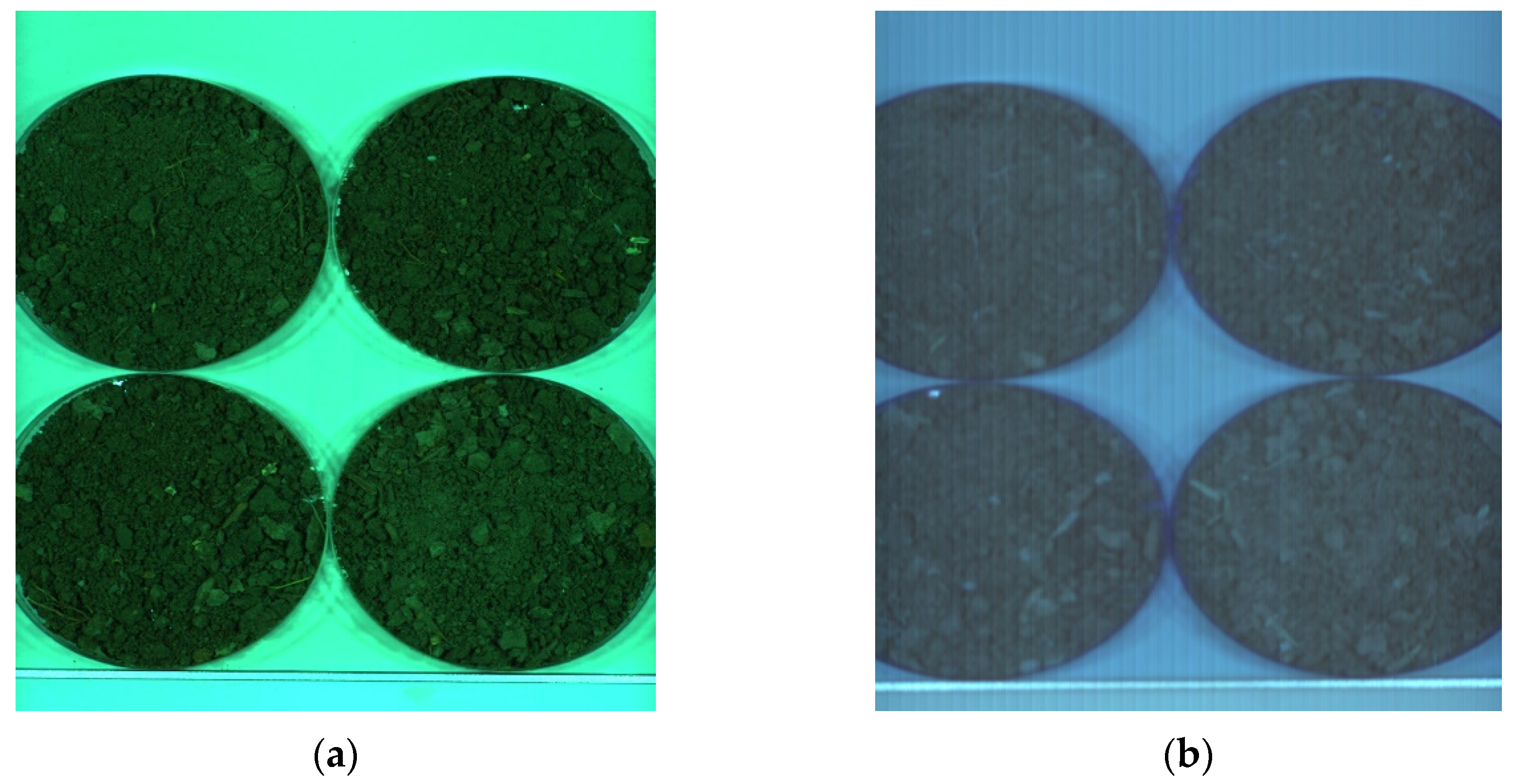
2.2. Field Data Collection and Processing

This study first investigated the relevant areas within the scope of Chair Hill and then collected cultivated soil samples at the experimental area in mid-to-late December 2019. The cultivated soil is often used for crops and tree planting, and its surface (0–10 cm depth) was chosen in the sample collecting area, which was located at the junction of sycamore and ginkgo trees, in an open location without covering branches above. Each sampling area was sized 15 × 15 cm, and a total of 9 samples were collected in one sampling operation. In total, 117 soil samples (excluding branches, roots, and other particulate impurities in the soil) were collected during the experiment, each with a net weight of 120 g. Among these samples, 52 sampling units were used for SMC detection, and 65 samples were used for reflectance spectra measurement of soil. The specific distribution of sampling points is shown in Figure 1b.

All spectral reflectance measurements were carried out in a laboratory at 15 °C. The experiment applied the GaiaSorter hyperspectral sorting system, which is equipped with SpectraSENS hyperspectral data acquisition software and two charge-coupled device (CCD) cameras. The collected samples were separately put into transparent petri dishes of 10 cm diameter, and placed in the instrument for data collection. The specific steps were as follows:

Step 1: To ensure the clarity of the image, the GaiaSorter hyperspectral sorting system was warmed up in advance, and parameters such as the height of the two cameras, the scanning forward speed, and the exposure time were set up as

Table 1. Parameters of GaiaSorter hyperspectral sorting system.

Number	Item	Parameter
1	Range of spectral scanning /nm	380–2500
2	Scanning forward speed /$\mathrm{cm}\left({\mathrm{s}}^{-1}\right)$	0.36
3	Height of camera (Camera 1/Camera 2) /cm	5/7

.

Step 2: Camera lens caps were removed and a standard whiteboard was used to calibrate the spectral reflectance by collecting an all-white image $D_w$ with a reflectivity of 1 under the above conditions. The lens caps were then replaced, and an all-black image $D_d$ was collected with a reflectivity of 0. According to Formula (1), the reflectance $\alpha$ at the region of interest (ROI) $s$ or band $i$ of the spectral image can be obtained after monochrome correction, which can overcome interference factors such as uneven light source distribution and image noise in some bands of the system and thus improve the SNR.

$$\alpha \left(si\right)=\frac{D_s\left(si\right)-D_d\left(si\right)}{D_w\left(si\right)-D_d\left(si\right)}$$

(1)

Step 3: Samples were placed on the stage and the "Start Scan" button in SpectraSENS was clicked. During data acquisition, the platform moved vertically toward the cameras to complete the process. Figure 2 shows images acquired by the GaiaSorter hyperspectral sorter system from camera 1 and camera 2. After gathering all of the samples’ data, ENVI software was used to obtain the ROI information from the hyperspectral images, and the average spectral value was selected as the value of the sample.

2.3. SMC Data Processing

The drying and time domain reflectometry (TDR) methods are commonly used as the SMC measurement technology. This research used the former to collect the SMC of each sampling unit. The procedure was as follows: (1) The surface soil was collected with a standard aluminum box, which was sealed immediately after collection; (2) an electronic balance with an accuracy of 0.01 g was used to weigh the box (denoted $m_1$). After continuously drying samples in an oven for 24 h at 105 °C, the boxes were taken out and measured again (denoted $m_2$). In this study, the SMC of the experiment was defined as the average water content of the soil units collected in the same batch under the same conditions, and the mass water content formula was applied to calculate its value:

$$\alpha (\%)=\frac{m_1-m_2}{m_1}\times 100\%$$

(2)

where $\alpha (\%)$ represents the soil moisture content (%); $m_1$ is the total mass of the soil sample and aluminum box before drying (g); $m_2$ is the total mass of the soil sample and aluminum box after drying (g).

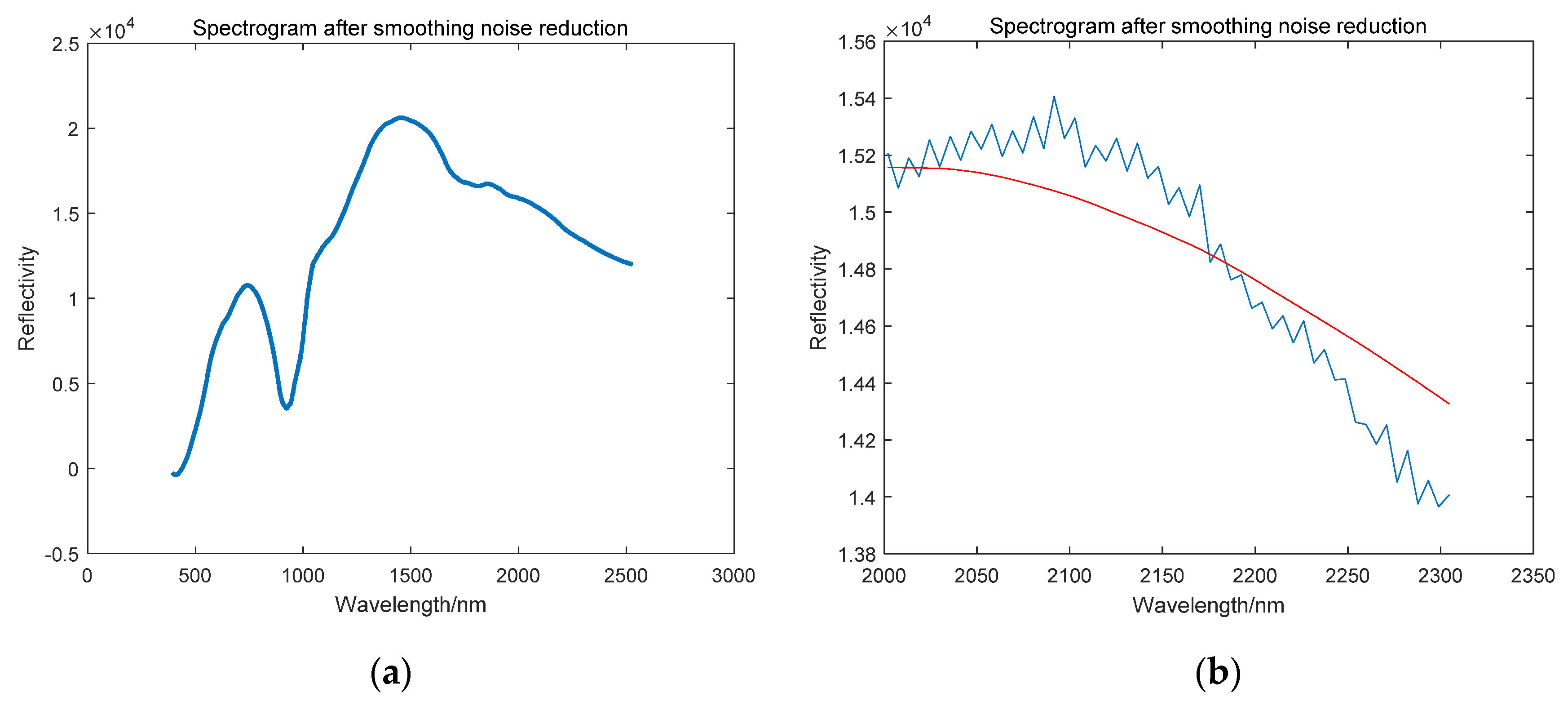
2.4. Hyperspectral Data Pretreatment

2.4.1. Wavelet Transform

The soil reflectance spectrum is subject to noise because of interference factors such as light conditions, air humidity, and spectrum acquisition instruments. In order to smooth the waveform and improve the SNR, this study used the wavelet transform algorithm for denoising.

Suppose $\phi \left(t\right)\in L^2\left(\mathit{R}\right)$, and if $\Phi \left(\omega \right)$, the Fourier transform of $\phi \left(t\right)$, satisfies the condition:

$${{\displaystyle \int }}_{\mathit{R}}{\left|\Phi \left(\omega \right)\right|}^2{\left|\omega \right|}^{-1}d\omega <+\infty$$

(3)

then $\phi \left(t\right)$ can be defied as a basic wavelet function.

A set of function sequences $\left\{{\phi }_{\beta ,\gamma }\left(t\right)\right\}$ can be obtained by expanding and translating $\phi \left(t\right)$:

$${\phi }_{\beta ,\gamma }\left(t\right)={\beta }^{-\frac{1}{2}}\phi \left(\frac{t-\gamma }{\beta }\right)$$

(4)

where $\beta >0,\gamma \in \mathit{R}$; $\beta$ is the scale factor and $\gamma$ is the translation factor.

Assuming that $\beta =2^{-j}$, $\gamma =k{2}^{-j}$, $j,k\in \mathrm{Z}$, and, as for any signal $f\left(t\right)\in L^2\left(\mathit{R}\right)$, its discrete wavelet function can be denoted:

$${\phi }_{2^{-j},k{2}^{-j}}\left(t\right)={\phi }_{j,k}\left(t\right)=2^{\frac{j}{2}}\phi \left(2^{j}t-k\right)dt$$

(5)

In this research, the spectral data was treated as a signal sequence of finite length. Therefore, its discrete wavelet transform can be described as:

$$W{T}_f\left(j,k\right)={\displaystyle \sum }_{n\in Z}f\left(n\right){\overline{\phi }}_{j,k}\left(n\right)$$

(6)

where $f\left(n\right)$ is the signal sequence; ${\phi }_{j,k}\left(n\right)$ is the basic wavelet function, and ${\overline{\phi }}_{j,k}\left(n\right)$ is the conjugate of ${\phi }_{j,k}\left(n\right)$.

2.4.2. Wavelet Denoising

When the signal $x\left(t\right)$ is contaminated by noise and becomes $s\left(t\right)$, the noise-containing signal model can be expressed as:

$$s\left(t\right)=x\left(t\right)+n\left(t\right)$$

(7)

where $n\left(t\right)$ is the Gaussian white noise signal, which is subject to the distribution $N\left(0,{\sigma }^2\right)$.

The wavelet coefficients of $s\left(t\right)$ can be determined as $w_{j,k}$ using a linear wavelet transform. Thresholding is key to wavelet denoising, and contains the selection of the threshold function and threshold estimation. The soft threshold function was performed in this experiment:

$$\widehat{w_{j,k}}=\{\begin{array}{cc}\hfill 0,& \left|w_{j,k}\right|<\tau \hfill \\ \hfill sig\left(w_{j,k}\right)\left(\left|w_{j,k}\right|-\tau \right),& \hfill \left|w_{j,k}\right|\ge \tau \end{array}$$

(8)

where $\tau$ is the threshold, which is defined as $\tau =\sqrt{2{\log }_{10}N}$, N is the length of the signal [23].

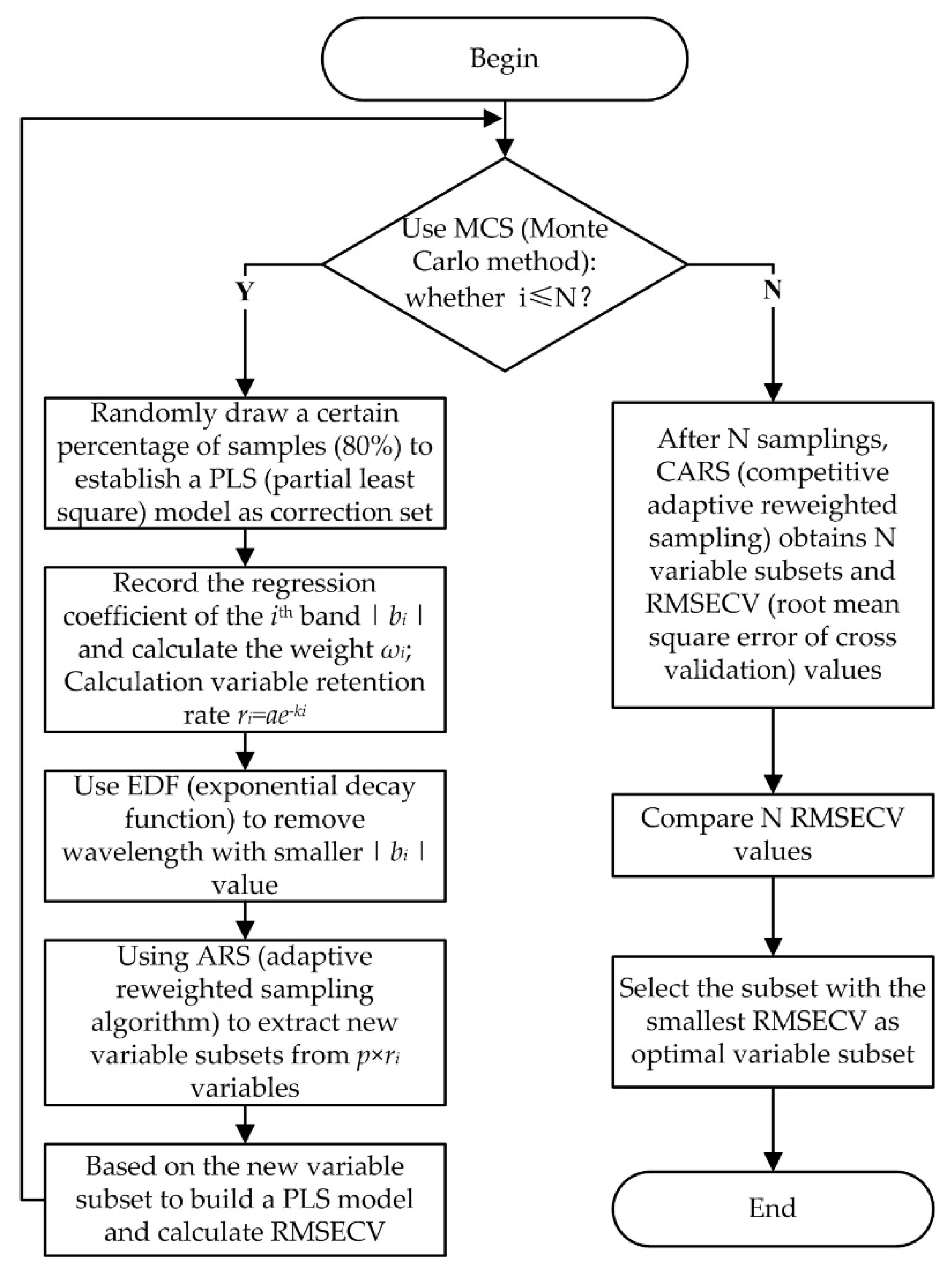
2.5. CARS-SPA Based Feature Wavelength Optimization

A wide range of bands, and large number of bands, were collected in this experiment. To select fewer characteristic wavelengths as the independent variables of the regression equation, the CARS-SPA algorithm was used in this study.

Competitive adaptive reweighted sampling (CARS) is an algorithm based on the rule of "survival of the fittest". In this study, it formed the basis of the regression coefficient calculated in a partial least squares (PLS) model, combined with the Monte Carlo sampling method to filter out the characteristic wavelength subset and the exponential decay function (EDF) to remove the wavelengths with smaller weight values [24]. Figure 3 demonstrates the processing procedure of the CARS algorithm.

The definition of the weight ${\omega }_i$ in Figure 3 is:

$${\omega }_i=\frac{\left|b_i\right|}{{{\displaystyle \sum }}_{i=1}^p\left|b_i\right|}$$

(9)

where $i=1,2,\dots ,p$, and p is the variable number. Generally, N = 50 is set in the Monte Carlo method [19].

The determining equations of a and k in the r_i formula in Figure 3 are as follows:

$$a={\left(\frac{p}{2}\right)}^{\frac{1}{N-1}}$$

(10)

$$k=\frac{\ln \frac{p}{2}}{N-1}$$

(11)

After using CARS to roughly screen some characteristic wavelengths, this study used the successive projections algorithm (SPA) to continuously find the optimal characteristic wavelength in the spectra as the independent variable of the inversion model. The SPA uses the multivariate linear regression (MLR) algorithm to select the optimal wavelength data, which are evaluated by obtaining and comparing the root mean square error of cross validation (RMSECV) values. The smaller the RMSECV, the better the achieved results [25]. The absolute values of the wavelengths’ regression coefficients contained in the dataset are rated, and the wavelengths with larger regression coefficients are selected to build the MLR model. After recording and assessing the RMSECV, the optimum wavelength and its number will be determined. The calculation process of the SPA is as follows:

Matrix xcal (N × M) is the training set used to build the model, $x_i$ is the $i^{th}$ column of the matrix, std is the position dataset of unselected column vectors after each screening (i.e., unselected band combination), and N is the number of samples.

Step 1: Select one of the wavelengths as the starter k[0], meanwhile set n = 1;

Step 2: Calculate the projection values of all of the wavelengths $x_i$ in the dataset std on the orthogonal space at $x_{k\left(n-1\right)}$:

$$P{x}_i=x_i-\left(x_i^T{x}_{k\left(n-1\right)}\right)x_{k\left(n-1\right)}{(x_{k\left(n-1\right)}^T{x}_{k\left(n-1\right)})}^{-1}$$

(12)

Step 3: Calculate the maximum projection value of wavelength k[n] and put it into std while letting n = n + 1:

$$k\left[n\right]=\arg \left(max\left|\right|P{x}_i\left|\right|\right),i\in std$$

(13)

Step 4: When n < N, return to Step 2;

Step 5: Evaluate the new set of selected variables through multiple linear regression, and ultimately obtain the preferred band combination {k[m]}, m = 1, 2, …, M−1.

SPA can reduce the redundancy of the original spectrum information and the number of variables that determine the linear regression models, thus ensuring the accuracy of the models while effectively reducing the fitting complexity and improving the simulation velocity. This feature can be used as a major advantage for establishing highly simplified inversion models [26].

2.6. Linear Regression Forecasting Model of Soil Moisture Content

2.6.1. Simple Linear Regression Model

If the independent variable of the simple linear regression model is x and the dependent variable is y, then the basic equation is:

$$y_i=a{x}_i+b+\epsilon$$

(14)

where a and b are undetermined parameters; i = 1, 2, ……, n (n represents the total number of experimental datapoints); $\epsilon$ represents a random parameter.

The least squares method can be used to obtain the simple linear regression model as:

$$\widehat{y}=\widehat{a}x+\widehat{b}$$

(15)

$$\widehat{a}=\overline{y}-\widehat{a}\overline{x}$$

(16)

$$\widehat{b}=\frac{{\sum }_{i=1}^n\left(x_i-\overline{x}\right)\left(y_i-\overline{y}\right)}{{\sum }_{i=1}^n{\left(x_i-\overline{x}\right)}^2}$$

(17)

where $\widehat{y}$ is the predicted value of y; $\widehat{a}$ is the predicted value of a; $\widehat{b}$ is the predicted value of b; $\overline{x}$ is the average of x; $\overline{y}$ is the average of y.

2.6.2. Multiple Linear Regression Model

The multiple linear regression (MLR) inversion model established in this study was a combination of characteristic wavelengths based on the selective data sets. The basic form of the MLR model is:

$$y_j={\beta }_1{x}_{1j}+{\beta }_2{x}_{2j}+\cdots +{\beta }_k{x}_{kj}+a+{\epsilon }_j$$

(18)

where the independent variables are $x_j$; the dependent variable is y; a and ${\beta }_j$ are undetermined parameters; j = 1, 2, ……, n (n represents the total number of experimental datapoints); ${\epsilon }_j$ represents random parameter [27].

In this research, the value of k was set as 2, and the MLR model was combined with independent variables selected from 7 characteristic wavelengths. The MLR models can achieve higher inversion accuracy by considering more factors in the equation than are considered by simple linear regression models. The optimal SMC inversion models are determined by the evaluation parameters.

2.7. Parameters of Model Evaluation

This research used the root mean square error (RMSE), coefficient of determination ($R^2$), and mean absolute error (MAE) to evaluate the accuracy of the inversion model. RMSE and MAE have inverse relationships with model performance, and a proportional relationship exists between $R^2$ ($R^2\in \left[0,1\right]$) and the performance of the model. The mathematical representations of these parameters can be expressed as follows:

(1)

Root mean square error

$$RMSE=\sqrt{\frac{{\sum }_{i=1}^n{({\widehat{y}}_i-y_i)}^2}{n}}$$

(19)

(2)

Coefficient of determination

$$R^2=\frac{{\sum }_{i=1}^n{\left({\widehat{y}}_i-\overline{y}\right)}^2}{{\sum }_{i=1}^n{\left(y_i-\overline{y}\right)}^2}$$

(20)

(3)

Mean absolute error

$$MAE=\frac{1}{n}{\displaystyle \sum }_{i=1}^n\left|\widehat{y_i}-y_i\right|$$

(21)

3. Results and Discussions

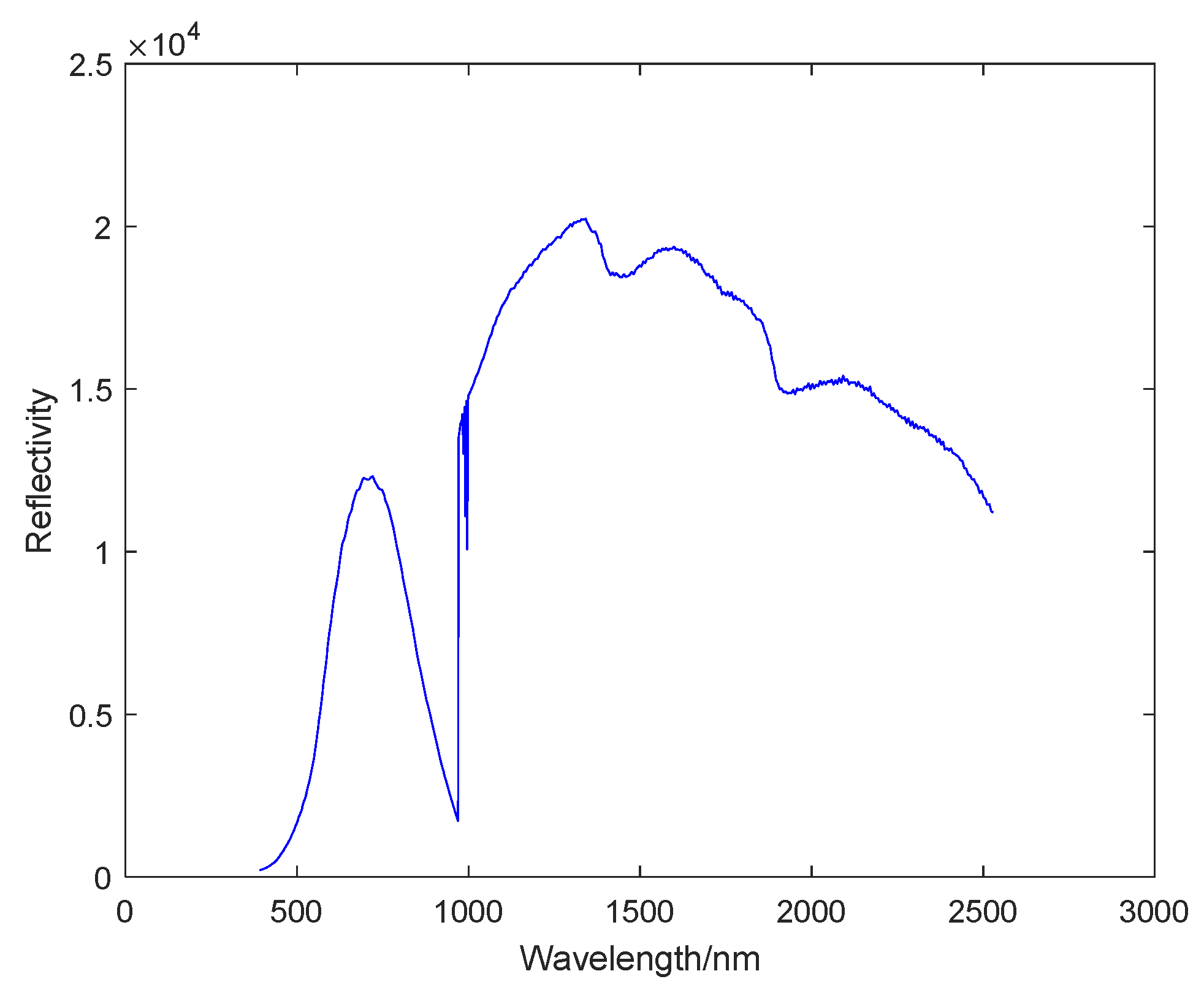
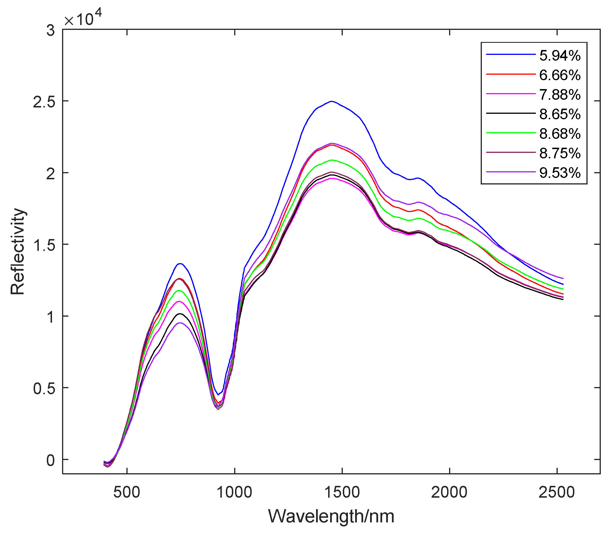
3.1. Results of SMC and Soil Spectral Data

In this paper, the drying method and GaiaSorter hyperspectral sorting system were respectively used to collect the SMC values and spectral data.

Table 2. Statistics of soil moisture content (SMC).

Soil Samples	Minimum of SMC	Maximum of SMC	Average of SMC	Variance	Coefficient of Variation
52	4.83%	9.92%	7.90%	0.013%	14.42%

presents the statistics of SMC measured in the experiment.

After collecting soil spectral reflectance data and SMC, this study used wavelet transform and wavelet denoising to improve the SNR of the spectrum. The spectral reflectance for each SMC was the average of the spectra data collected under the same sampling conditions. The spectrum was set as $s\left(t\right)$, which represents the discrete signal with noise [23]. Seven layers of "db4" decompositions were applied to the original basic wavelet function through MATLAB and the wavelet coefficients of each layer were used to reconstruct the spectrum. According to the Figure 4, the original waveform showed significant noises at 1000–1200 nm.

After using wavelet transform from layer 1 to 7, the spectrum was progressively smoother because of the removal of high-frequency signals. However, some sensitive bands of the spectrum were removed; for example, the peak between 380 and 1000 nm can still be seen in the layer 6 decomposition, but is invisible in layer 7. The training results indicate that a good smoothing effect was achieved in the 6-layer "db4" decomposition process, and the correlation coefficient with the original data was 0.912. Figure 5 shows the L6 full-spectrum smoothing diagram and its partially enlarged view in the 2002–2304 nm band.

Figure 6 shows part of the collected SMC and its corresponding reflectance spectrum. The following rules can be seen from Figure 6: (1) The spectral reflectance values tend to rise first and then decrease in the bands of 380–1000 nm and 1000–2530 nm, that is, there are reflection peaks in these two ranges. Furthermore, there is an absorption valley in the near-infrared band between 1000 and 1350 nm. (2) The span of 380–1000 nm conforms to the law that the spectral reflectance gradually decreases with the increase of SMC. However, in the 1000–2530 nm band, this law is not obvious. The spectra with large differences in SMC generally conform to the law that the spectrum decreases with increasing SMC.

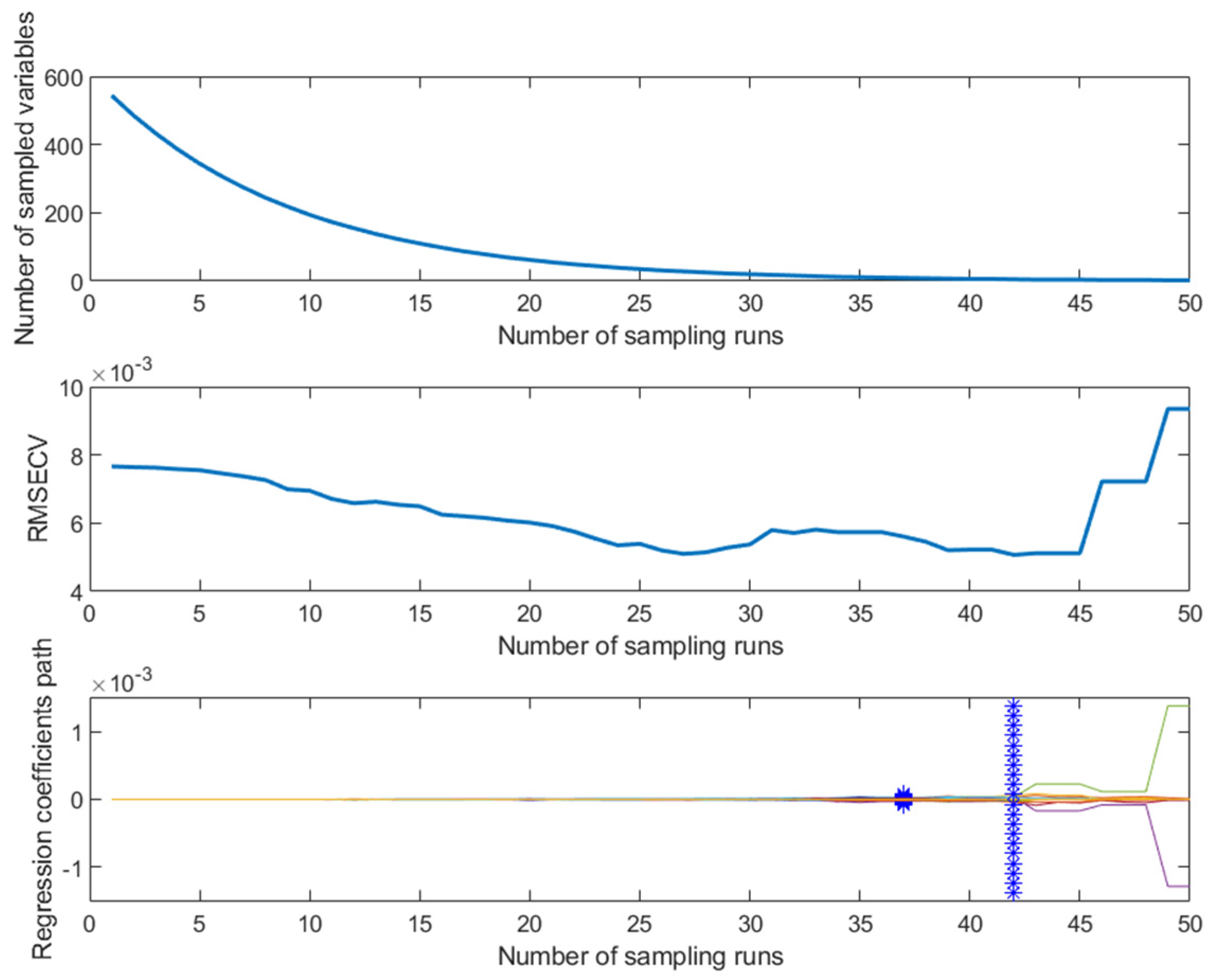
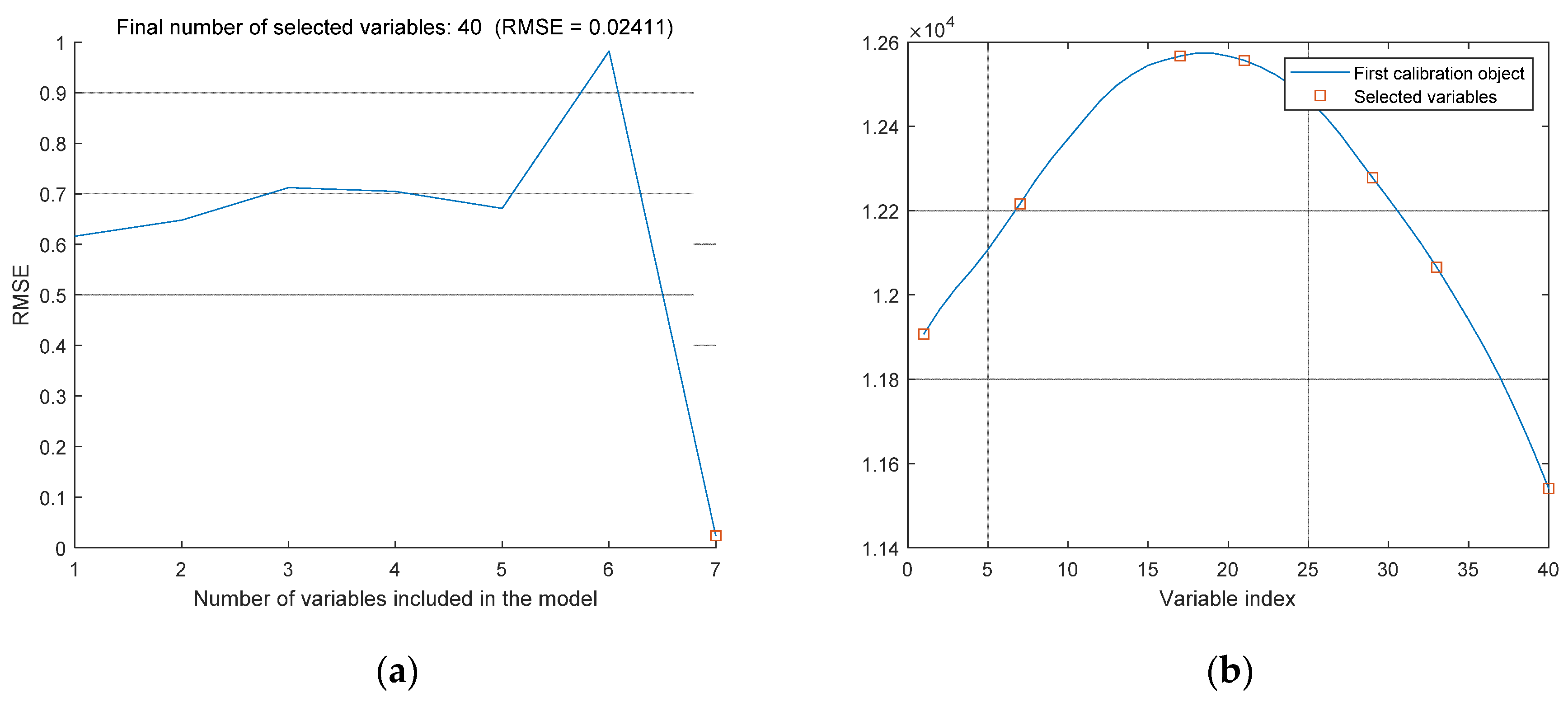
3.2. Processing Results of CARS-SPA Algorithm

This research used the CARS-PLS algorithm to perform the first round of screening for the pretreated soil spectrum’s full-spectral variables. Simultaneously, the data were processed separately by the CARS and the SPA to compare the accuracy of different algorithms.

CARS can be used to filter out unsuitable wavelengths in the band. This experiment set 50 as the number of Monte Carlo samples [24]. In the 1st to 15th iterations, the RMSECV value decreased. Thereafter, however, the RMSECV value started to rise slowly. Figure 7 represents the unprocessed spectral information using CARS to screen variables. It can be seen that the RMSECV value gradually decreased in the 1–32 iterations and, from the 33rd iteration, the RMSECV gradually increased. The minimum RMSECV at the 32nd iteration was 0.5431.

Table 3. Performance of models built by CARS-SPA algorithm.

Variable Selection Methods	Range of Band	Number of Variables	Number of Factors	RMSECV (Root Mean Square Error of Cross Validation)
CARS (competitive adaptive reweighted sampling)	380–2530 nm	544	124	0.523
SPA (successive projections algorithm)	380–2530 nm	544	10	0.477
CARS-SPA (competitive adaptive reweighted sampling combined with successive projections algorithm)	1273–1474 nm	32	7	0.413
CARS-SPA	695–796 nm	40	7	0.024

illustrates the comparison of selected wavelengths and RMSECV of CARS, SPA, and CARS-SPA algorithms. In Table 3, when using the CARS-SPA algorithm to process the spectral data, CARS was first used to filter the spectrum of the full band. After the characteristic wavelength dataset was obtained, SPA was then used to carry out a more detailed evaluation and finally obtain the optimal wavelengths.

As shown in Table 3, when the CARS and SPA algorithms were used independently to process the full band, the performance of the model constructed using the SPA algorithm was better than that constructed using CARS. Furthermore, the performance of the model using the CARS-SPA algorithm was significantly more accurate than the first two models, which is consistent with the conclusion of Cai et al. [19]. The result of this research also illustrates that the CARS-SPA algorithm has the least characteristic factors compared with the CARS and SPA algorithms. Therefore, using the CARS-SPA algorithm can not only reduce the complexity of the model, but also improves its accuracy. The CARS algorithm first optimized 124 characteristic wavelengths, of which 40 characteristic wavelengths were between 695 and 796 nm, and 32 characteristic wavelengths were between 1273 and 1474 nm. Figure 8 shows the result of further filtering characteristic wavelengths between 695 and 796 nm using the SPA algorithm. It can be observed from the diagram that seven characteristic wavelengths were finally obtained in this band, among which, the minimum RMSECV was at 778 nm, at which point the fitting effect of the model was optimal. Finally, the wavelengths of 695, 711, 736, 747, 767, 778, and 796 nm were selected as the inversion model factors.

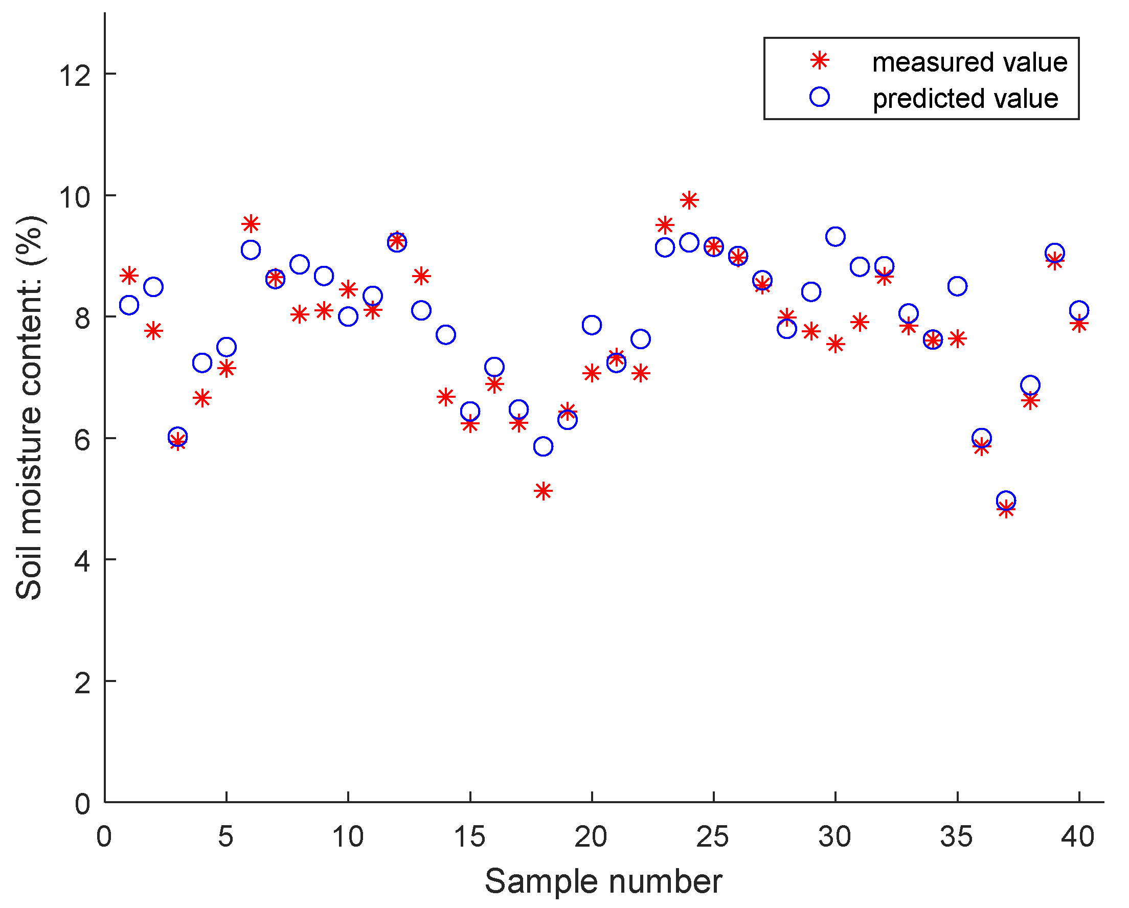
3.3. Results of Inversion Models

According to the selected results of CARS-SPA, the preferred wavelength was firstly subjected to simple linear regression analysis. Some of the simple linear inversion models and their accuracy results are listed in

Table 4. Simple linear inversion model and the accuracy.

Factor	Equation of Model	R2	RMSE (Root Mean Square Error)	MAE (Mean Absolute Error)
R736	Y = −6.682 $\times {10}^{-6}$ R736+0.1579	0.63	0.0084	0.0056
R747	Y = −6.717 $\times {10}^{-6}$ R747+0.1584	0.64	0.0084	0.0057
R778	Y = −7.092 $\times {10}^{-6}$ R778+0.16	0.65	0.0083	0.0056
R796	Y = −7.494 $\times {10}^{-6}$ R796+0.161	0.66	0.0082	0.0058

, which was constructed based on the factors of the seven characteristic wavelengths screened above. The R² values of the inversion models were between 0.63 and 0.66, the RMSE was between 0.0082 and 0.0084, and the MAE was 0.56–0.58%.

To improve the fitting degree of the model and the accuracy of the predicted value, this paper used the multivariate linear method for gradual regression to establish the inversion models [27].

Table 5. Multivariate linear inversion model and accuracy.

Number	Equation of Model	R2	RMSE
1	Y = −2.591 $\times {10}^{-5}$ R778+1.979 $\times {10}^{-5}$ R695+0.1567	0.74	0.0079
2	Y = −9.428 $\times {10}^{-5}$ R711+9.068 $\times {10}^{-5}$ R695+0.1518	0.75	0.0078
3	Y = −2.792 $\times {10}^{-5}$ R767+2.178 $\times {10}^{-5}$ R695+0.1555	0.74	0.0079
4	Y = −4.691 $\times {10}^{-5}$ R747+4.233 $\times {10}^{-5}$ R711+0.1519	0.73	0.0079
5	Y = −3.145 $\times {10}^{-5}$ R796+2.32 $\times {10}^{-5}$ R711+0.1592	0.73	0.0080

shows that the R² of the multiple linear regression equations increased to 0.75 compared with the simple linear regression equations. If Equation 3 in Table 5 was used to calculate the predicted SMC, the predicted R² value would be 0.822. Therefore, this study determined that multivariate linear inversion models composed of factors of 695, 711, 736, 747, 767, 778, and 796 nm could accurately deduce the soil moisture information.

Figure 9 shows the predicted SMC values obtained from the model based on the spectral data in the validation set.

$$\mathrm{Y}=-9.428\times {10}^{-5}{\mathrm{R}}_{711}+9.068\times {10}^{-5}{\mathrm{R}}_{695}+0.1518$$

(22)

The R² of the predicted SMC was 0.83, which proves that the inversion model can achieve a good prediction of the SMC.

4. Conclusions

In this study, based on the verified regular pattern in which the spectra of cultivated soil will decrease with increasing SMC, the SMC inversion models of cultivated soil were established using seven characteristic wavelength inversion factors: R₆₉₅, R₇₁₁, R₇₃₆, R₇₄₇, R₇₆₇, R₇₇₈, and R₇₉₆.

The results show that the inversion accuracy of the multiple linear inversion model is better than that of the simple linear regression model, with its predicted R² increasing to 0.82 and the RMSE decreasing from 0.0084 to 0.0078. The multivariate linear inversion model composed of R₆₉₅ and R₇₁₁ showed the best predictive ability, with a predicted R² of 0.83, and RMSE of 0.0078. The proposed models in this paper can be used as a reference for future research on the rapid prediction of large-scale SMC of cultivated soil through hyperspectral remote sensing images.

References

1. Corbari, C.; Sobrino, J.A.; Mancini, M.; Hidalgo, V. Land surface temperature representativeness in a heterogeneous area through a distributed energy-water balance model and remote sensing data. Hydrol. Earth Syst. Sci. 2010, 14, 2141–2151. [Google Scholar] [CrossRef] [Green Version]
2. Tian, L.; Zhao, L.; Wu, X.; Fang, H.; Zhao, Y.; Hu, G.; Yue, G.; Sheng, Y.; Wu, J.; Chen, J.; et al. Soil moisture and texture primarily control the soil nutrient stoichiometry across the tibetan grassland. Sci. Total Environ. 2018, 622–633, 192–202. [Google Scholar] [CrossRef]
3. Jun, X.U.; Jiang, J. Research on the estimation model of soil moisture content based on the characteristics of thermal infrared data. Asian J. Agric. Res. 2013, 5, 90–94. [Google Scholar]
4. Nsafon, B.E.K.; Lee, S.-C.; Huh, J.-S. Responses of Yield and Protein Composition of Wheat to Climate Change. Agriculture 2020, 10, 59. [Google Scholar] [CrossRef] [Green Version]
5. Bolten, J.D.; Crow, W.T.; Zhan, X.; Jackson, T.J.; Reynolds, C.A. Evaluating the utility of remotely sensed soil moisture retrievals for operational agricultural drought monitoring. IEEE J. Sel. Top Appl. Earth Obs. Remote Sens. 2010, 3, 57–66. [Google Scholar] [CrossRef] [Green Version]
6. Vereecken, H.; Schnepf, A.; Hopmans, J.W.; Javaux, M.; Young, I.M. Modeling soil processes: Key challenges and new perspectives. Vadose Zone J. 2016, 15, 1–57. [Google Scholar] [CrossRef] [Green Version]
7. Nagahage, E.A.A.D.; Nagahage, I.S.P.; Fujino, T. Calibration and Validation of a Low-Cost Capacitive Moisture Sensor to Integrate the Automated Soil Moisture Monitoring System. Agriculture 2019, 9, 141. [Google Scholar] [CrossRef] [Green Version]
8. Kerr, Y.H. Soil moisture from space: Where are we? Hydrogeol. J. 2007, 15, 117–120. [Google Scholar] [CrossRef]
9. Joshi, C.; Mohanty, B.P. Physical controls of near-surface soil moisture across varying spatial scales in an agricultural landscape during smex02. Water Resour. Res. 2010, 46, p.W12503.12501-W12503.12521. [Google Scholar] [CrossRef] [Green Version]
10. Sobrino, J.A.; Franch, B.; Mattar, C.; Jiménez-Muñoz, J.C.; Corbari, C. A method to estimate soil moisture from airborne hyperspectral scanner (ahs) and aster data: Application to sen2flex and sen3exp campaigns. Remote Sens. Environ. 2012, 117, 415–428. [Google Scholar] [CrossRef]
11. Stevanato, L.; Baroni, G.; Cohen, Y.; Fontana, C.L.; Gatto, S.; Lunardon, M.; Marinello, F.; Moretto, S.; Morselli, L. A Novel Cosmic-Ray Neutron Sensor for Soil Moisture Estimation over Large Areas. Agriculture 2019, 9, 202. [Google Scholar] [CrossRef] [Green Version]
12. Li, X.; Yu, T.; Wang, X.; Shang, X.; Chen, H. A grey relationship-based soil organic matter content inversion pattern. In Proceedings of the 2011 IEEE International Conference on Grey Systems and Intelligent Services, Nanjing, China, 15–18 September 2011; pp. 30–33. [Google Scholar] [CrossRef]
13. Yao, Y.; Wei, N.; Tang, P.; Li, Z.; Yu, Q.; Xu, X.; Chen, Y.; He, Y. Hyper-spectral characteristics and modeling of black soil moisture content. Trans. Chin. Soc. Agric. Eng. 2011, 27, 95–100. [Google Scholar]
14. Na, W.; Yao, Y.; Chen, Y. The advance of soil quality information monitoring by hyperspectral remote sensing. Chin. Agric. Sci. Bull. 2008, 24, 491–496. [Google Scholar]
15. Wang, C.; Feng, M.C.; Yang, W.D.; Guang-Xin, L.I.; Zhao, J.J.; Zhu, Z.H. Hyperspectrum monitoring of the som in plough layer in winter wheat filed. J. Shanxi Agric. Sci. 2014, 42, 869–873. [Google Scholar]
16. Zhang, J.H.; Jia, K.L. Spectral reflectance characteristics and modeling of typical takyr solonetzs water content. Chin. J. Appl. Ecol. 2015, 26, 884–890. [Google Scholar]
17. He, T.; Jing, W.; Lin, Z.; Ye, C. Spectral features of soil moisture. Acta Pedol. Sinica 2006, 43, 1027–1032. [Google Scholar]
18. Liu, W.D.; Baret, F.; Zhang, B.; Tong, Q.X.; Zheng, L.F. Using hyperspectral data to estimate soil surface moisture under experimental conditions. Int. J. Remote Sens. 2004, 8, 434–442. [Google Scholar]
19. Cai, L.H.; Ding, J.L. Prediction for soil water content based on variable preferred and extreme learning machine algorithm. Spectrosc. Spectr. Anal. 2018, 38, 2209–2214. [Google Scholar]
20. Wei, J.; Junlong, F.; Shuwen, W.; Runtao, W. Using cars-spa algorithm combined with hyperspectral to determine reducing sugars content in potatoes. J. Northeast Agric. Univ. 2016, 47, 88–95. [Google Scholar]
21. Peng, J.; Xiang, H.Y.; Wang, J.Q.; Liu, W.Y.; Chi, C.M.; Niu, J.L. Inversion models of soil water content using hyperspectral measurements in fields of the arid region farmland. Agric. Res. Arid Areas 2013, 31, 241–246. [Google Scholar]
22. Xiao-yan, Z.; Huan, L.; Li-ji, C.; Zhi-yuan, L. Critical spectral characteristics and moisture retrieval models of intertidal sediments. Adv. Mar. Sci. 2019, 37, 65–74. [Google Scholar]
23. Lu, J.; Ding, W. The feature extraction of plant electrical signal based on wavelet packet and neural network. In Proceedings of the International Conference on Automatic Control and Artificial Intelligence (ACAI 2012), Xiamen, China, 3–5 March 2012; pp. 2119–2122. [Google Scholar] [CrossRef]
24. Han, Y.; Chen, J.; Pan, T.; Liu, G. Determination of glycated hemoglobin using near-infrared spectroscopy combined with equidistant combination partial least squares. Chemometr. Intell. Lab. 2015, 145, 84–92. [Google Scholar] [CrossRef]
25. Hao, Q.; Zhou, J.; Zhou, L.; Kang, L.; Nan, T.; Yu, Y.; Guo, L. Prediction the contents of fructose, glucose, sucrose, fructo-oligosaccharides and iridoid glycosides in morinda officinalis radix using near-infrared spectroscopy. Spectrochim. Acta Part A Mol. Biomol. Spectrosc. 2020, 234, 118275. [Google Scholar] [CrossRef] [PubMed]
26. Ying, L.; Guo, Y.; Chang, L.; Wu, W.; Rao, P.; Fu, C.; Wang, S. Spa combined with swarm intelligence optimization algorithms for wavelength variable selection to rapidly discriminate the adulteration of apple juice. Food Anal. Methods 2016, 10, 1–7. [Google Scholar]
27. Jiang, G.; Grafton, M.; Pearson, D.; Bretherton, M.; Holmes, A. Integration of precision farming data and spatial statistical modelling to interpret field-scale maize productivity. Agriculture 2019, 9, 237. [Google Scholar] [CrossRef] [Green Version]
Figure 1. Location of the study area and distribution of sampling points: (a) location of the Chair Hill; (b) distribution of sampling points.
Agriculture 10 00292 g001
Figure 2. Images acquired by the GaiaSorter hyperspectral sorter system: (a) picture collected by Camera 1 (380–1100 nm); (b) picture collected by Camera 2 (900–2500 nm).
Agriculture 10 00292 g002
Figure 3. Flow chart of the CARS (competitive adaptive reweighted sampling) algorithm.
Agriculture 10 00292 g003
Figure 4. The original waveform of full-spectrum.
Agriculture 10 00292 g004
Figure 5. Results of wavelet transform and noise reduction: (a) L6 full-spectrum smoothing diagram; (b) smoothing effect picture (2002–2304 nm).
Agriculture 10 00292 g005
Figure 6. Soil reflectance spectrum of different SMC.
Agriculture 10 00292 g006
Figure 7. CARS algorithm processing result of the unprocessed full-band spectrum.
Agriculture 10 00292 g007
Figure 8. The characteristic wavelength selection results of the SPA algorithm at 695–796 nm in the CARS-SPA algorithm: (a) number of selected variables included in the model; (b) index of selected variables.
Agriculture 10 00292 g008
Figure 9. Comparison of predicted and actual values of SMC.
Agriculture 10 00292 g009