Mathematical Approach to Estimating the Main Epidemiological Parameters of African Swine Fever in Wild Boar

 , ,
, , 
 , and
, and
Abstract
1. Introduction
2. Materials and Methods
2.1. Sardinian Epidemiological Context
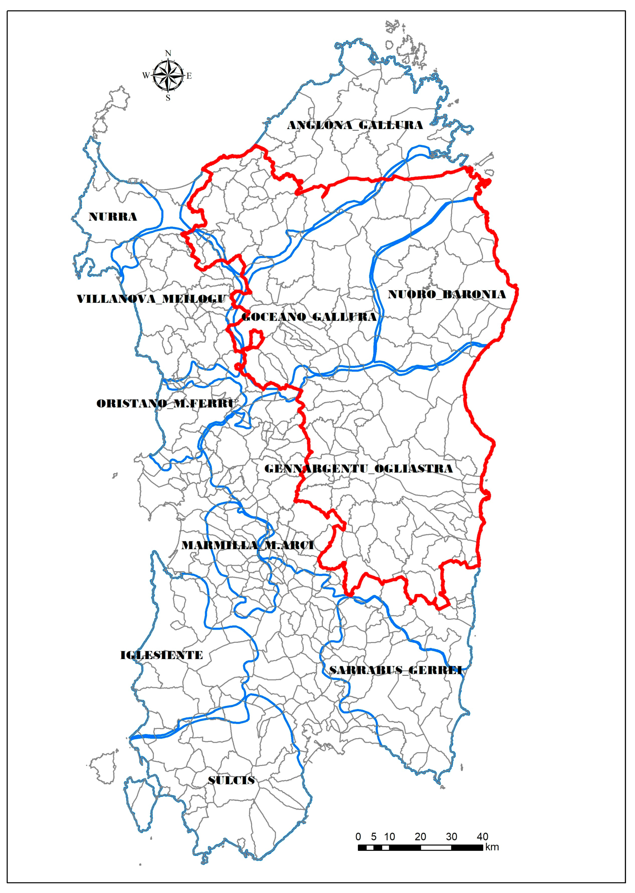
2.2. Wild Boar Management Unit of Anglona-Gallura
2.3. Data Collection
2.4. Estimates of the ASFV Force of Infection
2.4.1. Method 1: Estimating λ by Contact Rate
2.4.2. Method 2: Estimating λ Using a Catalytic Model
2.4.3. Method 3: Estimating λ Based on Proportion of Infected
2.5. Basic Reproduction Number (R0) Estimation
2.5.1. Method 1: Estimating R0 from the Doubling Time
2.5.2. Method 2: Estimating R0 from the Force of Infection (λ)
2.5.3. Method 3: Estimating R0 from the Proportion of Infected
2.5.4. Method 4: Estimating R0 from a Simple Susceptible-Exposed-Infectious-Recovered (SEIR) Model (Optimization Analysis)
2.6. Effective Reproduction Number (Re) Estimation
3. Results
4. Discussion
5. Conclusions
- (1)
- (2)
- The efficiency of passive surveillance proves that the absence of the virus (i.e., number of negative carcasses found with respect to the local wild boar population) is far from being known and standardized;
- (3)
- The absence of virus-positive animals among the hunted wild boar for a long time, as associated with serological data, provides valuable information for confirming that the disease is moving toward self-extinction; and
- (4)
- The seropositive and virus-negative animals that are still considered carriers despite their presence do not lead to any further virus detection, as confirmed by this study and in other similar epidemiological situation (e.g., in part of Estonia and Latvia). Notably, ASFV-specific antibodies in a wild boar population were found several years after the fading out of the virus [20,60,61,62,63].
Supplementary Materials
Author Contributions
Funding
Acknowledgments
Conflicts of Interest
References
- World Organization for Animal Health (OIE). Global Control of African Swine Fever, Resolution No. 33, 87 GS/FR; OIE Bulletine: Paris, France, 2019. [Google Scholar]
- Beltran-Alcrudo, D.; Falco, J.R.; Raizman, E.; Dietze, K. Transboundary spread of pig diseases: The role of international trade and travel. BMC Vet. Res. 2019, 15, 64. [Google Scholar] [CrossRef]
- Halasa, T.; Bøtner, A.; Mortensen, S.; Christensen, H.; Toft, N.; Boklund, A. Simulating the epidemiological and economic effects of an African swine fever epidemic in industrialized swine populations. Vet. Microbiol. 2016, 193, 7–16. [Google Scholar] [CrossRef]
- World Organization for Animal Health (OIE). Experts Meet in Early December to Prevent African Swine Fever. 2019. Available online: https://rr-americas.oie.int/wp-content/uploads/2019/12/eng_oie_press-release_1st-sge_asf_americas.pdf (accessed on 30 August 2020).
- Blome, S.; Gabriel, C.; Beer, M. Pathogenesis of African swine fever in domestic pigs and European wild boar. Virus Res. 2013, 173, 122–130. [Google Scholar] [CrossRef] [PubMed]
- Dixon, L.K.; Stahl, K.; Jori, F.; Vial, L.; Pfeiffer, D.U. African Swine Fever Epidemiology and Control. Annu. Rev. Anim. Biosci. 2019, 8, 221–246. [Google Scholar] [CrossRef]
- Costard, S.; Wieland, B.; de Glanville, W.; Jori, F.; Rowlands, R.; Vosloo, W.; Roger, F.; Pfeiffer, D.U.; Dixon, L.K. African swine fever: How can global spread be prevented? Philos. Trans. R. Soc. B 2009, 364, 2683–2696. [Google Scholar] [CrossRef] [PubMed]
- Chenais, E.; Depner, K.; Guberti, V.; Dietze, K.; Viltrop, A.; Ståhl, K. Epidemiological considerations on African swine fever in Europe 2014–2018. Porc. Health Manag. 2019, 5, 6. [Google Scholar] [CrossRef] [PubMed]
- Barongo, M.B.; Ståhl, K.; Bett, B.; Bishop, R.P.; Fèvre, E.M.; Aliro, T.; Okoth, E.; Masembe, C.; Knobel, D.; Ssematimba, A. Estimating the Basic Reproductive Number (R0) for African Swine Fever Virus (ASFV) Transmission between Pig Herds in Uganda. PLoS ONE 2015, 10, e0125842. [Google Scholar] [CrossRef] [PubMed]
- Mulumba-Mfumu, L.K.; Saegerman, C.; Dixon, L.K.; Madimba, K.C.; Kazadi, E.; Mukalakata, N.T.; Oura, C.A.; Chenais, E.; Masembe, C.; Ståhl, K.; et al. African swine fever: Update on Eastern, Central and Southern Africa. Transbound. Emerg. Dis. 2019, 66, 1462–1480. [Google Scholar] [CrossRef]
- Laddomada, A.; Rolesu, S.; Loi, F.; Cappai, S.; Oggiano, A.; Madrau, M.P.; Sanna, M.L.; Pilo, G.; Bandino, E.; Brundu, D.; et al. Surveillance and control of African swine fever in free- ranging pigs in Sardinia. Transbound. Emerg. Dis. 2019, 66, 1114–1119. [Google Scholar] [CrossRef] [PubMed]
- Commission Implementing Decision (EU) 2020/1211 of 20 August 2020 Amending the Annex to Implementing Decision 2014/709/EU Concerning Animal Health Control Measures Relating to African Swine Fever in Certain Member States (Notified under Document C(2020) 5802). Available online: https://eur-lex.europa.eu/legal-content/EN/TXT/PDF/?uri=CELEX:32020D1211&from=EN (accessed on 30 August 2020).
- Penrith, M.L.; Vosloo, W. Review of African swine fever: Transmission, spread and control. J. S. Afr. Vet. Assoc. 2009, 80, 58–62. [Google Scholar] [CrossRef]
- Doyle, S.; Blackie, B.; Ellis, A.; Komal, J.; Seppey, F.; Poulin, A.C.; McAlpine, R.; Ross, J. Canada Leverages Public–Private Partnerships to Keep African Swine Fever at Bay; OIE Bulletin, Panorama: Paris, France, 2019; p. 3. [Google Scholar]
- World Organization for Animal Health (OIE). Manual of Diagnostic Tests and Vaccines for Terrestrial Animals 2019. Chapter 3.8.1—African Swine Fever (Infection with African Swine Fever Virus); OIE: Paris, France, 2019. [Google Scholar]
- World Organization for Animal Health (OIE). Standard Operating Procedures on Suspension, Recovery or Withdrawal of Officially Recognised Disease Status and Withdrawal of the Endorsement of Official Control Programmes of Members; OIE: Paris, France, 2020; Available online: https://www.oie.int/fileadmin/Home/eng/Animal_Health_in_the_World/docs/pdf/SOP/EN_SOP_Susp_Recovery.pdf (accessed on 3 July 2020).
- World Organization for Animal Health (OIE). WAHIS Interface—Disease Timelines. 2020. Available online: https://www.oie.int/wahis_2/public/wahid.php/Diseaseinformation/Diseasetimelines (accessed on 30 August 2020).
- Schulz, K.; Staubach, C.; Blome, S.; Viltrop, A.; Nurmoja, I.; Conraths, F.J.; Sauter-Louis, C. Analysis of Estonian surveillance in wild boar suggests a decline in the incidence of African swine fever. Sci. Rep. 2019, 9, 8490. [Google Scholar] [CrossRef] [PubMed]
- Nurmoja, I.; Mõtus, K.; Kristian, M.; Niine, T.; Schulz, K.; Depner, K.; Viltrop, A. Epidemiological analysis of the 2015–2017 African swine fever outbreaks in Estonia. Prev. Vet. Med. 2018. [Google Scholar] [CrossRef] [PubMed]
- Oļševskis, E.; Schulz, K.; Staubach, C.; Seržants, M.; Lamberga, K.; Pūle, D.; Ozoliņš, J.; Conraths, F.J.; Sauter-Louis, C. African swine fever in Latvian wild boar—A step closer to elimination. Transbound. Emerg. Dis. 2020, 1–15. [Google Scholar] [CrossRef] [PubMed]
- Loi, F.; Cappai, S.; Coccollone, A.; Rolesu, S. Standardized Risk Analysis Approach Aimed to Evaluate the Last African swine fever Eradication Program Performance, in Sardinia. Front. Vet. Sci. 2019, 6, 299. [Google Scholar] [CrossRef]
- Nishiura, H.; Chowell, G. The Effective Reproduction Number as a Prelude to Statistical Estimation of Time-Dependent Epidemic Trends. In Mathematical and Statistical Estimation Approaches in Epidemiology; Springer: Dordrecht, The Netherlands, 2009; pp. 103–121. [Google Scholar] [CrossRef]
- De Jong, M.C.M. Mathematical modeling in veterinary epidemiology: Why model building is important. Prev. Vet. Med. 1995, 25, 183–193. [Google Scholar] [CrossRef]
- Diekmann, O.; Heesterbeek, J.A. Matematical Epidemiology of Infectious Disease, Model Building, Analysis and Interpretation; John Wiley & Sons Ltd.: Hoboken, NJ, USA, 2000; pp. 4–29. [Google Scholar]
- Keeling, M.J.; Danon, L. Mathematical modelling of infectious diseases. Br. Med. Bull. 2009, 92, 33–42. [Google Scholar] [CrossRef]
- Vynnycky, E.; White, R.G. Introduction to Infectious Disease Modelling; Oxford University Press: Oxford, UK, 2010. [Google Scholar]
- Guinat, C.; Porphyre, T.; Gogin, A.; Dixon, L.; Pfeiffer, D.U.; Gubbins, S. Inferring within-herd transmission parameters for African swine fever virus using mortality data from outbreaks in the Russian Federation. Transbound. Emerg. Dis. 2018, 65, e264–e271. [Google Scholar] [CrossRef]
- Byamukama, M.; Tumwiine, J. Modeling and Stability Analysis of the African Swine Fever Epidemic Model. IOSR J. Math. (IOSR-JM) 2019, 15, 44–65. [Google Scholar]
- Marcon, A.; Linden, A.; Satran, P.; Gervasi, V.; Licoppe, A.; Guberti, V. R0 Estimation for the African Swine Fever Epidemicsin Wild Boar of Czech Republic and Belgium. Vet. Sci. 2020, 7, 2. [Google Scholar] [CrossRef]
- Cappai, S.; Rolesu, S.; Coccollone, A.; Laddomada, A.; Loi, F. Evaluation of biological and socio-economic factors related to persistence of African swine fever in Sardinia. Prev. Vet. Med. 2018, 152, 1–11. [Google Scholar] [CrossRef]
- Bosch, J.; Barasona, J.A.; Cadenas-Fernandez, E.; Jurado, C.; Pintore, A.; Denurra, D.; Cherchi, M.; Vicente, J.; Sanchez-Vizcaıno, J.M. Retrospective spatial analysis for African swine fever in endemic areas to assess interactions between susceptible host populations. PLoS ONE 2020, 15, e0233473. [Google Scholar] [CrossRef] [PubMed]
- FAO. African swine fever in the Russian Federation: Risk factors for Europe and beyond. In EMPRES WATCH; FAO: Rome, Italy, 2013; Volume 28. [Google Scholar]
- Boklund, A.; Cay, B.; Depner, K.; Foldi, Z.; Guberti, V.; Masilius, M.; Miteva, A.; More, S.; Olsevskis, E.; European Food Safety Authority (EFSA); et al. Scientific report on the epidemiological analyses of African swine fever in the European Union (November 2017 until November 2018). EFSA J. 2018, 16, e05494. [Google Scholar] [PubMed]
- Apollonio, M.; Luccarini, S.; Cossu, A.; Chirichella, R. Aggiornamento Della Carta Delle Vocazioni Faunistiche Della Sardegna. 2012. Available online: http://www.sardegnaambiente.it/documenti/18_269_20121204134127.pdf (accessed on 30 August 2020).
- King, D.P.; Reid, S.M.; Hutchings, G.H.; Grierson, S.S.; Wilkinson, P.J.; Dixon, L.K.; Bastos, A.D.; Drew, T.W. Development of a TaqMan® PCR assay with internal amplification control for the detection of African swine fever virus. J. Virol. Methods 2003, 107, 53–61. [Google Scholar] [CrossRef]
- Anderson, R.M.; May, R.M. Infectious Diseases of Humans: Dynamics and Control, 2nd ed.; Oxford University Press: Oxford, UK, 1991; Chapter 6. [Google Scholar]
- Griffiths, D.A. A catalytic model for infection for measles. Appl. Stat. 1974, 23, 330–339. [Google Scholar] [CrossRef]
- Munch, H. Catalytic Model in Epidemiology; Harvard University Press: Cambridge, MA, USA, 1959. [Google Scholar]
- Briedermann, L. Schwarzwild, 2nd ed.; VEB Deutscher Landwirtschaftsverlag: Leinen, Germany, 1990. [Google Scholar]
- Bieber, C.; Ruf, T. Population dynamics in wild boar Sus scrofa: Ecology, elasticity of growth rate and implications for the management of pulsed resource consumers. J. Appl. Ecol. 2005, 42, 1203–1213. [Google Scholar] [CrossRef]
- Bailey, N.T.J. The Mathematical Theory of Infectious Diseases and Its Applications, 2nd ed.; Hafner: New York, NY, USA, 1975. [Google Scholar]
- Farrington, C.P. Modelling force of infection for measles, mumps and rubella. Stat. Med. 1990, 9, 953–967. [Google Scholar] [CrossRef]
- Cutts, F.T.; Abebe, A.; Messele, T.; Dejene, A. Sero-epidemiology of rubella in the urban population of Addis Abeba, Ethiopia. Epidemiol. Infect. 2000, 124, 467–479. [Google Scholar] [CrossRef]
- Remme, J.; Mandara, M.P.; Leewenberg, J. The force of measles infection in Africa. Int. J. Epidemiol. 1984, 13, 332–339. [Google Scholar] [CrossRef]
- Beker, N. Analysis of Infectious Disease Data; Chapman and Hall: London, UK, 1989. [Google Scholar]
- Guinat, C.; Reis, A.L.; Netherton, C.L.; Goatley, L.; Pfeiffer, D.U.; Dixon, L. Dynamics of African swine fever virus shedding and excretion in domestic pigs infected by intramuscular inoculation and contact transmission. Vet. Res. 2014, 45, 93. [Google Scholar] [CrossRef]
- Blome, S.; Gabriel, C.; Dietze, K.; Breithaupt, A.; Beer, M. High virulence of African swine fever virus caucasus isolate in European wild boars of all ages. Emerg. Infect. Dis. 2012, 18, 708. [Google Scholar] [CrossRef]
- Gabriel, C.; Blome, S.; Malogolovkin, A.; Parilov, S.; Kolbasov, D.; Teifke, J.P.; Beer, M. Characterization of African swine fever virus Caucasus isolate in European wild boars. Emerg. Infect. Dis 2011, 17, 2342. [Google Scholar] [CrossRef] [PubMed]
- Costard, S.; Mur, L.; Lubroth, J.; Sanchez-Vizcaino, J.M.; Pfeiffer, D.U. Epidemiology of African swine fever virus. Virus Res. 2013, 173, 191–197. [Google Scholar] [CrossRef] [PubMed]
- Efron, B.; Tibshirani, R. Bootstrap methods for standard errors, confidence intervals, and other measures of statistical accuracy. Stat. Sci. 1986, 1, 54–75. [Google Scholar] [CrossRef]
- Favier, C.; Dégallier, N.; Rosa-Freitas, M.G.; Boulanger, J.P.; Costa Lima, J.R.; Luitgards-Moura, J.F.; Menkes, C.E.; Mondet, B.; Oliveira, C.; Weimann, E.T.S.; et al. Early determination of the reproduction number for vector-borne diseases: The case of dengue in Brazil. Trop. Med. Int. Health 2006, 11, 332–340. [Google Scholar] [CrossRef] [PubMed]
- Saltelli, A.; Ratto, M.; Andres, T.; Campolongo, F.; Cariboni, J.; Gatelli, D.; Saisana, M.; Tarantola, S. Global Sensitivity Analysis: The Primer; John Wiley & Sons: Chichester, UK, 2008. [Google Scholar]
- Diekmann, O.; Heesterbeek, J.A.; Metz, J.A. On the definition and the computation of the basic reproduction ratio R0 in models for infectious diseases in heterogeneous populations. J. Math. Biol. 1990, 28, 365–382. [Google Scholar] [CrossRef]
- Bettencourt, L.M.A.; Ribeiro, R.M. Real Time Bayesian Estimation of the Epidemic Potential of Emerging Infectious Diseases. PLoS ONE 2008, 3, e2185. [Google Scholar] [CrossRef]
- Chowell, G.; Nishiura, H.; Bettencourt, L.M. Comparative estimation of the reproduction number for pandemic influenza from daily case notification data. J. R. Soc. Interface 2007, 4, 155–166. [Google Scholar] [CrossRef]
- Clancy, D.; O’Neil, P.D. Bayesian estimation of the basic reproduction number in stochastic epidemic models. Bayesian Anal. 2008, 3, 737–758. [Google Scholar] [CrossRef]
- Schulz, K.; Conraths, F.J.; Blome, S.; Staubach, C.; Sauter-Louis, C. African swine fever: Fast and Furious or Slow and Steady? Viruses 2019, 11, 866. [Google Scholar] [CrossRef]
- Arias, M.; Sanchez-Vizcaino, J.M. African swine fever eradication: The Spanish model. In Trends in Emerging Viral Infections of Swine, 1st ed.; Morilla, A.K.J., Zimmerman, J., Eds.; Iowa State University Press: Ames, IA, USA, 2002; pp. 133–139. [Google Scholar]
- Guinat, C.; Gubbins, S.; Vergne, T.; Gonzales, J.T.; Dixon, L.; Pfeiffer, D.U. Experimental pig-to-pig transmission dynamics for African swine fever virus, Georgia 2007/1 strain. Epidemiol. Infect. 2016, 144, 25–34. [Google Scholar] [CrossRef]
- Penrith, M.L.; Thomson, G.R.; Bastos, A.D.S.; Phiri, O.C.; Lubisi, B.A.; Du Plessis, E.C.; Macome, F.; Pinto, F.; Botha, B.; Esterhuysen, J. An investigation into natural resistance to African swine fever in domestic pigs from an endemic area in southern Africa. Rev. Sci. Technol. 2004, 23, 965–977. [Google Scholar] [CrossRef] [PubMed]
- Pujols-Romeu, J.; Badiola-Saiz, J.I.; Perez de Rozas, A.M.; Rosell-Bellsola, R.; Carreras-Mauri, J. Papel quetienen los cerdos portadores en el mantenimiento ytransmisión del virus de la PPA. I. Estudio epizootiológico. Med. Vet. 1991, 8, 481–486, 488–489. [Google Scholar]
- Eblé, P.L.; Hagenaars, T.J.; Weesendorp, E.; Quak, S.; Moonen-Leusen, H.W.; Loeffen, W.L.A. Transmission of African Swine Fever Virus via carrier (survivor) pigs does occur. Vet. Microbiol. 2019, 273, 108345. [Google Scholar] [CrossRef] [PubMed]
- Stahl, K.; Sternberg-Lewerin, S.; Blome, S.; Viltrop, A.; Penrith, M.L.; Chenais, E. Lack of evidence for long term carriers of African swine fever virus—A systematic review. Virus Res. 2019, 272, 197725. [Google Scholar] [CrossRef] [PubMed]
- Miteva, A.; Papanikolaou, A.; Gogin, A.; Boklund, A.; Bøtner, A.; Linden, A.; Viltrop, A.; Schmidt, C.G.; Ivanciu, C.; European Food Safety Authority (EFSA); et al. Scientific report on the epidemiological analyses of African swine fever in the European Union (November 2018 to October 2019). EFSA J. 2020, 18, e05996. [Google Scholar]
- Cannon, R.M.; Roe, R.T. Livestock Disease Surveys: A Field Manual for Veterinarians; Australian Government Publishing Service: Canberra, Australia, 1982. [Google Scholar]
- Gervasi, V.; Marcon, A.; Bellini, S.; Guberti, V. Evaluation of the Efficiency of Active and Passive Surveillance in the Detection of African swine fever in Wild Boar. Vet. Sci. 2019, 7, 5. [Google Scholar] [CrossRef]


| Hunting Season | Wild Boar Age Classes | Wild Boar Virologically 1 Tested | Virus Prevalence | Wild Boar Serologically 2 Tested | Seroprevalence 3 |
|---|---|---|---|---|---|
| n (%) | (95% CI) | n (%) | (95% CI) | ||
| 2011–2012 | Young | 40 (33.6) | 0 (0–0) | 272 (28.1) | 0 (0–0) |
| Subadult | 47 (39.5) | 0 (0–0) | 277 (28.6) | 0 (0–0) | |
| Adult | 32 (26.9) | 6.4 (0.1–16.2) | 418 (43.3) | 0 (0–0) | |
| Total | 119 | 0.8 (0.2–4.6) | 967 | 0 (0–0) | |
| 2012–2013 | Young | 21 (17.2) | 0 (0–0) | 131 (19.5) | 0.8 (0.0–4.2) |
| Subadult | 34 (27.9) | 0 (0–0) | 171 (25.5) | 0.6 (0.0–3.2) | |
| Adult | 67 (54.9) | 1.5 (0.0–8.0) | 369 (55.0) | 0.5 (0.1–1.9) | |
| Total | 122 | 0.8 (0.0–4.5) | 671 | 0.6 (0.2–1.5) | |
| 2013–2014 | Young | 33 (6.8) | 0 (0–0) | 55 (4.5) | 5.5 (1.1–15.1) |
| Subadult | 191 (39.2) | 3.1 (1.2–6.7) | 368 (30.3) | 1.4 (0.4–3.1) | |
| Adult | 263 (54.0) | 4.2 (2.1–7.3) | 792 (65.2) | 0.8 (0.3–1.6) | |
| Total | 487 | 3.5 (2.0–5.5) | 1215 | 1.1 (0.6–1.9) | |
| 2014–2015 | Young | 33 (10.1) | 0 (0–0) | 80 (5.3) | 0 (0–0) |
| Subadult | 98 (29.9) | 0 (0–0) | 410 (27.3) | 0.5 (0.1–1.7) | |
| Adult | 197 (60.0) | 1.5 (0.3–4.4) | 1014 (67.4) | 3.5 (2.0–4.2) | |
| Total | 328 | 0.9 (0.2–2.6) | 1504 | 2.1 (1.4–3.0) | |
| 2015–2016 | Young | 53 (7.8) | 0 (0–0) | 95 (5.8) | 1.1 (0.0–5.7) |
| Subadult | 182 (27.0) | 0 (0–0) | 420 (25.4) | 0.2 (0.0–1.3) | |
| Adult | 440 (65.2) | 0.7 (0.1–2.0) | 1137 (68.8) | 2.9 (2.0–4.0) | |
| Total | 675 | 0.4 (0.0–1.3) | 1652 | 2.1 (1.5–2.9) | |
| 2016–2017 | Young | 64 (7.1) | 0 (0–0) | 117 (4.9) | 0 (0–0) |
| Subadult | 244 (27.1) | 0 (0–0) | 657 (27.7) | 0.9 (0.3–2.0) | |
| Adult | 591 (65.8) | 0 (0–0) | 1600 (67.4) | 1.4 )0.9–2.1) | |
| Total | 899 | 0 (0, 0–0) | 2374 | 1.2 (0.8–1.7) | |
| 2017–2018 | Young | 71 (6.1) | 0 (0–0) | 132 (5.9) | 0 (0–0) |
| Subadult | 364 (31.3) | 0 (0–0) | 679 (30.6) | 0.6 (0.2–1.5) | |
| Adult | 729 (62.6) | 0 (0–0) | 1408 (63.5) | 0.6 (0.2–1.1) | |
| Total | 1164 | 0 (0, 0–0) | 2219 | 0.5 (0.3–0.9) | |
| 2018–2019 | Young | 78 (6.1) | 0 (0–0) | 97 (4.2) | 0 (0–0) |
| Subadult | 290 (22.8) | 0 (0–0) | 531 (22.7) | 0 (0–0) | |
| Adult | 901 (71.1) | 0 (0–0) | 1709 (73.1) | 0.5 (0.2–0.9) | |
| Total | 1269 | 0 (0, 0–0) | 2337 | 0.3 (0.1–0.7) | |
| 2019–2020 | Young | 53 (4.0) | 0 (0–0) | 92 (3.9) | 0 (0–0) |
| Subadult | 339 (25.8) | 0 (0–0) | 599 (25.3) | 0.2 (0.0–0.9) | |
| Adult | 921 (70.2) | 0 (0–0) | 1674 (70.8) | 0.2 (0.1–0.6) | |
| Total | 1313 | 0 (0, 0–0) | 2365 | 0.2 (0.1–0.5) |
| Variable | N | Mean | SEM | 95% CI of Mean | Width of the CI |
|---|---|---|---|---|---|
| Week 1a | 23 | 39.874 | 0.859 | 38.189–41.558 | 3.368 |
| Week 1b | 21 | 8.056 | 0.350 | 7.369–8.742 | 1.373 |
| Week 2a | 22 | 42.073 | 0.943 | 40.223–43.922 | 3.699 |
| Week 2b | 24 | 10.632 | 0.448 | 9.753–11.511 | 1.758 |
| Week 3a | 21 | 40.000 | 0.878 | 38.278–41.722 | 3.444 |
| Week 3b | 22 | 9.476 | 0.391 | 8.708–10.243 | 1.535 |
| Week 4a | 24 | 38.000 | 0.973 | 36.092–39.908 | 3.816 |
| Week 4b | 22 | 11.000 | 0.471 | 10.076–11.924 | 1.848 |
| Parameter | Definition | Method | Estimate | 95% CI |
|---|---|---|---|---|
| λ | Force of infection (daily) | Based on contact rate β | 0.0056 | 0.0016–0.0092 |
| Catalytic model | 0.0024 | 0.0013–0.0035 | ||
| Based on average age at infection A | 0.0012 | 0.0004–0.0021 | ||
| A | Average age at infection (monthly) | Life expectancy | 28.5 | 28.1–29.9 |
| s | Proportion of susceptible/receptive population | Serology by age | 0.952 | 0.937–0.991 |
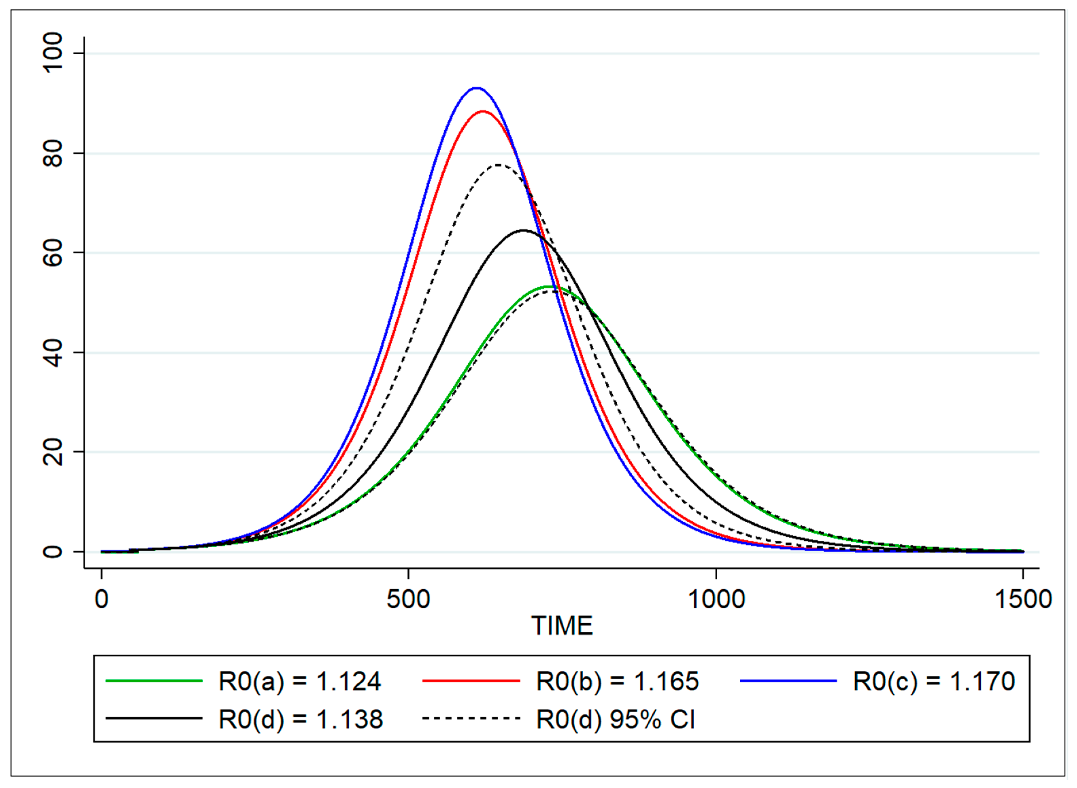
| R0 | Basic reproduction number | Doubling time | 1.124 | 1.103–1.145 |
| Based on force of infection λ | 1.165 | 1.027–1.301 | ||
| Proportion of infected | 1.170 | 1.009–1.332 | ||
| SEIR model (optimization) | 1.139 | 1.123–1.153 | ||
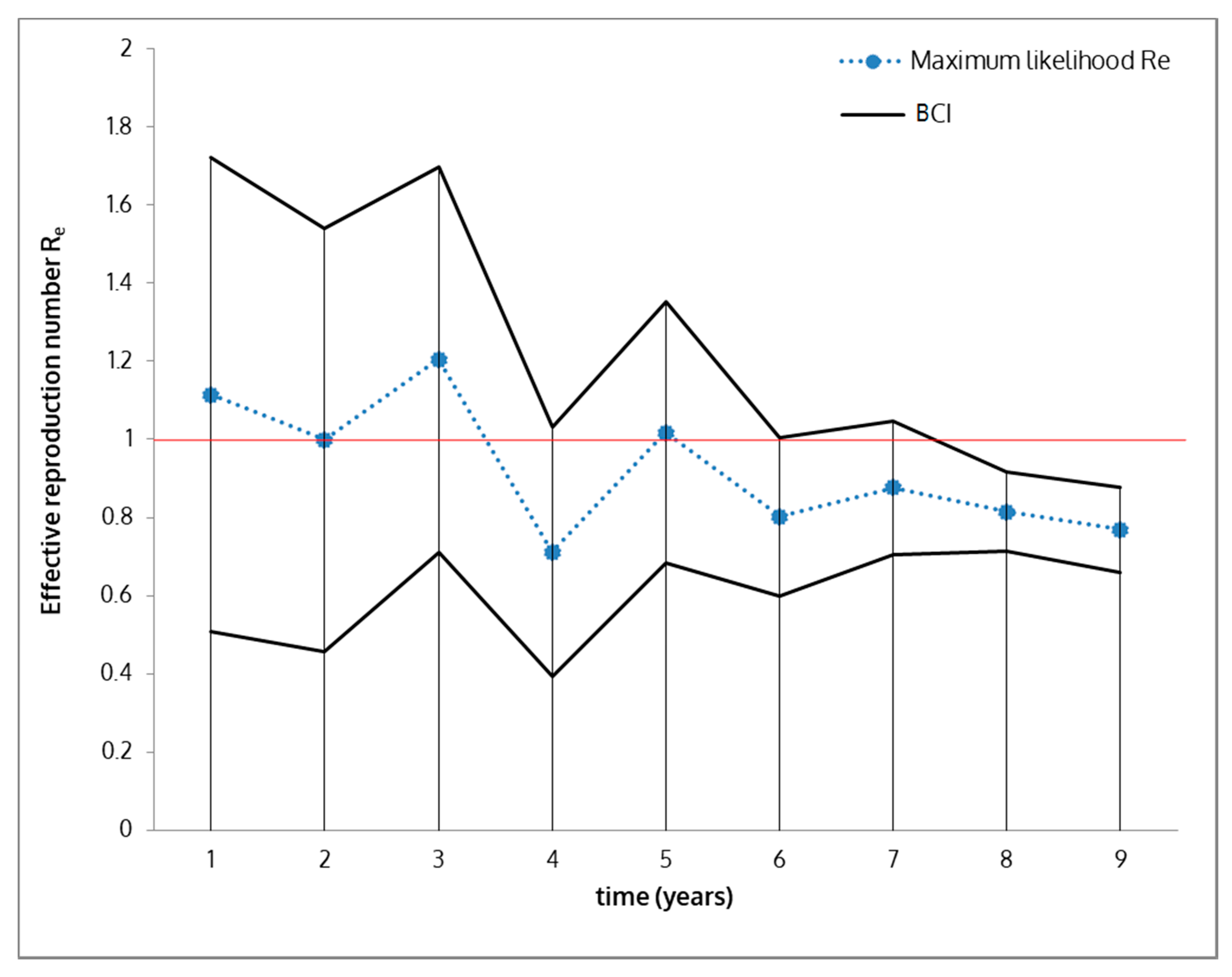
| Re | Effective reproduction number | Average value based on basic reproduction number R0 | 0.802 | 0.612–0.992 |
| Bayesian SEIR model (optimization) (BCI) | 0.923 | 0.812–1.033 | ||
| f | Infection rate | 1/average pre-infectious period [46,47,48] | 0.28 | – |
| r | Recovery rate | 1/infectious period [46,47,48] | 0.15 | – |
© 2020 by the authors. Licensee MDPI, Basel, Switzerland. This article is an open access article distributed under the terms and conditions of the Creative Commons Attribution (CC BY) license (http://creativecommons.org/licenses/by/4.0/).
Share and Cite
Loi, F.; Cappai, S.; Laddomada, A.; Feliziani, F.; Oggiano, A.; Franzoni, G.; Rolesu, S.; Guberti, V. Mathematical Approach to Estimating the Main Epidemiological Parameters of African Swine Fever in Wild Boar. Vaccines 2020, 8, 521. https://doi.org/10.3390/vaccines8030521
Loi F, Cappai S, Laddomada A, Feliziani F, Oggiano A, Franzoni G, Rolesu S, Guberti V. Mathematical Approach to Estimating the Main Epidemiological Parameters of African Swine Fever in Wild Boar. Vaccines. 2020; 8(3):521. https://doi.org/10.3390/vaccines8030521
Chicago/Turabian StyleLoi, Federica, Stefano Cappai, Alberto Laddomada, Francesco Feliziani, Annalisa Oggiano, Giulia Franzoni, Sandro Rolesu, and Vittorio Guberti. 2020. "Mathematical Approach to Estimating the Main Epidemiological Parameters of African Swine Fever in Wild Boar" Vaccines 8, no. 3: 521. https://doi.org/10.3390/vaccines8030521
APA StyleLoi, F., Cappai, S., Laddomada, A., Feliziani, F., Oggiano, A., Franzoni, G., Rolesu, S., & Guberti, V. (2020). Mathematical Approach to Estimating the Main Epidemiological Parameters of African Swine Fever in Wild Boar. Vaccines, 8(3), 521. https://doi.org/10.3390/vaccines8030521