Analysis of a Fractional-Order COVID-19 Epidemic Model with Lockdown

Abstract

The outbreak of the coronavirus disease (COVID-19) has caused a lot of disruptions around the world. In an attempt to control the spread of the disease among the population, several measures such as lockdown, and mask mandates, amongst others, were implemented by many governments in their countries. To understand the effectiveness of these measures in controlling the disease, several mathematical models have been proposed in the literature. In this paper, we study a mathematical model of the coronavirus disease with lockdown by employing the Caputo fractional-order derivative. We establish the existence and uniqueness of the solution to the model. We also study the local and global stability of the disease-free equilibrium and endemic equilibrium solutions. By using the residual power series method, we obtain a fractional power series approximation of the analytic solution. Finally, to show the accuracy of the theoretical results, we provide some numerical and graphical results.

1. Introduction and Preliminaries

The study of mathematical models of infectious diseases has attracted the attention of many researchers since they provide a better understanding of their evaluations, existence, stability, and control [1,2,3,4,5,6]. Most of the mathematical models of infectious diseases are composed of a system of integer-order differential equations. However, in the last few decades, fractional-order differential equation has been used in the modeling of biological phenomena because they provide a greater degree of accuracy than the integer-order models [7,8,9,10,11,12,13]. The theory of fractional calculus, which involves differentiation and integration of non-integer orders, is as old as the classical calculus of integer orders. However, this theory has gained considerable attention from many researchers in recent years due to the numerous applications found in the sciences, engineering, economics, control theory, and finance, amongst others. The increasing interest in using fractional calculus in the modeling of real-world phenomena is due to its various properties which are not found in classical calculus. Unlike the integer-order derivatives, which are local in nature, most of the fractional-order derivatives (for example, the Caputo and Riemman–Liouville fractional order derivatives [14,15]) are non-local and possess the memory effects which make it more superior because in many situations the future state of the model depends not only upon the current state but also on the previous history. For this realistic property, the usage of fractional-order systems is becoming popular to model the behavior of real systems in various fields of science and engineering. Many researchers have therefore expanded the integer-order models to fractional-order models via various mathematical techniques. Recently, several authors have used fractional-order models to understand the dynamics of the COVID-19 epidemic to achieve the best strategies to stop the spread of the disease, chose a better effective immunization program, allocate scarce resources to control or prevent infections and also predict the future course of the outbreak [16,17,18,19,20,21,22,23,24,25,26,27].

Motivated by the above works and the high interest in finding the best solution to control the COVID-19 pandemic, we study a fractional-order model to understand the dynamics of the COVID-19 infections when the population is under lockdown. Most of the COVID-19 models in the literature, to the best of our knowledge, do not include the impact of the preventive measures adopted by many governments around the world to control the virus. Lockdown was one of the preventive measures and that makes our model quite unique and interesting.

Several definitions of fractional derivatives and integrals have been provided in the literature. For the purpose of this work, we present the definitions and some properties of the Riemann–Liouville fractional integral, Caputo fractional derivative and other related fractional-order derivatives. For more information about the Riemann–Liouville fractional integral and the Caputo derivative, we refer the interested reader to [14,15] and the references therein.

Definition 1

([14]). The Riemann–Liouville fractional integral of order $\alpha >0$ of a function f is given by

$$\begin{array}{c}\hfill J_a^{\alpha }f\left(t\right)=\frac{1}{\mathsf{\Gamma }\left(\alpha \right)}{\int }_a^t\frac{f\left(z\right)}{{(t-z)}^{1-\alpha }}dz,\end{array}$$

(1)

where Γ denotes the Gamma function defined by

$$\begin{array}{c}\hfill \mathsf{\Gamma }\left(x\right)={\int }_0^{\infty }{t}^{x-1}{e}^{-t}dt,x>0.\end{array}$$

Definition 2

([14]). The Caputo fractional derivative of order $\alpha >0$ is given by

$$\begin{array}{c}\hfill D_a^{\alpha }f\left(t\right)=\frac{1}{\mathsf{\Gamma }(n-\alpha )}{\int }_a^t\frac{f^{\left(n\right)}\left(z\right)}{{(t-z)}^{\alpha -n+1}}dz,t>a,n-1<\alpha \le n,n\in \mathbb{N}.\end{array}$$

(2)

The Caputo derivative satisfies the following properties:

1.

$D_a^{\alpha }(b_{1}f\left(t\right)+b_{2}g\left(t\right))=b_1{D}_a^{\alpha }f\left(t\right)+b_2{D}_a^{\alpha }g\left(t\right),b_1,b_2\in \mathbb{R}$.

2.

$D_a^{\alpha }\left(J_a^{\alpha }f\left(t\right)\right)=f\left(t\right).$

3.

${\displaystyle J_a^{\alpha }\left(D_a^{\alpha }f\left(t\right)\right)=f\left(t\right)-\sum _{k=0}^{n-1}\frac{f^{\left(k\right)}\left(a\right)}{k!}{(t-a)}^k}$.

4.

$D_a^{\alpha }\left(c\right)=0,c\in \mathbb{R}$.

5.

$D_a^{\alpha }{(t-a)}^{\lambda }=\frac{\mathsf{\Gamma }(\lambda +1)}{\mathsf{\Gamma }(\lambda -\alpha +1)}{(t-a)}^{\lambda -\alpha }$, for $\lambda >n-1$.

6.

$D_a^{\alpha }{(t-a)}^k=0$, for $k=0,1,2,\cdots ,n-1$.

Most fractional-order differential equations do not have a closed-form solution, and thus approximation and numerical methods are extensively used. One way to find an approximated solution of a system of fractional-order differential equations is by using the technique of fractional power series. The following is the definition of the fractional power series.

Definition 3

([28]). The fractional power series about $t=t_0$ is defined as

$$\begin{array}{c}\hfill {\displaystyle \sum _{m=0}^{\infty }{c}_m{(t-t_0)}^{m\alpha }=c_0+c_1{(t-t_0)}^{\alpha }+c_2{(t-t_0)}^{2\alpha }+\cdots ,}\end{array}$$

(3)

where $n-1<\alpha \le n$ for some $n\in \mathbb{N}$ and $c_m$ for $m=0,1,2,\cdots$ are the coefficients of the power series.

The following result hold for the Caputo derivative.

Theorem 1

([28]). Suppose the fractional power series representation of f is of the form

$$\begin{array}{c}\hfill {\displaystyle f\left(t\right)=\sum _{m=0}^{\infty }{c}_m{(t-t_0)}^{m\alpha }.}\end{array}$$

If $D_a^{m\alpha }f\left(t\right)$ for $m=0,1,2,3\cdots$ are continuous on the interval $(t_0,t_0+\rho )$, then ${\displaystyle c_m=\frac{D_a^{m\alpha }f\left(t_0\right)}{\mathsf{\Gamma }(1+m\alpha )}}$, where $D_a^{m\alpha }=D_a^{\alpha }{D}_a^{\alpha }\cdots D_a^{\alpha }$ (m-times) and ρ is the radius of convergence.

Remark 1.

We note that the kernel function in the definition of the Caputo derivative ${(t-z)}^{n-1-\alpha }$ has a singularity at $z=t$. Recently, some new fractional derivatives with non singular kernels were introduced in the literature and we present them here for the readers’ reference.

In 2015, Caputo annd Frabrizio [29] proposed the following generalization of the Caputo derivative as follows:

Definition 4.

The Caputo–Fabrizio fractional-order derivative (CF) of order α is defined as follows:

$$\begin{array}{c}\hfill {}^{CF}{D}_a^{\alpha }f\left(t\right)=\frac{M\left(\alpha \right)}{(1-\alpha )}{\int }_a^t{f}^{\prime }\left(z\right)exp\left\{-\frac{\alpha (t-z)}{1-\alpha }\right\}dz,0<\alpha \le 1\end{array}$$

(4)

where $M\left(\alpha \right)$ is a normalization function such that $M\left(0\right)=M\left(1\right)=1$. The Caputo–Fractional derivative of a constant function is zero, but unlike the Caputo derivative in (2), the kernel does not have a singularity at $z=t$.

The Caputo–Fabrizio fractional-order had also been generalized by Atangana and Baleanu in 2016 as follows:

Definition 5

([30]). Let $f\in H^1(a,b),a<b$ and $\alpha \in [0,1]$. The Atangana–Baleanu fractional-order derivative in the Caputo sense is given by

$$\begin{array}{c}\hfill {}^{ABC}{D}_a^{\alpha }f\left(t\right)=\frac{B\left(\alpha \right)}{(1-\alpha )}{\int }_a^t{f}^{\prime }\left(z\right)E_{\alpha }\left\{-\frac{\alpha (t-z)}{1-\alpha }\right\}dz\end{array}$$

(5)

where $B\left(\alpha \right)$ is a normalization function such that $B\left(0\right)=B\left(1\right)=1$, $E_{\alpha }(·)$ is the one parameter Mittag–Leffler function (see Remark 3) and $H^1(a,b)$ is the Sobolev space of order one defined as follows:

$$\begin{array}{c}\hfill H^1(a,b)=\{u\in L^2(a,b):u^{\prime }\in L^2(a,b)\}.\end{array}$$

We refer the interested reader to [29,30] and the references therein for more information about these fractional derivatives.

Remark 2.

It is worth pointing out that recently, Hattaf [31] also introduced some new generalizations of the Attangana–Baleanu fractional-order derivatives by introducing a weight function and thus giving rise to the definition of several fractional-order derivatives with non-singular kernels.

Next, we present the definition of the two-parameter Mittag-Leffler function, which will be utilized later in the paper.

Definition 6

([28,32]). The two-parameter Mittag-Leffler function denoted by $E_{\alpha ,\beta }$, is defined as

$$E_{\alpha ,\beta }\left(z\right)=\sum _{k=0}^{\infty }\frac{z^k}{\mathsf{\Gamma }(\alpha k+\beta )},Re\left(\alpha \right),Re\left(\beta \right)>0,\beta \in \mathbb{C}.$$

(6)

Remark 3.

When $\beta =1$ in (6), then we have the one parameter Mittag-Leffler function which is denoted by $E_{\alpha }(·)$. That is, $E_{\alpha }\left(z\right)=E_{\alpha ,1}\left(z\right)$

2. Model Formulation

In order to understand the impact of lockdown in preventing the spread of COVID-19 infection, Baba et al. [33] proposed the following model governed by a system of nonlinear ordinary differential equations:

$$\begin{array}{c}\frac{dS}{dt}=\mathsf{\Lambda }-\beta SI-{\lambda }_{1}SL-dS+{\gamma }_{1}I+{\gamma }_2{I}_L+{\theta }_1{S}_L,\hfill \\ \\ \frac{d{S}_L}{dt}={\lambda }_{1}SL-d{S}_L-{\theta }_1{S}_L,\hfill \\ \\ \frac{dI}{dt}=\beta SI-{\gamma }_{1}I-{\alpha }_{1}I-dI-{\lambda }_{2}IL+{\theta }_2{I}_L,\hfill \\ \\ \frac{d{I}_L}{dt}={\lambda }_{2}IL-d{I}_L-{\theta }_2{I}_L-{\gamma }_2{I}_L-{\alpha }_2{I}_L,\hfill \\ \\ \frac{dL}{dt}=\mu I-\varphi L,\hfill \end{array}$$

(7)

subjected to the initial conditions

$$S\left(0\right)=S_0>0,S_L\left(0\right)=S_L^0>0,I\left(0\right)=I^0>0,I_L\left(0\right)=I_L^0>0\mathrm{and}L\left(0\right)=L_0>0.$$

In this model, the authors considered a population of total size $N\left(t\right)$ at time t with a constant recruitment rate of $\mathsf{\Lambda }$. The population is divided into four compartments denoted by $S\left(t\right),S_L\left(t\right),I\left(t\right)$ and $I_L\left(t\right)$. The $S\left(t\right)$ class denotes the susceptible individuals that are not under lockdown. The group $S_L\left(t\right)$ contains those individuals who are susceptible and are under lockdown. The group who are infected and are not under lockdown are represented by $I\left(t\right)$, while those individuals who are infected and are under lockdown are denoted by $I_L\left(t\right).$ Finally, the cumulative density of the lockdown program is denoted by $L\left(t\right).$ The authors have studied the local stability of the equilibrium solutions in relation to the basic reproduction number.

In order to include the memory effects and the past history to get a better understanding of the dynamics of COVID-19 infections under lockdown, we reformulate the model (7) by using the Caputo fractional derivative as follows:

$$\begin{array}{c}{D}_0^{\alpha }S\left(t\right)=\mathsf{\Lambda }-\beta SI-{\lambda }_{1}SL-dS+{\gamma }_{1}I+{\gamma }_2{I}_L+{\theta }_1{S}_L\hfill \\ \\ D_0^{\alpha }{S}_L\left(t\right)={\lambda }_{1}SL-d{S}_L-{\theta }_1{S}_L\hfill \\ \\ D_0^{\alpha }I\left(t\right)=\beta SI-{\gamma }_{1}I-{\alpha }_{1}I-dI-{\lambda }_{2}IL+{\theta }_2{I}_L\hfill \\ \\ D_0^{\alpha }{I}_L\left(t\right)={\lambda }_{2}IL-d{I}_L-{\theta }_2{I}_L-{\gamma }_2{I}_L-{\alpha }_2{I}_L\hfill \\ \\ D_0^{\alpha }L\left(t\right)=\mu I-\varphi L,\hfill \end{array}$$

(8)

where $D_0^{\alpha }$ denotes the Caputo derivative for $0<\alpha \le 1$; under the initial conditions

$$S\left(0\right)=S_0>0,S_L\left(0\right)=S_L^0>0,I\left(0\right)=I^0>0,I_L\left(0\right)=I_L^0>0\mathrm{and}L\left(0\right)=L_0>0.$$

We explore some interesting results of the fractional-order COVID-19 model (8), description of the parameters shown in Table 1. In particular, after proving the existence of a unique positive global solution of the model, we study the local and global stability of the various equilibrium points of the fractional-order model using the comparison theory of fractional differential inequality and fractional La-Salle invariance principle. Moreover, we apply the method of residual power series technique to approximate the solution of the fractional-order system (8). Finally, we provide numerical simulations to illustrate some of the theoretical results and error analysis to show how good the approximated solution is.

Table 1. Description of the parameters used in the COVID-19 epidemic model (8).

Parameters	Description of the Parameters
$\mathsf{\Lambda }$	Recruitment rate
$\beta$	Infection contact rate
${\lambda }_1$	Imposition of lockdown on susceptible group
${\lambda }_2$	Imposition of lockdown on infected group
${\gamma }_1$	Recovery rate of the infected group
${\gamma }_2$	Recovery rate of the infected group under lockdown
${\alpha }_1$	Death rate of the infected group
${\alpha }_2$	Death rate of the infected group under lockdown
d	Natural death rates
${\theta }_1$	Rate of transfer of susceptible lockdown individuals to susceptible class
${\theta }_2$	Rate of transfer of susceptible lockdown individuals to infected class
$\mu$	rate of implementation of the lockdown program
$\varphi$	rate of depletion of the lockdown program

Remark 4.

In [17], the authors also discussed a slightly different extension of the model in (7) to fractional calculus where they include the order of the fractional derivative as powers on the parameters. They established the existence and uniqueness of solutions to their model using the Schauder and Banach fixed point theorems.

Denote the set $\mathsf{\Omega }$ as follows,

$$\mathsf{\Omega }=\left\{(S,S_L,I,I_L,L)\in {\mathbb{R}}_{+}^5:S+S_L+I+I_L\le \frac{\mathsf{\Lambda }}{d}\mathrm{and}L\le \frac{\mu \mathsf{\Lambda }}{\varphi d}\right\}.$$

Theorem 2.

For any $t\ge 0$ and $X\left(0\right)\in \mathsf{\Omega }$ there exist a unique positive solution $X\left(t\right)=(S\left(t\right),S_L\left(t\right),I\left(t\right),I_L\left(t\right),L\left(t\right))$ of system (8). Moreover, the set Ω attracts all solutions of system (8), and thus it is positively invariant.

Proof. 

Denote the vector field associated with system (8) by $f\left(X\right(t\left)\right).$ Then $f\left(X\right(t\left)\right)$ can be written as $f\left(X\right(t\left)\right)=A+\left(S\right(t)B+C+I(t\left)D\right)X\left(t\right)$, where

$$A=\left(\begin{array}{c}\mathsf{\Lambda }\\ 0\\ 0\\ 0\\ 0\end{array}\right)B=\left(\begin{array}{ccccc}0& 0& -\beta & 0& -{\lambda }_1\\ 0& 0& 0& 0& {\lambda }_1\\ 0& 0& \beta & 0& 0\\ 0& 0& 0& 0& 0\\ 0& 0& 0& 0& 0\end{array}\right)C=\left(\begin{array}{ccccc}0& 0& 0& 0& 0\\ 0& 0& 0& 0& 0\\ 0& 0& 0& 0& -{\lambda }_2\\ 0& 0& 0& 0& {\lambda }_2\\ 0& 0& 0& 0& 0\end{array}\right)$$

and

$$D=\left(\begin{array}{ccccc}-d& {\theta }_1& {\gamma }_1& {\gamma }_2& 0\\ 0& -d-{\theta }_1& 0& 0& 0\\ 0& 0& -\gamma -1-{\alpha }_1-d& {\theta }_2& 0\\ 0& 0& 0& -d-\theta -2-{\gamma }_2-{\alpha }_2& 0\\ 0& 0& \mu & 0& -\varphi \end{array}\right).$$

Clearly, $f\left(X\right(t\left)\right)$ and $\frac{\partial f\left(X\right)}{\partial X}$ are continuous for all $X\left(t\right)\in \mathsf{\Omega }.$ Moreover,

$$\left|\right|f\left(X\left(t\right)\right)\left|\right|\le \left|\right|A\left|\right|+\left|\right|(S\left(t\right)B+I\left(t\right)C+D)X\left|\right|\le k_1+k_2\left|\right|X\left|\right|,$$

where $k_1=\left|\right|A\left|\right|$ and $k_2=max\{1,\frac{\mathsf{\Lambda }}{d}\}\left|\right|B+C+D\left|\right|$ are two positive constants. Thus by Theorem (3.1) and remark (3.2) of [34], the system (8) has a unique solution.

Now, to prove that $\mathsf{\Omega }$ is positively invariant, let $N\left(t\right)=S\left(t\right)+S_L\left(t\right)+I\left(t\right)+I_L\left(t\right)$. Then adding the first four equations of system (8), we have

$$D_0^{\alpha }N\left(t\right)=\mathsf{\Lambda }-dN\left(t\right)-{\alpha }_{1}I-{\alpha }_2{I}_L.$$

Taking the Laplace transform on both sides yields

$$\mathcal{L}\left(D_0^{\alpha }N\left(t\right)\right)=\frac{\mathsf{\Lambda }}{s}-d\mathcal{L}\left(N\left(t\right)\right)-{\alpha }_1\mathcal{L}\left(I\left(t\right)\right)-{\alpha }_2\mathcal{L}\left(I_L\left(t\right)\right).$$

Simplifying this equation, we have the following inequality

$$\mathcal{L}\left(N\left(t\right)\right)\le \frac{\mathsf{\Lambda }{s}^{-1}}{s^{\alpha }+d}+\frac{s^{\alpha -1}N\left(0\right)}{s^{\alpha }+d}.$$

Taking the inverse Laplace transform and using the fact that

$${\mathcal{L}}^{-1}\left[\frac{s^{-(\alpha -\beta )}}{s^{\beta }-a}\right]=t^{\alpha -1}{E}_{\beta ,\alpha }\left(a{t}^{\beta }\right),\alpha ,\beta >0,s^{\alpha }>\left|a\right|,$$

where $E_{\alpha ,\beta }(.)$ is the Mittag-Leffler function defined in (6), we have

$$\begin{array}{cc}\hfill N\left(t\right)& \le \mathsf{\Lambda }{t}^{\alpha }{E}_{\alpha ,\alpha +1}(-d{t}^{\alpha })+N\left(0\right)E_{\alpha ,1}(-d{t}^{\alpha })\hfill \\ \hfill & =\mathsf{\Lambda }{t}^{\alpha }{E}_{\alpha ,\alpha +1}(-d{t}^{\alpha })+N\left(0\right)\left(-d{t}^{\alpha }{E}_{\alpha ,\alpha +1}(-d{t}^{\alpha })+\frac{1}{\mathsf{\Gamma }\left(1\right)}\right)\hfill \\ \hfill & \le \mathsf{\Lambda }{t}^{\alpha }{E}_{\alpha ,\alpha +1}(-d{t}^{\alpha })+\frac{\mathsf{\Lambda }}{d}\left(-d{t}^{\alpha }{E}_{\alpha ,\alpha +1}(-d{t}^{\alpha })+\frac{1}{\mathsf{\Gamma }\left(1\right)}\right)\hfill \\ \hfill & =\frac{\mathsf{\Lambda }}{d\mathsf{\Gamma }\left(1\right)}=\frac{\mathsf{\Lambda }}{d}.\hfill \end{array}$$

(9)

Consequently, inequality (9) and the last equation of system (8), implies that $D_0^{\alpha }L\left(t\right)\le \frac{\mu \mathsf{\Lambda }}{d}-\varphi L\left(t\right).$ Similar to the above discussion, taking the Laplace transform and using the Mittag-Leffler function, it follows that $L\left(t\right)\le \frac{\mu \mathsf{\Lambda }}{\varphi d}$ for any $t>0$.

In conclusion, for any $X\left(0\right)\in \mathsf{\Omega }$ we have $N\left(t\right)\le \frac{\mathsf{\Lambda }}{d}$ and $L\left(t\right)\le \frac{\mu \mathsf{\Lambda }}{\varphi d}$ for any $t\ge 0,$ and thus $\mathsf{\Omega }$ is positively invariant. □

3. Equilibrium Points and Basic Reproduction Number

One way to see what will happen to the population eventually is to explore when the system is at equilibrium. By setting

$$D_0^{\alpha }S\left(t\right)=D_0^{\alpha }{S}_L\left(t\right)=D_0^{\alpha }I\left(t\right)=D_0^{\alpha }{I}_L\left(t\right)=D_0^{\alpha }L\left(t\right)=0$$

we get the following equilibrium points

$$E_0=\left(\frac{\mathsf{\Lambda }}{d},0,0,0,0\right),E_1=(S_1,0,I_1,0,0),$$

and

$$E_2=(S^{*},S_L^{*},I^{*},I_L^{*},L^{*}),$$

where

$$S_1=\frac{{\gamma }_1+{\alpha }_1+d}{\beta },I_1=\frac{\mathsf{\Lambda }\beta -d({\gamma }_1+{\alpha }_1+d)}{\beta ({\alpha }_1+d)}$$

(10)

$$\begin{array}{cc}\hfill S^{*}& =\frac{{\gamma }_1+{\alpha }_1+d}{\beta }+\frac{{\lambda }_2\mu (d+{\gamma }_2+{\alpha }_2)I^{*}}{\beta \varphi (d+{\theta }_2+{\gamma }_2+{\alpha }_2)},S_L^{*}=\frac{\lambda \mu S^{*}{I}^{*}}{\varphi (d+{\theta }_1)}\hfill \\ \hfill I_L^{*}& =\frac{{\lambda }_2\mu {\left(I^{*}\right)}^2}{\varphi (d+{\theta }_2+{\alpha }_2+{\gamma }_2)},L^{*}=\frac{\mu I^{*}}{\varphi }\hfill \end{array}$$

(11)

and $I^{*}=max\{\tilde{I},0\}$, where $\tilde{I}$ is the solution of the equation $k_1{\tilde{I}}^2+k_2\tilde{I}+k_3=0$, where

$$\begin{array}{cc}\hfill k_1& =-\frac{\mu ({\lambda }_2-{\theta }_2)}{\varphi }\left[1-\frac{{\gamma }_2}{{\alpha }_2+{\gamma }_2+d}-\frac{{\theta }_1{\lambda }_1}{\beta \varphi (d+{\theta }_1)}+\frac{\mu {\lambda }_1}{\beta \varphi }\right]\hfill \\ \hfill k_2& =-({\gamma }_1+{\alpha }_1+d)\left[1+\frac{{\lambda }_1\mu }{\beta \varphi }-\frac{{\gamma }_1}{({\alpha }_1+{\gamma }_1+d)(d+{\theta }_1)\beta \varphi }+\frac{\mu d({\lambda }_2-{\theta }_2)}{({\alpha }_1+{\gamma }_1+d)\beta \varphi }\right]\mathrm{and}\hfill \\ \hfill k_3& =\mathsf{\Lambda }-\frac{d({\gamma }_1+{\alpha }_1+d)}{\beta }.\hfill \end{array}$$

The disease-free equilibrium $E_0$ is the case when the pathogen has suffered extinction and, in the long run, everyone in the population is susceptible. The endemic equilibrium $E_1$ is the state where the disease cannot be totally eradicated and remains in the population without a lockdown, while $E_2$ is the endemic equilibrium point in the presence of lockdown. The basic reproduction number of the model, denoted by ${\mathcal{R}}_0$, is a constant that is used to approximate the expected number of cases directly generated by one case in a population where all individuals are susceptible to infection. One way to calculate ${\mathcal{R}}_0$ is using the next generation matrix approach [35]. The rate at which secondary infections are produced is given by

$$F\left(E_0\right):=\left(\frac{\partial F_i}{\partial x_j}\right)\left(E_0\right)=\left[\begin{array}{cc}\frac{\beta \mathsf{\Lambda }}{d}& {\theta }_2\\ 0& 0\end{array}\right],$$

where $i,j\in \{1,2\}$ and $x_j\in \{I,I_L\}$ for $j=1,2.$

Similarly, the transfer of infection from compartment i to j is given by

$$V\left(E_0\right):=\left(\frac{\partial V_i}{\partial x_j}\right)\left(E_0\right)=\left[\begin{array}{cc}{\gamma }_1+{\alpha }_1+d& 0\\ 0& d+{\theta }_2+{\gamma }_2+{\alpha }_2\end{array}\right],$$

where $i,j\in \{1,2\}$ and $x_j\in \{I,I_L\}$ for $j=1,2.$

Now define the next generation matrix G as

$$G=F{V}^{-1}=\left[\begin{array}{cc}\frac{\beta \mathsf{\Lambda }}{d({\gamma }_1+{\alpha }_1+d)}& \frac{{\theta }_2}{d+{\theta }_2+{\gamma }_2+{\alpha }_2}\\ 0& 0\end{array}\right].$$

Hence ${\mathcal{R}}_0$ is the dominant eigenvalue of G and it is given by

$${\mathcal{R}}_0=\frac{\beta \mathsf{\Lambda }}{d({\gamma }_1+{\alpha }_1+d)}.$$

(12)

4. Local and Global Asymptotic Stability of the Disease-Free and Endemic Equilibrium Points

We use the following theorem to prove the local asymptotic stability of the disease-free equilibrium point $E_0.$

Theorem 3

([36]). Given a fractional-order system of differential equation

$$D_0^{\alpha }x\left(t\right)=f\left(x\right),0<\alpha \le 1.$$

(13)

Let $x_0$ be an equilibrium point of the given system, and let $A=D\left(f\left(x_0\right)\right)$ be the Jacobian matrix of f evaluated at $x_0$. Then $x_0$ is locally asymptotically stable if and only if $|arg\left({\lambda }_i\right)|>\frac{\alpha \pi }{2}$, for all eigenvalues ${\lambda }_i$ of the matrix A.

Theorem 4.

The disease-free equilibrium point $E_0$ is locally asymptotically stable if ${\mathcal{R}}_0<1.$

Proof. 

After calculating the associated Jacobian matrix of system (8), it can be shown that the characteristic equation of the Jacobian matrix satisfies

$$(\lambda +d)(\lambda +\varphi )(\lambda +d+{\theta }_1)(\lambda +d+{\theta }_2+{\gamma }_2+{\alpha }_2)\left(\lambda +\left(-\frac{\beta \mathsf{\Lambda }}{d}+{\gamma }_1+{\alpha }_1+d\right)\right)=0.$$

Note that ${\mathcal{R}}_0<1$ iff $-\frac{\beta \mathsf{\Lambda }}{d}+{\gamma }_1+{\alpha }_1+d>0.$ As a result, all the eigenvalues are negative real numbers, and hence $\left|arg\left(\lambda \right)\right|=\pi >\frac{\alpha \pi }{2}$ for any $0<\alpha \le 1.$ Thus by Theorem 3 the disease-free equilibrium point $E_0$ is locally asymptotically stable. □

Definition 7

([32,37]). An equilibrium point $x^{*}$ of system (8) is Mittag-Leffler stable if

$$\left|\right|x\left(t\right)-x^{*}\left|\right|\le {\left\{m(x_0-x^{*})E_{\alpha }(-\lambda t^{\alpha })\right\}}^b,$$

where $\left|\right|.\left|\right|$ is any norm on ${\mathbb{R}}^3,\lambda >0,b>0,m\left(0\right)=0$ and $m\left(x\right)\ge 0$, where $m\left(x\right)$ is locally Lipschitz on Ω with Lipschitz constant $m_0$, and $E_{\alpha }(·)$ is a one-parameter Mittag-Leffler function which can be defined in terms of the two-parameter Mittag-Leffler function as $E_{\alpha }(·)=E_{\alpha ,1}(·)$.

Remark 5.

Since Mittage-Leffler stability implies global asymptotic stability (see Remark 4.4 in [38]), it is sufficient to prove the disease-free equilibrium point $E_0$ is Mittage-Leffler stable on $\mathsf{\Omega }.$

Note that a similar result is provided in Definition 5 [39] for a generalized Hattaf fractional (GHF) derivative which encloses the popular forms fractional derivatives with non-singular kernels.

Theorem 5.

If ${\mathcal{R}}_0<1$, then the disease-free equilibrium point $E_0$ is Mittage-Leffler stable on $\mathsf{\Omega }.$

Proof. 

Define the positive definite Lyapunov function

$$V\left(t\right)=c_1\left(\frac{\mathsf{\Lambda }}{d}-S\left(t\right)\right)+S_L\left(t\right)+I\left(t\right)+I_L\left(t\right)+c_{2}L\left(t\right),$$

(14)

where $c_1$ and $c_2$ are two positive constants that will be determined later in the proof. By linearity of the Caputo fractional derivative, we have

$$\begin{array}{cc}\hfill D_0^{\alpha }V\left(t\right)& =-c_1{D}_0^{\alpha }S\left(t\right)+D_0^{\alpha }(S_L\left(t\right)+I\left(t\right)+I_L\left(t\right))+c_2{D}_0^{\alpha }L\left(t\right)\hfill \\ \hfill & =-c_1(\mathsf{\Lambda }-\beta S\left(t\right)I\left(t\right)-{\lambda }_{1}S\left(t\right)L\left(t\right)-dS\left(t\right)+{\gamma }_{1}I\left(t\right)+{\gamma }_2{I}_L\left(t\right)+{\theta }_1{S}_L\left(t\right))\hfill \\ \hfill & +({\lambda }_{1}S\left(t\right)L\left(t\right)-d{S}_L\left(t\right)-{\theta }_1{S}_L\left(t\right)+\beta S\left(t\right)I\left(t\right)-{\gamma }_{1}I\left(t\right))\hfill \\ \hfill & -({\gamma }_1+{\alpha }_1+d)I\left(t\right)-(d+{\gamma }_2+{\alpha }_2)I_L\left(t\right)\hfill \\ \hfill & =-c_1\left(\frac{\mathsf{\Lambda }}{d}-S\left(t\right)\right)-(c_1\theta +{\theta }_1+d)S_L\left(t\right)-(c_1{\gamma }_1+{\gamma }_1+{\alpha }_1+d-c_2\mu )I\left(t\right)\hfill \\ \hfill & -(c_1{\gamma }_2+d+{\gamma }_2+{\alpha }_2)I_L\left(t\right)-c_2\varphi L\left(t\right)+c_1\beta S\left(t\right)I\left(t\right)+c_1{\lambda }_{1}S\left(t\right)L\left(t\right)\hfill \\ \hfill & +{\lambda }_{1}S\left(t\right)L\left(t\right)+\beta S\left(t\right)I\left(t\right).\hfill \end{array}$$

(15)

Now since

$$\begin{array}{cc}\hfill c_1\beta S\left(t\right)I\left(t\right)+c_1{\lambda }_{1}S\left(t\right)L\left(t\right)+{\lambda }_{1}S\left(t\right)L\left(t\right)+\beta S\left(t\right)I\left(t\right)& =(1+c_1)(\beta S\left(t\right)I\left(t\right)+{\lambda }_{1}S\left(t\right)Lt))\hfill \\ \hfill & \le (1+c_1)\frac{\mathsf{\Lambda }}{d}(\beta I\left(t\right)+{\lambda }_{1}L\left(t\right)),\hfill \end{array}$$

then Equation (15) can be rewritten as

$$\begin{array}{cc}\hfill D_0^{\alpha }V\left(t\right)& \le -c_1\left(\frac{\mathsf{\Lambda }}{d}-S\left(t\right)\right)-(c_1\theta +{\theta }_1+d)S_L\left(t\right)\hfill \\ \hfill & -\left({\gamma }_1+{\alpha }_1+d-c_2\mu -\frac{\beta \mathsf{\Lambda }}{d}(1+c_1)\right)I\left(t\right)-(c_1{\gamma }_2+d+{\gamma }_2+{\alpha }_2)I_L\left(t\right)\hfill \\ \hfill & -\left(c_2\varphi -(c_1+1){\lambda }_1\frac{\mathsf{\Lambda }}{d}\right)L\left(t\right).\hfill \end{array}$$

(16)

If ${\mathcal{R}}_0=\frac{\beta \mathsf{\Lambda }}{d({\gamma }_1+{\alpha }_1+d)}<1$ then we can choose $c_1,c_2>0$ such that

$${\gamma }_1+{\alpha }_1+d-c_2\mu -\frac{\beta \mathsf{\Lambda }}{d}(1+c_1)>0,c_2\varphi -(c_1+1){\lambda }_1\frac{\mathsf{\Lambda }}{d}>0.$$

Thus the inequality in (16) becomes

$$D_0^{\alpha }V\left(t\right)\le -c_{3}V\left(t\right)$$

(17)

where

$$\begin{array}{ccc}\hfill c_3& =& min\left\{c_1,c_1\theta +{\theta }_1+d,{\gamma }_1+{\alpha }_1+d-c_2\mu -\frac{\beta \mathsf{\Lambda }}{d}(1+c_1),c_1{\gamma }_2+d+{\gamma }_2+{\alpha }_2,\right.\hfill \\ & & \left.c_1\varphi -(c_1+1)\frac{{\lambda }_1\mathsf{\Lambda }}{d}\right\}>0.\hfill \end{array}$$

Now taking the Laplace transform of inequality (17) results

$$\mathcal{L}V\left(t\right)\le \frac{s^{\alpha -1}}{s^{\alpha }+c_3}V\left(0\right).$$

(18)

Thus using (2), we have

$$V\left(t\right)\le {\mathcal{L}}^{-1}\left(\frac{s^{\alpha -1}V\left(0\right)}{s^{\alpha }+c_3}\right)=V\left(0\right)E_{\alpha }(-c_3{t}^{\alpha }),\forall t\ge 0.$$

(19)

Let $\left|\right|x\left(t\right)\left|\right|=\left|S\left(t\right)\right|+|S_L\left(t\right)|+|I\left(t\right)|+|I_L\left(t\right)|+|L\left(t\right)|$ be the norm defined on the solution $x\left(t\right)=(S\left(t\right),S_L\left(t\right),I\left(t\right),I_L\left(t\right),L\left(t\right))$ of system (8). Then from Equation (14) it follows that

$$c_4\left|\right|x\left(t\right)-E_0\left|\right|\le V\left(t\right)\le c_5\left|\right|x\left(t\right)-E_0\left|\right|,\forall t\ge 0$$

(20)

where $c_4=min\{1,c_1,c_2\}$ and $c_5=max\{1,c_1,c_2\}.$ As a result, from inequality (19) and (20) it follows that $\left|\right|x\left(t\right)-E_0\left|\right|\le M(x_0-E_0)E_{\alpha }(-c_3{t}^{\alpha }),$ where $M(S,S_L,I,I_L,L):=\frac{c_4}{c_5}(S\left(t\right)+S_L\left(t\right)+I\left(t\right)+I_L\left(t\right)+L\left(t\right))$. In conclusion, the disease-free equilibrium point is Mittage-Leffler stable, and thus it is globally asymptotically stable. □

Remark 6.

The proof of the local stability of the endemic equilibrium point $E_1$ is similar to Theorem 4. Thus we will provide proof of the global stability of $E_1$ by constructing a Lyapunov function.

Theorem 6

([40]). Let $x_0\in \mathsf{\Gamma }$ be an equilibrium point for the non-autonomous fractional-order system $D_0^{\alpha }x\left(t\right)=f(t,x)$. Also let $L:[0,\infty )\times \mathsf{\Gamma }\to \mathbb{R}$ be a continuously differentiable function such that

$$W_1\left(x\right)\le L(t,x\left(t\right))\le W_2\left(x\right)$$

and

$$D_0^{\alpha }L(t,x\left(t\right)))\le -W_3\left(x\right)$$

for all $\alpha \in (0,1)$ and all $x\in \mathsf{\Gamma }$, where $W_1,W_2,W_3$ are continuous positive definite functions on $\mathsf{\Gamma }.$ Then the equilibrium point $x_0$ is globally asymptotically stable.

Now using Theorem 6 we will show that the endemic equilibrium point $E_1$ of system (8) is globally asymptotically stable under some conditions.

Theorem 7.

If ${\mathcal{R}}_0>1$, then $E_1$ is globally asymptotically stable in Ω.

Proof. 

Consider the Lyapunov function

$$V(S,S_L,I,I_L,L)=L_1\left(S\right)+L_2\left(I\right)+L_3(S_L,I_L,L),$$

(21)

where

$$\begin{array}{cc}\hfill L_1& =S\left(t\right)-S_1-S_{1}ln\left(\frac{S\left(t\right)}{S_1}\right),L_2=I\left(t\right)-I_1-I_{1}ln\left(\frac{I\left(t\right)}{I_1}\right)\mathrm{and}\hfill \\ \hfill L_3& =S_L\left(t\right)+I_L\left(t\right)+kL\left(t\right),\hfill \end{array}$$

and k is a positive constant to be determined later in the proof. Using Lemma 3.1 and Remark 3.1 of [41] we have

$$\begin{array}{cc}\hfill D_0^{\alpha }{L}_1& =D_0^{\alpha }\left[S\left(t\right)-S_1-S_{1}ln\left(\frac{S\left(t\right)}{S_1}\right)\right]\le \left(1-\frac{S_1}{S\left(t\right)}\right)D_0^{\alpha }S\left(t\right)\hfill \end{array}$$

(22)

$$\begin{array}{cc}\hfill D_0^{\alpha }{L}_2& =D_0^{\alpha }\left[I\left(t\right)-I_1-I_{1}ln\left(\frac{I\left(t\right)}{I_1}\right)\right]\le \left(1-\frac{I_1}{I\left(t\right)}\right)D_0^{\alpha }I\left(t\right),\hfill \end{array}$$

(23)

and by the linearity property of the fractional Caputo derivative, it follows that

$$D_0^{\alpha }{L}_3\left(t\right)=D_0^{\alpha }{S}_L\left(t\right)+D_0^{\alpha }{I}_L\left(t\right)+k{D}_0^{\alpha }L\left(t\right).$$

(24)

Now using Equations (10), (22)–(24) and the fact that

$$D_0^{\alpha }V=D_0^{\alpha }{L}_1+D_0^{\alpha }{L}_2+D_0^{\alpha }{L}_3,$$

we have

$$\begin{array}{cc}\hfill D_0^{\alpha }V& \le \left(1-\frac{S_1}{S\left(t\right)}\right)D_0^{\alpha }S\left(t\right)+\left(1-\frac{I_1}{I\left(t\right)}\right)D_0^{\alpha }I\left(t\right)+D_0^{\alpha }{S}_L\left(t\right)+D_0^{\alpha }{I}_L\left(t\right)+k{D}_0^{\alpha }L\left(t\right)\hfill \\ \hfill & \le \frac{-d-\beta I_1}{S}{(S-S_1)}^2+\left({\gamma }_1+{\alpha }_1+d-\frac{\beta \mathsf{\Lambda }}{d}\right){(I-I_1)}^2\hfill \\ \hfill & +(S_1{\lambda }_1-k\varphi )L-d{S}_L.\hfill \end{array}$$

(25)

Choose any $k>\frac{S_1{\lambda }_2}{\varphi }$ and note that if ${\mathcal{R}}_0>1$ then ${\gamma }_1+{\alpha }_1+d-\frac{\beta \mathsf{\Lambda }}{d}<0.$ Thus if ${\mathcal{R}}_0>1$ then $D_0^{\alpha }V\le 0$ and also $D_0^{\alpha }V=0$ if and only if $S=S_1$, $I=I_1$ and $S_L=I_L=L=0.$ Therefore the largest compact invariant set in

$$E=\left\{(S,S_L,I,I_L,L)\in \mathsf{\Omega }:D_0^{\alpha }V=0\right\}$$

is the singleton set containing the endemic equilibrium $E_1.$ Thus by Theorem 6, we conclude that the endemic equilibrium is globally asymptotically stable in $\mathsf{\Omega }$. □

Since the proof of the local stability of the endemic equilibrium point with lockdown $E_2$ is similar to the proof of (4), we will provide the proof of the global stability of the endemic equilibrium point with lockdown $E_2.$

Theorem 8.

If $\mu {\lambda }_2{I}^{*}-\mu {\theta }_2{I}^{*}-{\alpha }_2\varphi L^{*}-{\varphi }^2<0$, then the endemic equilibrium point with lockdown, $E_2$, is globally asymptotically stable in Ω.

Proof. 

We start by defining a Lyapunov function

$$\begin{array}{cc}\hfill V=& (S-S^{*}-S^{*}ln\left(S\right))+(S_L-S_L^{*}-S_L^{*}ln\left(S_L\right))+(I-I^{*}-I^{*}ln\left(I\right))\hfill \\ \hfill & (I_L-I_L^{*}-I_L^{*}ln\left(I_L\right))+(L-L^{*}-L^{*}ln\left(L\right)),\hfill \end{array}$$

where $E_2=(S^{*},S_L^{*},I^{*},I_L^{*},L^{*})$ is the endemic equilibrium point with lockdown given in Equation (11). Note that $V\left(E_2\right)=0$ and using Lemma 3.1 and Remark 3.1 of [41] we have the following

$$\begin{array}{cc}\hfill D_0^{\alpha }V& \le \left(1-\frac{S^{*}}{S}\right)D_0^{\alpha }S\left(t\right)+\left(1-\frac{S_L^{*}}{S_L}\right)D_0^{\alpha }{S}_L\left(t\right)+\left(1-\frac{I^{*}}{I}\right)D_0^{\alpha }I\left(t\right)\hfill \\ \hfill & +\left(1-\frac{I_L^{*}}{I_L}\right)D_0^{\alpha }{I}_L\left(t\right)+\left(1-\frac{L^{*}}{L}\right)D_0^{\alpha }L\left(t\right)\hfill \\ \hfill & \le (S-S^{*})\left(\frac{\mathsf{\Lambda }}{S}\beta I-d\right)+S^{*}{\lambda }_{1}L-d(S_L-S_L^{*})-\frac{S_L^{*}{\lambda }_{1}SL}{S_L}+S_L^{*}{\theta }_1\hfill \\ \hfill & +(I-I^{*})(\beta S-{\alpha }_1-d)+I^{*}{\gamma }_1+{\lambda }_2{I}^{*}L-\frac{{\theta }_2{I}^{*}{I}_L}{I}\hfill \\ \hfill & -(I_L-I_L^{*})(d+{\alpha }_2)-I_L^{*}\left(\frac{{\lambda }_{2}IL}{I_L}-{\theta }_2-{\gamma }_2\right)+(L-L^{*})\left(\frac{\mu I}{L}-\varphi \right)\hfill \end{array}$$

Using Equation (11) we have the following inequality

$$\begin{array}{cc}\hfill D_0^{\alpha }V& \le \left(-\beta I^{*}-\frac{{\lambda }_1\mu I^{*}}{\varphi }-d\right){(S-S^{*})}^2-(d+\theta ){(S_L-S_L^{*})}^2\hfill \\ \hfill & +(\mu {\lambda }_2{I}^{*}-\mu {\theta }_2{I}^{*}-{\alpha }_2\varphi L^{*}-{\varphi }^2){(I-I^{*})}^2\hfill \\ \hfill & -(d+{\alpha }_2)I_L^2+(d+{\alpha }_2)I_L^{*}{I}_L-({\lambda }_{2}IL+d+{\alpha }_2+{\theta }_2+{\gamma }_2){\left(I_L^{*}\right)}^2\hfill \\ \hfill & -{\varphi }^2{L}^2+(\mu I+\mu I^{*})\varphi L+({\mu }^{2}I{I}^{*}-I^2{\mu }^2-{\mu }^2{\left(I^{*}\right)}^2).\hfill \end{array}$$

Let $f\left(I_L\right):=-(d+{\alpha }_2)I_L^2+(d+{\alpha }_2)I_L^{*}{I}_L-({\lambda }_{2}IL+d+{\alpha }_2+{\theta }_2+{\gamma }_2){\left(I_L^{*}\right)}^2.$ Then it follows that

$${\left((d+{\alpha }_2)I_L^{*}\right)}^2-4\left((d+{\alpha }_2)\right)\left(({\lambda }_{2}IL+d+{\alpha }_2+{\theta }_2+{\gamma }_2){\left(I_L^{*}\right)}^2\right)<0.$$

Thus it follows that $f\left(I_L\right)<0$. Similarly, it can be shown that if

$g\left(L\right):=-{\varphi }^2{L}^2+(\mu I+\mu I^{*})\varphi L+({\mu }^{2}I{I}^{*}-I^2{\mu }^2-{\mu }^2{\left(I^{*}\right)}^2)$, then $g\left(L\right)<0$ since

$${\left((\mu I+\mu I^{*})\varphi \right)}^2-4\left({\varphi }^2\right)({\mu }^{2}I{I}^{*}-I^2{\mu }^2-{\mu }^2{\left(I^{*}\right)}^2)<0$$

and the fact that $({\mu }^{2}I{I}^{*}-I^2{\mu }^2-{\mu }^2{\left(I^{*}\right)}^2)<0$. Thus under the given assumption that $\mu {\lambda }_2{I}^{*}-\mu {\theta }_2{I}^{*}-{\alpha }_2\varphi L^{*}-{\varphi }^2<0$ it can be concluded that $D_0^{\alpha }V\le 0$ and $D_0^{\alpha }V=0$ if and only if $S=S^{*},S_L=S_L^{*},I=I^{*}$. This result, together with the last two equations of (8), will imply that $I_L=I_L^{*}$ and $L=L^{*}.$ As a result, the endemic equilibrium point $E_2$ is globally asymptotically stable. □

5. Approximate Solution

In this section, we present a solution of the fractional-order model by using the residual power series method, which consists of expressing the solution as fractional power series expanded about the initial point $t=t_0$.

Consider the following fractional-order model:

$$\begin{array}{c}{D}_0^{\alpha }S\left(t\right)=\mathsf{\Lambda }-\beta SI-{\lambda }_{1}SL-dS+{\gamma }_{1}I+{\gamma }_2{I}_L+{\theta }_1{S}_L\hfill \\ \\ D_0^{\alpha }{S}_L\left(t\right)={\lambda }_{1}SL-h{S}_L\hfill \\ \\ D_0^{\alpha }I\left(t\right)=\beta SI-pI-{\lambda }_{2}IL+{\theta }_2{I}_L\hfill \\ \\ D_0^{\alpha }{I}_L\left(t\right)={\lambda }_{2}IL-r{I}_L\hfill \\ \\ D_0^{\alpha }L\left(t\right)=\mu I-\varphi L,\hfill \end{array}$$

(26)

where $D_0^{\alpha }$ denotes the Caputo derivative for $0<\alpha \le 1$ with $h=d+{\theta }_1,p={\gamma }_1+{\alpha }_1+d$ and $r=d+{\theta }_2+{\gamma }_2+{\alpha }_2$; under the initial conditions

$$S\left(0\right)=S_0>0,S_L\left(0\right)=S_L^0>0,I\left(0\right)=I^0>0,I_L\left(0\right)=I_L^0>0\mathrm{and}L\left(0\right)=L_0>0.$$

Similar to the procedure in [42], we do the following steps in order to obtain a fractional power series solution for the nonlinear fractional-order model in (26).

Step 1: Suppose that the fractional power series of $S\left(t\right),S_L\left(t\right),I\left(t\right),I_L\left(t\right)$ and $L\left(t\right)$ around $t=0$ are as follows:

$$\begin{array}{cc}\hfill {\displaystyle S\left(t\right)}& =\sum _{k=0}^{\infty }\frac{a_k}{\mathsf{\Gamma }(1+k\alpha )}{t}^{k\alpha },\hfill \\ \hfill {\displaystyle S_L\left(t\right)}& =\sum _{k=0}^{\infty }\frac{b_k}{\mathsf{\Gamma }(1+k\alpha )}{t}^{k\alpha },\hfill \\ \hfill {\displaystyle I\left(t\right)}& =\sum _{k=0}^{\infty }\frac{c_k}{\mathsf{\Gamma }(1+k\alpha )}{t}^{k\alpha },\hfill \\ \hfill {\displaystyle I_L\left(t\right)}& =\sum _{k=0}^{\infty }\frac{d_k}{\mathsf{\Gamma }(1+k\alpha )}{t}^{k\alpha },\hfill \\ \hfill {\displaystyle L\left(t\right)}& =\sum _{k=0}^{\infty }\frac{e_k}{\mathsf{\Gamma }(1+k\alpha )}{t}^{k\alpha },\hfill \end{array}$$

(27)

where $0\le t<\eta$ for some $\eta >0$. Now, we let $S_n\left(t\right),S_{L,n}\left(t\right),I_n\left(t\right),I_{L,n}\left(t\right)$ and $L_n\left(t\right)$ denote the n-th truncated power series approximation of $S\left(t\right),S_L\left(t\right),I\left(t\right),I_L\left(t\right)$ and $L\left(t\right)$, respectively. That is,

$$\begin{array}{cc}\hfill {\displaystyle S_n\left(t\right)}& =\sum _{k=0}^n\frac{a_k}{\mathsf{\Gamma }(1+k\alpha )}{t}^{k\alpha },\hfill \\ \hfill {\displaystyle S_{L,n}\left(t\right)}& =\sum _{k=0}^n\frac{b_k}{\mathsf{\Gamma }(1+k\alpha )}{t}^{k\alpha },\hfill \\ \hfill {\displaystyle I_n\left(t\right)}& =\sum _{k=0}^n\frac{c_k}{\mathsf{\Gamma }(1+k\alpha )}{t}^{k\alpha },\hfill \\ \hfill {\displaystyle I_{L,n}\left(t\right)}& =\sum _{k=0}^n\frac{d_k}{\mathsf{\Gamma }(1+k\alpha )}{t}^{k\alpha }\hfill \\ \hfill {\displaystyle L_n\left(t\right)}& =\sum _{k=0}^n\frac{e_k}{\mathsf{\Gamma }(1+k\alpha )}{t}^{k\alpha }.\hfill \end{array}$$

(28)

Step 2: Next, we define the residual functions for the model in (26) as follows:

$$\begin{array}{cc}\hfill Re{s}_S\left(t\right)& =D_0^{\alpha }S\left(t\right)-\mathsf{\Lambda }+\beta S\left(t\right)I\left(t\right)+{\lambda }_{1}S\left(t\right)L\left(t\right)+dS\left(t\right)-{\gamma }_{1}I\left(t\right)\hfill \\ \hfill & -{\gamma }_2{I}_L\left(t\right)-{\theta }_1{S}_L\left(t\right)\hfill \\ \hfill Re{s}_{S_L}\left(t\right)& =D_0^{\alpha }{S}_L\left(t\right)-{\lambda }_{1}S\left(t\right)L\left(t\right)+h{S}_L\left(t\right)\hfill \\ \hfill Re{s}_I\left(t\right)& =D_0^{\alpha }I\left(t\right)-\beta S\left(t\right)I\left(t\right)+pI\left(t\right)+{\lambda }_{2}I\left(t\right)L\left(t\right)-{\theta }_2{I}_L\left(t\right)\hfill \\ \hfill Re{s}_{I_L}\left(t\right)& =D_0^{\alpha }{I}_L\left(t\right)-{\lambda }_{2}I\left(t\right)L\left(t\right)+r{I}_L\left(t\right)\hfill \\ \hfill Re{s}_L\left(t\right)& =D_0^{\alpha }L\left(t\right)-\mu I\left(t\right)+\varphi L\left(t\right).\hfill \end{array}$$

(29)

Hence, the n-th residual functions for $S\left(t\right),S_L\left(t\right),I\left(t\right),I_L\left(t\right)$ and $L\left(t\right)$, respectively, are as follows:

$$\begin{array}{cc}\hfill Re{s}_{S_n}\left(t\right)& =D_0^{\alpha }{S}_n\left(t\right)-\mathsf{\Lambda }+\beta S_n\left(t\right)I_n\left(t\right)+{\lambda }_1{S}_n\left(t\right)L_n\left(t\right)+d{S}_n\left(t\right)-{\gamma }_1{I}_n\left(t\right)\hfill \\ \hfill & -{\gamma }_2{I}_{L,n}\left(t\right)-{\theta }_1{S}_{L,n}\left(t\right)\hfill \\ \hfill Re{s}_{S_{L,n}}\left(t\right)& =D_0^{\alpha }{S}_{L,n}\left(t\right)-{\lambda }_1{S}_n\left(t\right)L_n\left(t\right)+h{S}_{L,n}\left(t\right)\hfill \\ \hfill Re{s}_{I_n}\left(t\right)& =D_0^{\alpha }{I}_n\left(t\right)-\beta S_n\left(t\right)I_n\left(t\right)+p{I}_n\left(t\right)+{\lambda }_2{I}_n\left(t\right)L_n\left(t\right)-{\theta }_2{I}_{L,n}\left(t\right)\hfill \\ \hfill Re{s}_{I_{L,n}}\left(t\right)& =D_0^{\alpha }{I}_{L,n}\left(t\right)-{\lambda }_2{I}_n\left(t\right)L_n\left(t\right)+r{I}_{L,n}\left(t\right)\hfill \\ \hfill Re{s}_{L_n}\left(t\right)& =D_0^{\alpha }{L}_n\left(t\right)-\mu I_n\left(t\right)+\varphi L_n\left(t\right).\hfill \end{array}$$

(30)

Now, we observe that

$Re{s}_{S_n}\left(t\right)=Re{s}_{S_{L,n}}\left(t\right)=Re{s}_{I_n}\left(t\right)=Re{s}_{I_{L,n}}\left(t\right)=Re{s}_{L_n}\left(t\right)=0$, and

$${\displaystyle \underset{n\to \infty }{lim}Re{s}_{S_n}\left(t\right)=Re{s}_S\left(t\right),\underset{n\to \infty }{lim}Re{s}_{S_{L,n}}\left(t\right)=Re{s}_{S_L}\left(t\right),\underset{n\to \infty }{lim}Re{s}_{I_n}\left(t\right)=Re{s}_I\left(t\right),}$$

$${\displaystyle \underset{n\to \infty }{lim}Re{s}_{I_{L,n}}\left(t\right)=Re{s}_{I_L}\left(t\right)\mathrm{and}\underset{n\to \infty }{lim}Re{s}_{L_n}\left(t\right)=Re{s}_L\left(t\right)\mathrm{for}\mathrm{all}t\ge 0.}$$

Since the Caputo derivative of any constant is zero, it is straightforward to see that for $k=1,\cdots ,n$

$$\begin{array}{cc}\hfill & D_0^{(k-1)\alpha }Re{s}_S\left(0\right)=D_0^{(k-1)\alpha }Re{s}_{S_n}\left(0\right),D_0^{(k-1)\alpha }Re{s}_{S_L}\left(0\right)=D_0^{(k-1)\alpha }Re{s}_{S_{L,n}}\left(0\right)\hfill \\ \hfill & D_0^{(k-1)\alpha }Re{s}_I\left(0\right)=D_0^{(k-1)\alpha }Re{s}_{I_n}\left(0\right),D_0^{(k-1)\alpha }Re{s}_{I_L}\left(0\right)=D_0^{(k-1)\alpha }Re{s}_{I_{L,n}}\left(0\right)\hfill \\ \hfill & \mathrm{and}{D}_0^{(k-1)\alpha }Re{s}_L\left(0\right)=D_0^{(k-1)\alpha }Re{s}_{L_n}\left(0\right).\hfill \end{array}$$

Step 3: To obtain the coefficients $a_k,b_k,c_k,d_k$ and $e_k$, for $k=1,\cdots ,n$, we substitute the n-th truncated series of $S\left(t\right),S_L\left(t\right),I\left(t\right),I_L\left(t\right)$ and $L\left(t\right)$ into (30) and then apply the Caputo fractional derivative operator $D_0^{(n-1)\alpha }$ on $S_n\left(t\right),S_{L,n}\left(t\right),I_n\left(t\right),I_{L,n}\left(t\right)$ and $L_n\left(t\right)$, and evaluate the result at $t=0$. We obtain the following algebraic system of equations.

$$\begin{array}{cc}\hfill D_0^{(n-1)\alpha }Re{s}_{S_n}\left(0\right)& =0,\hfill \\ \hfill D_0^{(n-1)\alpha }Re{s}_{S_{L,n}}\left(0\right)& =0,\hfill \\ \hfill D_0^{(n-1)\alpha }Re{s}_{I_n}\left(0\right)& =0\hfill \\ \hfill D_0^{(n-1)\alpha }Re{s}_{I_{L,n}}\left(0\right)& =0,\hfill \\ \hfill D_0^{(n-1)\alpha }Re{s}_{L_n}\left(0\right)& =0.\hfill \end{array}$$

(31)

for $n=1,2,3,\cdots$.

Step 4: We solve the algebraic system (31) for the values of $a_k,b_k,c_k,d_k,e_k$ for $k=1,2,3,\cdots ,n$ to get the n-th residual power series approximate solution of the system in (26).

Step 5: We repeat the procedure to obtain a sufficient number of coefficients. Higher accuracy for the solution can be achieved by evaluating more terms in the series solution.

By following the steps outlined in above, we derive a recursive formula for the coefficients as follows:

First, we note that the coefficients $a_0,b_0,c_0,d_0$ and $e_0$ are given by the initial conditions. That is,

$$\begin{array}{c}\hfill a_0=S_0,b_0=S_L^0,c_0=I^0,d_0=I_L^0\mathrm{and}{e}_0=L_0.\end{array}$$

The first truncated power series approximations will have the forms:

$$\begin{array}{cc}\hfill S_1\left(t\right)& =a_0+\frac{a_1}{\mathsf{\Gamma }(1+\alpha )}{t}^{\alpha },\hfill \\ \hfill S_{L,1}\left(t\right)& =b_0+\frac{b_1}{\mathsf{\Gamma }(1+\alpha )}{t}^{\alpha },\hfill \\ \hfill I_1\left(t\right)& =c_0+\frac{c_1}{\mathsf{\Gamma }(1+\alpha )}{t}^{\alpha },\hfill \\ \hfill I_{L,1}\left(t\right)& =d_0+\frac{d_1}{\mathsf{\Gamma }(1+\alpha )}{t}^{\alpha },\mathrm{and}\hfill \\ \hfill L_1\left(t\right)& =e_0+\frac{e_1}{\mathsf{\Gamma }(1+\alpha )}{t}^{\alpha }.\hfill \end{array}$$

Thus, the first residual functions are:

$$\begin{array}{cc}\hfill Re{s}_{S_1}\left(t\right)& =D_0^{\alpha }\left(a_0+\frac{a_1}{\mathsf{\Gamma }(1+\alpha )}{t}^{\alpha }\right)-\mathsf{\Lambda }+\beta \left(a_0+\frac{a_1}{\mathsf{\Gamma }(1+\alpha )}{t}^{\alpha }\right)\left(c_0+\frac{c_1}{\mathsf{\Gamma }(1+\alpha )}{t}^{\alpha }\right)\hfill \\ \hfill & +{\lambda }_1\left(a_0+\frac{a_1}{\mathsf{\Gamma }(1+\alpha )}{t}^{\alpha }\right)\left(e_0+\frac{e_1}{\mathsf{\Gamma }(1+\alpha )}{t}^{\alpha }\right)\hfill \\ \hfill & +d\left(a_0+\frac{a_1}{\mathsf{\Gamma }(1+\alpha )}{t}^{\alpha }\right)-{\gamma }_1\left(c_0+\frac{c_1}{\mathsf{\Gamma }(1+\alpha )}{t}^{\alpha }\right)\hfill \\ \hfill & -{\gamma }_2\left(d_0+\frac{d_1}{\mathsf{\Gamma }(1+\alpha )}{t}^{\alpha }\right)-{\theta }_1\left(b_0+\frac{b_1}{\mathsf{\Gamma }(1+\alpha )}{t}^{\alpha }\right),\hfill \\ \hfill Re{s}_{S_{L,1}}\left(t\right)& =D_0^{\alpha }\left(b_0+\frac{b_1}{\mathsf{\Gamma }(1+\alpha )}{t}^{\alpha }\right)-{\lambda }_1\left(a_0+\frac{a_1}{\mathsf{\Gamma }(1+\alpha )}{t}^{\alpha }\right)\left(e_0+\frac{e_1}{\mathsf{\Gamma }(1+\alpha )}{t}^{\alpha }\right)\hfill \\ \hfill & +h\left(b_0+\frac{b_1}{\mathsf{\Gamma }(1+\alpha )}{t}^{\alpha }\right),\hfill \\ \hfill Re{s}_{I_1}\left(t\right)& =D_0^{\alpha }\left(c_0+\frac{c_1}{\mathsf{\Gamma }(1+\alpha )}{t}^{\alpha }\right)-\beta \left(a_0+\frac{a_1}{\mathsf{\Gamma }(1+\alpha )}{t}^{\alpha }\right)\left(c_0+\frac{c_1}{\mathsf{\Gamma }(1+\alpha )}{t}^{\alpha }\right)\hfill \\ \hfill & +p\left(c_0+\frac{c_1}{\mathsf{\Gamma }(1+\alpha )}{t}^{\alpha }\right)+{\lambda }_2\left(c_0+\frac{c_1}{\mathsf{\Gamma }(1+\alpha )}{t}^{\alpha }\right)\left(e_0+\frac{e_1}{\mathsf{\Gamma }(1+\alpha )}{t}^{\alpha }\right)\hfill \\ \hfill & -{\theta }_2\left(d_0+\frac{d_1}{\mathsf{\Gamma }(1+\alpha )}{t}^{\alpha }\right),\hfill \\ \hfill Re{s}_{I_{L,1}}\left(t\right)& =D_0^{\alpha }\left(d_0+\frac{d_1}{\mathsf{\Gamma }(1+\alpha )}{t}^{\alpha }\right)-{\lambda }_2\left(c_0+\frac{c_1}{\mathsf{\Gamma }(1+\alpha )}{t}^{\alpha }\right)\left(e_0+\frac{e_1}{\mathsf{\Gamma }(1+\alpha )}{t}^{\alpha }\right)\hfill \\ \hfill & +r\left(d_0+\frac{d_1}{\mathsf{\Gamma }(1+\alpha )}{t}^{\alpha }\right)\mathrm{and}\hfill \\ \hfill Re{s}_{L_1}\left(t\right)& =D_0^{\alpha }\left(e_0+\frac{e_1}{\mathsf{\Gamma }(1+\alpha )}{t}^{\alpha }\right)-\mu \left(c_0+\frac{c_1}{\mathsf{\Gamma }(1+\alpha )}{t}^{\alpha }\right)+\varphi \left(e_0+\frac{e_1}{\mathsf{\Gamma }(1+\alpha )}{t}^{\alpha }\right).\hfill \end{array}$$

Evaluating $Re{s}_{S_1}\left(t\right),Re{s}_{S_{L,1}}\left(t\right),Re{s}_{I_1}\left(t\right),Re{s}_{I_{L,1}}\left(t\right)$ and $Re{s}_{L_1}\left(t\right)$ at $t=0$, we have

$$\begin{array}{cc}\hfill Re{s}_{S_1}\left(0\right)& =a_1-\mathsf{\Lambda }+\beta a_0{c}_0+{\lambda }_1{a}_0{e}_0+d{a}_0-{\gamma }_1{c}_0-{\gamma }_2{d}_0-{\theta }_1{b}_0,\hfill \\ \hfill Re{s}_{S_{L,1}}\left(0\right)& =b_1-{\lambda }_1{a}_0{e}_0+h{b}_0,\hfill \\ \hfill Re{s}_{I_1}\left(0\right)& =c_1-\beta a_0{c}_0+p{c}_0+{\lambda }_2{c}_0{e}_0-{\theta }_2{d}_0,\hfill \\ \hfill Re{s}_{I_{L,1}}\left(0\right)& =d_1-{\lambda }_2{c}_0{e}_0+r{d}_0,\hfill \\ \hfill Re{s}_{L_1}\left(0\right)& =e_1-\mu c_0+\varphi e_0.\hfill \end{array}$$

By solving the equations

$$\begin{array}{c}\hfill Re{s}_{S_1}\left(0\right)=0,Re{s}_{S_{L,1}}\left(0\right)=0,Re{s}_{I_1}\left(0\right)=0,Re{s}_{I_{L,1}}\left(0\right)=0\mathrm{and}Re{s}_{L_1}\left(0\right)=0,\end{array}$$

we have that

$$\begin{array}{cc}\hfill a_1& =\mathsf{\Lambda }-\beta a_0{c}_0-{\lambda }_1{a}_0{e}_0-d{a}_0+{\gamma }_1{c}_0+{\gamma }_2{d}_0+{\theta }_1{b}_0,\hfill \\ \hfill b_1& ={\lambda }_1{a}_0{e}_0-h{b}_0,\hfill \\ \hfill c_1& =\beta a_0{c}_0-p{c}_0-{\lambda }_2{c}_0{e}_0+{\theta }_2{d}_0,\hfill \\ \hfill d_1& ={\lambda }_2{c}_0{e}_0-r{d}_0,\hfill \\ \hfill e_1& =\mu c_0-\varphi e_0.\hfill \end{array}$$

Now, the second truncated power series approximations will have the forms:

$$\begin{array}{cc}\hfill S_2\left(t\right)& =a_0+\frac{a_1}{\mathsf{\Gamma }(1+\alpha )}{t}^{\alpha }+\frac{a_2}{\mathsf{\Gamma }(1+2\alpha )}{t}^{2\alpha },\hfill \\ \hfill S_{L,2}\left(t\right)& =b_0+\frac{b_1}{\mathsf{\Gamma }(1+\alpha )}{t}^{\alpha }+\frac{b_2}{\mathsf{\Gamma }(1+2\alpha )}{t}^{2\alpha },\hfill \\ \hfill I_2\left(t\right)& =c_0+\frac{c_1}{\mathsf{\Gamma }(1+\alpha )}{t}^{\alpha }+\frac{c_2}{\mathsf{\Gamma }(1+2\alpha )}{t}^{2\alpha },\hfill \\ \hfill I_{L,2}\left(t\right)& =d_0+\frac{d_1}{\mathsf{\Gamma }(1+\alpha )}{t}^{\alpha }+\frac{d_2}{\mathsf{\Gamma }(1+2\alpha )}{t}^{2\alpha },\mathrm{and}\hfill \\ \hfill L_2\left(t\right)& =e_0+\frac{e_1}{\mathsf{\Gamma }(1+\alpha )}{t}^{\alpha }+\frac{e_2}{\mathsf{\Gamma }(1+2\alpha )}{t}^{2\alpha }.\hfill \end{array}$$

So, the second residual functions are:

$$\begin{array}{cc}\hfill Re{s}_{S_2}\left(t\right)& =D_0^{\alpha }\left(a_0+\frac{a_1}{\mathsf{\Gamma }(1+\alpha )}{t}^{\alpha }+\frac{a_2}{\mathsf{\Gamma }(1+2\alpha )}{t}^{2\alpha }\right)-\mathsf{\Lambda }\hfill \\ \hfill & +\beta \left(a_0+\frac{a_1}{\mathsf{\Gamma }(1+\alpha )}{t}^{\alpha }+\frac{a_2}{\mathsf{\Gamma }(1+2\alpha )}{t}^{2\alpha }\right)\left(c_0+\frac{c_1}{\mathsf{\Gamma }(1+\alpha )}{t}^{\alpha }+\frac{c_2}{\mathsf{\Gamma }(1+2\alpha )}{t}^{2\alpha }\right)\hfill \\ \hfill & +{\lambda }_1\left(a_0+\frac{a_1}{\mathsf{\Gamma }(1+\alpha )}{t}^{\alpha }+\frac{a_2}{\mathsf{\Gamma }(1+2\alpha )}{t}^{2\alpha }\right)\left(e_0+\frac{e_1}{\mathsf{\Gamma }(1+\alpha )}{t}^{\alpha }+\frac{e_2}{\mathsf{\Gamma }(1+2\alpha )}{t}^{2\alpha }\right)\hfill \\ \hfill & +d\left(a_0+\frac{a_1}{\mathsf{\Gamma }(1+\alpha )}{t}^{\alpha }+\frac{a_2}{\mathsf{\Gamma }(1+2\alpha )}{t}^{2\alpha }\right)\hfill \\ \hfill & -{\gamma }_1\left(c_0+\frac{c_1}{\mathsf{\Gamma }(1+\alpha )}{t}^{\alpha }+\frac{c_2}{\mathsf{\Gamma }(1+2\alpha )}{t}^{2\alpha }\right)\hfill \\ \hfill & -{\gamma }_2\left(d_0+\frac{d_1}{\mathsf{\Gamma }(1+\alpha )}{t}^{\alpha }+\frac{d_2}{\mathsf{\Gamma }(1+2\alpha )}{t}^{2\alpha }\right)-{\theta }_1\left(b_0+\frac{b_1}{\mathsf{\Gamma }(1+\alpha )}{t}^{\alpha }+\frac{b_2}{\mathsf{\Gamma }(1+2\alpha )}{t}^{2\alpha }\right),\hfill \\ \hfill Re{s}_{S_{L,2}}\left(t\right)& =D_0^{\alpha }\left(b_0+\frac{b_1}{\mathsf{\Gamma }(1+\alpha )}{t}^{\alpha }+\frac{b_2}{\mathsf{\Gamma }(1+2\alpha )}{t}^{2\alpha }\right)\hfill \\ \hfill & -{\lambda }_1\left(a_0+\frac{a_1}{\mathsf{\Gamma }(1+\alpha )}{t}^{\alpha }+\frac{a_2}{\mathsf{\Gamma }(1+2\alpha )}{t}^{2\alpha }\right)\left(e_0+\frac{e_1}{\mathsf{\Gamma }(1+\alpha )}{t}^{\alpha }+\frac{e_2}{\mathsf{\Gamma }(1+2\alpha )}{t}^{2\alpha }\right)\hfill \\ \hfill & +h\left(b_0+\frac{b_1}{\mathsf{\Gamma }(1+\alpha )}{t}^{\alpha }+\frac{b_2}{\mathsf{\Gamma }(1+2\alpha )}{t}^{2\alpha }\right),\hfill \\ \hfill Re{s}_{I_2}\left(t\right)& =D_0^{\alpha }\left(c_0+\frac{c_1}{\mathsf{\Gamma }(1+\alpha )}{t}^{\alpha }+\frac{c_2}{\mathsf{\Gamma }(1+2\alpha )}{t}^{2\alpha }\right)\hfill \\ \hfill & -\beta \left(a_0+\frac{a_1}{\mathsf{\Gamma }(1+\alpha )}{t}^{\alpha }+\frac{a_2}{\mathsf{\Gamma }(1+2\alpha )}{t}^{2\alpha }\right)\left(c_0+\frac{c_1}{\mathsf{\Gamma }(1+\alpha )}{t}^{\alpha }+\frac{c_2}{\mathsf{\Gamma }(1+2\alpha )}{t}^{2\alpha }\right)\hfill \\ \hfill & +p\left(c_0+\frac{c_1}{\mathsf{\Gamma }(1+\alpha )}{t}^{\alpha }+\frac{c_2}{\mathsf{\Gamma }(1+2\alpha )}{t}^{2\alpha }\right)\hfill \\ \hfill & +{\lambda }_2\left(c_0+\frac{c_1}{\mathsf{\Gamma }(1+\alpha )}{t}^{\alpha }+\frac{c_2}{\mathsf{\Gamma }(1+2\alpha )}{t}^{2\alpha }\right)\left(e_0+\frac{e_1}{\mathsf{\Gamma }(1+\alpha )}{t}^{\alpha }+\frac{e_2}{\mathsf{\Gamma }(1+2\alpha )}{t}^{2\alpha }\right)\hfill \\ \hfill & -{\theta }_2\left(d_0+\frac{d_1}{\mathsf{\Gamma }(1+\alpha )}{t}^{\alpha }+\frac{d_2}{\mathsf{\Gamma }(1+2\alpha )}{t}^{2\alpha }\right),\hfill \\ \hfill Re{s}_{I_{L,2}}\left(t\right)& =D_0^{\alpha }\left(d_0+\frac{d_1}{\mathsf{\Gamma }(1+\alpha )}{t}^{\alpha }+\frac{d_2}{\mathsf{\Gamma }(1+2\alpha )}{t}^{2\alpha }\right)\hfill \\ \hfill & -{\lambda }_2\left(c_0+\frac{c_1}{\mathsf{\Gamma }(1+\alpha )}{t}^{\alpha }+\frac{c_2}{\mathsf{\Gamma }(1+2\alpha )}{t}^{2\alpha }\right)\left(e_0+\frac{e_1}{\mathsf{\Gamma }(1+\alpha )}{t}^{\alpha }+\frac{e_2}{\mathsf{\Gamma }(1+2\alpha )}{t}^{2\alpha }\right)\hfill \\ \hfill & +r\left(d_0+\frac{d_1}{\mathsf{\Gamma }(1+\alpha )}{t}^{\alpha }+\frac{d_2}{\mathsf{\Gamma }(1+2\alpha )}{t}^{2\alpha }\right)\mathrm{and}\hfill \\ \hfill Re{s}_{L_2}\left(t\right)& =D_0^{\alpha }\left(e_0+\frac{e_1}{\mathsf{\Gamma }(1+\alpha )}{t}^{\alpha }+\frac{e_2}{\mathsf{\Gamma }(1+2\alpha )}{t}^{2\alpha }\right)\hfill \\ \hfill & -\mu \left(c_0+\frac{c_1}{\mathsf{\Gamma }(1+\alpha )}{t}^{\alpha }+\frac{c_2}{\mathsf{\Gamma }(1+2\alpha )}{t}^{2\alpha }\right)+\varphi \left(e_0+\frac{e_1}{\mathsf{\Gamma }(1+\alpha )}{t}^{\alpha }+\frac{e_2}{\mathsf{\Gamma }(1+2\alpha )}{t}^{2\alpha }\right)\hfill \end{array}$$

We apply the operator $D_0^{\alpha }$ to $Re{s}_{S_2}\left(t\right),Re{s}_{S_{L,2}}\left(t\right),Re{s}_{I_2}\left(t\right),Re{s}_{I_{L,2}}\left(t\right)$ and $Re{s}_{L_2}\left(t\right)$ and then evaluate the result at $t=0$ to get

$$\begin{array}{cc}\hfill D_0^{\alpha }Re{s}_{S_2}\left(0\right)& =a_2+\beta [a_0{c}_1+a_1{c}_0]+{\lambda }_1[a_0{e}_1+a_1{e}_0]+d{a}_1-{\gamma }_1{c}_1-{\gamma }_2{d}_1-{\theta }_1{b}_1,\hfill \\ \hfill D_0^{\alpha }Re{s}_{S_{L,2}}\left(0\right)& =b_2-{\lambda }_1[a_0{e}_1+a_1{e}_0]+h{b}_1,\hfill \\ \hfill D_0^{\alpha }Re{s}_{I_2}\left(0\right)& =c_2-\beta [a_0{c}_1+a_1{c}_0]+p{c}_1+{\lambda }_2[c_0{e}_1+c_1{e}_0]-{\theta }_2{d}_1,\hfill \\ \hfill D_0^{\alpha }Re{s}_{I_{L,2}}\left(0\right)& =d_2-{\lambda }_2[c_0{e}_1+c_1{e}_0]+r{d}_1,\hfill \\ \hfill D_0^{\alpha }Re{s}_{L_2}\left(0\right)& =e_2-\mu c_1+\varphi e_1.\hfill \end{array}$$

By solving the equations

$$\begin{array}{c}\hfill D_0^{\alpha }Re{s}_{S_2}\left(0\right)=0,D_0^{\alpha }Re{s}_{S_{L,2}}\left(0\right)=0,D_0^{\alpha }Re{s}_{I_2}\left(0\right)=0,D_0^{\alpha }Re{s}_{I_{L,2}}\left(0\right)=0\mathrm{and}{D}_0^{\alpha }Re{s}_{L_2}\left(0\right)=0,\end{array}$$

we have

$$\begin{array}{cc}\hfill a_2& =-\beta [a_0{c}_1+a_1{c}_0]-{\lambda }_1[a_0{e}_1+a_1{e}_0]-d{a}_1+{\gamma }_1{c}_1+{\gamma }_2{d}_1+{\theta }_1{b}_1,\hfill \\ \hfill b_2& ={\lambda }_1[a_0{e}_1+a_1{e}_0]-h{b}_1,\hfill \\ \hfill c_2& =\beta [a_0{c}_1+a_1{c}_0]-p{c}_1-{\lambda }_2[c_0{e}_1+c_1{e}_0]+{\theta }_2{d}_1,\hfill \\ \hfill d_2& ={\lambda }_2[c_0{e}_1+c_1{e}_0]-r{d}_1,\hfill \\ \hfill e_2& =\mu c_1-\varphi e_1.\hfill \end{array}$$

Similarly, the third truncated power series approximations are given by

$$\begin{array}{cc}\hfill S_2\left(t\right)& =a_0+\frac{a_1}{\mathsf{\Gamma }(1+\alpha )}{t}^{\alpha }+\frac{a_2}{\mathsf{\Gamma }(1+2\alpha )}{t}^{2\alpha }+\frac{a_3}{\mathsf{\Gamma }(1+3\alpha )}{t}^{3\alpha },\hfill \\ \hfill S_{L,2}\left(t\right)& =b_0+\frac{b_1}{\mathsf{\Gamma }(1+\alpha )}{t}^{\alpha }+\frac{b_2}{\mathsf{\Gamma }(1+2\alpha )}{t}^{2\alpha }+\frac{b_3}{\mathsf{\Gamma }(1+3\alpha )}{t}^{3\alpha },\hfill \\ \hfill I_2\left(t\right)& =c_0+\frac{c_1}{\mathsf{\Gamma }(1+\alpha )}{t}^{\alpha }+\frac{c_2}{\mathsf{\Gamma }(1+2\alpha )}{t}^{2\alpha }+\frac{c_3}{\mathsf{\Gamma }(1+3\alpha )}{t}^{3\alpha },\hfill \\ \hfill I_{L,2}\left(t\right)& =d_0+\frac{d_1}{\mathsf{\Gamma }(1+\alpha )}{t}^{\alpha }+\frac{d_2}{\mathsf{\Gamma }(1+2\alpha )}{t}^{2\alpha }+\frac{d_3}{\mathsf{\Gamma }(1+3\alpha )}{t}^{3\alpha },\mathrm{and}\hfill \\ \hfill L_2\left(t\right)& =d_0+\frac{e_1}{\mathsf{\Gamma }(1+\alpha )}{t}^{\alpha }+\frac{e_2}{\mathsf{\Gamma }(1+2\alpha )}{t}^{2\alpha }+\frac{e_3}{\mathsf{\Gamma }(1+3\alpha )}{t}^{3\alpha }.\hfill \end{array}$$

So, the third residual functions are:

$$\begin{array}{cc}\hfill Re{s}_{S_3}\left(t\right)& =D_0^{\alpha }\left(a_0+\frac{a_1}{\mathsf{\Gamma }(1+\alpha )}{t}^{\alpha }+\frac{a_2}{\mathsf{\Gamma }(1+2\alpha )}{t}^{2\alpha }+\frac{a_3}{\mathsf{\Gamma }(1+3\alpha )}{t}^{3\alpha }\right)-\mathsf{\Lambda }\hfill \\ \hfill & +\beta \left(a_0+\frac{a_1}{\mathsf{\Gamma }(1+\alpha )}{t}^{\alpha }+\frac{a_2}{\mathsf{\Gamma }(1+2\alpha )}{t}^{2\alpha }+\frac{a_3}{\mathsf{\Gamma }(1+3\alpha )}{t}^{3\alpha }\right)\hfill \\ \hfill & \times \left(c_0+\frac{c_1}{\mathsf{\Gamma }(1+\alpha )}{t}^{\alpha }+\frac{c_2}{\mathsf{\Gamma }(1+2\alpha )}{t}^{2\alpha }+\frac{c_3}{\mathsf{\Gamma }(1+3\alpha )}{t}^{3\alpha }\right)\hfill \\ \hfill & +{\lambda }_1\left(a_0+\frac{a_1}{\mathsf{\Gamma }(1+\alpha )}{t}^{\alpha }+\frac{a_2}{\mathsf{\Gamma }(1+2\alpha )}{t}^{2\alpha }+\frac{a_3}{\mathsf{\Gamma }(1+3\alpha )}{t}^{3\alpha }\right)\hfill \\ \hfill & \times \left(e_0+\frac{e_1}{\mathsf{\Gamma }(1+\alpha )}{t}^{\alpha }+\frac{e_2}{\mathsf{\Gamma }(1+2\alpha )}{t}^{2\alpha }+\frac{e_3}{\mathsf{\Gamma }(1+3\alpha )}{t}^{3\alpha }\right)\hfill \\ \hfill & +d\left(a_0+\frac{a_1}{\mathsf{\Gamma }(1+\alpha )}{t}^{\alpha }+\frac{a_2}{\mathsf{\Gamma }(1+2\alpha )}{t}^{2\alpha }+\frac{a_3}{\mathsf{\Gamma }(1+3\alpha )}{t}^{3\alpha }\right)\hfill \\ \hfill & -{\gamma }_1\left(c_0+\frac{c_1}{\mathsf{\Gamma }(1+\alpha )}{t}^{\alpha }+\frac{c_2}{\mathsf{\Gamma }(1+2\alpha )}{t}^{2\alpha }+\frac{c_3}{\mathsf{\Gamma }(1+3\alpha )}{t}^{3\alpha }\right)\hfill \\ \hfill & -{\gamma }_2\left(d_0+\frac{d_1}{\mathsf{\Gamma }(1+\alpha )}{t}^{\alpha }+\frac{d_2}{\mathsf{\Gamma }(1+2\alpha )}{t}^{2\alpha }+\frac{d_3}{\mathsf{\Gamma }(1+3\alpha )}{t}^{3\alpha }\right)\hfill \\ \hfill & -{\theta }_1\left(3+\frac{b_1}{\mathsf{\Gamma }(1+\alpha )}{t}^{\alpha }+\frac{b_2}{\mathsf{\Gamma }(1+2\alpha )}{t}^{2\alpha }+\frac{b_3}{\mathsf{\Gamma }(1+3\alpha )}{t}^{3\alpha }\right),\hfill \\ \hfill Re{s}_{S_{L,3}}\left(t\right)& =D_0^{\alpha }\left(b_0+\frac{b_1}{\mathsf{\Gamma }(1+\alpha )}{t}^{\alpha }+\frac{b_2}{\mathsf{\Gamma }(1+2\alpha )}{t}^{2\alpha }+\frac{b_3}{\mathsf{\Gamma }(1+3\alpha )}{t}^{3\alpha }\right)\hfill \\ \hfill & -{\lambda }_1\left(a_0+\frac{a_1}{\mathsf{\Gamma }(1+\alpha )}{t}^{\alpha }+\frac{a_2}{\mathsf{\Gamma }(1+2\alpha )}{t}^{2\alpha }+\frac{a_3}{\mathsf{\Gamma }(1+3\alpha )}{t}^{3\alpha }\right)\hfill \\ \hfill & \times \left(e_0+\frac{e_1}{\mathsf{\Gamma }(1+\alpha )}{t}^{\alpha }+\frac{e_2}{\mathsf{\Gamma }(1+2\alpha )}{t}^{2\alpha }+\frac{e_3}{\mathsf{\Gamma }(1+3\alpha )}{t}^{3\alpha }\right)\hfill \\ \hfill & +h\left(b_0+\frac{b_1}{\mathsf{\Gamma }(1+\alpha )}{t}^{\alpha }+\frac{b_2}{\mathsf{\Gamma }(1+2\alpha )}{t}^{2\alpha }+\frac{b_3}{\mathsf{\Gamma }(1+3\alpha )}{t}^{3\alpha }\right),\hfill \\ \hfill Re{s}_{I_3}\left(t\right)& =D_0^{\alpha }\left(c_0+\frac{c_1}{\mathsf{\Gamma }(1+\alpha )}{t}^{\alpha }+\frac{c_2}{\mathsf{\Gamma }(1+2\alpha )}{t}^{2\alpha }+\frac{c_3}{\mathsf{\Gamma }(1+3\alpha )}{t}^{3\alpha }\right)\hfill \\ \hfill & -\beta \left(a_0+\frac{a_1}{\mathsf{\Gamma }(1+\alpha )}{t}^{\alpha }+\frac{a_2}{\mathsf{\Gamma }(1+2\alpha )}{t}^{2\alpha }+\frac{a_3}{\mathsf{\Gamma }(1+3\alpha )}{t}^{3\alpha }\right)\hfill \\ \hfill & \times \left(c_0+\frac{c_1}{\mathsf{\Gamma }(1+\alpha )}{t}^{\alpha }+\frac{c_2}{\mathsf{\Gamma }(1+2\alpha )}{t}^{2\alpha }+\frac{c_3}{\mathsf{\Gamma }(1+3\alpha )}{t}^{3\alpha }\right)\hfill \\ \hfill & +p\left(c_0+\frac{c_1}{\mathsf{\Gamma }(1+\alpha )}{t}^{\alpha }+\frac{c_2}{\mathsf{\Gamma }(1+2\alpha )}{t}^{2\alpha }+\frac{c_3}{\mathsf{\Gamma }(1+3\alpha )}{t}^{3\alpha }\right)\hfill \\ \hfill & +{\lambda }_2\left(c_0+\frac{c_1}{\mathsf{\Gamma }(1+\alpha )}{t}^{\alpha }+\frac{c_2}{\mathsf{\Gamma }(1+2\alpha )}{t}^{2\alpha }+\frac{c_3}{\mathsf{\Gamma }(1+3\alpha )}{t}^{3\alpha }\right)\hfill \\ \hfill & \times \left(e_0+\frac{e_1}{\mathsf{\Gamma }(1+\alpha )}{t}^{\alpha }+\frac{e_2}{\mathsf{\Gamma }(1+2\alpha )}{t}^{2\alpha }+\frac{e_3}{\mathsf{\Gamma }(1+3\alpha )}{t}^{3\alpha }\right)\hfill \\ \hfill & -{\theta }_2\left(d_0+\frac{d_1}{\mathsf{\Gamma }(1+\alpha )}{t}^{\alpha }+\frac{d_2}{\mathsf{\Gamma }(1+2\alpha )}{t}^{2\alpha }+\frac{d_3}{\mathsf{\Gamma }(1+3\alpha )}{t}^{3\alpha }\right),\hfill \\ \hfill Re{s}_{I_{L,3}}\left(t\right)& =D_0^{\alpha }\left(d_0+\frac{d_1}{\mathsf{\Gamma }(1+\alpha )}{t}^{\alpha }+\frac{d_2}{\mathsf{\Gamma }(1+2\alpha )}{t}^{2\alpha }+\frac{d_3}{\mathsf{\Gamma }(1+3\alpha )}{t}^{3\alpha }\right)\hfill \\ \hfill & -{\lambda }_2\left(c_0+\frac{c_1}{\mathsf{\Gamma }(1+\alpha )}{t}^{\alpha }+\frac{c_2}{\mathsf{\Gamma }(1+2\alpha )}{t}^{2\alpha }+\frac{c_3}{\mathsf{\Gamma }(1+3\alpha )}{t}^{3\alpha }\right)\hfill \\ \hfill & \times \left(e_0+\frac{e_1}{\mathsf{\Gamma }(1+\alpha )}{t}^{\alpha }+\frac{e_2}{\mathsf{\Gamma }(1+2\alpha )}{t}^{2\alpha }+\frac{e_3}{\mathsf{\Gamma }(1+3\alpha )}{t}^{3\alpha }\right)\hfill \\ \hfill & +r\left(d_0+\frac{d_1}{\mathsf{\Gamma }(1+\alpha )}{t}^{\alpha }+\frac{d_2}{\mathsf{\Gamma }(1+2\alpha )}{t}^{2\alpha }+\frac{d_3}{\mathsf{\Gamma }(1+3\alpha )}{t}^{3\alpha }\right)\mathrm{and}\hfill \\ \hfill Re{s}_{L_3}\left(t\right)& =D_0^{\alpha }\left(e_0+\frac{e_1}{\mathsf{\Gamma }(1+\alpha )}{t}^{\alpha }+\frac{e_2}{\mathsf{\Gamma }(1+2\alpha )}{t}^{2\alpha }+\frac{e_3}{\mathsf{\Gamma }(1+3\alpha )}{t}^{3\alpha }\right)\hfill \\ \hfill & -\mu \left(c_0+\frac{c_1}{\mathsf{\Gamma }(1+\alpha )}{t}^{\alpha }+\frac{c_2}{\mathsf{\Gamma }(1+2\alpha )}{t}^{2\alpha }+\frac{c_3}{\mathsf{\Gamma }(1+3\alpha )}{t}^{3\alpha }\right)\hfill \\ \hfill & +\varphi \left(e_0+\frac{e_1}{\mathsf{\Gamma }(1+\alpha )}{t}^{\alpha }+\frac{e_2}{\mathsf{\Gamma }(1+2\alpha )}{t}^{2\alpha }+\frac{e_3}{\mathsf{\Gamma }(1+3\alpha )}{t}^{3\alpha }\right)\hfill \end{array}$$

We apply the operator $D_0^{2\alpha }$ to $Re{s}_{S_3}\left(t\right),Re{s}_{S_{L,3}}\left(t\right),Re{s}_{I_3}\left(t\right),Re{s}_{I_{L,3}}\left(t\right)$ and $Re{s}_{L_3}\left(t\right)$ and then evaluate the result at $t=0$ to get

$$\begin{array}{cc}\hfill D_0^{2\alpha }Re{s}_{S_3}\left(0\right)& =a_3+\beta \left[a_0{c}_2+\frac{a_1{c}_1\mathsf{\Gamma }(1+2\alpha )}{\mathsf{\Gamma }{(1+\alpha )}^2}+a_2{c}_0\right]+{\lambda }_1\left[a_0{e}_2+\frac{a_1{e}_1\mathsf{\Gamma }(1+2\alpha )}{\mathsf{\Gamma }{(1+\alpha )}^2}+a_2{e}_0\right]\hfill \\ \hfill & +d{a}_2-{\gamma }_1{c}_2-{\gamma }_2{d}_2-{\theta }_1{b}_2,\hfill \\ \hfill D_0^{2\alpha }Re{s}_{S_{L,3}}\left(0\right)& =b_3-{\lambda }_1\left[a_0{e}_2+\frac{a_1{e}_1\mathsf{\Gamma }(1+2\alpha )}{\mathsf{\Gamma }{(1+\alpha )}^2}+a_2{e}_0\right]+h{b}_2,\hfill \\ \hfill D_0^{2\alpha }Re{s}_{I_3}\left(0\right)& =c_3-\beta \left[a_0{c}_2+\frac{a_1{c}_1\mathsf{\Gamma }(1+2\alpha )}{\mathsf{\Gamma }{(1+\alpha )}^2}+a_2{c}_0\right]+p{c}_2\hfill \\ \hfill & +{\lambda }_2\left[c_0{e}_2+\frac{c_1{e}_1\mathsf{\Gamma }(1+2\alpha )}{\mathsf{\Gamma }{(1+\alpha )}^2}+c_2{e}_0\right]-{\theta }_2{d}_2,\hfill \\ \hfill D_0^{2\alpha }Re{s}_{I_{L,3}}\left(0\right)& =d_3-{\lambda }_2\left[c_0{e}_2+\frac{c_1{e}_1\mathsf{\Gamma }(1+2\alpha )}{\mathsf{\Gamma }{(1+\alpha )}^2}+c_2{e}_0\right]+r{d}_2,\hfill \\ \hfill D_0^{2\alpha }Re{s}_{L_3}\left(0\right)& =e_3-\mu c_2+\varphi e_2.\hfill \end{array}$$

By solving the equations

$$\begin{array}{c}\hfill D_0^{\alpha }Re{s}_{S_3}\left(0\right)=0,D_0^{\alpha }Re{s}_{S_{L,3}}\left(0\right)=0,D_0^{\alpha }Re{s}_{I_3}\left(0\right)=0,D_0^{\alpha }Re{s}_{I_{L,3}}\left(0\right)=0\mathrm{and}{D}_0^{\alpha }Re{s}_{L_3}\left(0\right)=0,\end{array}$$

we have

$$\begin{array}{cc}\hfill a_3& =-\beta \left[a_0{c}_2+\frac{a_1{c}_1\mathsf{\Gamma }(1+2\alpha )}{\mathsf{\Gamma }{(1+\alpha )}^2}+a_2{c}_0\right]-{\lambda }_1\left[a_0{e}_2+\frac{a_1{e}_1\mathsf{\Gamma }(1+2\alpha )}{\mathsf{\Gamma }{(1+\alpha )}^2}+a_2{e}_0\right]\hfill \\ \hfill & -d{a}_2+{\gamma }_1{c}_2+{\gamma }_2{d}_2+{\theta }_1{b}_2,\hfill \\ \hfill b_3& ={\lambda }_1\left[a_0{e}_2+\frac{a_1{e}_1\mathsf{\Gamma }(1+2\alpha )}{\mathsf{\Gamma }{(1+\alpha )}^2}+a_2{e}_0\right]-h{b}_2,\hfill \\ \hfill c_3& =\beta \left[a_0{c}_2+\frac{a_1{c}_1\mathsf{\Gamma }(1+2\alpha )}{\mathsf{\Gamma }{(1+\alpha )}^2}+a_2{c}_0\right]-{\lambda }_2\left[c_0{e}_2+\frac{c_1{e}_1\mathsf{\Gamma }(1+2\alpha )}{\mathsf{\Gamma }{(1+\alpha )}^2}+c_2{e}_0\right]\hfill \\ \hfill & -p{c}_2+{\theta }_2{d}_2,\hfill \\ \hfill d_3& ={\lambda }_2\left[c_0{e}_2+\frac{c_1{e}_1\mathsf{\Gamma }(1+2\alpha )}{\mathsf{\Gamma }{(1+\alpha )}^2}+c_2{e}_0\right]-r{d}_2,\hfill \\ \hfill e_3& =\mu c_2-\varphi e_2.\hfill \end{array}$$

By continuing in this direction, we deduce that the coefficients $a_n,b_n,c_n,d_n$ and $e_n$ for $n\ge 2$ are given by the recursive formula

$$\begin{array}{cc}\hfill a_n& =-\beta \mathsf{\Gamma }(1+(n-1)\alpha )\sum _{i=0}^{n-1}\frac{c_{n-1-i}{a}_i}{\mathsf{\Gamma }(1+i\alpha )\mathsf{\Gamma }(1+(n-1-i\left)\alpha \right)}\hfill \\ \hfill & -{\lambda }_1\mathsf{\Gamma }(1+(n-1)\alpha )\sum _{i=0}^{n-1}\frac{e_{n-1-i}{a}_i}{\mathsf{\Gamma }(1+i\alpha )\mathsf{\Gamma }(1+(n-1-i\left)\alpha \right)}\hfill \\ \hfill & -d{a}_{n-1}+{\gamma }_1{c}_{n-1}+{\gamma }_2{d}_{n-1}+{\theta }_1{b}_{n-1},\hfill \\ \hfill b_n& ={\lambda }_1\mathsf{\Gamma }(1+(n-1)\alpha )\sum _{i=0}^{n-1}\frac{e_{n-1-i}{a}_i}{\mathsf{\Gamma }(1+i\alpha )\mathsf{\Gamma }(1+(n-1-i\left)\alpha \right)}-h{b}_{n-1},\hfill \\ \hfill c_n& =\beta \mathsf{\Gamma }(1+(n-1)\alpha )\sum _{i=0}^{n-1}\frac{c_{n-1-i}{a}_i}{\mathsf{\Gamma }(1+i\alpha )\mathsf{\Gamma }(1+(n-1-i\left)\alpha \right)}\hfill \\ \hfill & -{\lambda }_2\mathsf{\Gamma }(1+(n-1)\alpha )\sum _{i=0}^{n-1}\frac{e_{n-1-i}{c}_i}{\mathsf{\Gamma }(1+i\alpha )\mathsf{\Gamma }(1+(n-1-i\left)\alpha \right)}\hfill \\ \hfill & -p{c}_{n-1}+{\theta }_2{d}_{n-1},\hfill \\ \hfill d_n& ={\lambda }_2\mathsf{\Gamma }(1+(n-1)\alpha )\sum _{i=0}^{n-1}\frac{e_{n-1-i}{c}_i}{\mathsf{\Gamma }(1+i\alpha )\mathsf{\Gamma }(1+(n-1-i\left)\alpha \right)}-r{d}_{n-1},\hfill \\ \hfill e_n& =\mu c_{n-1}-\varphi e_{n-1}.\hfill \end{array}$$

(32)

Remark 7.

It is worth noting that these recursive formulas for the coefficients will ensure that we obtain higher-order approximate solutions as compared with similar results in the literature with a smaller order of the approximate solutions. Thus, due to this recursive nature of the coefficients, we can calculate $a_n,b_n,c_n,d_n$ and $e_n$ for any large n values if necessary. For the purpose of the numerical simulation given in Section 6, we used $n=25$. That is, the coefficients $a_n,b_n,c_n,d_n,e_n$ for $n=1,2,3,\cdots 25$ are computed and the approximated fractional power series solutions of system (8) are plotted in Section 6, numerical simulation and examples.

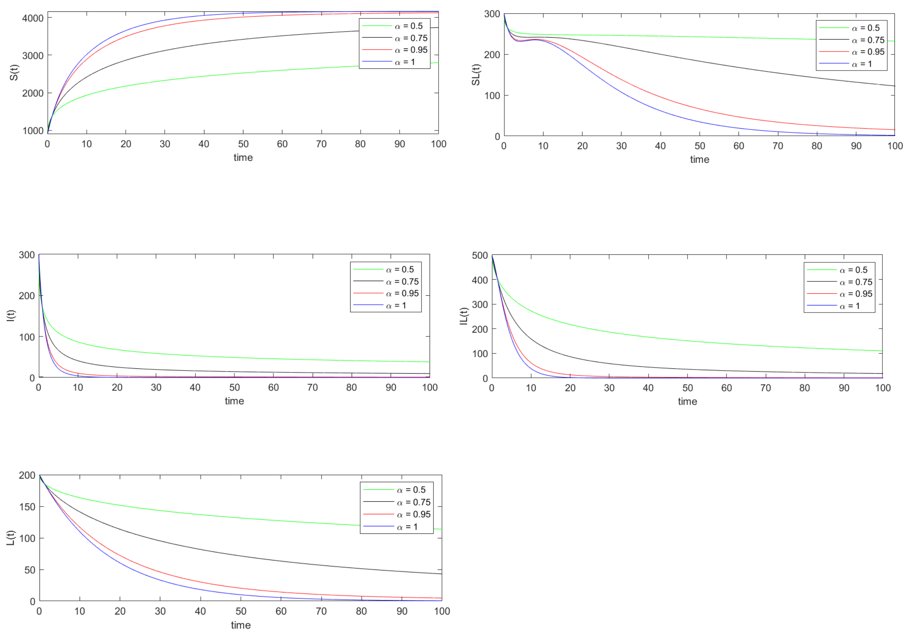
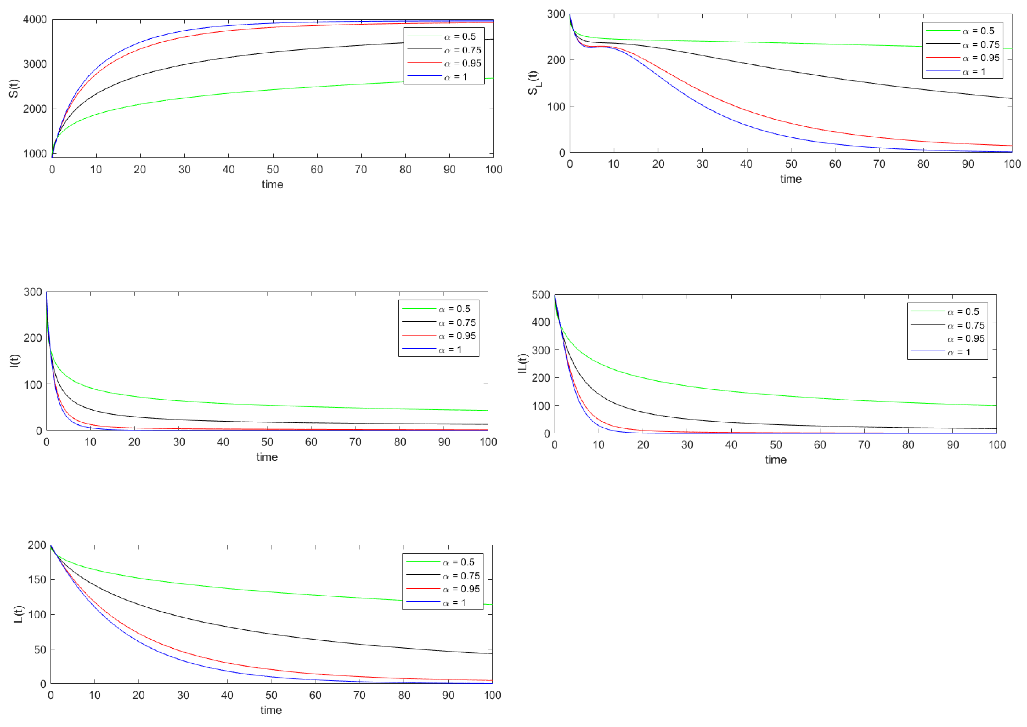
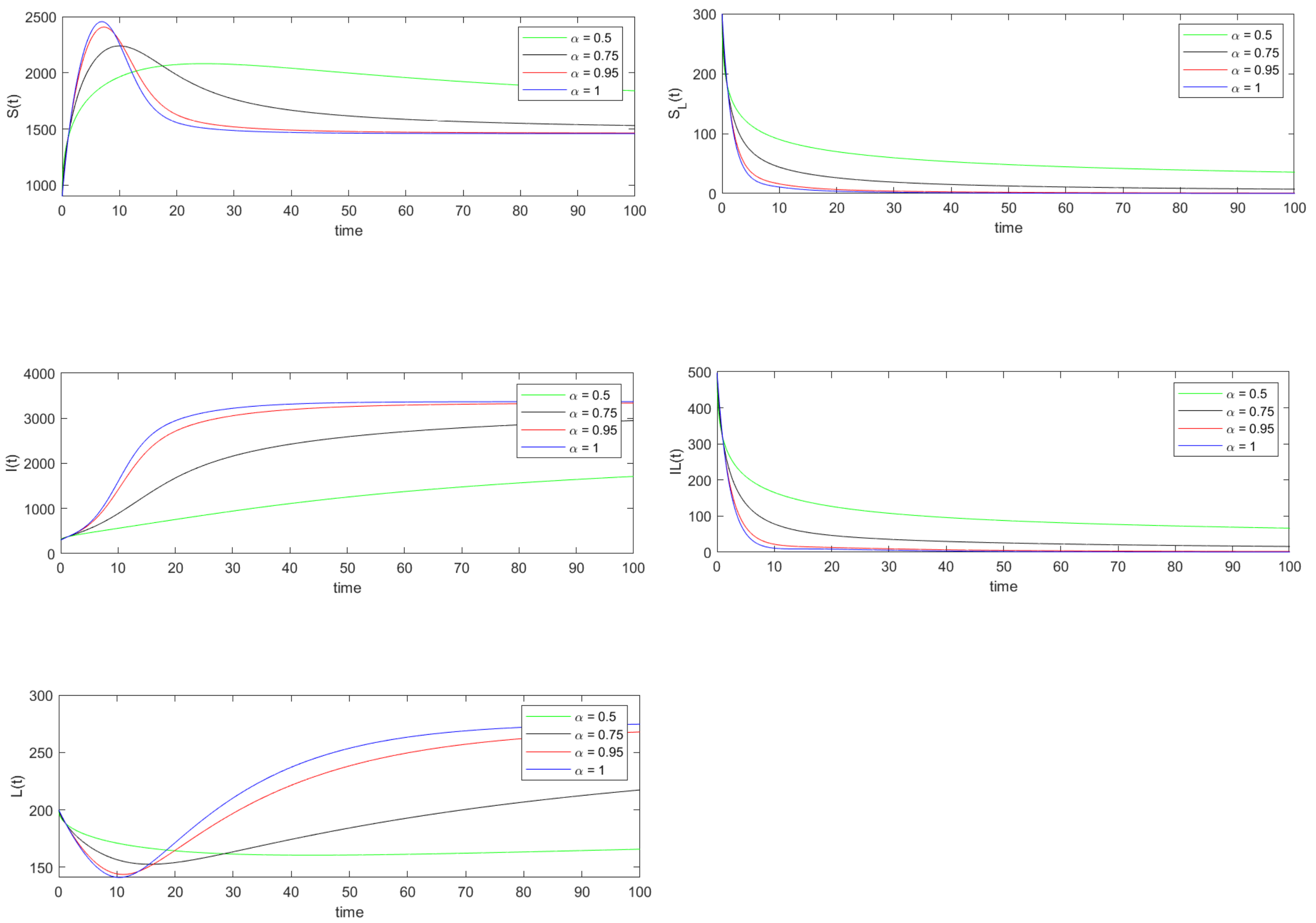
6. Numerical Simulations and Examples

The following table provides the description of the different parameters used in the COVID-19 model. The parameter values under column “data set 1” yield a basic reproduction number ${\mathcal{R}}_0=0.2373$. Similarly, if the parameters under the column “data set 2” are used, then we have ${\mathcal{R}}_0=4.5707$. In Section 6.1, we simulate both the exact and approximated solutions of system (8) using the values under “data set 1” of Table 2 for various $\alpha$ values ($\alpha =0.5,0.75,0.95$ and 1). In Section 6.2, we simulate the exact and approximated solutions of system (8) using the parameter values under “data set 2” of table Table 2. Moreover, in both cases (${\mathcal{R}}_0<1\mathrm{and}{\mathcal{R}}_0>1$) the relative errors, due to approximating the exact solution of system (8) by the residual power series method, are computed for different $\alpha$ values as indicated in Table 3 and Table 4.

Table 2. Input parameter values used to simulate the trajectories of the solution of the model as shown in Figure 1, Figure 2, Figure 3 and Figure 4. The parameters under the column data set 1 will result ${\mathcal{R}}_0=0.2373<1$, and the parameters under data set 2 yield ${\mathcal{R}}_0=4.5707>1.$

Parameters	Description of the Parameters	Data Set 1	Data Set 2	Reference
$\mathsf{\Lambda }$	Recruitment rate	400	400	[38,43]
$\beta$	Infection contact rate	$1.7\times {10}^{-5}$	$1.8\times {10}^{-4}$	[44]
${\lambda }_1$	Imposition of lockdown on susceptible group	$2\times {10}^{-4}$	$2\times {10}^{-5}$	[38,43]
${\lambda }_2$	Imposition of lockdown on infected group	0.002	0.002	[38,43]
${\gamma }_1$	Recovery rate of the infected group	0.16979	0.16979	[38,43]
${\gamma }_2$	Recovery rate of the infected group under lockdown	0.16979	0.16979	[38,43]
${\alpha }_1$	Death rate of the infected group	0.03275	0.03275	[44]
${\alpha }_2$	Death rate of the infected group under lockdown	0.03275	0.03275	[44]
d	Natural death rates	0.096	0.06	[38,43]
${\theta }_1$	Rate of transfer of susceptible lockdown individuals to susceptible class	0.2	0.52	[38,43]
${\theta }_2$	Rate of transfer of susceptible lockdown individuals to infected class	$0.02$	0.2	[38,43]
$\mu$	rate of implementation of the lockdown program	$5\times {10}^{-4}$	$5\times {10}^{-5}$	[38,43]
$\varphi$	rate of depletion of the lockdown program	0.06	0.06	[38,43]

Table 3. Relative error of the state variables for different values of $\alpha$ when ${\mathcal{R}}_0<1$.

	$\mathit{\alpha }=0.5$	$\mathit{\alpha }=0.75$	$\mathit{\alpha }=0.95$	$\mathit{\alpha }=1$
S	$3.876\times {10}^{-6}$	$3.143\times {10}^{-6}$	$2.025\times {10}^{-6}$	$1.202\times {10}^{-6}$
$S_L$	$4.302\times {10}^{-6}$	$2.710\times {10}^{-6}$	$7.094\times {10}^{-7}$	$4.851\times {10}^{-7}$
I	$6.813\times {10}^{-7}$	$2.421\times {10}^{-7}$	$8.059\times {10}^{-8}$	$3.140\times {10}^{-8}$
$I_L$	$1.783\times {10}^{-6}$	$0.448\times {10}^{-6}$	$2.220\times {10}^{-7}$	$1.504\times {10}^{-7}$
L	$1.570\times {10}^{-6}$	$2.097\times {10}^{-6}$	$1.313\times {10}^{-6}$	$9.177\times {10}^{-7}$

Table 4. Relative error of the state variables for different values of $\alpha$ when ${\mathcal{R}}_0>1$.

	$\mathit{\alpha }=0.5$	$\mathit{\alpha }=0.75$	$\mathit{\alpha }=0.95$	$\mathit{\alpha }=1$
S	$4.013\times {10}^{-6}$	$1.571\times {10}^{-6}$	$3.014\times {10}^{-7}$	$2.624\times {10}^{-7}$
$S_L$	$8.201\times {10}^{-5}$	$2.930\times {10}^{-5}$	$5.466\times {10}^{-6}$	$2.181\times {10}^{-6}$
I	$1.099\times {10}^{-6}$	$8.205\times {10}^{-7}$	$3.272\times {10}^{-7}$	$6.142\times {10}^{-8}$
$I_L$	$4.240\times {10}^{-6}$	$3.279\times {10}^{-6}$	$1.142\times {10}^{-6}$	$8.529\times {10}^{-7}$
L	$5.014\times {10}^{-5}$	$1.792\times {10}^{-5}$	$7.263\times {10}^{-6}$	$1.817\times {10}^{-6}$

6.1. Exact and Approximated Solutions of System (8) When ${\mathcal{R}}_0<1$

Using data set 1, the basic reproduction number ${\mathcal{R}}_0$ is calculated to be 0.2373. Thus by Theorems 4 and 5, the disease-free equilibrium point is both locally and globally asymptotically stable. The disease-free equilibrium point is calculated to be $E_0=(4167,0,0,0,0)$. The simulations in Figure 1 and Figure 2 support the fact that the trajectories of system (8) converges to this equilibrium point $E_0=(4167,0,0,0,0)$.

Figure 1. Numerical simulation of the trajectories of the solution of system (8) when ${\mathcal{R}}_0<1.$

Figure 2. Approximated solution of system (8) using the residual power series method when ${\mathcal{R}}_0<1.$ Note that the values of the parameters used in this figure are the same as the one in Figure 1.

In Figure 1 and Figure 2 the exact and approximated solutions of system (8) are plotted for $0\le t\le 100$, respectively. In order to show the accuracy of the residual power series method for approximating the solution of system (8), we have calculated the relative error of each state variable for various $\alpha$ values. A time step size $\Delta t=2^{-6}$ is considered and for each state variables $x\left(t\right)\in \{S\left(t\right),S_L\left(t\right),I\left(t\right),I_L\left(t\right),L\left(t\right)\}$ the values $x(i\Delta t)$ are calculated where $0\le i\le 6400.$ The relative error for the state variable $x\left(t\right)$ is computed using

$$Re{l}_{x\left(t\right)}=\underset{0\le i\le 6400}{max}\left\{\frac{\left|Exact\right(x(i\Delta t))-Appr(x(i\Delta t)\left)\right|}{Exact\left(x\right(i\Delta t\left)\right)}\right\},$$

(33)

where $Exact\left(x\right(i\Delta t\left)\right)$ and $Appr\left(x\right(i\Delta t\left)\right)$ represent the exact and approximated values of the variable $x\left(t\right)$ at $t=i\Delta t$ for $0\le i\le 6400.$ As can be seen from Table 3, the relative error of each state variable decreases as the value of $\alpha$ increases from 0.5 to 1.

6.2. Exact and Approximated Solutions of System (8) When ${\mathcal{R}}_0>1$

The basic reproduction number is calculated using the parameter values under data set 2. The value of ${\mathcal{R}}_0$ is found to be 4.5707, and also the condition ${\lambda }_2<{\theta }_2$ is satisfied. Thus by Remark 6 and Theorem 7 the endemic equilibrium point $E_1=(1458,0,3370,0,0)$, which is calculated using Equation (10), is both locally and globally asymptotically stable. Note that both Figure 3 and Figure 4 show that the trajectories of the solution of system (8) converges to the equilibrium point $E_1$.

Figure 3. Numerical simulation of the trajectories of the solution of system (8) when ${\mathcal{R}}_0>1.$

Figure 4. Approximated solution of system (8) using the residual power series method when ${\mathcal{R}}_0>1.$ The values of the parameters used in this figure are the same as in Figure 3.

Similar to the previous discussion, the relative errors of the state variables are calculated for various $\alpha$ values using Equation (33).

7. Conclusions and Discussion

In this paper, a fractional-order COVID-19 epidemic model with lockdown is proposed and analyzed. In particular, some of the most important epidemiological constants, such as the equilibrium points ($E_0,E_1$ and $E_2$) and the basic reproduction number ${\mathcal{R}}_0$, are calculated. The existence and uniqueness of a positive global solution of the fractional-order system (8) is established. Moreover, by implementing various techniques such as the comparison theory of fractional-order differential equations, Mittage-Leffler stability (Theorem 5), and fractional La-Salle invariance principle (Theorem 6), the local and global stabilities of the equilibrium points are discussed. Additionally, the method of residual power series is used to approximate the solution of system (8). As can be seen in Equation (32), the coefficients $a_n,b_n,c_n,d_n$ and $e_n$ have recursive nature. That is, for any $n\ge 1$, each coefficients $a_n,b_n,c_n,d_n$ and $e_n$ can be determined from the previous ones $a_{n-1},b_{n-1},c_{n-1},d_{n-1}$ and $e_{n-1}$. Thus we can calculate as many coefficients as we need in order to get a very good approximation of the solution of system (8). Moreover, it is very interesting to note that as the value of $\alpha$ increases from 0.5 to 1, the trajectories of the solution of the fractional-order system are converging to the case where $\alpha =1$. That is, the solutions of the fractional-order differential equation converge to the solutions of the system of the ordinary differential equation as the order $\alpha$ increases towards 1. In Section 5, numerical simulations and examples are presented to show the stability of the equilibrium points when ${\mathcal{R}}_0<1$ and ${\mathcal{R}}_0>1.$ The exact solutions of system (8) for various $\alpha$ values are shown in Figure 1 and Figure 3. Similarly, the approximated solutions of system (8) using the residual power series method are included in Figure 2 and Figure 4. Finally, in order to see the accuracy of the approximated solutions, we provided the relative errors for different $\alpha$ values as shown in Table 3 and Table 4. The model that is studied in this paper can be used to predict and understand how COVID-19 infection spreads in the presence of a lockdown. In addition to understanding the dynamics of the infection, it is very important to determine the relative importance of the various parameters used in the model. One such technique is the study of the sensitivity of the parameters in relation to the basic reproduction number ${\mathcal{R}}_0$, and the two endemic equilibrium points $E_1$ and $E_2$, which are considered to be the most important values in the study of deterministic epidemic models. One such approach is to calculate the normalized sensitivity index (NSI), denoted by $S{I}_{\kappa }$, where $\kappa$ is the given parameter. For example, if $\kappa$ is one of the parameters in ${\mathcal{R}}_0$, then the NSI of $\kappa$ is defined as $S{I}_{\kappa }=\frac{\kappa }{{\mathcal{R}}_0}\frac{\partial {\mathcal{R}}_0}{\partial \kappa }.$ Using this result, we have calculated the NSI of the parameters $\beta$ and ${\gamma }_1,$ which are directly affected by the infection. As a result, we have $S{I}_{\beta }=1$, and $S{I}_{{\gamma }_1}=\frac{-{\gamma }_1}{{\gamma }_1+{\alpha }_1+d}<0.$ Thus in order to decrease ${\mathcal{R}}_0$, the expected number of infections generated by one case, we have to either decrease the infection contact rate $\beta$ or increase the recovery rate of the infected group ${\gamma }_1.$ This further implies imposing some prevention actions, such as avoiding contact with people who are infected, wearing masks, and keeping a distance from an infectious person, will help to decrease the value of ${\mathcal{R}}_0$, which directly leads to mitigating the infection. By modifying this model, one can study other aspects of the infection, such as the impact of vaccination, the effect of population diffusion, and other important factors that determine the transmission and persistence of the infection.

References

- Baleanu, D.; Kai, D.; Enrico, S. Fractional Calculus: Models and Numerical Methods; World Scientific: Singapore, 2012. [Google Scholar]
- Djordjevic, J.; Silva, C.J.; Torres, D.F.M. A stochastic SICA epidemic model for HIV transmission. Appl. Math. Lett. 2018, 84, 168–175. [Google Scholar] [CrossRef]
- Hajji, M.; Al-Mdallal, Q. Numerical simulations of a delay model for immune system-tumor interaction. Sultan Qaboos Univ. J. Sci. [SQUJS] 2018, 23, 19–31. [Google Scholar] [CrossRef]
- Ndairou, F.; Area, I.; Nieto, J.J.; Silva, C.J.; Torres, D.F.M. Mathematical modeling of zika disease in pregnant women and newborns with microcephaly in Brazil. Math. Meth. Appl. Sci. 2018, 41, 8929–8941. [Google Scholar] [CrossRef]
- Rachah, A.; Torres, D.F.M. Dynamics and optimal control of ebola transmission. Math. Comput. Sci. 2016, 10, 331–342. [Google Scholar] [CrossRef]
- Rihan, F.A.; Al-Mdallal, Q.M.; AlSakaji, H.J.; Hashish, A. A fractional-order epidemic model with time-delay and nonlinear incidence rate. Chaos Solitons Fractals 2019, 126, 97–105. [Google Scholar] [CrossRef]
- Ahmed, N.; Korkmaz, A.; Rafiq, M.; Baleanu, D.; Alshomrani, A.S.; Rehman, M.A.; Iqbal, S. A novel time efficient structure-preserving splitting method for the solution of two-dimensional reaction-diffusion systems. Adv. Differ. Equ. 2020, 2020, 197. [Google Scholar] [CrossRef]
- Arafa, A.A.M.; Rida, S.Z.; Khalil, M. Solutions of fractional-order model of childhood diseases with constant vaccination strategy. Math. Sci. Lett. 2012, 1, 17–23. [Google Scholar] [CrossRef]
- Baleanu, D.; Mohammadi, H.; Rezapour, S. A mathematical theoretical study of a particular system of caputo fabrizio fractional differential equations for the rubella disease model. Adv. Differ. Equ. 2020, 2020, 184. [Google Scholar] [CrossRef]
- Haq, F.; Shah, K.; Rahman, G.; Shahzad, M. Numerical analysis of fractional order model of HIV-1 infection of CD4+ t-cells. Comput. Method Differ. Equ. 2017, 5, 1–11. [Google Scholar]
- Kumar, D.; Singh, J.; Rathore, S. Application of homotopy analysis transform method to fractional biological population model. Rom. Rep. Phys. 2012, 65, 63–75. [Google Scholar]
- Lia, Y.; Haq, F.; Shah, K.; Shahzad, M.; Rahman, G. Numerical analysis of fractional order pine wilt disease model with bilinear incident rate. J. Math. Comput. Sci. 2017, 17, 420–428. [Google Scholar] [CrossRef]
- Magin, R. Fractional Calculus in Bioengineering; Begell House Publishers: Redding, CT, USA, 2004. [Google Scholar]
- Podlubny, I. Fractional Differential Equations; Academic Press: San Diego, CA, USA, 1998. [Google Scholar]
- Samko, S.G.; Kilbas, A.A.; Marichev, O.I. Fractional Integrals and Derivatives; Gordon and Breach Science Publishers: Yverdon-les-Bains, Switzerland, 1993; Volume 1. [Google Scholar]
- Aba Oud, M.A.A.; Ali, A.; Alrabaiah, H.; Ullah, S.; Khan, M.A. A fractional order mathematical model for COVID-19 dynamics with quarantine, isolation, and environmental viral load. Adv. Differ. Equ. 2021, 2021, 106. [Google Scholar] [CrossRef]
- Ahmed, I.; Baba, I.A.; Yusuf, A.; Kumam, P.; Kumam, W. Analysis of Caputo fractional-order model for COVID-19 with lockdown. Adv. Differ. Equ. 2020, 2020, 394. [Google Scholar] [CrossRef]
- Abdo, M.S.; Shah, K.; Wahash, H.A.; Panchal, S.K. On a comprehensive model of thenovel coronavirus (COVID-19) under mittag-leffler derivative. Chaos Solitons Fractals 2020, 135, 109867. [Google Scholar] [CrossRef]
- Borah, M.; Roy, K.B.; Kapitaniak, T.; Rajagopal, K.; Volos, C. A revisit to the past plague epidemic (India) versus the present COVID-19 pandemic: Fractional-order chaotic. models and fuzzy logic control. Eur. Phys. J. Spec. Top. 2022, 231, 905–919. [Google Scholar] [CrossRef]
- Bahloul, M.A.; Chahid, A.; Laleg-Kirati, T.-M. Fractional-order SEIQRDP model for simulating the dynamics of COVID-19 epidemic. IEEE Open J. Eng. Med. Biol. 2020, 1, 249–256. [Google Scholar] [CrossRef]
- Debbouche, N.; Ouannas, A.; Batiha, I.M.; Grassi, G. Chaotic dynamics in a novel COVID-19 pandemic model described by commensurate and incommensurate fractional-order derivatives. Nonlinear Dyn. 2022, 109, 33–45. [Google Scholar] [CrossRef]
- Li, X.-P.; Bayatti, H.A.; Din, A.; Zeb, A. A vigorous study of fractional-order model via ABC derivatives. Results Phys. 2021, 29, 104737. [Google Scholar] [CrossRef]
- Khan, M.A.; Atangana, A. Modeling the dynamics of novel coronavirus (2019-NCOV) with fractional derivative. Alex. Eng. J. 2020, 59, 2379–2389. [Google Scholar] [CrossRef]
- Shah, K.; Abdeljawad, T.; Mahariq, I.; Jarad, F. Qualitative analysis of a mathematical model in the time of COVID-19. Biomed Res. Int. 2020, 2020, 5098598. [Google Scholar] [CrossRef]
- Zeb, A.; Atangana, A.; Khan, Z.A.; Djillali, S. A robust study of a piecewise fractional order COVID-19 mathematical model. Alex. J. Eng. 2022, 61, 5649–5665. [Google Scholar] [CrossRef]
- Zeb, A.; Kumar, P.; Erturk, V.S.; Sitthiwirattham, T. A new study on two different vaccinated fractional-order COVID-19 models via numerical algorithms. J. King Saud Univ.-Sci. 2022, 34, 101914. [Google Scholar] [CrossRef] [PubMed]
- Zhang, Z.; Zeb, A.; Egbelowo, O.F.; Erturk, V.S. Dynamics of a fractional order mathematical model for COVID-19 epidemic. Adv. Differ. Equ. 2020, 2020, 420. [Google Scholar] [CrossRef] [PubMed]
- El-Ajou, A.; Abu Arqub, O.; Al Zhour, Z.; Momani, S. New results on fractional power series: Theories and applications. Entropy 2013, 15, 5305–5323. [Google Scholar] [CrossRef]
- Caputo, M.; Fabrizio, M. A new definition of fractional derivative without singular kernel. Prog. Fract. Differ. Appl. 2015, 1, 1–13. [Google Scholar]
- Atangana, A.; Baleanu, D. New fractional derivatives with non-local and non-singular kernel. Therm. Sci. 2016, 20, 763–769. [Google Scholar] [CrossRef]
- Hattaf, K. A new generalized definition of fractional derivative with non-singular kernel. Computation 2020, 8, 49. [Google Scholar] [CrossRef]
- Gorenflo, R.; Kilbas, A.A.; Mainardi, F.; Rogosin, S.V. Mittag-Leffler Functions, Related Topics and Applications; Springer: Berlin/Heidelberg, Germany, 2014. [Google Scholar]
- Baba, I.A.; Yusuf, A.; Nisar, K.S.; Abdel-Aty, A.-H.; Nofal, T.A. Mathematical model to assess the imposition of lockdown during COVID-19 pandemic. Results Phys. 2021, 20, 103716. [Google Scholar] [CrossRef] [PubMed]
- Lin, W. Global existence theory and chaos control of fractional differential equations. J. Math. Anal. Appl. 2007, 323, 709–726. [Google Scholar] [CrossRef]
- Diekmann, O.; Heesterbeek, J.A.P.; Metz, J.A.P. On the definition and the computation of the basic reproduction ratio R0 in models for infectious diseases in heterogeneous populations. J. Math. Biol. 1990, 28, 365–382. [Google Scholar] [CrossRef]
- Matignon, D. Stability Results for Fractional Differential Equations with Applications to Control Processing; Computational Engineering in Systems Applications: Lille, France, 1996; Volume 2, pp. 963–968. [Google Scholar]
- Li, Y.; Chen, Y.; Podlubny, I. Mittag–Leffler stability of fractional order nonlinear dynamic systems. Automatica 2009, 45, 1965–1969. [Google Scholar] [CrossRef]
- Li, Y.; Chen, Y.; Podlubny, I. Stability of fractional-order nonlinear dynamic systems: Lyapunov direct method and generalized Mittag–Leffler stability. Comput. Math. Appl. 2010, 59, 1810–1821. [Google Scholar] [CrossRef]
- Hattaf, K. On the stability and numerical scheme of fractional differential equations with application to biology. Computation 2022, 10, 97. [Google Scholar] [CrossRef]
- Delavari, H.; Baleanu, D.; Sadati, J. Stability analysis of Caputo fractional-order nonlinear systems revisited. Nonlinear Dyn. 2012, 67, 2433–2439. [Google Scholar] [CrossRef]
- Hattaf, K. Dynamics of a generalized fractional epidemic model of COVID-19 with carrier effect. Adv. Syst. Sci. Appl. 2022, 22, 36–48. [Google Scholar]
- Hasan, S.; Al-Zoubi, A.; Freihet, A.; Al-Smadi1, M.; Momani, S. Solution of fractional SIR epidemic Model using residual power series method. Appl. Math. Inf. Sci. 2019, 13, 153–161. [Google Scholar] [CrossRef]
- Yang, H.M.; Lombardi Junior, L.P.; Castro, F.F.M.; Yang, A.C. Mathematical modeling of the transmission of SARS-CoV-2—Evaluating the impact of isolation in São Paulo State (Brazil) and lockdown in Spain associated with protective measures on the epidemic of COVID-19. PLoS ONE 2021, 16, e0252271. [Google Scholar] [CrossRef]
- Rothe, C.; Schunk, M.; Sothmann, P.; Bretzel, G.; Froeschl, G.; Wallrauch, C.; Zimmer, T.; Thiel, V.; Janke, C.; Guggemos, W. Transmission of 2019-nCoV infection from an asymptomatic contact in Germany. N. Engl. J. Med. 2020, 382, 970–971. [Google Scholar] [CrossRef]
Publisher’s Note: MDPI stays neutral with regard to jurisdictional claims in published maps and institutional affiliations. |
© 2022 by the authors. Licensee MDPI, Basel, Switzerland. This article is an open access article distributed under the terms and conditions of the Creative Commons Attribution (CC BY) license (https://creativecommons.org/licenses/by/4.0/).