

Exploring Abnormal Brain Functional Connectivity in Healthy Adults, Depressive Disorder, and Generalized Anxiety Disorder through EEG Signals: A Machine Learning Approach for Triple Classification
 , ,
, ,
Abstract
1. Introduction
2. Materials and Methods
2.1. Participants and Materials
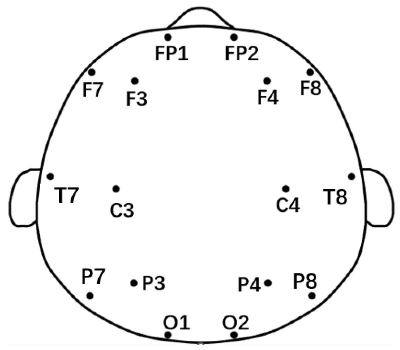
2.2. EEG Data Acquisition and Preprocessing
2.3. Feature Extraction
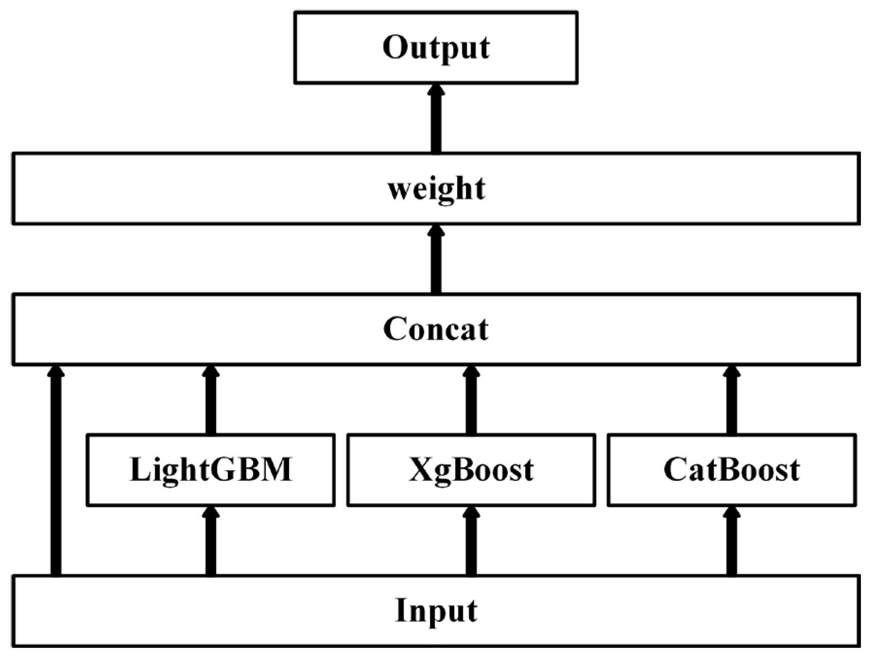
2.4. Machine Learning
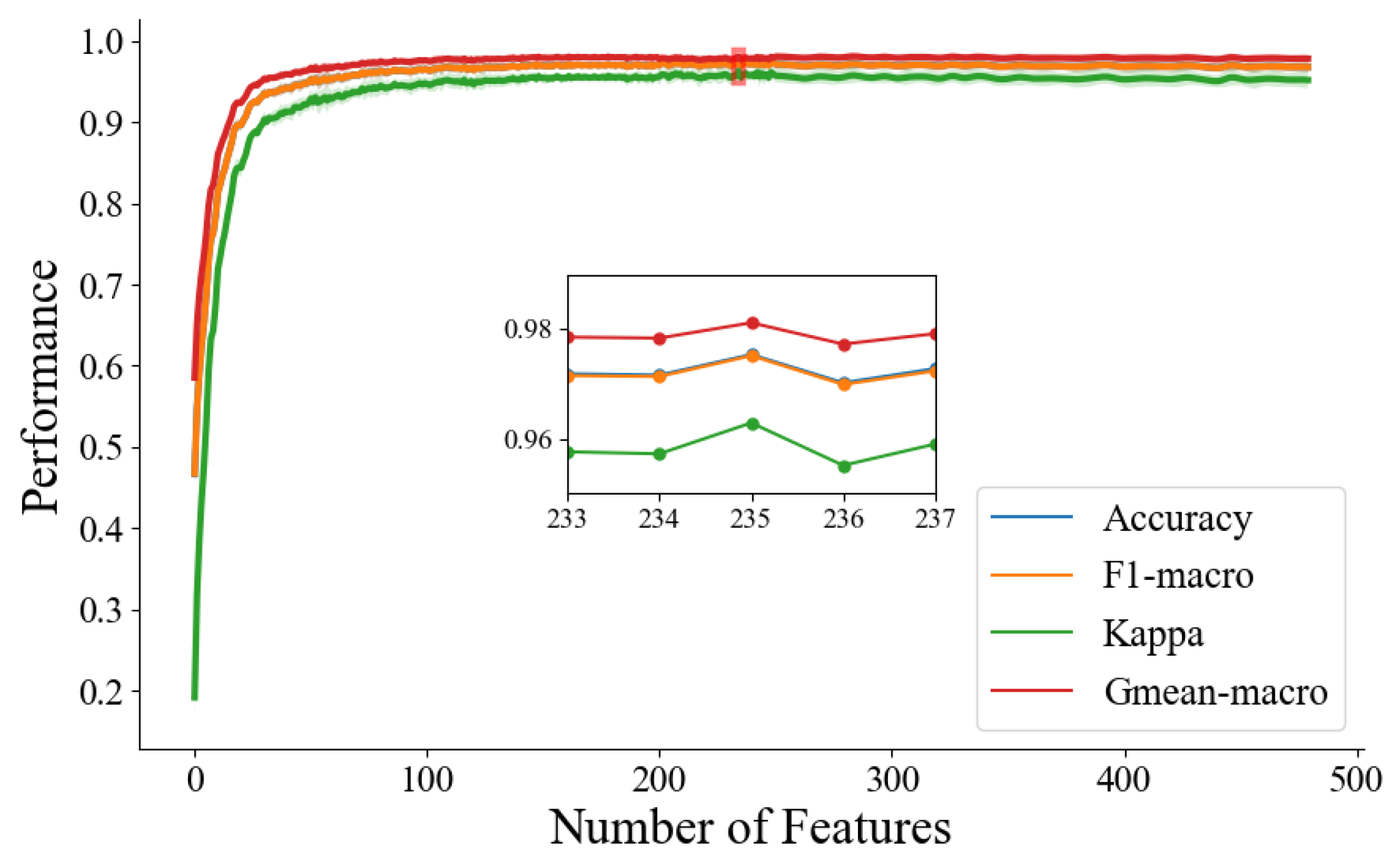
2.5. Feature Selection
2.6. Parameter Optimization
2.7. Evaluating Indicator
3. Results
4. Discussion
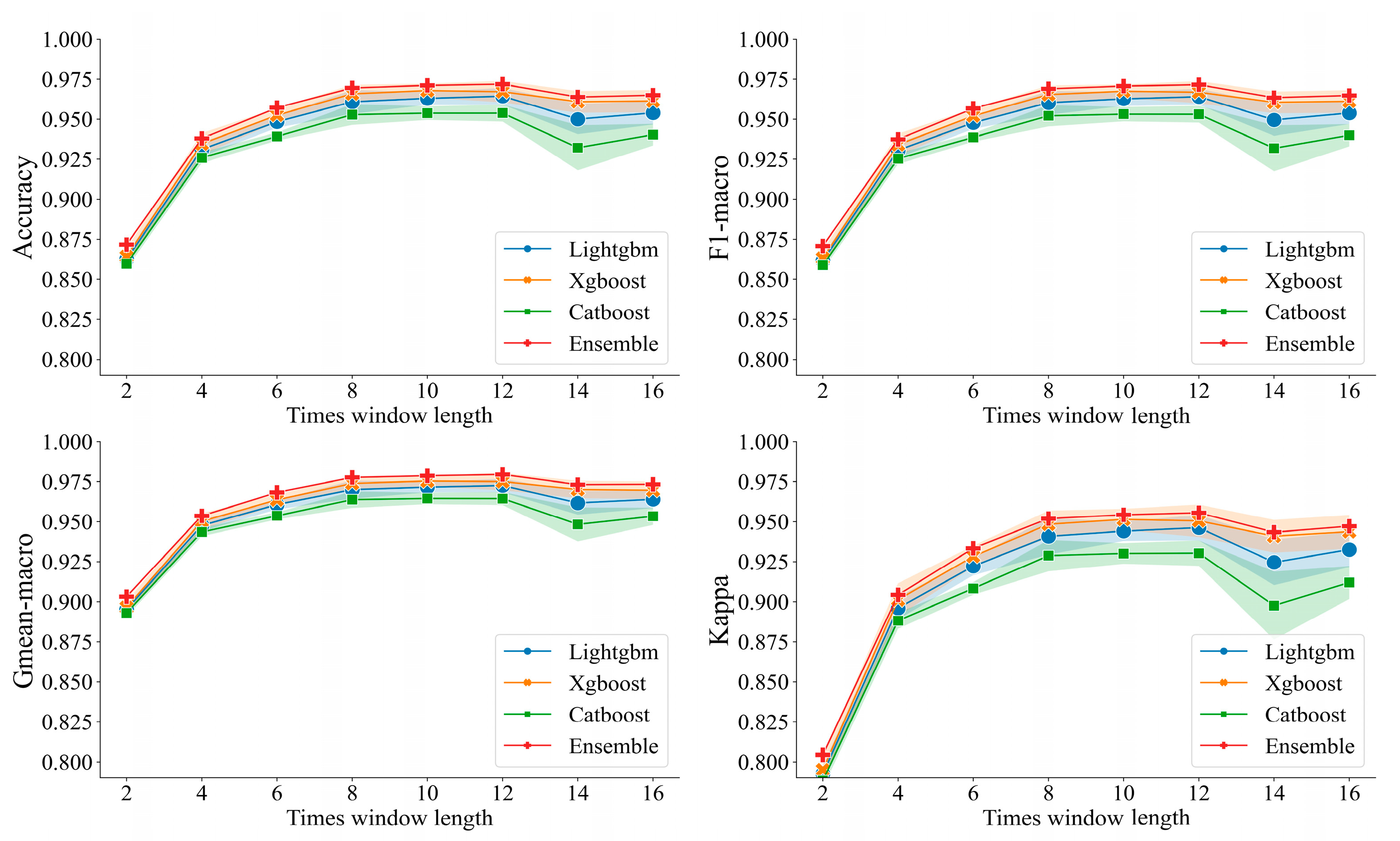
4.1. Appropriate Time Window Achieves Optimal Classification Performance
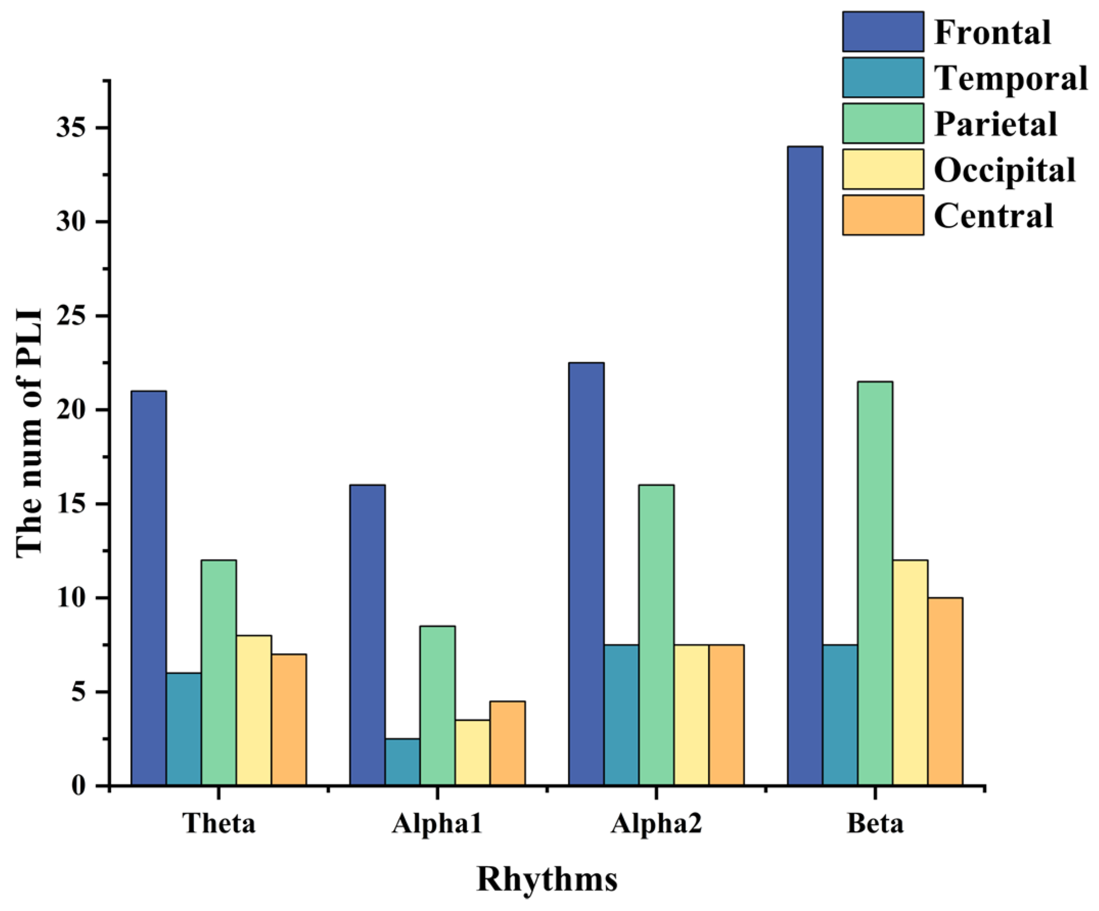
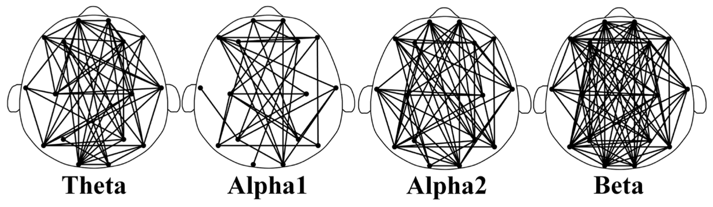
4.2. General Patterns of Brain Reorganization among Three Groups
4.3. The Feasibility of Machine Learning for Psychiatric Disorder Diagnosis
4.4. Limitations
5. Conclusions
Author Contributions
Funding
Institutional Review Board Statement
Informed Consent Statement
Data Availability Statement
Conflicts of Interest
References
- Cai, H.; Han, J.; Chen, Y.; Sha, X.; Wang, Z.; Hu, B.; Yang, J.; Feng, L.; Ding, Z.; Chen, Y.; et al. A Pervasive Approach to EEG-Based Depression Detection. Complexity 2018, 2018, 5238028. [Google Scholar] [CrossRef]
- Ruscio, A.M.; Hallion, L.S.; Lim, C.C.W.; Aguilar-Gaxiola, S.; Al-Hamzawi, A.; Alonso, J.; Andrade, L.H.; Borges, G.; Bromet, E.J.; Bunting, B.; et al. Cross-sectional Comparison of the Epidemiology of DSM-5 Generalized Anxiety Disorder across the Globe. JAMA Psychiatry 2017, 74, 465–475. [Google Scholar] [CrossRef] [PubMed]
- Santomauro, D.F.; Herrera, A.M.M.; Shadid, J.; Zheng, P.; Ashbaugh, C.; Pigott, D.M.; Abbafati, C.; Adolph, C.; Amlag, J.O.; Aravkin, A.Y.; et al. Global prevalence and burden of depressive and anxiety disorders in 204 countries and territories in 2020 due to the COVID-19 pandemic. Lancet 2021, 398, 1700–1712. [Google Scholar] [CrossRef] [PubMed]
- Polanczyk, G.; de Lima, M.S.; Horta, B.L.; Biederman, J.; Rohde, L.A. The worldwide prevalence of ADHD: A systematic review and metaregression analysis. Am. J. Psychiatry 2007, 164, 942–948. [Google Scholar] [CrossRef] [PubMed]
- Miljevic, A.; Bailey, N.W.; Murphy, O.W.; Perera, M.P.N.; Fitzgerald, P.B. Alterations in EEG functional connectivity in individuals with depression: A systematic review. J. Affect. Disord. 2023, 328, 287–302. [Google Scholar] [CrossRef]
- American Psychiatric Publishing, Inc. Diagnostic and Statistical Manual of Mental Disorders: DSM-5™, 5th ed.; American Psychiatric Publishing, Inc.: Arlington, VA, USA, 2013; p. xliv, 947. [Google Scholar]
- Cummings, C.M.; Caporino, N.E.; Kendall, P.C. Comorbidity of Anxiety and Depression in Children and Adolescents: 20 Years After. Psychol. Bull. 2014, 140, 816–845. [Google Scholar] [CrossRef] [PubMed]
- Newson, J.J.; Thiagarajan, T.C. EEG Frequency Bands in Psychiatric Disorders: A Review of Resting State Studies. Front. Hum. Neurosci. 2019, 12, 521. [Google Scholar] [CrossRef]
- Seal, A.; Bajpai, R.; Karnati, M.; Agnihotri, J.; Yazidi, A.; Herrera-Viedma, E.; Krejcar, O. Benchmarks for machine learning in depression discrimination using electroencephalography signals. Appl. Intell. 2023, 53, 12666–12683. [Google Scholar] [CrossRef]
- Crosson, B.; Ford, A.; McGregor, K.M.; Meinzer, M.; Cheshkov, S.; Li, X.; Walker-Batson, D.; Briggs, R.W. Functional imaging and related techniques: An introduction for rehabilitation researchers. J. Rehabil. Res. Dev. 2010, 47, VII–XXXIII. [Google Scholar] [CrossRef]
- Li, G.; Zhong, H.; Wang, J.; Yang, Y.; Li, H.; Wang, S.; Sun, Y.; Qi, X. Machine Learning Techniques Reveal Aberrated Multidimensional EEG Characteristics in Patients with Depression. Brain Sci. 2023, 13, 384. [Google Scholar] [CrossRef] [PubMed]
- Qi, X.; Xu, W.; Li, G. Neuroimaging Study of Brain Functional Differences in Generalized Anxiety Disorder and Depressive Disorder. Brain Sci. 2023, 13, 1282. [Google Scholar] [CrossRef] [PubMed]
- Qi, X.; Fang, J.; Sun, Y.; Xu, W.; Li, G. Altered Functional Brain Network Structure between Patients with High and Low Generalized Anxiety Disorder. Diagnostics 2023, 13, 1292. [Google Scholar] [CrossRef] [PubMed]
- Wang, R.; Wang, J.; Yu, H.; Wei, X.; Yang, C.; Deng, B. Power spectral density and coherence analysis of Alzheimer’s EEG. Cogn. Neurodyn. 2015, 9, 291–304. [Google Scholar] [CrossRef]
- Yao, W.-P.; Liu, T.-B.; Dai, J.-F.; Wang, J. Multiscale permutation entropy analysis of electroencephalogram. Acta Phys. Sin. 2014, 63, 078704. [Google Scholar] [CrossRef]
- Peraza, L.R.; Asghar, A.U.R.; Green, G.; Halliday, D.M. Volume conduction effects in brain network inference from electroencephalographic recordings using phase lag index. J. Neurosci. Methods 2012, 207, 189–199. [Google Scholar] [CrossRef]
- Wang, J.; Fang, J.; Xu, Y.; Zhong, H.; Li, J.; Li, H.; Li, G. Difference analysis of multidimensional electroencephalogram characteristics between young and old patients with generalized anxiety disorder. Front. Hum. Neurosci. 2022, 16, 1074587. [Google Scholar] [CrossRef]
- Wang, S.-Y.; Lin, I.M.; Fan, S.-Y.; Tsai, Y.-C.; Yen, C.-F.; Yeh, Y.-C.; Huang, M.-F.; Lee, Y.; Chiu, N.-M.; Hung, C.-F.; et al. The effects of alpha asymmetry and high-beta down-training neurofeedback for patients with the major depressive disorder and anxiety symptoms. J. Affect. Disord. 2019, 257, 287–296. [Google Scholar] [CrossRef]
- Arns, M.; Conners, C.K.; Kraemer, H.C. A Decade of EEG Theta/Beta Ratio Research in ADHD: A Meta-Analysis. J. Atten. Disord. 2013, 17, 374–383. [Google Scholar] [CrossRef]
- Guo, Z.; Wu, X.; Liu, J.; Yao, L.; Hu, B. Altered electroencephalography functional connectivity in depression during the emotional face-word Stroop task. J. Neural Eng. 2018, 15, 056014. [Google Scholar] [CrossRef]
- Shen, Z.; Li, G.; Fang, J.; Zhong, H.; Wang, J.; Sun, Y.; Shen, X. Aberrated Multidimensional EEG Characteristics in Patients with Generalized Anxiety Disorder: A Machine-Learning Based Analysis Framework. Sensors 2022, 22, 5420. [Google Scholar] [CrossRef]
- Sun, S.; Liu, L.; Shao, X.; Yan, C.; Li, X.; Hu, B. Abnormal Brain Topological Structure of Mild Depression During Visual Search Processing Based on EEG Signals. IEEE Trans. Neural Syst. Rehabil. Eng. 2022, 30, 1705–1715. [Google Scholar] [CrossRef] [PubMed]
- Thakre, T.P.; Kulkarni, H.; Adams, K.S.; Mischel, R.; Hayes, R.; Pandurangi, A. Polysomnographic identification of anxiety and depression using deep learning. J. Psychiatr. Res. 2022, 150, 54–63. [Google Scholar] [CrossRef] [PubMed]
- Sau, A.B.I. Predicting anxiety and depression in elderly patients using machine learning technology. Health Technol. Lett. 2017, 4, 238–243. [Google Scholar] [CrossRef]
- Iyortsuun, N.K.; Kim, S.H.; Jhon, M.; Yang, H.J.; Pant, S. A Review of Machine Learning and Deep Learning Approaches on Mental Health Diagnosis. Healthcare 2023, 11, 285. [Google Scholar] [CrossRef] [PubMed]
- Ke, G.; Meng, Q.; Finley, T.; Wang, T.; Chen, W.; Ma, W.; Ye, Q.; Liu, T.-Y. Lightgbm: A highly efficient gradient boosting decision tree. Adv. Neural Inf. Process. Syst. 2017, 30, 3149–3157. [Google Scholar]
- Chen, T.; Guestrin, C. Xgboost: A scalable tree boosting system. In Proceedings of the 22nd ACM SIGKDD International Conference on Knowledge Discovery and Data Mining, San Francisco, CA, USA, 13–17 August 2016; pp. 785–794. [Google Scholar]
- Prokhorenkova, L.; Gusev, G.; Vorobev, A.; Dorogush, A.V.; Gulin, A. CatBoost: Unbiased boosting with categorical features. Adv. Neural Inf. Process. Syst. 2018, 31, 6639–6649. [Google Scholar] [CrossRef]
- Cai, H.; Liu, X.; Ni, R.; Song, S.; Cangelosi, A. Emotion Recognition through Combining EEG and EOG over Relevant Channels with Optimal Windowing. IEEE Trans. Hum.-Mach. Syst. 2023, 53, 697–706. [Google Scholar] [CrossRef]
- Rabinowitz, J.; Williams, J.B.W.; Anderson, A.; Fu, D.J.; Hefting, N.; Kadriu, B.; Kott, A.; Mahableshwarkar, A.; Sedway, J.; Williamson, D.; et al. Consistency checks to improve measurement with the Hamilton Rating Scale for Depression (HAM-D). J. Affect. Disord. 2022, 302, 273–279. [Google Scholar] [CrossRef]
- Erickson, N.; Mueller, J.; Shirkov, A.; Zhang, H.; Larroy, P.; Li, M.; Smola, A. Autogluon-tabular: Robust and accurate automl for structured data. arXiv 2020, arXiv:2003.06505. [Google Scholar]
- Sameen, M.I.; Pradhan, B.; Lee, S. Application of convolutional neural networks featuring Bayesian optimization for landslide susceptibility assessment. Catena 2020, 186, 104249. [Google Scholar] [CrossRef]
- Ouyang, D.; Yuan, Y.; Li, G.; Guo, Z. The Effect of Time Window Length on EEG-Based Emotion Recognition. Sensors 2022, 22, 4939. [Google Scholar] [CrossRef] [PubMed]
- Pereira, E.T.; Gomes, H.M.; Veloso, L.R.; Mota, M.A. Empirical Evidence Relating EEG Signal Duration to Emotion Classification Performance. IEEE Trans. Affect. Comput. 2021, 12, 154–164. [Google Scholar] [CrossRef]
- Lin, Y.-P.; Wang, C.-H.; Jung, T.-P.; Wu, T.-L.; Jeng, S.-K.; Duann, J.-R.; Chen, J.-H. EEG-Based Emotion Recognition in Music Listening. IEEE Trans. Biomed. Eng. 2010, 57, 1798–1806. [Google Scholar] [CrossRef] [PubMed]
- Yu, X.; Li, Z.; Zang, Z.; Liu, Y. Real-Time EEG-Based Emotion Recognition. Sensors 2023, 23, 7853. [Google Scholar] [CrossRef] [PubMed]
- Zhuang, N.; Zeng, Y.; Tong, L.; Zhang, C.; Zhang, H.; Yan, B. Emotion Recognition from EEG Signals Using Multidimensional Information in EMD Domain. BioMed Res. Int. 2017, 2017, 8317357. [Google Scholar] [CrossRef] [PubMed]
- Xing, X.; Li, Z.; Xu, T.; Shu, L.; Hue, B.; Xu, X. SAE plus LSTM: A New Framework for Emotion Recognition From Multi-Channel EEG. Front. Neurorobot. 2019, 13, 37. [Google Scholar] [CrossRef] [PubMed]
- Di Gregorio, F.; Battaglia, S. Advances in EEG-based functional connectivity approaches to the study of the central nervous system in health and disease. Adv. Clin. Exp. Med. 2023, 32, 607–612. [Google Scholar] [CrossRef] [PubMed]
- Baker, A.P.; Brookes, M.J.; Rezek, I.A.; Smith, S.M.; Behrens, T.; Smith, P.J.P.; Woolrich, M. Fast transient networks in spontaneous human brain activity. eLife 2014, 3, e01867. [Google Scholar] [CrossRef]
- Grefkes, C.; Fink, G.R. Connectivity-based approaches in stroke and recovery of function. Lancet Neurol. 2014, 13, 206–216. [Google Scholar] [CrossRef]
- Yasin, S.; Othmani, A.; Raza, I.; Hussain, S.A. Machine learning based approaches for clinical and non-clinical depression recognition and depression relapse prediction using audiovisual and EEG modalities: A comprehensive review. Comput. Biol. Med. 2023, 159, 106741. [Google Scholar] [CrossRef]
- Xie, Y.; Yang, B.; Lu, X.; Zheng, M.; Fan, C.; Bi, X.; Zhou, S.; Li, Y. Anxiety and Depression Diagnosis Method Based on Brain Networks and Convolutional Neural Networks. In Proceedings of the 2020 42nd Annual International Conference of the IEEE Engineering in Medicine & Biology Society (EMBC), Montreal, QC, Canada, 20–24 July 2020; Volume 2020, pp. 1503–1506. [Google Scholar] [CrossRef]
- Pizzagalli, D.A.; Roberts, A.C. Prefrontal cortex and depression. Neuropsychopharmacology 2022, 47, 225–246. [Google Scholar] [CrossRef]
- Chai, Y.; Sheline, Y.I.; Oathes, D.J.; Balderston, N.L.; Rao, H.; Yu, M. Feature Review Functional connectomics in depression: Insights into therapies. Trends Cogn. Sci. 2023, 27, 814–832. [Google Scholar] [CrossRef] [PubMed]
- Seok, D.; Beer, J.; Jaskir, M.; Smyk, N.; Jaganjac, A.; Makhoul, W.; Cook, P.; Elliott, M.; Shinohara, R.; Sheline, Y.I. Differential Impact of Anxious Misery Psychopathology on Multiple Representations of the Functional Connectome. Biol. Psychiatry Glob. Open Sci. 2022, 2, 489–499. [Google Scholar] [CrossRef] [PubMed]
- Barttfeld, P.; Petroni, A.; Baez, S.; Urquina, H.; Sigman, M.; Cetkovich, M.; Torralva, T.; Torrente, F.; Lischinsky, A.; Castellanos, X.; et al. Functional Connectivity and Temporal Variability of Brain Connections in Adults with Attention Deficit/Hyperactivity Disorder and Bipolar Disorder. Neuropsychobiology 2014, 69, 65–75. [Google Scholar] [CrossRef]
- Hosseini, M.-P.; Hosseini, A.; Ahi, K. A Review on Machine Learning for EEG Signal Processing in Bioengineering. IEEE Rev. Biomed. Eng. 2021, 14, 204–218. [Google Scholar] [CrossRef]


| Features | HC | GAD | DD | p |
|---|---|---|---|---|
| Number | 38 | 45 | 42 | - |
| Age (year) | 38.16 ± 12.36 | 41.47 ± 9.38 | 44.55 ± 12.30 | 0.051 |
| Gender (male/female) | 12/26 | 13/32 | 10/32 | 0.74 |
| Time Window (s) | HC | GAD | DD |
|---|---|---|---|
| 2 | 8506 | 10,902 | 9425 |
| 4 | 4163 | 5371 | 4632 |
| 6 | 2628 | 3319 | 2853 |
| 8 | 1971 | 2592 | 2228 |
| 10 | 1530 | 2048 | 1747 |
| 12 | 1301 | 1604 | 1360 |
| 14 | 880 | 1122 | 961 |
| 16 | 873 | 1077 | 906 |
| Model | Parameter | Description |
|---|---|---|
| LightGBM | num_leaves | Uniformint [16,96] |
| min_data_in_leaf | Uniformint [2,60] | |
| feature_fraction | Uniform [0.75,1] | |
| learning_rate | loguniform [log(5 × 10⁻³),log(0.1)] | |
| XGBoost | depth | Uniformint [3,10] |
| min_child_weight | Uniformint [1,5] | |
| colsample_bytree | Uniform [0.5,1.0] | |
| learning_rate | Loguniform [log(5 × 10⁻³),log(0.1)] | |
| CatBoost | max_depth | Uniformint [5,8] |
| l2_leaf_reg | Uniform [1,5] | |
| learning_rate | Loguniform [log(5 × 10⁻³),log(0.1)] |
| Models | Accuracy | F1-Macro | Gmean-Macro | Kappa |
|---|---|---|---|---|
| Lightgbm | 96.44 ± 0.53 | 96.40 ± 0.50 | 94.63 ± 0.80 | 97.26 ± 0.42 |
| Xgboost | 95.38 ± 0.53 | 95.31 ± 0.52 | 93.04 ± 0.80 | 96.45 ± 0.41 |
| Catboost | 96.72 ± 0.68 | 96.69 ± 0.70 | 95.05 ± 1.02 | 97.50 ± 0.54 |
| Ensemble | 96.89 ± 0.51 | 96.86 ± 0.52 | 95.26 ± 0.77 | 97.65 ± 0.41 |
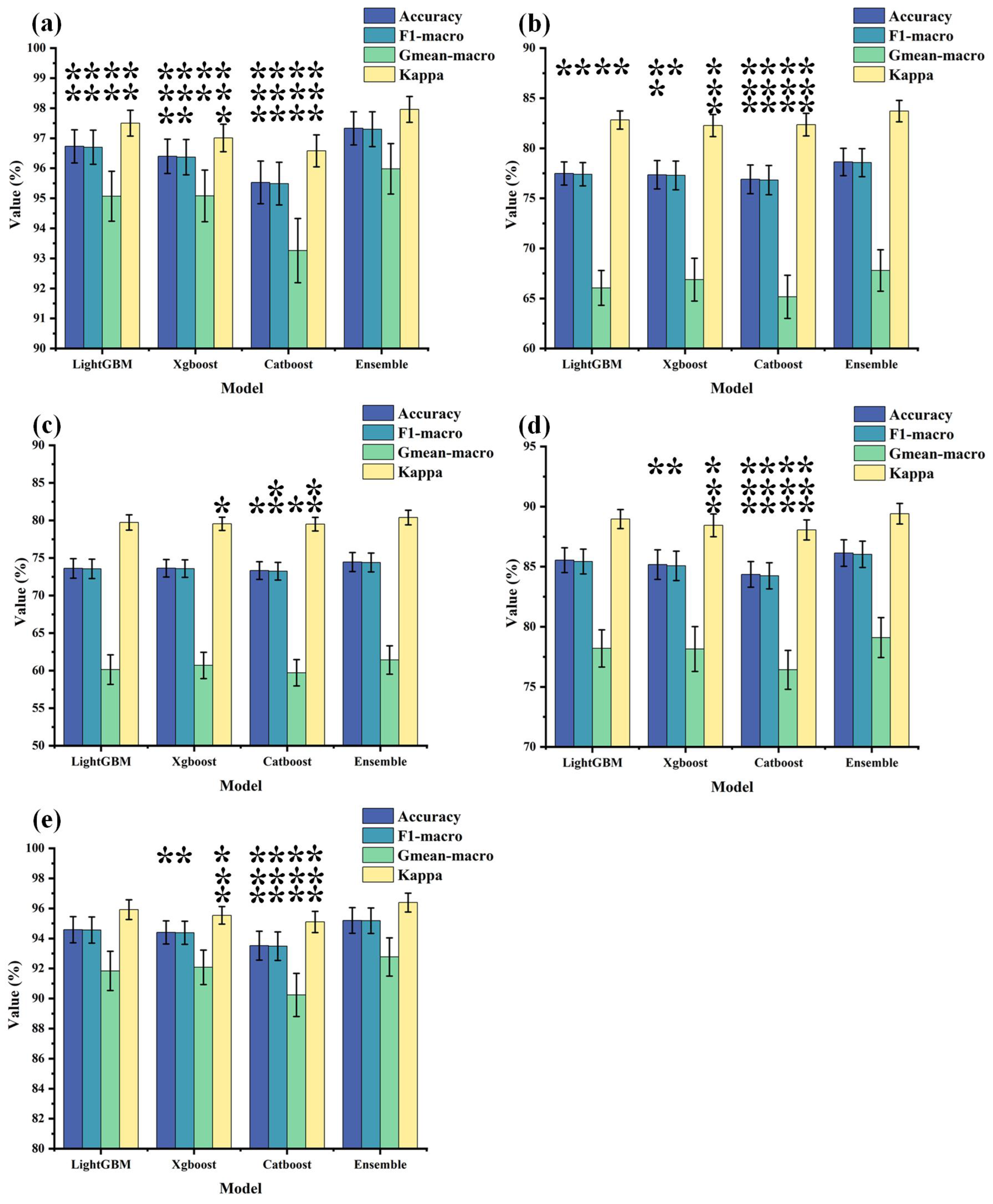
| Rhythm | Model | Accuracy | F1-Macro | Gmean-Macro | Kappa |
|---|---|---|---|---|---|
| All | Lightgbm | 96.73 ± 0.55 | 96.70 ± 0.57 | 95.07 ± 0.83 | 97.50 ± 0.43 |
| Xgboost | 96.40 ± 0.57 | 96.37 ± 0.59 | 95.08 ± 0.86 | 97.01 ± 0.46 | |
| Catboost | 95.53 ± 0.71 | 95.49 ± 0.71 | 93.26 ± 1.07 | 96.58 ± 0.53 | |
| Ensemble | 97.33 ± 0.55 *** | 97.30 ± 0.58 *** | 95.98 ± 0.84 *** | 97.96 ± 0.43 *** | |
| Theta | Ligthgbm | 77.48 ± 1.15 | 77.40 ± 1.16 | 66.05 ± 1.74 | 82.82 ± 0.91 |
| Xgboost | 77.35 ± 1.42 | 77.29 ± 1.43 | 66.87 ± 2.14 | 82.27 ± 1.10 | |
| Catboost | 76.90 ± 1.43 | 76.82 ± 1.46 | 65.16 ± 2.16 | 82.36 ± 1.12 | |
| Ensemble | 78.63 ± 1.37 *** | 78.56 ± 1.40 *** | 67.79 ± 2.07 *** | 83.71 ± 1.07 *** | |
| Alpha1 | Ligthgbm | 73.62 ± 1.30 | 73.56 ± 1.29 | 60.14 ± 1.97 | 79.74 ± 1.02 |
| Xgboost | 73.64 ± 1.17 | 73.59 ± 1.16 | 60.70 ± 1.76 | 79.55 ± 0.89 | |
| Catboost | 73.33 ± 1.17 | 73.24 ± 1.17 | 59.72 ± 1.76 | 79.51 ± 0.90 | |
| Ensemble | 74.46 ± 1.26 * | 74.40 ± 1.26 * | 61.42 ± 1.89 * | 80.39 ± 0.97 ** | |
| Alpha2 | Ligthgbm | 85.54 ± 1.03 | 85.43 ± 1.03 | 78.20 ± 1.55 | 88.97 ± 0.79 |
| Xgboost | 85.18 ± 1.23 | 85.07 ± 1.22 | 78.15 ± 1.87 | 88.44 ± 0.95 | |
| Catboost | 84.36 ± 1.07 | 84.24 ± 1.09 | 76.42 ± 1.62 | 88.06 ± 0.83 | |
| Ensemble | 86.14 ± 1.10 *** | 86.03 ± 1.10 *** | 79.10 ± 1.66 *** | 89.41 ± 0.85 *** | |
| Beta | Ligthgbm | 94.58 ± 0.87 | 94.56 ± 0.87 | 91.84 ± 1.31 | 95.92 ± 0.66 |
| Xgboost | 94.40 ± 0.77 | 94.38 ± 0.77 | 92.08 ± 1.15 | 95.54 ± 0.58 | |
| Catboost | 93.52 ± 0.96 | 93.49 ± 0.95 | 90.24 ± 1.44 | 95.10 ± 0.71 | |
| Ensemble | 95.20 ± 0.85 *** | 95.18 ± 0.85 *** | 92.77 ± 1.27 *** | 96.39 ± 0.63 *** |
Disclaimer/Publisher’s Note: The statements, opinions and data contained in all publications are solely those of the individual author(s) and contributor(s) and not of MDPI and/or the editor(s). MDPI and/or the editor(s) disclaim responsibility for any injury to people or property resulting from any ideas, methods, instructions or products referred to in the content. |
© 2024 by the authors. Licensee MDPI, Basel, Switzerland. This article is an open access article distributed under the terms and conditions of the Creative Commons Attribution (CC BY) license (https://creativecommons.org/licenses/by/4.0/).
Share and Cite
Fang, J.; Li, G.; Xu, W.; Liu, W.; Chen, G.; Zhu, Y.; Luo, Y.; Luo, X.; Zhou, B. Exploring Abnormal Brain Functional Connectivity in Healthy Adults, Depressive Disorder, and Generalized Anxiety Disorder through EEG Signals: A Machine Learning Approach for Triple Classification. Brain Sci. 2024, 14, 245. https://doi.org/10.3390/brainsci14030245
Fang J, Li G, Xu W, Liu W, Chen G, Zhu Y, Luo Y, Luo X, Zhou B. Exploring Abnormal Brain Functional Connectivity in Healthy Adults, Depressive Disorder, and Generalized Anxiety Disorder through EEG Signals: A Machine Learning Approach for Triple Classification. Brain Sciences. 2024; 14(3):245. https://doi.org/10.3390/brainsci14030245
Chicago/Turabian StyleFang, Jiaqi, Gang Li, Wanxiu Xu, Wei Liu, Guibin Chen, Yixia Zhu, Youdong Luo, Xiaodong Luo, and Bin Zhou. 2024. "Exploring Abnormal Brain Functional Connectivity in Healthy Adults, Depressive Disorder, and Generalized Anxiety Disorder through EEG Signals: A Machine Learning Approach for Triple Classification" Brain Sciences 14, no. 3: 245. https://doi.org/10.3390/brainsci14030245
APA StyleFang, J., Li, G., Xu, W., Liu, W., Chen, G., Zhu, Y., Luo, Y., Luo, X., & Zhou, B. (2024). Exploring Abnormal Brain Functional Connectivity in Healthy Adults, Depressive Disorder, and Generalized Anxiety Disorder through EEG Signals: A Machine Learning Approach for Triple Classification. Brain Sciences, 14(3), 245. https://doi.org/10.3390/brainsci14030245