Machine Learning Detects Pattern of Differences in Functional Magnetic Resonance Imaging (fMRI) Data between Chronic Fatigue Syndrome (CFS) and Gulf War Illness (GWI)

 ,
,  ,
,
Abstract

1. Background
2. Methods
2.1. Ethics
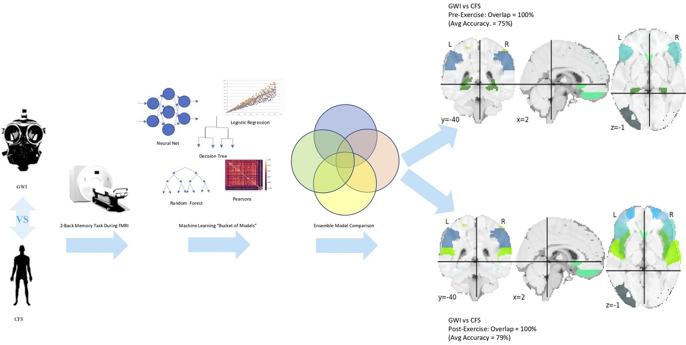
2.2. Approach
2.3. Subjects
2.4. Magnetic Resonance Imaging (MRI) Data Acquisition
2.5. Data Pre-Processing
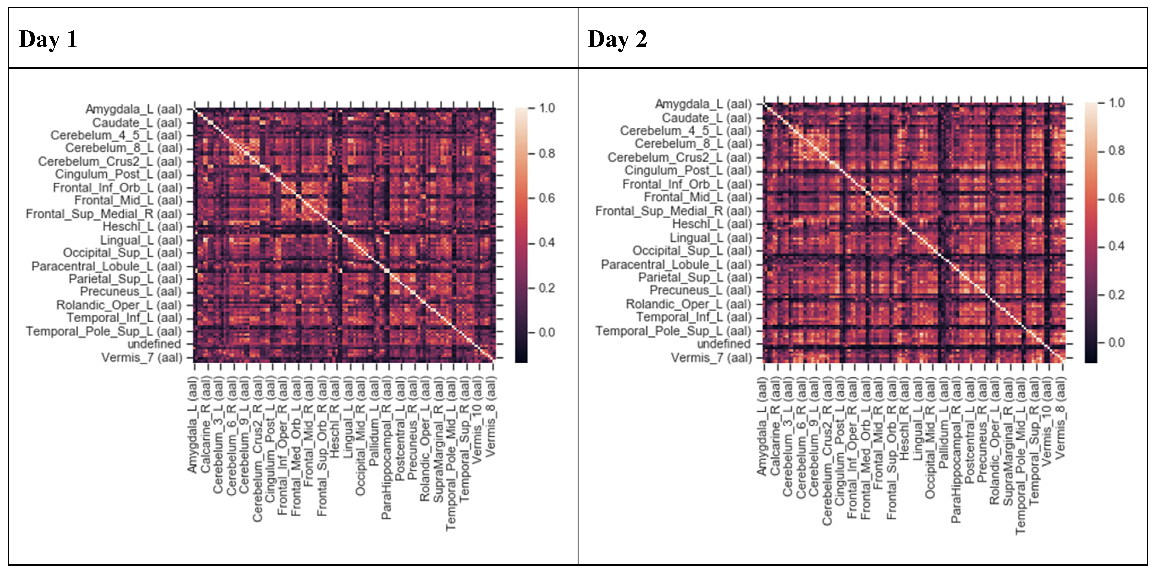
2.6. Feature Extraction
2.7. Feature Selection and Predictive Model Building
3. Results
3.1. Subjects
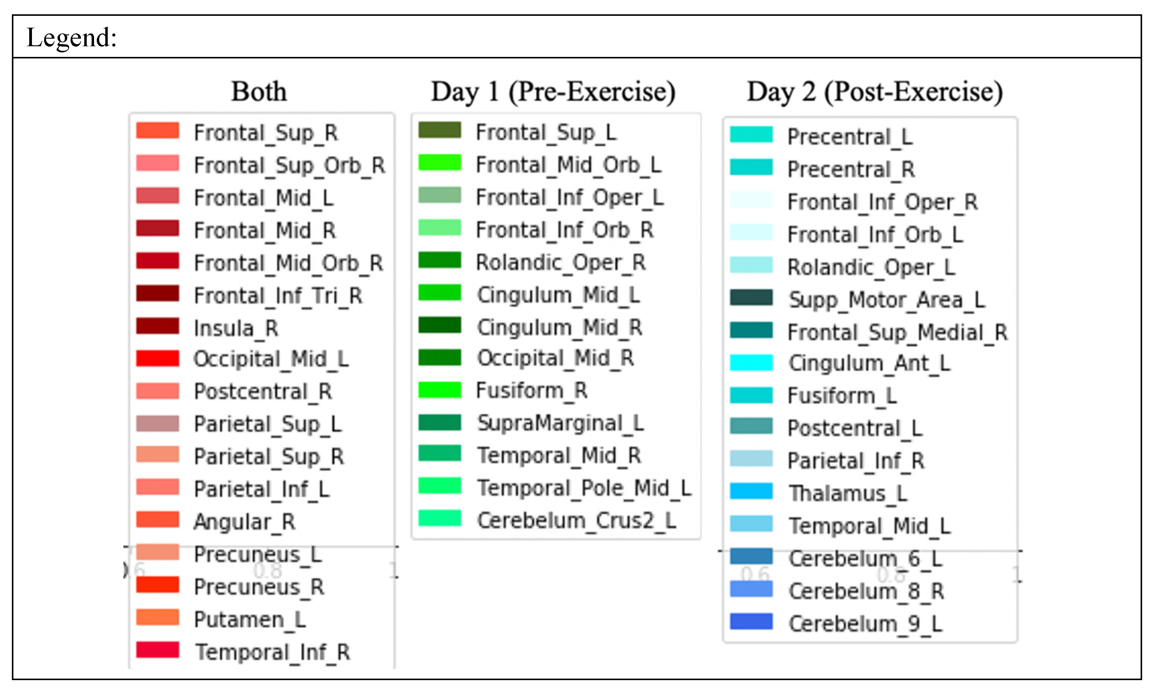
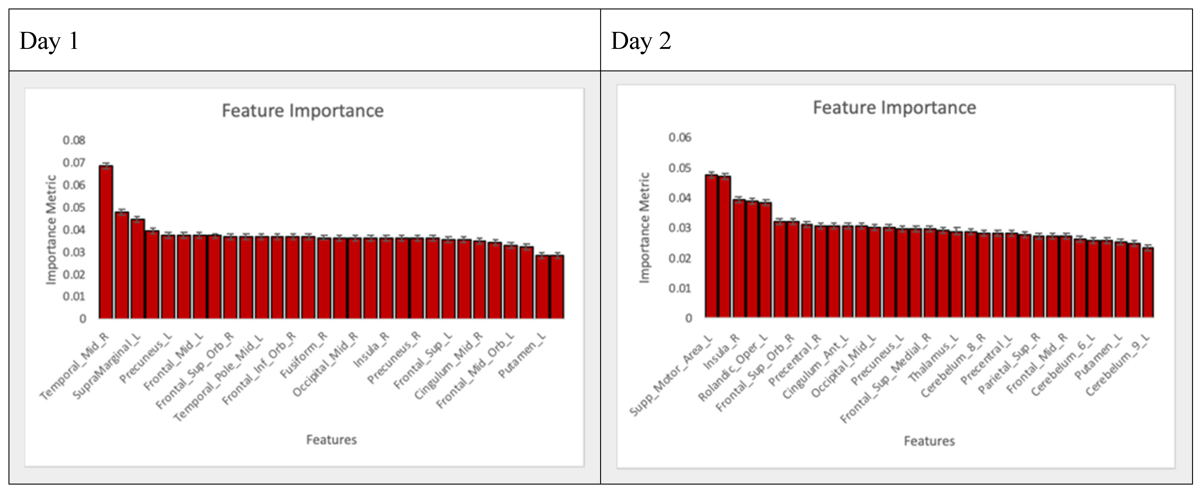
3.2. Feature Extraction
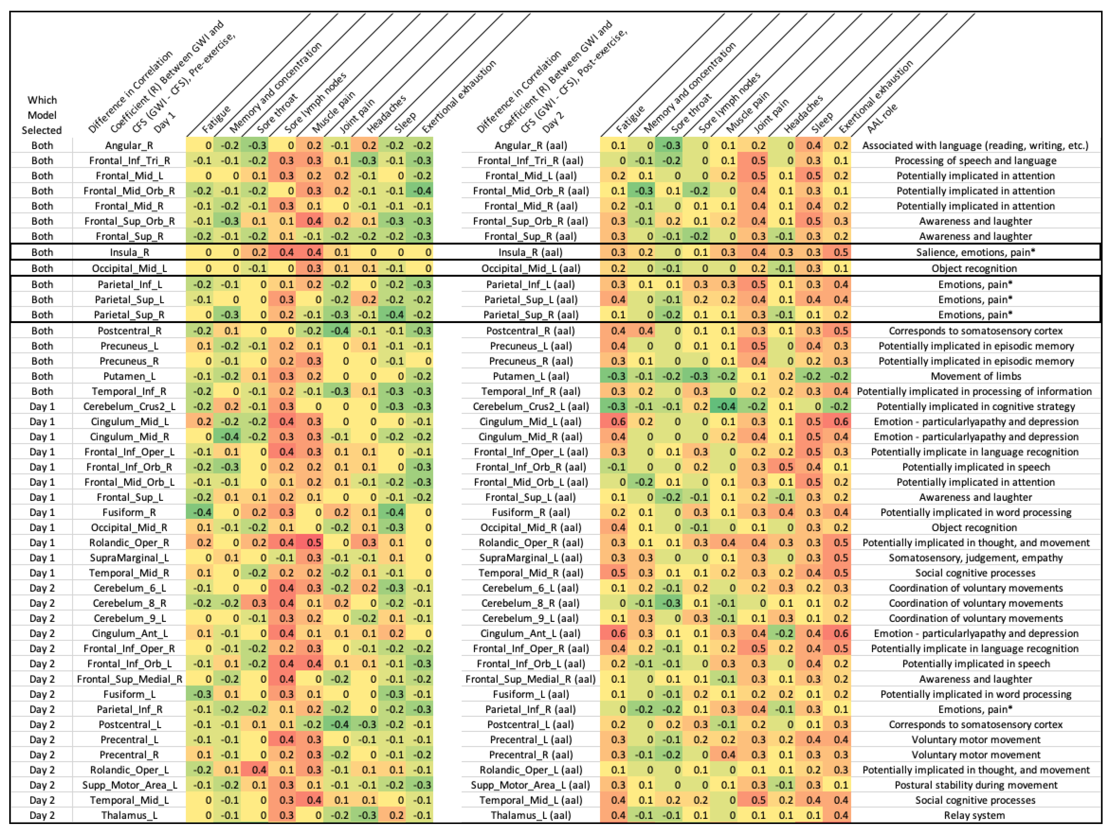
3.3. Feature Selection
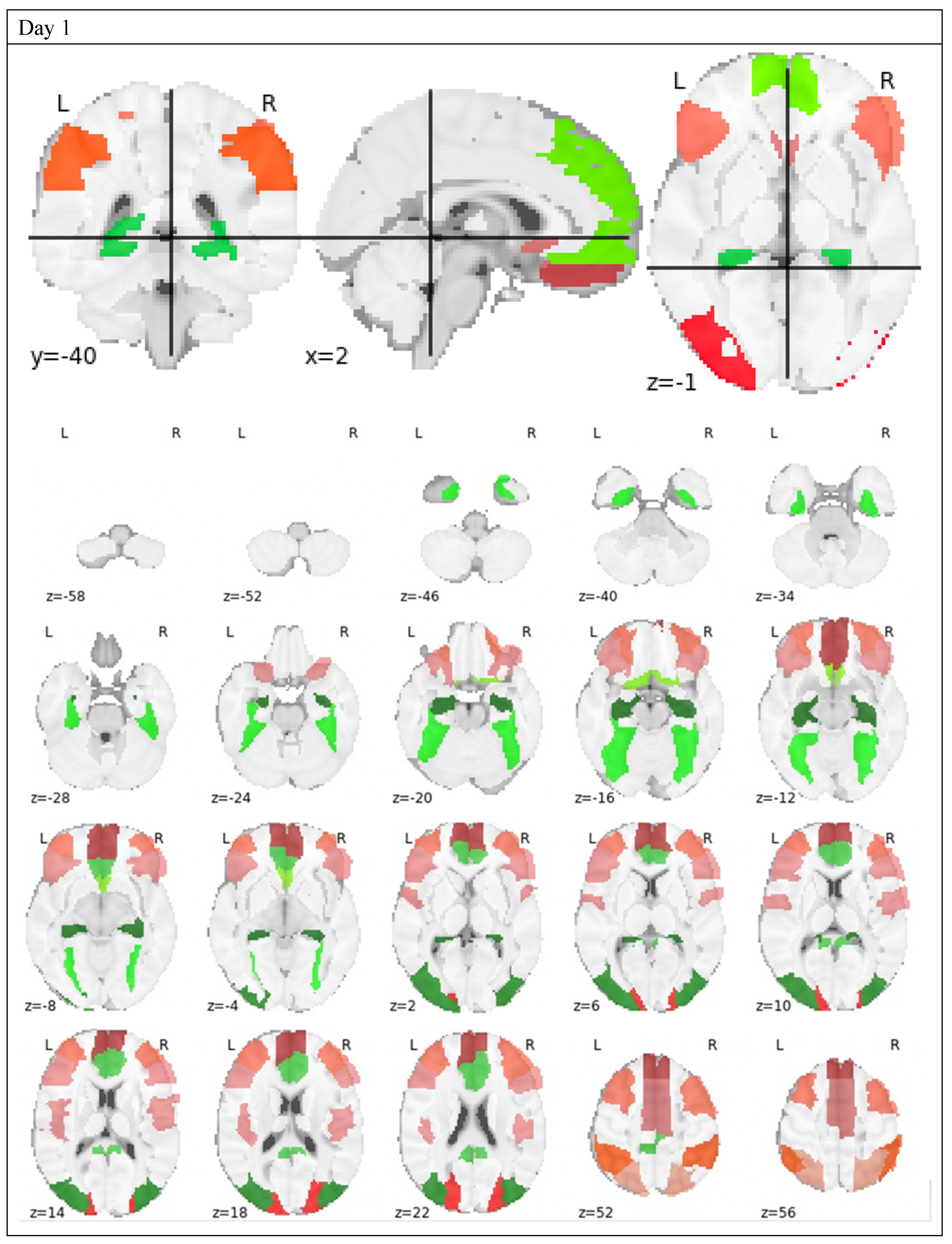
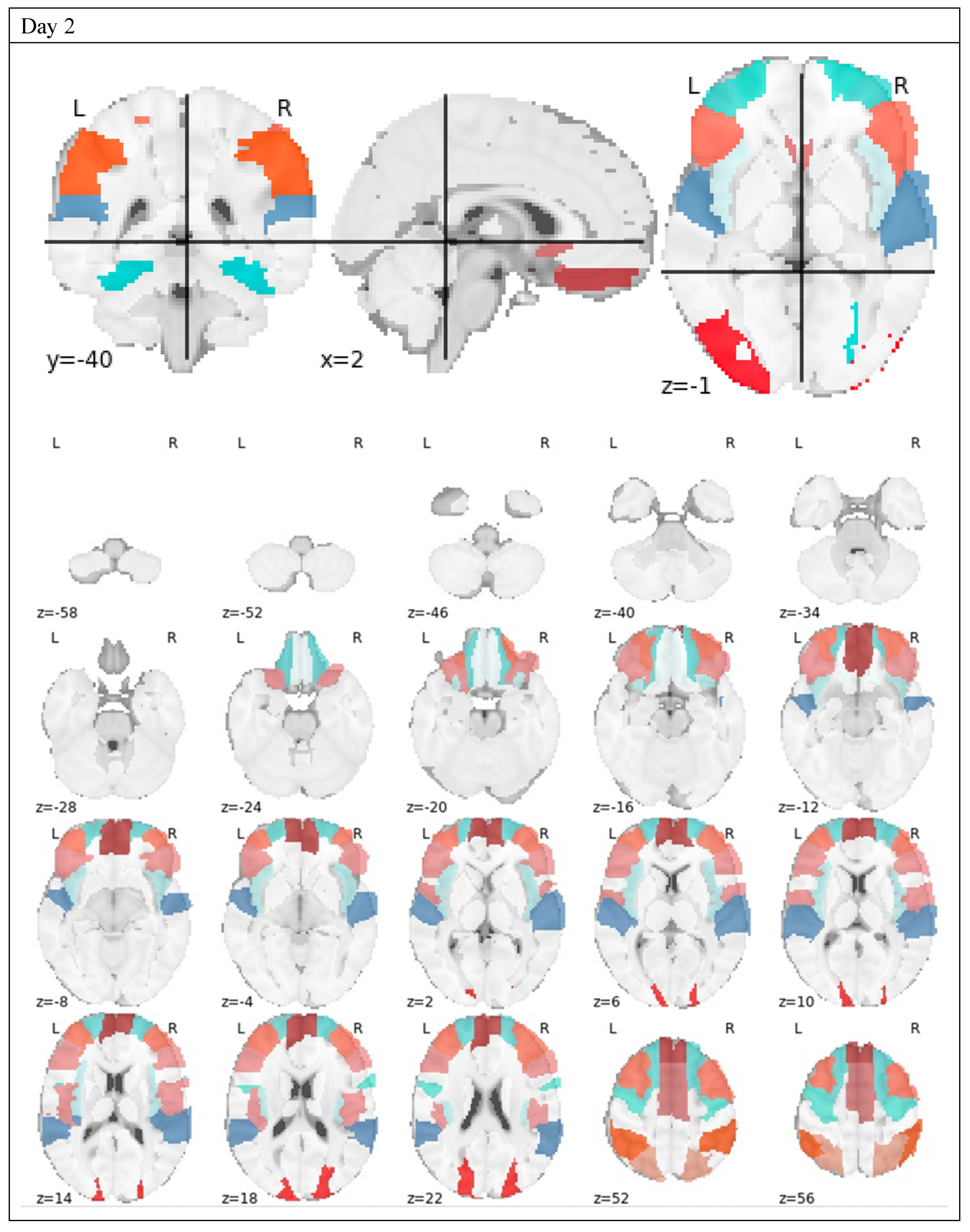
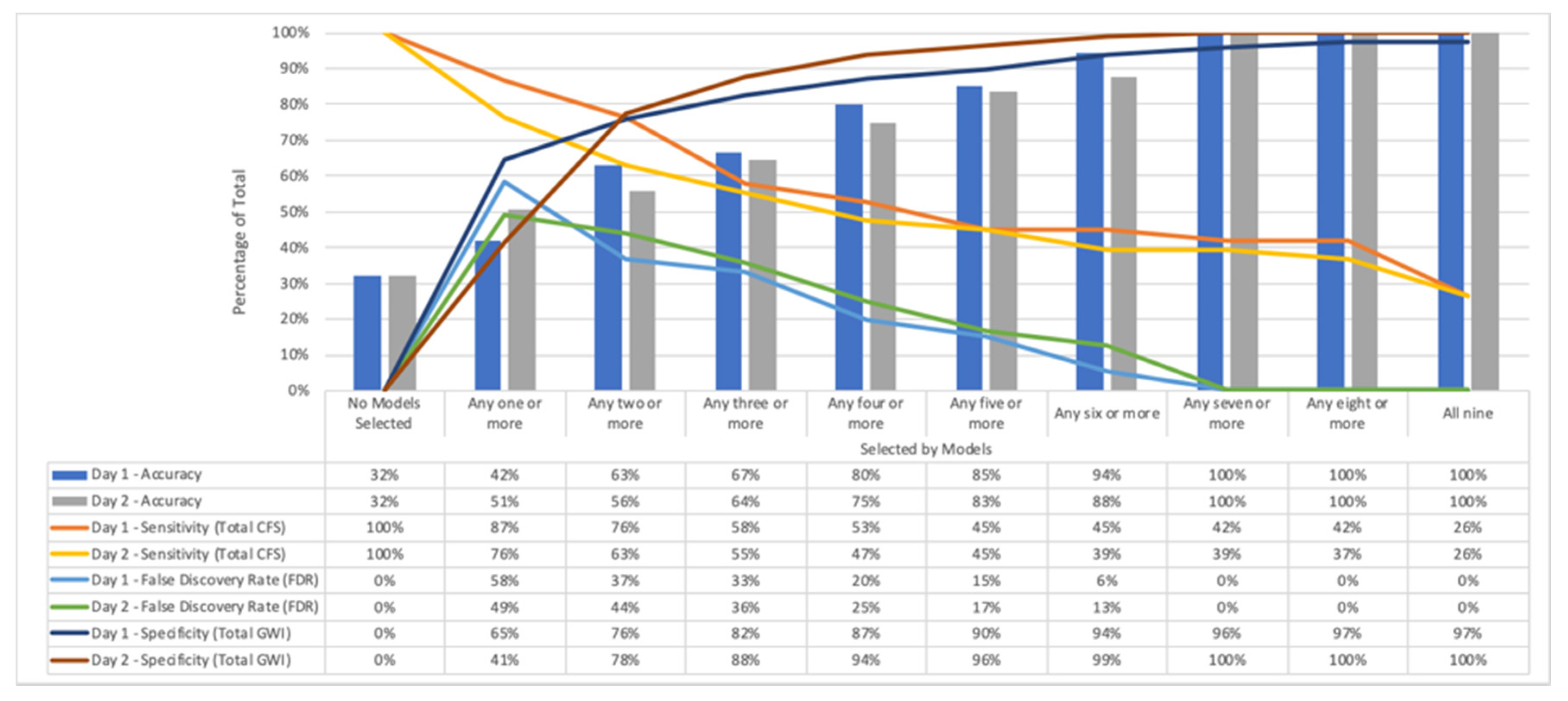
3.4. Model Results and Validation
4. Discussion
5. Conclusions
Supplementary Materials
Author Contributions
Funding
Acknowledgments
Conflicts of Interest
References
- Steele, L. Prevalence and patterns of Gulf War illness in Kansas veterans: Association of symptoms with characteristics of person, place, and time of military service. Am. J. Epidemiol. 2000, 152, 992–1002. [Google Scholar] [CrossRef]
- Centers for Disease Control and Prevention. Chronic Fatigue Syndrome. 26 May 2006. Available online: www.cdc.gov/cfs (accessed on 8 September 2018).
- Fukuda, K.; Straus, S.E.; Hickie, I.; Sharpe, M.C.; Dobbins, J.G.; Komaroff, A. The chronic fatigue syndrome: A comprehensive approach to its definition and study. International Chronic Fatigue Syndrome Study Group. Ann. Intern. Med. 1994, 121, 953–959. [Google Scholar] [CrossRef] [PubMed]
- Carruthers, B.M.; Jain, A.K.; de Meirleir, K.; Peterson, D.L.; Klimas, N.G.; Lerner, A.M.; Bested, A.C.; Florhenry, P.; Joshi, P.; Powles, A.C.P.; et al. Myalgic Encephalomyelitis/Chronic Fatigue Syndrome. J. Chronic Fatigue Syndr. 2003, 11, 7–115. [Google Scholar] [CrossRef]
- Committee on the Diagnostic Criteria for Myalgic Encephalomyelitis/Chronic Fatigue Syndrome; Board on the Health of Select Populations; Institute of Medicine. Beyond Myalgic Encephalomyelitis/Chronic Fatigue Syndrome: Redefining an Illness; National Academies Press: Washington, DC, USA, 2015. [Google Scholar]
- Steele, L.; Sastre, A.; Gerkovich, M.M.; Cook, M.R. Complex factors in the etiology of Gulf War illness: Wartime exposures and risk factors in veteran subgroups. Environ. Health Perspect. 2012, 120, 112–118. [Google Scholar] [CrossRef] [PubMed]
- Fukuda, K.; Nisenbaum, R.; Stewart, G.; Thompson, W.W.; Robin, L.; Washko, R.M.; Noah, D.L.; Barrett, D.H.; Randall, B.; Herwaldt, B.L.; et al. Chronic multisymptom illness affecting air force veterans of the gulf war. JAMA 1998, 280, 981–988. [Google Scholar] [CrossRef]
- Gronseth, G.S. Gulf War Syndrome: A Toxic Exposure? A Systematic Review. Neurol. Clin. 2005, 23, 523–540. [Google Scholar] [CrossRef]
- Pearce, J.M. The enigma of chronic fatigue. Eur. Neurol. 2006, 56, 31–36. [Google Scholar] [CrossRef]
- Pichot, P. La neurasthénie, hier et aujourd’hui [Neurasthenia, yesterday and today]. Encephale 1994, 20, 545–549. [Google Scholar]
- Rayhan, R.U.; Stevens, B.W.; Raksit, M.P.; Ripple, J.A.; Timbol, C.R.; Adewuyi, O.; Vanmeter, J.W.; Baraniuk, J.N. Exercise Challenge in Gulf War Illness Reveals Two Subgroups with Altered Brain Structure and Function. PLoS ONE 2013, 8, e63903. [Google Scholar] [CrossRef]
- Friston, K.J.; Holmes, A.P.; Worsley, K.J.; Poline, J.P.; Frith, C.D.; Frackowiak, R.S.J. Statistical parametric maps in functional imaging: A general linear approach. HBM 1995, 2, 189–210. [Google Scholar] [CrossRef]
- Mourao-Miranda, J.; Bokde, A.L.; Born, C.; Hampel, H.; Stetter, M. Classifying brain states and determining the discriminating activation patterns: Support Vector Machine on functional MRI data. Neuroimage 2005, 28, 980–995. [Google Scholar] [CrossRef]
- Pereira, F.; Mitchell, T.; Botvinick, M. Machine learning classifiers and fMRI: A tutorial overview. Neuroimage 2009, 45, S199–S209. [Google Scholar] [CrossRef] [PubMed]
- Ryali, S.; Supekar, K.; Abrams, D.A.; Menon, V. Sparse logistic regression for whole brain classification of fMRI data. NeuroImage 2010, 51, 752–764. [Google Scholar] [CrossRef]
- Cox, D.D.; Savoy, R.L. Functional magnetic resonance imaging (fMRI) “brain reading”: Detecting and classifying distributed patterns of fMRI activity in human visual cortex. Neuroimage 2003, 19, 261–270. [Google Scholar] [CrossRef]
- De Martino, F.; Valente, G.; Staeren, N.; Ashburner, J.; Goebel, R.; Formisano, E. Combining multivariate voxel selection and support vector machines for mapping and classification of fMRI spatial patterns. Neuroimage 2008, 43, 44–58. [Google Scholar] [CrossRef] [PubMed]
- Haynes, J.D.; Sakai, K.; Rees, G.; Gilbert, S.; Frith, C.; Passingham, R.E. Reading hidden intentions in the human brain. Curr. Biol. 2007, 17, 323–328. [Google Scholar] [CrossRef] [PubMed]
- Kriegeskorte, N.; Goebel, R.; Bandettini, P. Information-based functional brain mapping. Proc. Natl. Acad. Sci. USA 2006, 103, 3863–3868. [Google Scholar] [CrossRef] [PubMed]
- Okada, T.; Tanaka, M.; Kuratsune, H.; Watanabe, Y.; Sadato, N. Mechanisms underlying fatigue: A voxel-based morphometric study of chronic fatigue syndrome. BMC Neurol. 2004, 4, 14. [Google Scholar] [CrossRef] [PubMed]
- Lange, G.; Steffener, J.; Cook, D.B.; Bly, B.M.; Christodoulou, C.; Liu, W.; Deluca, J.; Natelson, B.H. Objective evidence of cognitive complaints in Chronic Fatigue Syndrome: A BOLD fMRI study of verbal working memory. Neuroimage 2005, 26, 513–524. [Google Scholar] [CrossRef]
- De Lange, F.P.; Kalkman, J.S.; Bleijenberg, G.; Hagoort, P.; van der Werf, S.P.; van der Meer, J.W.M.; Toni, I. Neural correlates of the chronic fatigue syndrome: An fMRI study [published online ahead of print July 7, 2004]. Brain 2004, 127, 1948–1957. [Google Scholar] [CrossRef]
- Washington, S.D.; Rayhan, R.U.; Garner, R.; Provenzano, D.; Zajur, K.; Addiego, F.M.; VanMeter, J.W.; Baraniuk, J.N. Exercise alters cerebellar and cortical activity related to working memory in phenotypes of Gulf War Illness. Brain Commun. 2020, 2, fcz039. [Google Scholar] [CrossRef] [PubMed]
- Provenzano, D.; Washington, S.D.; Baraniuk, J.N. A Machine Learning Approach to the Differentiation of Functional Magnetic Resonance Imaging Data of Chronic Fatigue Syndrome (CFS) From a Sedentary Control. Front. Comput. Neurosci. 2020, 14, 2. [Google Scholar] [CrossRef] [PubMed]
- Provenzano, D.; Washington, S.D.; Rao, Y.J.; Loew, M.; Baraniuk, J.N. Logistic Regression Algorithm Differentiates Gulf War Illness (GWI) Functional Magnetic Resonance Imaging (fMRI) Data from a Sedentary Control. Brain Sci. 2020, 10, 319. [Google Scholar] [CrossRef] [PubMed]
- Sen, B.; Borle, N.C.; Greiner, R.; Brown, M.R.G. A general prediction model for the detection of ADHD and Autism using structural and functional MRI. PLoS ONE 2018, 13, e0194856. [Google Scholar] [CrossRef]
- Opitz, D.; Maclin, R. Popular ensemble methods: An empirical study. J. Artif. Intell. Res. 1999, 11, 169–198. [Google Scholar] [CrossRef]
- Polikar, R. Ensemble based systems in decision making. IEEE Circuits Syst. Mag. 2006, 6, 21–45. [Google Scholar] [CrossRef]
- Rokach, L. Ensemble-based classifiers. Artif. Intell. Rev. 2010, 33, 1–39. [Google Scholar] [CrossRef]
- Breiman, L. Bagging Predictors. Mach. Learn. 1996, 24, 123–140. [Google Scholar] [CrossRef]
- Long, Z.; Huang, J.; Li, B.; Li, Z.; Li, Z.; Chen, H.; Jing, B. A Comparative Atlas-Based Recognition of Mild Cognitive Impairment with Voxel-Based Morphometry. Front. Neurosci. 2018, 12, 916. [Google Scholar] [CrossRef]
- Sill, J.; Takacs, G.; Mackey, L.; Lin, D. Feature-Weighted Linear Stacking. arXiv 2009, arXiv:0911.0460. Bibcode:2009arXiv0911.0460S. [Google Scholar]
- Bensusan, H.; Giraudcarrier, C. Discovering Task Neighbourhoods through Landmark Learning Performances (PDF). In Proceedings of the Principles of Data Mining and Knowledge Discovery, Lecture Notes in Computer Science, Lyon, France, 13–16 September 2000; pp. 325–330. [Google Scholar] [CrossRef]
- Breiman, L. Stacked regressions. Mach. Learn. 1996, 24, 49–64. [Google Scholar] [CrossRef]
- Nater, U.M.; Lin, J.S.; Maloney, E.M.; Jones, J.F.; Tian, H.; Boneva, R.S.; Raison, C.L.; Reeves, W.C.; Heim, C. Psychiatric comorbidity in persons with chronic fatigue syndrome identified from the Georgia population. Psychosom. Med. 2009, 71, 557–565. [Google Scholar] [CrossRef]
- Jones, J.F.; Lin, J.M.; Maloney, E.M.; Boneva, R.S.; Nater, U.M.; Unger, E.R.; Reeves, W.C. An evaluation of exclusionary medical/psychiatric conditions in the definition of chronic fatigue syndrome. BMC Med. 2009, 7, 57. [Google Scholar] [CrossRef] [PubMed]
- Rayhan, R.U.; Stevens, B.W.; Timbol, C.R.; Adewuyi, O.; Walitt, B.; Vanmeter, J.W.; Baraniuk, J.N. Increased brain white matter axial diffusivity associated with fatigue, pain and hyperalgesia in Gulf War illness. PLoS ONE 2013, 8, e58493. [Google Scholar] [CrossRef]
- Baraniuk, J.N.; El-Amin, S.; Corey, R.; Rayhan, R.; Timbol, C. Carnosine treatment for gulf war illness: A randomized controlled trial. Glob. J. Health Sci. 2013, 5, 69–81. [Google Scholar] [CrossRef]
- Clarke, T.; Jamieson, J.; Malone, P.; Rayhan, R.; Washington, S.; Van Meter, J.; Baraniuk, J. Connectivity differences between Gulf War Illness (GWI) phenotypes during a test of attention. PLoS ONE 2019. [Google Scholar] [CrossRef]
- Garner, R.S.; Rayhan, R.U.; Baraniuk, J.N. Verification of exercise-induced transient postural tachycardia phenotype in Gulf War Illness. Am. J. Transl. Res. 2018, 10, 3254–3264. [Google Scholar] [PubMed]
- Whitfield-Gabrieli, S.; Nieto-Castanon, A. Conn: A functional connectivity toolbox for correlated and anticorrelated brain networks. Brain 2012, 2, 125–141. [Google Scholar] [CrossRef] [PubMed]
- Mazziotta, J.C.; Toga, A.W.; Evans, A.; Fox, P.; Lancaster, J. A Probabilistic Atlas of the Human Brain: Theory and Rationale for Its Development: The International Consortium for Brain Mapping (ICBM). NeuroImage 1995, 2, 89–101. [Google Scholar] [CrossRef]
- SPM12. Available online: http://www.fil.ion.ucl.ac.uk/spm/software/spm12/ (accessed on 3 March 2020).
- XjView. Available online: http://www.alivelearn.net/xjview/ (accessed on 3 March 2020).
- Abbreviations and MNI Coordinates of AAL 27. Available online: https://figshare.com/articles/_Abbreviations_and_MNI_coordinates_of_AAL_/184981 (accessed on 3 March 2020).
- Kumar, T.K. Multicollinearity in Regression Analysis. Rev. Econ. Stat. 1975, 57, 365–366. [Google Scholar] [CrossRef]
- O’Brien, R.M. A Caution Regarding Rules of Thumb for Variance Inflation Factors. Qual. Quant. 2007, 41, 673. [Google Scholar] [CrossRef]
- Belsley, D. Conditioning Diagnostics: Collinearity and Weak Data in Regression; Wiley: New York, NY, USA, 1991; ISBN 0-471-52889-7. [Google Scholar]
- Farrar, D.E.; Glauber, R.R. Multicollinearity in Regression Analysis: The Problem Revisited. Rev. Econ. Stat. 1967, 49, 92–107. [Google Scholar] [CrossRef]
- O’Hagan, J.; McCabe, B. Tests for the Severity of Multicolinearity in Regression Analysis: A Comment. Rev. Econ. Stat. 1975, 57, 368–370. [Google Scholar] [CrossRef]
- Pedregosa, F.; Varoquaux, G.; Gramfort, A.; Michel, V.; Thirion, B.; Grisel, O.; Blondel, M.; Prettenhofer, P.; Weiss, R.; Dubourg, V.; et al. Scikit-learn: Machine Learning in Python. J. Mach. Learn. Res. 2011, 12, 2825–2830. [Google Scholar]
- Bonferroni, C.E. Teoria Statistica Delle Classi e Calcolo Delle Probabilità; Pubblicazioni del R Istituto Superiore di Scienze Economiche e Commerciali di Firenze; Springer: New York, NY, USA, 1936. [Google Scholar]
- Baraniuk, J.N.; Adewuyi, O.; Merck, S.J.; Ali, M.; Ravindran, M.K.; Timbol, C.R.; Rayhan, R.; Zheng, Y.; Le, U.; Esteitie, R.; et al. A Chronic Fatigue Syndrome (CFS) severity score based on case designation criteria. Am. J. Transl. Res. 2013, 5, 53–68. [Google Scholar]
- Ware, J.E., Jr.; Gandek, B. Overview of the SF-36 Health Survey and the International Quality of Life Assessment (IQOLA) Project. J. Clin. Epidemiol. 1998, 51, 903–912. [Google Scholar] [CrossRef]
- Padoa-Schioppa, C.; Conen, K.E. Orbitofrontal Cortex: A Neural Circuit for Economic Decisions. Neuron 2017, 96, 736–754. [Google Scholar] [CrossRef] [PubMed]


| Group | GWI | CFS |
|---|---|---|
| N | 80 | 38 |
| Age | 46.9 ± 7.8 | 47.74 ± 16.46 |
| BMI | 29.6 ± 5.6 | 26.20 ± 4.52 |
| Male | 59 (73.8%) | 10 (26.3%) † |
| White | 64 (80.0%) | 34 (89.4%) † |
| CFS Symptom Severity Scores *,† | ||
| Fatigue | 3.5 ± 0.7 | 3.4 ± 0.8 ** |
| Memory and concentration | 3.1 ± 0.8 | 2.9 ± 0.9 ** |
| Sore throat | 1.4 ± 1.2 | 1.0 ± 1.0 * |
| Sore lymph nodes | 1.5 ± 1.3 | 1.0 ± 1.1 * |
| Muscle pain | 3.1 ± 1.0 | 2.5 ± 1.3 ** |
| Joint pain | 3.2 ± 1.0 | 1.8 ± 1.4 * |
| Headaches | 2.7 ± 1.2 | 2.0 ± 1.3 * |
| Sleep | 3.5 ± 0.8 | 3.2 ± 0.9 ** |
| Exertional exhaustion | 3.3 ± 1.0 | 3.5 ± 0.8 ** |
| Day 1 (Pre-Submaximal Exercise) | Day 2 (Post-Submaximal Exercise) | ||||||
|---|---|---|---|---|---|---|---|
| Feature | Random Forest Importance | SVM (Linear Kernel) | Logistic Regression | Random Forest Importance | SVM (Linear Kernel) | Logistic Regression | |
| Observed in Both | Angular_R | −0.04 | 0.03 | 0.08 | −0.03 | 0.01 | 0.04 |
| Frontal_Inf_Tri_R | −0.03 | −0.01 | −0.02 | −0.04 | −0.06 | −0.2 | |
| Frontal_Mid_L | −0.04 | 0.01 | 0.04 | −0.02 | 0.01 | 0.06 | |
| Frontal_Mid_Orb_R | −0.03 | 0.04 | 0.18 | −0.03 | −0.02 | −0.08 | |
| Frontal_Mid_R | −0.03 | −0.01 | −0.02 | −0.03 | 0 | −0.02 | |
| Frontal_Sup_Orb_R | −0.03 | −0.18 | −0.59 | −0.02 | −0.01 | −0.1 | |
| Frontal_Sup_R | −0.03 | 0.02 | 0.05 | −0.03 | 0.04 | 0.16 | |
| Insula_R | −0.03 | 0.03 | 0.13 | −0.02 | 0.07 | 0.26 | |
| Occipital_Mid_L | −0.03 | −0.03 | −0.07 | −0.03 | −0.02 | −0.1 | |
| Parietal_Inf_L | −0.04 | 0 | −0.01 | −0.03 | −0.02 | −0.06 | |
| Parietal_Sup_L | −0.03 | 0.01 | 0.04 | −0.03 | −0.02 | −0.09 | |
| Parietal_Sup_R | −0.04 | −0.01 | −0.02 | −0.05 | −0.02 | −0.06 | |
| Postcentral_R | −0.03 | 0.05 | 0.13 | −0.03 | 0.05 | 0.21 | |
| Precuneus_L | −0.03 | 0.01 | 0.01 | −0.04 | −0.04 | −0.13 | |
| Precuneus_R | −0.03 | −0.01 | −0.05 | −0.04 | 0.01 | 0.04 | |
| Putamen_L | −0.03 | 0.2 | 0.81 | −0.03 | −0.02 | −0.08 | |
| Temporal_Inf_R | −0.03 | 0 | 0.03 | −0.03 | 0.01 | 0.07 | |
| Day 1 Only (Before Exercise) | Cerebellum_Crus2_L | −0.04 | 0.01 | 0.02 | |||
| Cingulum_Mid_L | −0.04 | 0.05 | 0.15 | ||||
| Cingulum_Mid_R | −0.04 | −0.08 | −0.28 | ||||
| Frontal_Inf_Oper_L | −0.04 | −0.02 | −0.08 | ||||
| Frontal_Inf_Orb_R | −0.04 | 0 | −0.02 | ||||
| Frontal_Mid_Orb_L | −0.04 | −0.13 | −0.44 | ||||
| Frontal_Sup_L | −0.03 | 0.02 | 0.06 | ||||
| Fusiform_R | −0.03 | 0 | −0.04 | ||||
| Occipital_Mid_R | −0.03 | −0.08 | −0.23 | ||||
| Rolandic_Oper_R | −0.03 | 0.01 | 0.14 | ||||
| SupraMarginal_L | −0.03 | −0.01 | −0.07 | ||||
| Temporal_Mid_R | −0.04 | 0.01 | 0 | ||||
| Temporal_Pole_Mid_L | −0.03 | 0.01 | 0.11 | ||||
| Day 2 Only (After Exercise) | Cerebellum_6_L | −0.03 | 0.08 | 0.32 | |||
| Cerebellum_8_R | −0.02 | 0.02 | 0.12 | ||||
| Cerebellum_9_L | −0.03 | 0.1 | 0.35 | ||||
| Cingulum_Ant_L | −0.02 | −0.02 | −0.03 | ||||
| Frontal_Inf_Oper_R | −0.03 | 0.02 | 0 | ||||
| Frontal_Inf_Orb_L | −0.02 | 0.08 | 0.3 | ||||
| Frontal_Sup_Medial_R | −0.03 | −0.16 | −0.59 | ||||
| Fusiform_L | −0.03 | −0.04 | −0.11 | ||||
| Parietal_Inf_R | −0.03 | −0.01 | −0.02 | ||||
| Postcentral_L | −0.04 | 0.06 | 0.23 | ||||
| Precentral_L | −0.03 | −0.02 | −0.09 | ||||
| Precentral_R | −0.03 | −0.03 | −0.08 | ||||
| Rolandic_Oper_L | −0.03 | −0.06 | −0.23 | ||||
| Supp_Motor_Area_L | −0.05 | 0.03 | 0.12 | ||||
| Temporal_Mid_L | −0.03 | 0.03 | 0.07 | ||||
| Thalamus_L | −0.04 | 0.02 | 0.08 | ||||
| Models | Day 1 (Pre-Submaximal Exercise) Accuracy | Day 2 (Post-Submaximal Exercise) Accuracy |
|---|---|---|
| K-Nearest Neighbors | 70% | 81% |
| Linear SVM | 70% | 77% |
| Decision Tree | 82% | 82% |
| Random Forest | 77% | 78% |
| AdaBoost | 69% | 81% |
| Naïve Bayes | 74% | 78% |
| Quadratic Discriminant Analysis (QDA) | 73% | 75% |
| Logistic Regression | 82% | 82% |
| Neural Net | 76% | 77% |
| Average | 75% ± 5% | 79% ± 2% |
© 2020 by the authors. Licensee MDPI, Basel, Switzerland. This article is an open access article distributed under the terms and conditions of the Creative Commons Attribution (CC BY) license (http://creativecommons.org/licenses/by/4.0/).
Share and Cite
Provenzano, D.; Washington, S.D.; Rao, Y.J.; Loew, M.; Baraniuk, J. Machine Learning Detects Pattern of Differences in Functional Magnetic Resonance Imaging (fMRI) Data between Chronic Fatigue Syndrome (CFS) and Gulf War Illness (GWI). Brain Sci. 2020, 10, 456. https://doi.org/10.3390/brainsci10070456
Provenzano D, Washington SD, Rao YJ, Loew M, Baraniuk J. Machine Learning Detects Pattern of Differences in Functional Magnetic Resonance Imaging (fMRI) Data between Chronic Fatigue Syndrome (CFS) and Gulf War Illness (GWI). Brain Sciences. 2020; 10(7):456. https://doi.org/10.3390/brainsci10070456
Chicago/Turabian StyleProvenzano, Destie, Stuart D. Washington, Yuan J. Rao, Murray Loew, and James Baraniuk. 2020. "Machine Learning Detects Pattern of Differences in Functional Magnetic Resonance Imaging (fMRI) Data between Chronic Fatigue Syndrome (CFS) and Gulf War Illness (GWI)" Brain Sciences 10, no. 7: 456. https://doi.org/10.3390/brainsci10070456
APA StyleProvenzano, D., Washington, S. D., Rao, Y. J., Loew, M., & Baraniuk, J. (2020). Machine Learning Detects Pattern of Differences in Functional Magnetic Resonance Imaging (fMRI) Data between Chronic Fatigue Syndrome (CFS) and Gulf War Illness (GWI). Brain Sciences, 10(7), 456. https://doi.org/10.3390/brainsci10070456