Effects of Background Sounds on Annoyance Reaction to Foreground Sounds in Psychoacoustic Experiments in the Laboratory: Limits and Consequences

Abstract

In a variety of applications, e.g., psychoacoustic experiments, virtual sound propagation demonstration, or synthesized noise production, noise samples are played back in laboratories. To simulate realistic scenes or to mask unwanted background sounds, it is sometimes preferable to add background ambient sounds to the noise. However, this can influence noise perception. It should be ensured that either background sounds do not affect, e.g., annoyance from foreground noise or that possible effects can be quantified. Two laboratory experiments are reported, in which effects of mixing background sounds to foreground helicopter samples were investigated. By means of partially balanced incomplete block designs, possible effects of three independent variables, i.e., helicopter’s sound exposure level, background type, and background sound pressure level were tested on the dependent variable annoyance, rated on the ICBEN 11-point numerical scale. The main predictor of annoyance was helicopter’s sound exposure level. Stimuli with eventful background sounds were found to be more annoying than those with less eventful background sounds. Furthermore, background type and level interacted significantly. For the major part of the background sound level range, increasing the background level was associated with increased or decreased annoyance for stimuli with eventful and less eventful background sounds, respectively.

1. Introduction

There are a variety of applications in the context of laboratory noise research or virtual acoustics for which background sounds are useful or, in many cases, necessary. The following is a non-exhaustive list in this regard.

It is possible to generate noise synthetically by means of emission synthesizers using physical and/or parametric approaches [1,2,3,4,5,6,7]. Adding recorded or synthesized (natural) background sounds to the noise samples helps to increase the degree of realism of the auralization. It is further possible to use propagation filters to simulate farther distances [4,8], in the case of which the recorded background sounds would also be sent to the target distance. Whereas in this case, only the source is aimed to be sent to the target distance, the background sounds are actually supposed to remain close to the observer. This problem can be solved with adding similar background sounds in the observer position [8].

When noise is recorded by a calibrated single microphone, as long as the exact momentary positions of the source and the observer are recorded as well, it would be possible to auralize the movement of the source on a multi-loudspeaker system. In this case, however, background sounds contained in the original recording (e.g., birds) would incorrectly move with the foreground noise from one loudspeaker to the other. Since the background sound should commonly be relatively static (with respect to its location), its movement with the noise could be extremely unrealistic and irritating. This might be solved by adding static background sounds to the moving noise which could partially mask the (moving) inherent background sound [8].

When virtual urban scenes are designed or virtual sound walks are simulated, they typically contain one or more background sound sources [9,10]. It is assumed that sounds of water features, birds, or natural vegetation would improve the virtual living (or urban) environment [11,12].

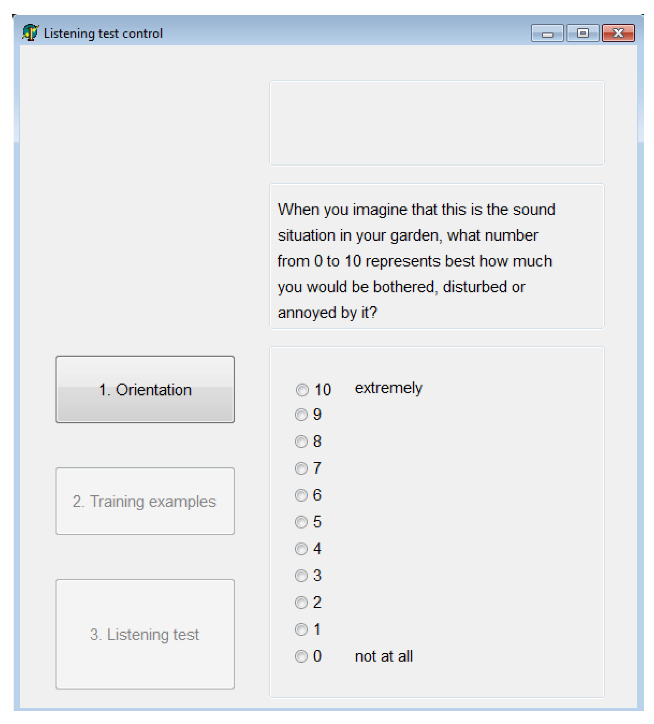
Generally, in a psychoacoustic experiment on acoustic comfort, sound pleasantness, or noise annoyance, stimuli are typically played back successively (i.e., one after the other). While the subjects are sitting in a lab, it is asked to imagine they would be sitting in an office, in the garden, in a wind park, at a street corner, or in other scenarios. Thereby, typically no sound of the imaginary environment—but rather silence—exists in-between the stimuli. It would be much more realistic to have a background sound present in the room for the whole duration of an experiment, from which each stimulus then arises into the foreground.

Furthermore, it should be mentioned that, although noise recordings are ideally carried out carefully such that they are free of dominant background sounds, still some sort of background sounds are present in any natural or everyday environment. Hence, the recorded foreground sound samples also contain some background sounds. In psychoacoustic experiments on acoustic comfort, pleasantness, or noise annoyance this introduces a possible source of error or bias, which should be controlled for.

The examples given above show the relevance and importance of background sounds in virtual audio and psychoacoustic applications. Whereas these examples justify the vast usage of background sounds in the respective contexts and for particular reasons, only a few studies investigated the effects they could have on the perception of the respective scenes.

A series of studies reported that background sounds in presence of noise sources might improve the acoustic quality of the urban soundscape [12,13,14,15]. For example, natural water features in urban environments were reported to reduce the loudness of road traffic noise [14,15] and of wind turbines [13]. They were further reported to reduce annoyance from the road traffic or wind turbines [12,13].

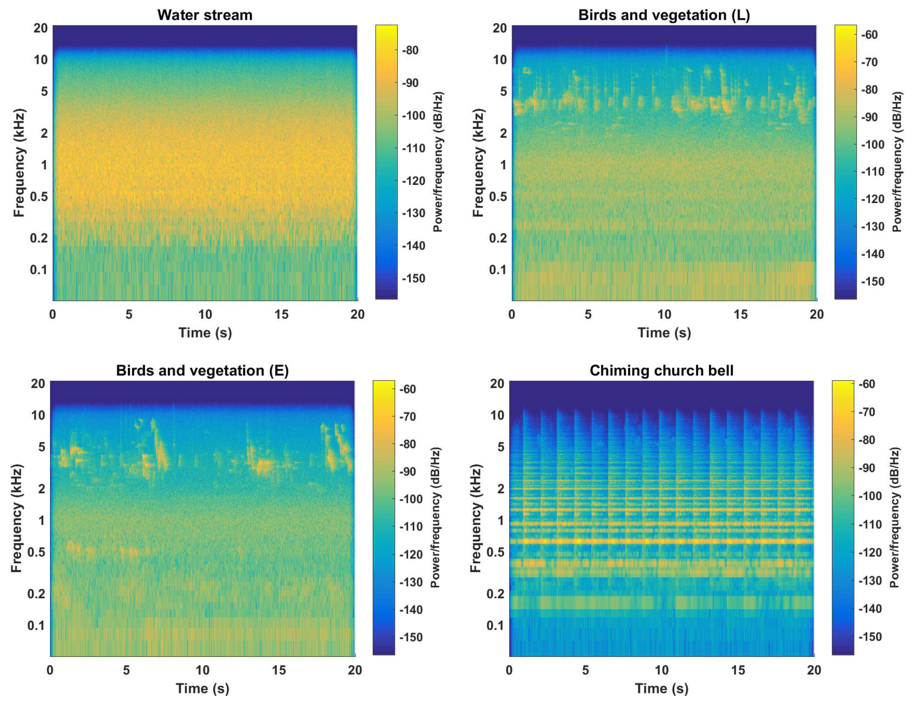
Bolin et al. [13] and Nilsson et al. [14] reported that auditory masking effects [16,17] of the natural background sounds on the noise could be exploited to improve the quality of the urban soundscape. For this, however, the level of a background sound must be comparable or higher than the level of the noise [16,17,18,19], in the case of which it might be incorrect to label them as “background” sounds. Nevertheless, because of its temporal variation, a background sound of singing birds was found to be a less effective masker than broadband natural sounds, such as a water stream (i.e., brook), deciduous vegetation, and coastal breaking waves [13]. On the other hand, bird sounds were found to improve pleasantness more strongly than water features [15]. Furthermore, Jeon et al. [12] reported that among nine different background sounds, “water stream” and “waves of lake” were found to be more preferable than other sounds to be used as mixed background sounds for road traffic noise as well as for construction noise.

De Coensel et al. [15] argued that not only the auditory masking, but also other perceptual processes, such as auditory attention, might affect the perception of noise in a mixture of noise and background sounds. Thereby it is assumed that, e.g., differences in the temporal structure of sounds are associated with different degrees of attention to them.

Yang et al. [20] suggested that values of psychoacoustic parameters fluctuation strength [16,21], sharpness [16,22], and loudness [16,23] were the three key indicators for characterization of sounds in soundscape. It can be hence summarized that not only different background sources (water, birds, vegetation, etc.) might influence the perception of the noise differently, but also the temporal structure [13,24], spectral structure [13,18,19], and the level [12,13,14,25] of the background sound could be important parameters for the altered perception of the noise. In accordance with that, Aletta et al. [26] suggested a holistic approach when categorizing the soundscape, considering the physical spectro-temporal characteristics, as well as the type and the meaning (i.e., the semantic content) of sounds.

With that background, this paper investigates possible effects of background sounds of different types and levels on the perceived annoyance of foreground noise. In particular, sounds of landing helicopters were used as an exemplary noise source. Unlike studies which investigated relatively high-level background sounds—partially masking the noise—in order to improve the urban soundscape [12,13,14], the study presented here focused on the usage of background sounds in psychoacoustic experiments and in virtual acoustic applications. Section 2 of this paper introduces briefly the experimental concept. Experimental design and setup follow in Section 3. Experiments 1 and 2 and their results are presented in Section 4 and Section 5, respectively. After a discussion of the outcomes in Section 6, Section 7 will conclude the paper.

2. Experimental Concept

Acute annoyance reactions to helicopter noise were investigated under laboratory conditions. The observed annoyance ratings correspond to “short-term annoyance” [27] or “psychoacoustic annoyance” [16], similar to the reported laboratory experiments by Schäffer et al. [28] and Taghipour et al. [8]. The term “short-term” refers to the time period during and after an acoustic stimulus’ playback and before the next stimulus is presented [9].

To investigate differences in short-term annoyance, stimuli were generated from field recordings (see Taghipour et al. [8]) of helicopter landings and from background ambient sounds. In both experiments presented here, three design parameters, i.e., two continuous variables, flight event’s A-weighted sound exposure level, ${\mathit{L}}_{\mathbf{AE},\mathbf{F}}$, and background sound’s A-weighted equivalent continuous sound pressure level, ${\mathit{L}}_{\mathbf{Aeq},\mathbf{B}}$, as well as the categorical variable background sound type (i.e., eventful vs. less eventful) were systematically varied to study their individual and combined associations with short-term annoyance ratings.

To avoid confusions between the foreground sound (i.e., the helicopter noise) and the ambient background sound, in this article, “noise” and “sound” are repeatedly used for these two categories of sounds, respectively. However, it should be noted that, in general, sounds are not to be labeled or prejudged as “noise” per se. It is rather for each individual observer to judge subjectively whether they perceive a sound as noise. Pleasantness or unpleasantness (including declaring a sound as “noise”) is not a definitive, but a (subjectively) perceived quality of sound, which can only be interpreted in the context under investigation [9,29].

The choice of landing helicopters as foreground noise was rather exemplary. A number of takeoffs and landings of civil helicopters and propeller-driven aircraft was available, which were calibrated, analyzed and already tested with regards to the perceived annoyance [8]. In order to avoid possible variations due to the type of aircraft (helicopter vs. propeller-driven aircraft) and procedure (takeoff vs. landing), only landing helicopters were chosen for this study. Whereas the ecological validity or plausibility of this particular noise situation is supported by landing civil helicopters in everyday life for medical, rescue, special transport, or sport (hobby) purposes, it should be noted that usage of other types of foreground noise samples (e.g., road traffic) might exhibit higher ecological validity [30]. Similar experiments are planned with other noise sources.

3. Experimental Design and Setup

3.1. Listening Test Facility

The two experiments presented here were conducted in AuraLab, a listening test facility of the Empa (Swiss Federal Laboratories for Materials Science and Technology), which has a separate listening and control room allowing for audio–visual supervision to comply with ethical requirements [8,9].

AuraLab satisfies room acoustical requirements for high-quality audio reproduction in terms of its background noise and reverberation time. The 3D immersive sound system with 15 loudspeakers (KH 120 A, Georg Neumann GmbH, Berlin, Germany) in a hemispherical arrangement and two subwoofers (KH 805, Georg Neumann GmbH, Berlin, Germany) is controlled by a digital signal processor [8]. The stimuli of the experiments were played back through one loudspeaker at a distance of 2 m from the listening spot and 0° elevation (subject’s ear level) as well as both subwoofers. The carpeted floor was covered with additional absorbers.

3.2. Stimuli Preparation

3.2.1. Recordings

The helicopter noise samples originated from field recordings of helicopter landings at Grenchen Airport, Switzerland (ICAO code: LSZG) [8]. Single-channel audio recordings were performed by means of a series of microphones (B&K 4188, Brül and Kjær, Naerum, Denmark) and (Nor 1227, Norsonic AS, Tranby, Norway) placed 4 m above the ground in the eastern side of the airport, on the left and right sides of the extension of the runway [8]. The six recordings selected for this study were from helicopter types A109, A119, AS35, and EC20, all of which are categorized as light-weight civil helicopters (weight: 1.7–3.2 tons). Helicopter recordings were done at the sampling frequency of 44.1 kHz and with 16 bit depth.

Single-channel recordings of ambient sound were done by means of a microphone (B&K 4006, Brül and Kjær, Naerum, Denmark) placed 2 m above the ground in and around the city of Dübendorf, Switzerland. Background sound recordings were carried out at the sampling frequency of 48 kHz and with 24 bit depth.

3.2.2. Signal Processing and Mixing

As mentioned above, six recordings of landing helicopters were chosen for the psychoacoustic experiments reported here. Furthermore, four background sound extracts were selected: two sounds with dominant events (i.e., a chiming church bell and singing birds) and two sounds with less dominant events (i.e., water stream and birds). Eventfulness in this context refers to a series of single dominant events with relatively high energy which arise from a rather low level background. Less eventful sounds are, on the contrary, sounds whose momentary sound pressure level do not vary extensively from their A-weighted equivalent continuous sound pressure level, $L_{\mathrm{Aeq},\mathrm{B}}$ [31]. The categorization of background sounds into eventful or less eventful was carried out by (qualitative) subjective evaluations by the experimenters and another environmental acoustician, as well as by objective differentiation based on signals’ intermittency ratio (IR) [31] and “$L_{10}-L_{90}$”. A series of sound temporal dynamics measures is listed in

Table 1. Information about the background sounds at the exemplary $L_{\mathrm{Aeq},\mathrm{B}}$ of 41 dB(A). For the calculation of intermittency ratio (IR), C is the dB-offset (i.e., the dB difference to $L_{\mathrm{Aeq},\mathrm{B}}$) beyond which events were counted [31].

Sound	Category	IR (%), $\mathit{C}=3$ dB	IR (%), $\mathit{C}=5$ dB	${\mathit{L}}_{\mathbf{AF},\mathbf{B},10}-{\mathit{L}}_{\mathbf{AF},\mathbf{B},90}$ (dB)
Water stream	L	58.7	38.7	0.8
Birds (and vegetation) L	L	62.3	48.6	5.3
Birds (and vegetation) E	E	77.3	70.9	13.5
Chiming church bell	E	67.9	55.2	8.8

to characterize the amount of single events in the signals. Furthermore, Figure 1 shows A-weighted spectrograms of the background sound signals.

The signals underwent the following processing steps to prepare them for playback in AuraLab. Most of the processing—beside bass management—was carried out with MATLAB R2016b (MathWorks, Natick, USA). In a first stage of processing, the recordings were calibrated, high-pass filtered ($f_c=20$ Hz), and low-pass filtered ($f_c=10$ kHz) to attenuate irrelevant noise (e.g., microphone inherent noise).

The duration of each stimulus was set to 20 s. While background signals were available at a sampling rate of 48 kHz, helicopter signals were upsampled from 44.1 to 48 kHz, which is a requirement of the playback system in AuraLab. The output (mixed) signals were of 16 bit depth.

Background and helicopter signals were faded in and out by squared cosine ramps of 0.5 and 4 s, respectively. That is, whereas the background sound was planned to be present during the stimulus duration of 20 s, the helicopter sound was supposed to be arising from and fading out into the background sound. The cuts for the helicopter signals were carried out (level-)symmetrical around their maximum A-weighted noise level $L_{\mathrm{ASmax},\mathrm{F}}$; i.e., in the range from $L_{\min }$ to $L_{\mathrm{ASmax},\mathrm{F}}$, whereby the exact value of $L_{\min }$ (i.e., a specific minimum level on the $L_{\mathrm{AS}}$ curve) varied for different flight events, corresponding to a (windowed) signal duration of 20 s. The sound pressure level of the helicopter noise signals and the background signals were modified to reach the target levels. That is, helicopter signals were attenuated and set to the target $L_{\mathrm{AE},\mathrm{F}}$. Furthermore, background signals were either attenuated or amplified to scale them to the target $L_{\mathrm{Aeq},\mathrm{B}}$.

It should be noted that not all stimuli were mixed. For comparison and as a baseline, the six helicopter samples were also prepared as single flight event stimuli of the target sound exposure levels of experiments 1 (six levels) and 2 (three levels), without any additional background sounds.

3.3. Experimental Sessions

The two experiments were conducted as focused listening tests with repeated measures and a partially balanced incomplete block design (PBIBD) [32]. Thereby each block was only assigned to one subject, only included a subset of the stimuli, and was therefore incomplete. Partially balanced means that all stimuli of an experiment were offered in an approximately equal number of blocks and, hence, were rated for an approximately equal number of times. Furthermore, an effort was made to partially balance every single parameter of the design for every single block/subject; i.e., for example, all the helicopter events were tested for an approximately equal number of times by each subject.

The experiment was carried out individually for each subject. After reading the study information and signing a consent form to participate, the subjects answered the first part of the questionnaire about their hearing and well-being. They were then introduced to the listening test and the test software which guided them throughout the test. Subjects rated their perceived annoyance they associated with each stimulus during or directly after its playback. After the listening test, the subjects filled out the remaining part of the questionnaire about their demographic data.

3.4. Listening Test Software and the Annoyance Scale

Figure 2 shows the experimental software’s graphical user interface (GUI). The software guided the subjects through the test and recorded their annoyance ratings. The subjects listened to a few orienting and a few training sounds before starting the main listening test. The stimuli were presented in a random order for each subject. They were played back once only, with a 1.5-s break between stimuli after each complete playback.

As shown in Figure 2, short-term annoyance was rated on the ICBEN 11-point numerical scale [33]. Thereby, the following (modified) question was asked for every stimulus: “when you imagine that this is the sound situation in your garden, what number from 0 to 10 represents best how much you would be bothered, disturbed or annoyed by it?”

3.5. Statistical Analysis

Statistical analysis was carried out with IBM SPSS Statistics, version 25 (IBM Corporation, Armonk, USA). Tested effects were considered significant if the observed data’s probability, p, of occurrence under the null hypothesis was ≤0.05.

Associations of design variables ($L_{\mathrm{AE},\mathrm{F}}$, $L_{\mathrm{Aeq},\mathrm{B}}$, and background type) with annoyance were analyzed by means of linear mixed effects models [34], combining fixed effects of categorical variable background type, covariates $L_{\mathrm{AE},\mathrm{F}}$, $L_{\mathrm{Aeq},\mathrm{B}}$, playback number, subjects’ random effects, and their interactions to predict dependent variables annoyance ratings. It should be noted that, for the statistical analysis, the variable background type was coded with three levels of “no background”, “eventful (E)”, and “less eventful (L)”, as the experimental hypothesis mainly focused on the eventfulness of the background.

Several models of different degrees of complexity were established. The models were compared using the Akaike information criterion (AIC) [35] and Bayesian information criterion (BIC) [36], where the model with the lowest AIC/BIC was preferred. Non-significant variables and interactions were excluded from the final models that will be presented later in this paper.

4. Experiment 1

Experiment 1 focused on the scenario in which the level of the background sound was reasonably low (i.e., compared to the level of the foreground helicopter noise). That is, mixed signal sound levels were not to be considerably higher than flight events’ sound levels:

• $L_{\mathrm{AE},\mathrm{S}}-L_{\mathrm{AE},\mathrm{F}}$ < 1 dB(A), whereby S stands for the (mixed) signal;
• $L_{\mathrm{ASmax},\mathrm{S}}-L_{\mathrm{ASmax},\mathrm{F}}$ < 1 dB(A);
• $L_{\mathrm{Aeq},\mathrm{S}}-L_{\mathrm{Aeq},\mathrm{F}}$ < 1 dB(A).

4.1. Method

4.1.1. Experimental Design

Three design variables—i.e., independent variables—were considered in the design of experiment 1: $L_{\mathrm{AE},\mathrm{F}}$ (six levels), $L_{\mathrm{Aeq},\mathrm{B}}$ (four levels), and background type (five levels). The partially balanced incomplete block design consisted of 32 blocks (i.e., subjects), each containing 40 stimuli.

Flight events’ $L_{\mathrm{AE},\mathrm{F}}$ were set to 68, 70, 72, 74, 76 or 78 dB(A). Background sounds’ $L_{\mathrm{Aeq},\mathrm{B}}$ were set to 6 (i.e., background level of AuraLab in case of “no background sound”), 34, 41, or 48 dB(A). Four background sounds were used which were either eventful, E, or less eventful, L: water stream (L), birds and vegetation (L), birds and vegetation (E), and church bell (E). An additional category was coded as “no background” when no background sound was available in the corresponding stimulus.

4.1.2. Stimuli

Based on the combination of six flight events (or levels, $L_{\mathrm{AE},\mathrm{F}}$), four $L_{\mathrm{Aeq},\mathrm{B}}$—i.e., 3 + 1 (Auralab background level)—, and five background types—i.e., 4 + 1 (no background sound)—, a total number of 78 stimuli were prepared for this experiment:

$$6\times 3\times 4+6(\mathrm{stimuli}\mathrm{without}\mathrm{background}\mathrm{sounds})=78.$$

Figure 3 shows $L_{\mathrm{AS},\mathrm{F}}$ as a function of time for the six flight events (without any mixed background sounds) used in experiment 1. A-weighted sound exposure levels of the stimuli (i.e., mixed flight and background), $L_{\mathrm{AE},\mathrm{S}}$, were between 68.0 to 78.1 dB(A) (mean $L_{\mathrm{AE},\mathrm{S}}=73.1$ dB(A)). Furthermore, $20\le L_{\mathrm{AE},\mathrm{F}}-L_{\mathrm{Aeq},\mathrm{B}}\le 72$ dB(A) and $0.0\le L_{\mathrm{AE},\mathrm{S}}-L_{\mathrm{AE},\mathrm{F}}\le 0.8$ dB(A).

4.1.3. Subjects

Thirty-two subjects (13 females and 19 males) participated in the main experiment. All subjects declared to have normal hearing (self judgement) and to feel well. They were aged between 21 and 50 yr (median 27.5 yr).

4.2. Results

In total, 1280 annoyance ratings were collected (32 subjects × 40 stimuli), each of which was assigned to a particular subject and a specific stimulus (of the total 78 stimuli). The results of experiment 1 are illustrated in Figure 4.

The following simple linear mixed effects model was found to be effective to predict annoyance:

$$y_{ik}=\mu +{\tau }_{\mathrm{B},i}+\beta ·L_{\mathrm{AE},\mathrm{F}}+\theta ·S_{ik}+u_k+{ϵ}_{ik}.$$

(1)

In Equation (1), $y_{ik}$ is the dependent variable annoyance, predicted for each background type and subject at different helicopter sound exposure levels and playback number. $\mu$ is the overall grand mean and ${\tau }_{\mathrm{B},i}$ denotes the categorical variables background type (three levels: $i=1,2,3$). Parameters $\beta$ and $\theta$ are regression coefficients for $L_{\mathrm{AE},\mathrm{F}}$ and $S_{ik}$, respectively. The (unstructured) random effect term $u_k$ is subjects’ random intercept—for $k=1$, …, 32. Finally, the error term ${ϵ}_{ik}$ is the random deviation between observed and expected values of $y_{ik}$. Model coefficients are listed in

Table 2. Experiment 1, model 1: model coefficients (Coeff.), their 95% confidence interval (CI), and probabilities (p) of the linear mixed effects model for annoyance. The parameters and symbols are explained in Equation (1).

Parameter	Symbol	Coeff.	95% CI	p
Intercept	$\mu$	−25.173	[−26.867;−23.479]	0.00
Background type	${\tau }_{\mathrm{B},i}$ = No	$0{}^a$
	${\tau }_{\mathrm{B},i}$ = L	0.063	[−0.225;0.350]	0.67
	${\tau }_{\mathrm{B},j}$ = E	0.280	[−0.006;0.567]	0.06
$L_{\mathrm{AE},\mathrm{F}}$	$\beta$	0.414	[0.392;0.435]	0.00
Playback No.	$\theta$	0.017	[0.011;0.024]	0.00

${}^a$ Redundant coefficients are set to zero.

.

The main predictor of annoyance was flight event’s sound exposure level, $L_{\mathrm{AE},\mathrm{F}}$ (p < 0.001). Annoyance increased with increasing $L_{\mathrm{AE},\mathrm{F}}$. Background type was a further significant predictor of annoyance (p < 0.05). Whereas no significant difference was found between average annoyance ratings for stimuli without background sounds and those with less eventful background sounds, stimuli containing eventful background sounds were found to be more annoying on average than the other two categories. Furthermore, annoyance increased slightly, however significantly, with the playback number (p < 0.001).

A second more complex linear mixed effects model was found to be optimal to predict annoyance:

$$y_{ik}=\mu +{\tau }_{\mathrm{B},i}+\beta ·L_{\mathrm{AE},\mathrm{F}}+\gamma ·L_{\mathrm{Aeq},\mathrm{B}}+\theta ·S_{ik}+{\gamma }_{\mathrm{B},i}·L_{\mathrm{Aeq},\mathrm{B}}+u_k+{ϵ}_{ik}.$$

(2)

In Equation (2), $y_{ik}$, $\mu$, ${\tau }_{\mathrm{B},i}$, $\beta$, $\theta$, $u_k$, and ${ϵ}_{ik}$ are the same parameters as in Equation (1). $\gamma$ is the regression coefficient for $L_{\mathrm{Aeq},\mathrm{B}}$ and ${\gamma }_{\mathrm{B},i}$ represents interaction between background type and background level $L_{\mathrm{Aeq},\mathrm{B}}$. Model coefficients are listed in

Table 3. Experiment 1, model 2: model coefficients (Coeff.), their 95% CI, and probabilities (p) of the linear mixed effects model for annoyance. The parameters and symbols are explained in Equation (2).

Parameter	Symbol	Coeff.	95% CI	p
Intercept	$\mu$	−25.056	[−26.754;−23.359]	0.00
Background type	${\tau }_{\mathrm{B},i}$ = No	$0{}^a$
	${\tau }_{\mathrm{B},i}$ = L	0.642	[−0.083;1.366]	0.08
	${\tau }_{\mathrm{B},j}$ = E	−0.353	[−1.191;0.485]	0.41
$L_{\mathrm{AE},\mathrm{F}}$	$\beta$	0.413	[0.392;0.435]	0.00
$L_{\mathrm{Aeq},\mathrm{B}}$	$\gamma$	−0.017	[−0.036;0.002]	0.09
Playback no.	$\theta$	0.017	[0.011;0.024]	0.00
Type $\times L_{\mathrm{Aeq},\mathrm{B}}$	${\gamma }_{\mathrm{B},i}$ = No	$0{}^a$
	${\gamma }_{\mathrm{B},i}$ = L	$0{}^a$
	${\gamma }_{\mathrm{B},i}$ = E	0.030	[0.003;0.056]	0.03

${}^a$ Redundant coefficients are set to zero.

.

The main effect of the background level ($L_{\mathrm{Aeq},\mathrm{B}}$) on annoyance was not significant ($p>0.05$). The significant interaction between background type and $L_{\mathrm{Aeq},\mathrm{B}}$ in predicting annoyance (p < 0.05) can be observed in Figure 5. While, with increasing $L_{\mathrm{Aeq},\mathrm{B}}$, annoyance from stimuli with eventful background sounds slightly increased, it decreased for the stimuli with less eventful background sounds. Furthermore, practically no difference could be observed between annoyance from the stimuli with less eventful and those with eventful background sounds at a background level of 34 dB(A). That is, when the level of the background sound was sufficiently low, it did not matter which type of background sound was used; at this background sound pressure level, annoyance was not different on average from that for the stimuli without background sound.

5. Experiment 2

Experiment 2 focused on the scenario in which background sound levels ($L_{\mathrm{Aeq},\mathrm{B}}$) exhibited a higher range than in experiment 1.

5.1. Method

5.1.1. Experimental Design

Three design variables—i.e., independent variables—were considered in the design of experiment 2: $L_{\mathrm{AE},\mathrm{F}}$ (three levels), $L_{\mathrm{Aeq},\mathrm{B}}$ (four levels), and background type (three levels). The partially balanced incomplete block design consisted of 25 blocks (i.e., subjects), each containing 14 stimuli.

Flight events’ $L_{\mathrm{AE},\mathrm{F}}$ were set to 66, 71, or 76 dB(A). Background sounds’ $L_{\mathrm{Aeq},\mathrm{B}}$ were set to 6 (i.e., background level of AuraLab in case of “no background sound”), 38, 46, or 54 dB(A). Two bird (and vegetation) sounds were used which were either eventful, E, or less eventful, L. An additional category was coded as “no background” when no background sound was available in the corresponding stimulus.

5.1.2. Stimuli

Based on the combination of three flight events (or levels, $L_{\mathrm{AE},\mathrm{F}}$), four $L_{\mathrm{Aeq},\mathrm{B}}$—i.e., 3 + 1 (Auralab background level)—, and three background types—i.e., 2 + 1 (no background sound)—, a total number of 21 stimuli were prepared for this experiment:

$$3\times 3\times 2+3(\mathrm{stimuli}\mathrm{without}\mathrm{background}\mathrm{sounds})=21.$$

Figure 6 shows $L_{\mathrm{AS},\mathrm{F}}$ as a function of time for the six flight events (without any mixed background sounds) used in experiment 2. A-weighted sound exposure levels of the stimuli (i.e., mixed flight and background), $L_{\mathrm{AE},\mathrm{S}}$, were between 66.0 to 76.5 dB(A) (mean $L_{\mathrm{AE},\mathrm{S}}=71.7$ dB(A)). Furthermore, $12\le L_{\mathrm{AE},\mathrm{F}}-L_{\mathrm{Aeq},\mathrm{B}}\le 70$ dB(A) and $0.0\le L_{\mathrm{AE},\mathrm{S}}-L_{\mathrm{AE},\mathrm{F}}\le 3.5$ dB(A).

5.1.3. Subjects

Twenty-five subjects (seven females and 18 males) participated in the main experiment. All subjects declared to have normal hearing (self judgement) and to feel well. They were aged between 18 and 51 yr (median 27 yr).

5.2. Results

In total, 350 annoyance ratings were collected (25 subjects × 14 stimuli), each of which was assigned to a particular subject and a specific stimulus (of the total 21 stimuli). The results of experiment 2 are illustrated in Figure 7.

A simple linear mixed effects model such as in Equation (1) was not found to be sufficient to predict annoyance observed in experiment 2. However, a similar linear mixed effects model as in Equation (2) was found to be optimal to predict annoyance in this experiment:

$$y_{ik}=\mu +{\tau }_{\mathrm{B},i}+\beta ·L_{\mathrm{AE},\mathrm{F}}+\gamma ·L_{\mathrm{Aeq},\mathrm{B}}+\theta ·S_{ik}+{\gamma }_{\mathrm{B},i}·L_{\mathrm{Aeq},\mathrm{B}}+u_k+{ϵ}_{ik}.$$

(3)

Model parameters in Equation (3) are the same as for Equation (2). The significance levels were comparable to those for experiment 1. Model coefficients are shown in

Table 4. Experiment 2: model coefficients (Coeff.), their 95% CI, and probabilities (p) of the linear mixed effects model for annoyance. The parameters and symbols are explained in Equation (3).

Parameter	Symbol	Coeff.	95% CI	p
Intercept	$\mu$	−21.989	[−24.712;−19.266]	0.00
Background type	${\tau }_{\mathrm{B},i}$ = No	1.298	[0.019;2.578]	0.05
	${\tau }_{\mathrm{B},i}$ = L	$0{}^a$
	${\tau }_{\mathrm{B},j}$ = E	2.215	[0.191;4.238]	0.03
$L_{\mathrm{AE},\mathrm{F}}$	$\beta$	0.360	[0.328;0.392]	0.00
$L_{\mathrm{Aeq},\mathrm{B}}$	$\gamma$	0.028	[−0.002;0.059]	0.07
Playback no.	$\theta$	0.060	[0.028;0.092]	0.00
Type $\times L_{\mathrm{Aeq},\mathrm{B}}$	${\gamma }_{\mathrm{B},i}$ = No	$0{}^a$
	${\gamma }_{\mathrm{B},i}$ = L	$0{}^a$
	${\gamma }_{\mathrm{B},i}$ = E	−0.043	[−0.086;0.001]	0.05

${}^a$ Redundant coefficients are set to zero.

. Annoyance increased slightly, however significantly, with the playback number.

Similar to the results of experiment 1, also for the data collected in experiment 2, the main predictor of annoyance was $L_{\mathrm{AE},\mathrm{F}}$ (p < 0.001). Annoyance increased with increasing $L_{\mathrm{AE},\mathrm{F}}$. Background type was a significant predictor of annoyance (p < 0.05). Whereas no difference was found between average annoyance ratings for stimuli without background sounds and those with eventful background sounds, stimuli containing less eventful background sounds were found to be less annoying on average than the other two categories. Furthermore, annoyance increased slightly, however significantly, with the playback number (p < 0.001), as was the case for experiment 1.

The main effect of the background level ($L_{\mathrm{Aeq},\mathrm{B}}$) on annoyance was not significant ($p>0.05$). The interaction between background type and background level ($L_{\mathrm{Aeq},\mathrm{B}}$) can be observed in Figure 8. This interaction missed the significance level by a small margin ($p=0.05$). With increasing $L_{\mathrm{Aeq},\mathrm{B}}$, annoyance from stimuli with eventful background sounds did not change significantly and was on average at the level of annoyance from stimuli without mixed background sounds. Annoyance from the stimuli with less eventful background sounds decreased with increasing $L_{\mathrm{Aeq},\mathrm{B}}$, however only from 38 to 46 dB(A). At an $L_{\mathrm{Aeq},\mathrm{B}}$ of 54 dB(A), annoyance from the stimuli with the less eventful background sound were similar to those for the stimuli with the eventful background sound. That is, when the level of the background sound was sufficiently high, it did not matter which type of background sound was used; at this background sound pressure level, annoyance was not different on average from that for the stimuli without background sound.

6. Discussion

Beside the differences in the number of observations and the range of $L_{\mathrm{Aeq},\mathrm{B}}$, experiments 1 and 2 were designed and conducted similarly. It seems therefore plausible to compare the results of the two experiments and to try to summarize the results in a combined analysis. Annoyance rating histograms for the two experiments are shown in Figure 9. Median annoyance ratings in experiments 1 and 2 were 5 and 6, respectively. Furthermore, mean annoyance ratings in experiments 1 and 2 were 5.54 and 5.47, respectively. Considering that the $L_{\mathrm{AE},\mathrm{F}}$ (or $L_{\mathrm{AE},\mathrm{S}}$) ranges of the two experiments were comparable, this outcome is not surprising. In conjunction with the similarity of the linear mixed effects models—i.e., Equations (2) and (3)—this could be interpreted as a quasi-indicator for reliability and reproducibility of the experiment. Since experiments 1 and 2 were conducted by the second author and the first author, respectively, this is additionally indicative of the objectivity of the experiment conduction.

The effect of $L_{\mathrm{AE},\mathrm{F}}$ on perceived annoyance was very similar in both experiments: annoyance increased with increasing $L_{\mathrm{AE},\mathrm{F}}$. The value of its regression coefficient, $\beta$, was equal to 0.413 and 0.360 in Equations (2) and (3), respectively. In both experiments, stimuli containing eventful background sounds were rated systematically higher (i.e., more annoying) than those containing less eventful background sounds. In the mid range of $L_{\mathrm{Aeq},\mathrm{B}}$, generally, with increasing $L_{\mathrm{Aeq},\mathrm{B}}$, annoyance tended to increase and decrease for stimuli with eventful and with less eventful background sounds, respectively (see Figure 5 and Figure 8). The differences between the annoyance ratings for these two categories of background sounds saturated (i.e., vanished) in the lower and higher end of the $L_{\mathrm{Aeq},\mathrm{B}}$ range, which is similar to saturation effects in general psychometric functions [37,38]. That is, lower and higher than certain $L_{\mathrm{Aeq},\mathrm{B}}$ thresholds (for these laboratory experiments 34 and 54 dB(A), respectively), it would not make a difference whether the background sound is eventful or less eventful. In the case of the lower threshold, the background sound might be generally irrelevant in presence of a much louder and partially masking flight event. In the case of the higher threshold, the background is probably clearly present and audible in foreground regardless of its eventfulness.

While the differences between annoyance ratings for the eventful and the less eventful background sounds were robust and alike for the two experiments, their differences to the baseline stimuli containing only helicopter noise (i.e., no background sound) were not similar in the two experiments.

Table 5. Mean and median annoyance for different background sound types.

	No Background		Less Eventful		Eventful
	Mean	Median	Mean	Median	Mean	Median
Annoyance (experiment 1)	5.41	5	5.42	5	5.68	6
Annoyance (experiment 2)	5.57	6	5.34	5	5.58	6

shows mean and median annoyance for these three categories. In experiment 1, on average, annoyance from the stimuli with eventful background tended to be higher than annoyance from the helicopter stimuli (with no added background sound). In experiment 2, on average, annoyance from the stimuli with less eventful background tended to be lower than annoyance from the helicopter stimuli (with no added background sound). Further investigation are needed in order to explain this difference and/or to provide more clarity in this regard.

Annoyance increased slightly with increasing playback number in both experiments. The value of its regression coefficient, $\theta$, was equal to 0.017 and 0.060 in Equations (2) and (3), respectively. This is in accord with other laboratory studies [8,28,39]: generally, annoyance increases with increasing number of stimuli listened to in an experimental session. This emphasizes the importance of a randomized playback order of the stimuli, as done for the two experiments presented here.

For both experiments, including subjects’ random intercept in the linear mixed effects models improved the models significantly. This confirms findings of other psychoacoustic laboratory experiments [8,28,40,41]. Furthermore, this shows the general interindividual differences in the preferences and sensibilities of human observers to background sounds [42]. It should be noted that including subjects’ age and gender in the models, i.e., Equations (2) and (3), did not improve the models significantly.

Similar further analyses were carried out with $L_{\mathrm{AE},\mathrm{S}}$, $L_{\mathrm{ASmax},\mathrm{S}}$, or $L_{\mathrm{Aeq},\mathrm{S}}$ instead of $L_{\mathrm{AE},\mathrm{F}}$ in the linear mixed effects models. This was done to investigate whether—beside the differences caused by the background type—the subjects were annoyed mainly by the flight event levels (F) or by the level of the mixture of flight and background sound (S). All the linear mixed effects models with $L_{\mathrm{AE},\mathrm{S}}$, $L_{\mathrm{ASmax},\mathrm{S}}$, or $L_{\mathrm{Aeq},\mathrm{S}}$ led to higher AIC and BIC than the same models with $L_{\mathrm{AE},\mathrm{F}}$, which indicates that $L_{\mathrm{AE},\mathrm{F}}$ was a better predictor of short-term annoyance.

Table 6. Pearson’s r for correlations between a series of sound level variables and annoyance.

	${\mathit{L}}_{\mathbf{AE},\mathbf{F}}$	${\mathit{L}}_{\mathbf{AE},\mathbf{S}}$	${\mathit{L}}_{\mathbf{ASmax},\mathbf{S}}$	${\mathit{L}}_{\mathbf{Aeq},\mathbf{S}}$
Annoyance (experiment 1)	$0.571$ **	$0.569$ **	$0.562$ **	$0.569$ **
Annoyance (experiment 2)	$0.629$ **	$0.604$ **	$0.611$ **	$0.604$ **

** $p<0.01$.

shows Pearson correlation coefficients for bivariate correlations between annoyance and these level variables. Table 6 confirms the above analysis: annoyance correlated more strongly with the flight event sound exposure level ($L_{\mathrm{AE},\mathrm{F}}$) than with the stimulus level variables.

The outcome of this study strengthens the theories of urban sound design. Enabling the presence of less eventful background sounds (such as water stream, birds, and vegetation) of mid $L_{\mathrm{Aeq},\mathrm{B}}$ range should be effective in reducing perceived annoyance from noise sources in living areas which are affected by them. The highest annoyance rating in experiment 1 was given for the stimuli with the eventful church bell in background. Similarly, Kang and Zhang [43] reported that natural and culture-related sounds (e.g., music) were preferred compared to artificial sounds. More importantly, Hong and Jeon [44] reported that, in particular, water and bird sounds have been usually evaluated as the most effective and most favorable sounds to improve urban sound environments [11,12]. The results of the present study indicate that, for background sounds to be effective in reducing perceived annoyance and improving the soundscape, not only it is important that they are natural, e.g., from water and birds, but also they should exhibit a low degree of eventfulness. Furthermore, their sound pressure levels should not be too low or too high.

On the other hand, if the goal is, for example in a psychoacoustic experiment or in virtual acoustic demonstrations, not to affect the perception of the foreground sound (i.e., noise)—and hence to avoid a weakening in the validity of the experiment—the data suggest to use relatively low-level natural background sounds with a low degree of eventfulness. For the data collected from the two presented experiments, this $L_{\mathrm{Aeq},\mathrm{B}}$ range was about 34 to 41 dB(A). Consistent with this outcome, Taghipour et al. [8] reported that two mixed “birds and vegetation” sound samples exhibiting low degrees of eventfulness and sound pressure levels ($L_{\mathrm{Aeq},\mathrm{B}}$) of around 37.5 dB(A) were found to be optimal for a 3D auralization of aircraft noise.

De Coensel et al. [15] and Hong and Jeon [44] reported that, in similar contexts, (mixed) birds sounds were more pleasant or more preferable than sound of water features. In the present study (i.e., in experiment 1), no significant difference was found between annoyance from stimuli containing less eventful water stream and those containing less eventful birds.

7. Conclusions

Two laboratory psychoacoustic experiments were reported in this paper, in which short-term perceived annoyance from (mixed) sounds were collected. Stimuli consisted of foreground helicopter noise and background ambient sounds. The main predictor of annoyance was helicopter’s $L_{\mathrm{AE},\mathrm{F}}$. The stimuli containing eventful background sounds were associated with higher annoyance ratings than the stimuli containing less eventful background sounds. Generally, increasing $L_{\mathrm{Aeq},\mathrm{B}}$ accentuated this difference, however, with saturation effect at the lowest and highest $L_{\mathrm{Aeq},\mathrm{B}}$ (at which no significant difference was observed between these two categories of background sounds). Furthermore, the statistical analysis did not lead to a unique correction factor compared to the baseline stimuli containing only helicopter flight events (i.e., no background sound). The observed differences were within one point on the ICBEN 11-point scale, however, different for the two experiments. Further studies are needed in this regard, as the quantification of such a correction factor is helpful (and partially essential) for applications in psychoacoustic experiments on annoyance and virtual acoustic demonstrations.

With respect to applications in urban sound design and acoustic comfort improvement, the outcomes suggest that enabling less eventful background sounds of water stream, birds, and vegetation could decrease the perceived annoyance by the residents. For this purpose, a mid $L_{\mathrm{Aeq},\mathrm{B}}$ range seems to be appropriate. With respect to applications in psychoacoustic experiments and in order to ensure the experimental validity (with respect to the foreground aircraft noise), the outcomes suggest to use low-level water stream, birds, and vegetation sounds which exhibit a low degree of eventfulness.

References

1. Forssén, J.; Hoffmann, A.; Kropp, W. Auralization model for the perceptual evaluation of tyre–road noise. Appl. Acoust. 2018, 132, 232–240. [Google Scholar] [CrossRef]
2. Georgiou, F.; Hornikx, M. Auralization of a car pass-by using impulse responses computed with the pseudospectral time-domain method. J. Acoust. Soc. Am. 2017, 141, 2949–2963. [Google Scholar] [CrossRef]
3. Jagla, J.; Maillard, J.; Martin, N. Sample-based engine noise synthesis using an enhanced pitch-synchronous overlap-and-add method. J. Acoust. Soc. Am. 2012, 132, 3098–3108. [Google Scholar] [CrossRef]
4. Pieren, R.; Heutschi, K.; Müller, M.; Manyoky, M.; Eggenschwiler, K. Auralization of wind turbine noise: Emission synthesis. Acta Acust. United Acust. 2014, 100, 25–33. [Google Scholar] [CrossRef]
5. Pieren, R.; Bütler, T.; Heutschi, K. Auralization of accelerating passenger cars using spectral modeling synthesis. Appl. Sci. 2016, 6, 5. [Google Scholar] [CrossRef]
6. Pieren, R.; Heutschi, K.; Wunderli, J.M.; Snellen, M.; Simons, D. Auralization of railway noise: Emission synthesis of rolling and impact noise. Appl. Acoust. 2017, 127, 34–45. [Google Scholar] [CrossRef]
7. Thorsson, P.; Persson Waye, K.; Ögren, M.; Smith, M.; Pedersen, E.; Forssén, J. Creating sound immission mimicking real-life characteristics from a single wind turbine. Appl. Acoust. 2019, 143, 66–73. [Google Scholar] [CrossRef]
8. Taghipour, A.; Pieren, R.; Schäffer, B. Short-term annoyance reactions to civil helicopter and propeller-driven aircraft noise: A laboratory experiment. J. Acoust. Soc. Am. 2019, 145, 956–967. [Google Scholar] [CrossRef]
9. Taghipour, A.; Sievers, T.; Eggenschwiler, K. Acoustic comfort in virtual inner yards with various building facades. Int. J. Environ. Res. Public Health 2019, 16, 249. [Google Scholar] [CrossRef]
10. Oberman, T.; Bojanić Obad Šćitaroci, B.; Jambrošić, K. Towards a virtual soundwalk. In Handbook of Research on Perception-Driven Approaches to Urban Assessment and Design; Aletta, F., Xiao, J., Eds.; IGI Global: Hershey, PA, USA, 2018; pp. 317–343. [Google Scholar]
11. Guastavino, C. The ideal urban soundscape: Investigating the sound quality of french cities. Acta Acust. Acust. 2006, 92, 945–951. [Google Scholar]
12. Jeon, J.Y.; Lee, P.J.; You, J.; Kang, J. Perceptual assessment of quality of urban soundscapes with combined noise sources and water sounds. J. Acoust. Soc. Am. 2010, 127, 1357–1366. [Google Scholar] [CrossRef]
13. Bolin, K.; Kedhammar, A.; Nilsson, M.E. The influence of background sounds on loudness and annoyance of wind turbine noise. Acta Acust. United Acust. 2012, 98, 741–748. [Google Scholar] [CrossRef]
14. Nilsson, M.E.; Alvarsson, J.; Rådsten-Ekman, M.; Bolin, K. Auditory masking of wanted and unwanted sounds in a city park. Noise Control Eng. J. 2010, 58, 524–531. [Google Scholar] [CrossRef]
15. De Coensel, B.; Vanwetswinkel, S.; Botteldooren, D. Effects of natural sounds on the perception of road traffic noise. J. Acoust. Soc. Am. 2011, 129, EL148–EL153. [Google Scholar] [CrossRef]
16. Fastl, H.; Zwicker, E. Psychoacoustics: Facts and Models, 3rd ed.; Springer: Berlin/Heidelberg, Germany, 2007; pp. 1–462. [Google Scholar]
17. Moore, B.C.J. An Introduction to the Psychology of Hearing, 6th ed.; Brill: Leiden, The Netherlands, 2012; pp. 1–441. [Google Scholar]
18. Gockel, H.; Moore, B.C.J.; Patterson, R.D. Asymmetry of masking between complex tones and noise: The role of temporal structure and peripheral compression. J. Acoust. Soc. Am. 2002, 111, 2759–2770. [Google Scholar] [CrossRef]
19. Taghipour, A.; Moore, B.C.J.; Edler, B. Masked threshold for noise bands masked by narrower bands of noise: Effects of masker bandwidth and center frequency. J. Acoust. Soc. Am. 2016, 139, 2403–2406. [Google Scholar] [CrossRef]
20. Yang, H.-S.; Kim, M.-J.; Kang, J. Acoustic characteristics of outdoor spaces in an apartment complex. Noise Control Eng. J. 2013, 61, 1–10. [Google Scholar] [CrossRef]
21. Terhardt, E. Acoustic roughness and fluctuation strength. Acta Acust. United Acust. 1968, 20, 215–224. [Google Scholar]
22. DIN 45692:2009-08. Measurement Technique for the Simulation of the Auditory Sensation of Sharpness; German Institute for Standardization: Berlin, Germany, 2009. [Google Scholar]
23. ISO 532-1:2017. Acoustics—Methods for Calculating Loudness—Part 1: Zwicker Method; International Organization for Standardization: Geneva, Switzerland, 2017. [Google Scholar]
24. Raimbault, M.; Lavandier, C.; Bérengier, M. Ambient sound assessment of urban environments: Field studies in two French cities. Appl. Acoust. 2003, 64, 1241–1256. [Google Scholar] [CrossRef]
25. Lim, C.; Kim, J.; Hong, J.; Lee, S. Effect of background noise levels on community annoyance from aircraft noise. J. Acoust. Soc. Am. 2007, 123, 766–771. [Google Scholar] [CrossRef]
26. Aletta, F.; Axelsson, Ö.; Kang, J. Dimensions underlying the perceived similarity of acoustic environments. Front. Psychol. 2017, 8, 1162. [Google Scholar] [CrossRef]
27. Bolin, K.; Bluhm, G.; Nilsson, M.E. Listening test comparing a-weighted and c-weighted sound pressure level as indicator of wind turbine noise annoyance. Acta Acust. United Acust. 2014, 100, 842–847. [Google Scholar] [CrossRef]
28. Schäffer, B.; Schlittmeier, S.J.; Pieren, R.; Heutschi, K.; Graf, R.; Hellbrück, J. Short-term annoyance reactions to stationary and time-varying wind turbine and road traffic noise: A laboratory study. J. Acoust. Soc. Am. 2016, 139, 2949–2963. [Google Scholar] [CrossRef]
29. ISO 1996-2:2017. Acoustics—Description, Measurement and Assessment of Environmental Noise—Part 2: Determination of Sound Pressure Levels; International Organization for Standardization: Geneva, Switzerland, 2017. [Google Scholar]
30. Ballas, J.A. Common Factors in the Identification of an Assortment of Brief Everyday Sounds. J. Exp. Psychol. Hum. Percept. Perform. 1993, 19, 250–267. [Google Scholar] [CrossRef]
31. Wunderli, J.M.; Pieren, R.; Habermacher, M.; Vienneau, D.; Cajochen, C.; Probst-Hensch, N.; Röösli, M.; Brink, M. Intermittency ratio: A metric reflecting short-term temporal variations of transportation noise exposure. J. Expo. Sci. Environ. Epidemiol. 2016, 26, 575–585. [Google Scholar] [CrossRef]
32. Oehlert, G.W. A First Course in Design and Analysis of Experiments; W. H. Freeman: New York, NY, USA, 2000; pp. 1–600. [Google Scholar]
33. ISO/TS 15666. Technical Specification: Acoustics—Assessment of Noise Annoyance by Means of Social and Socio-Acoustic Surveys; International Organization for Standardization: Geneva, Switzerland, 2013. [Google Scholar]
34. Pinheiro, J.C.; Bates, D.M. Mixed-Effects Models in S and S-PLUS, 1st ed.; Springer: New York, NY, USA, 2000; pp. 1–528. [Google Scholar]
35. Akaike, H. Information theory and an extension of the maximum likelihood principle. In Proceedings of the 2nd International Symposium on Information Theory, Tsahkadsor, Armenia, 2–8 September 1971; Petrov, B.N., Csaki, F., Eds.; Akademiai Kiado: Budapest, Hungary, 1973; pp. 267–281. [Google Scholar]
36. Schwarz, G. Estimating the dimension of a model. Ann. Stat. 1978, 6, 461–464. [Google Scholar] [CrossRef]
37. Gescheider, G.A. Psychophysics: The Fundamentals, 3rd ed.; Lawrence Erlbaum Associates Publishers: Mahwah, NJ, USA, 1997; pp. 1–435. [Google Scholar]
38. Kingdom, F.A.A.; Prins, N. Psychophysics: A Practical Introduction, 2nd ed.; Academic Press (Elsevier Ltd.): London, UK, 2016; pp. 1–331. [Google Scholar]
39. Schäffer, B.; Pieren, R.; Wissen Hayek, U.; Biver, N.; Grêt-Regamey, A. Influence of visibility of wind farms on noise annoyance—A laboratory experiment with audio-visual simulations. Landsc. Urban Plan. 2019, 186, 67–78. [Google Scholar] [CrossRef]
40. Adami, A.; Taghipour, A.; Herre, J. On similarity and density of applause sounds. J. Audio Eng. Soc. 2017, 65, 897–913. [Google Scholar] [CrossRef]
41. Taghipour, A.; Schinkel-Bielefeld, N.; Kumar, A.; Delgado, P.; Herre, J. On the effect of inter-channel level difference distortions on the perceived subjective quality of stereo signals. In 144th AES Convention; Paper 9924; AES: Milan, Italy, 2018. [Google Scholar]
42. Han, M.-H.; Joo, M.-K.; Oh, Y.-K. Residential and acoustic environments perceived by residents of regional cities in Korea: A case study of Mokpo City. Indoor Built Environ. 2010, 19, 102–113. [Google Scholar] [CrossRef]
43. Kang, J.; Zhang, M. Semantic differential analysis of the soundscape in urban open public spaces. Build. Environ. 2010, 45, 150–157. [Google Scholar] [CrossRef]
44. Hong, J.Y.; Jeon, J.Y. Designing sound and visual components for enhancement of urban soundscapes. J. Acoust. Soc. Am. 2013, 134, 2026–2036. [Google Scholar] [CrossRef]
Figure 1. A-weighted spectrograms of the background signals. Hann-windows of 2048 samples (42.7 ms) with an overlap of 50% (1024 samples) were used to generate the spectrograms. For example, whereas the broadband water stream did not contain many dominant events, the eventful birds and vegetation sound (E) contained four clearly audibly distinguishable and dominant events in the following time segments: 1–2, 5–7, 13–15, and 18–20 s.
Applsci 09 01872 g001
Figure 2. Experimental software’s graphical user interface (GUI).
Applsci 09 01872 g002
Figure 3. L AS , F as a function of time for the six flight events (no added background sounds) used in experiment 1. Helicopter type and L AE , F of each individual flight event is indicated in the box.
Applsci 09 01872 g003
Figure 4. Results of experiment 1: mean acoustic comfort ratings across subjects (and their 95% confidence intervals) are shown as a function of L AE , F (above) or for different background types (middle) and L Aeq , B (below).
Applsci 09 01872 g004
Figure 5. Interaction (experiment 1) background type and L Aeq , B : Mean acoustic comfort ratings across subjects and their 95% confidence intervals are depicted. Circle (⬤), square (⬛) and cross (×) stand for no, less eventful, and eventful background, respectively. Note that only the annoyance range from 4–7 is shown here, although the scale ranged between 0 to 10.
Applsci 09 01872 g005
Figure 6. L AS , F as a function of time for the six flight events (no added background sounds) used in experiment 2. Helicopter type and L AE , F of each individual flight event is indicated in the box.
Applsci 09 01872 g006
Figure 7. Results of experiment 2: mean acoustic comfort ratings across subjects (and their 95% confidence intervals) are shown as a function of L AE , F (above) or for different background types (middle) and L Aeq , B (below).
Applsci 09 01872 g007
Figure 8. Interaction (experiment 2) background type and L Aeq , B : mean acoustic comfort ratings across subjects and their 95% confidence intervals are depicted. Circle (⬤), square (⬛) and cross (×) stand for no, less eventful, and eventful background, respectively. Note that only the annoyance range from 4–7 is shown here, although the scale ranged between 0 to 10.
Applsci 09 01872 g008
Figure 9. Annoyance rating histograms for the data from experiments 1 (above) and 2 (below). Relative frequency is shown in percentages. The black curve shows the normal distribution.
Applsci 09 01872 g009