Data-Driven Model-Free Tracking Reinforcement Learning Control with VRFT-based Adaptive Actor-Critic

Abstract

This paper proposes a neural network (NN)-based control scheme in an Adaptive Actor-Critic (AAC) learning framework designed for output reference model tracking, as a representative deep-learning application. The control learning scheme is model-free with respect to the process model. AAC designs usually require an initial controller to start the learning process; however, systematic guidelines for choosing the initial controller are not offered in the literature, especially in a model-free manner. Virtual Reference Feedback Tuning (VRFT) is proposed for obtaining an initially stabilizing NN nonlinear state-feedback controller, designed from input-state-output data collected from the process in open-loop setting. The solution offers systematic design guidelines for initial controller design. The resulting suboptimal state-feedback controller is next improved under the AAC learning framework by online adaptation of a critic NN and a controller NN. The mixed VRFT-AAC approach is validated on a multi-input multi-output nonlinear constrained coupled vertical two-tank system. Discussions on the control system behavior are offered together with comparisons with similar approaches.

1. Introduction

Data-driven or data-based control techniques rely on data collected from the process in order to learn and tune controllers that prevent control performance degradation due to mismatch between the true process and its model—the main issue with model-based control design approaches [1]. The data-driven controller learning objective can be achieved either by using highly adaptive simplified phenomenological models [2,3], or by using no model at all, except for common structural assumptions about the true process such as linearity or nonlinearity. The latter approach can be considered a true model-free one, with several representative techniques having first emerged from classical control theory, such as: Virtual Reference Feedback Tuning (VRFT), [4], Iterative Feedback Tuning [5], Simultaneous Perturbation Stochastic Approximation [6], Model-free Iterative Learning Control [7,8]. Most of the above approaches relying on instruments specific to optimal control with several recent applications [9,10,11,12,13,14,15,16,17].

Reinforcement learning (RL) [18] is a powerful data-driven technique that solves optimal control problems with parallel developments in the machine learning and control systems communities in which RL is better known as Adaptive (Approximate) Dynamic Programming (ADP) [19] or neuro-dynamic programming [20]. Reinforcement Q-learning [21] with function approximators (FAs) is a particular version of Action Dependent Heuristic Dynamic Programming implemented without a process model [22,23], which is only one of the several types of adaptive actor-critic (AAC) ADP designs [24,25,26,27], besides Heuristic Dynamic Programming [28], Dual Heuristic Programming [29] and all of their action-dependent versions.

For learning high performance control, Action Dependent Heuristic Dynamic Programming (a form of continuous input-state space Q-learning) uses the Q-function as an extension of the cost (value) function and only needs to efficiently explore the input-state space of the unknown process, hence the model-free data-driven label is justified. The class of model-free AAC designs used with FAs is attractive over the majority of the model-based AAC designs, where a partially known nonlinear input-affine state-space representation is at least necessary [22,23]. The main disadvantages of the Action Dependent Heuristic Dynamic Programming schemes are that many transition samples are needed from the process—since the Q-function estimation is more informative, it needs to explore the action space in addition to the state space—and the lack of convergence guarantees in the absence of a process model, when generic FAs are used. Data-driven RL/ADP formulated in terms of control systems theory has also offered recent results regarding different applications and stability and learning convergence, in both model-free and model-based settings [30,31].

In output reference model (ORM) tracking control, the output of the controlled process should track a reference model’s output regarded as a frequently changing time-varying learning goal. This control objective can also be formulated in an optimal control setup. An initial stabilizing state feedback controller that achieves suboptimal ORM tracking control is highly desirable in practice since it could accelerate the learning process. In fact, most of the AAC learning control architectures start the controller learning with respect to some objective using an initial controller, but lack systematic guidelines for obtaining such initial controller.

VRFT is one solution to design data-driven model-free feedback controllers, commonly using input-output data. Its linear time-invariant framework typically needs much fewer samples than model-free AAC designs to obtain an initial controller. Unfortunately, a linear controller cannot ensure good ORM tracking for nonlinear processes acting in wide operating ranges. Since AAC should essentially learn a nonlinear state-feedback controller, it is of interest to obtain such an initial (possibly suboptimal) controller, and this will be shown possible using the VRFT design and tuning framework. This would be significant since model-free AAC approaches are data-hungry in practice and any initial suboptimal solution would shorten the convergence time. Under such motivation, the combination of VRFT and AAC is used to achieve ORM tracking control. The resulting AAC design consists of two neural networks (NNs), one for the controller called the actor NN and one for the cost function approximation called the critic NN. The correction signals during the adaptive learning are backpropagated through the larger NN resulted from cascading the actor and the critic NNs, hence the AAC architecture belongs to the deep reinforcement learning approaches from the literature [32].

The mixed VRFT-AAC approach developed in this paper is applied to a real-world Multi-Input Multi-Output (MIMO) nonlinear coupled constrained laboratory vertical two-tank system for water level control. The approach proposed as follows is novel with respect to the state-of-the-art since:

• it introduces an original nonlinear state-feedback neural network-based controller for ORM tracking, tuned with VRFT, serving as initialization for the AAC learning controller that further improves the ORM tracking and accelerates convergence to the optimal controller. This leads to the novel VRFT-AAC combination;
• the case study proves implementation of the novel mixed control learning approach for ORM tracking. The MIMO validation scenario also demonstrates good decoupling ability of learned controllers, even under constraints and nonlinearities. Comparisons with a model-free batch fitted Q-learning scheme and with a model-based batch-fitted Q-learning approach are also offered. Statistical characterization case studies in different learning settings are given.
• theoretical analysis ensures that the AAC learning scheme preserves the CS stability throughout the updates and converges to the optimal control.

The paper is organized as follows: the next section formulates the ORM tracking control problem in an optimal control framework and offers a way to solve it using VRFT (Section 3) and AAC design (Section 4). Validation case study, useful implementation details, comparisons with similar control learning techniques, thorough investigations and discussions of the observed results, are all presented in Section 5. The concluding remarks are highlighted in Section 6.

2. Output Model Reference Control for Unknown Systems

Let the discrete-time nonlinear unknown open-loop minimum-phase state-space deterministic strictly causal process be

$$P:\{\begin{array}{l}{x}_{k+1}=f(x_k,u_k),\\ y_k=g(x_k),\end{array}$$

(1)

where k indexes the discrete time, $x_k={[x_{k,1} \dots x_{k,n}]}^T\in X\subset {\Re }^n$ is the n-dimensional state vector (upper T is matrix transpose), $u_k={[u_{k,1},\dots ,u_{k,m}]}^T\in U\subset {\Re }^m$ is the control input signal, $y_k={[y_{k,1},\dots ,y_{k,p}]}^T\in Y\subset {\Re }^p$ is the measurable controlled output, $f:X\times U\to X$ is an unknown nonlinear system function, $g:X\to Y$ is an unknown nonlinear output function of the states, and the initial conditions are not considered for analysis at this point. It is further assumed that the definition domains X, U, Y are compact convex. The following assumptions common to the data-driven problem formulation [1] are:

A1: System (1) is controllable and fully state observable.

A2: System (1) is internally stable on X × U.

Assumptions A1 and A2 are common in the data-driven control literature and difficult to assess when unknown process models are assumed. They may be supported from the experience on the process operation or from the literature. If no knowledge exists whatsoever, control can be tried in the constraining domains related to the minimum safety operating conditions of the process, which is required minimum information on the process variables. Internal stability is sufficient for output feedback control design and necessary for state-feedback control design using input-state samples.

Concerning the controllability and full state observability assumption A1 imposed to the process, if the observability cannot be verified analytically, data-driven observers can be built using past samples of either the inputs and outputs and/or of the partially measurable state, as shown for linear systems in [33,34] and used for nonlinear systems in [35]. State measurement requires more insight on the process than several pure input-output representations.

Equation (1) is a general form for most controlled processes in practice and it is not restrictive. In this form, it obeys the definition of a deterministic Markov decision process.

The discrete-time known open-loop stable minimum-phase state-space deterministic strictly causal ORM is

$$ORM:\{\begin{array}{l}{x}_{k+1}^m=f^m(x_k^m,r_k),\\ y_k^m=g^m(x_k^m),\end{array}$$

(2)

where $x_k^m={[x_{k,1}^m,\dots ,x_{k,n_m}^m]}^T\in X_m\subset {\Re }^{n_m}$ is the state vector of the ORM, $r_k={[r_{k,1},\dots ,r_{k,p}]}^T\in R_m\subset {\Re }^p$ is the reference input signal, $y_k^m={[y_{k,1}^m,\dots ,y_{k,p}^m]}^T\in Y_m\subset {\Re }^p$ is the ORM’s output, $f^m:X_m\times R_m\to X_m$, $g^m:X_m\to Y_m$ are known nonlinear maps. Initial conditions are zero unless stated otherwise. Note that $r_k,y_k,y_k^m$ have the same size p for square feedback control systems. If the ORM (2) is linear time-invariant in particular, it is always possible to express the ORM as an input-output linear time-invariant transfer matrix $y_k^m=M(z)r_k$, where $M(z)$ is an asymptotically stable unit gain (i.e., $M(1)=I$, where I is the identity matrix) rational transfer matrix and $r_k$ is the reference input that drives both the feedback control system and the ORM. To extend the process (1) with the ORM (2), we consider the reference input $r_k$ as a set of measurable exogenous signals that evolve according to $r_{k+1}=h^m(r_k)$, with unknown $h^m:{\Re }^m\to {\Re }^m$ but measurable $r_k$. Piecewise constant $r_k$ can be modeled for example as $r_{k+1}=r_k$ and it will be used throughout this paper. Then the extended state-space model with output equations is

$$\begin{array}{l}{x}_{k+1}^E=\left[\begin{array}{c}{x}_{k+1}\\ x_{k+1}^m\\ r_{k+1}\end{array}\right]=\left[\begin{array}{c}f(x_k^{},u_k)\\ f^m(x_k^m,r_k)\\ h^m(r_k)\end{array}\right]=F(x_k^E,u_k),x_k^E\in X^E=X\times X_m\times R_m,\\ y_k=g(x_k^E),\\ y_k^m=g^m(x_k^E).\end{array}$$

(3)

The ORM tracking control problem is formulated in an optimal control framework. Let the infinite horizon cost function (c.f.) to be minimized starting with $x_i$ be [36]

$$J(x_i^E,U_{i,\infty })={\displaystyle \sum _{k=i}^{\infty }{\mathsf{\gamma }}^{k-i}Ʋ(x_k^E,u_k)},U_{i,\infty }=\{u_i,\dots ,u_{\infty }\},$$

(4)

where i indexes the starting time for $x_i^E$, the discount factor $0<\mathsf{\gamma }\le 1$ ensures the convergence of $J(x_i^E,U_{i,\infty })$ [23] and sets the controller’s (or interacting agent’s) horizon, the stage cost Ʋ > 0 depends on $x_k^E$ and $u_k$ and captures the distance relative to some pre-specified learning goal (target) usually constant in many applications. The unknown control inputs $u_i$, $u_{i+1}$, ..., should minimize $J(x_i^E,U_{i,\infty })$. A control sequence (or a controller) rendering a finite c.f. are called admissible.

ORM tracking control requires that the undisturbed process output $y_k$ (also the control system output) tracks the ORM’s output $y_k^m=M(z)r_k$. For stage cost ${Ʋ}_{MR}={\Vert y_k^m(x_k^E)-y_k(x_k^E)\Vert }_2^2$ in Equation (4) (measurable $y_k$ depends via unknown $g( )$ on $x_k$, but not on $x_{k+1}$), we introduce the discounted infinite-horizon model reference tracking c.f.

$$J_{MR}^{\infty }(x_0^E,\mathsf{\theta })={\displaystyle \sum _{k=0}^{\infty }{\mathsf{\gamma }}^k{\Vert y_k^m(x_k^E)-y_k(x_k^E,\mathsf{\theta })\Vert }_2^2}={\displaystyle \sum _{k=0}^{\infty }{\mathsf{\gamma }}^k{\Vert {\mathsf{\epsilon }}_k^{}(x_k^E,\mathsf{\theta })\Vert }_2^2},$$

(5)

where ${\mathsf{\epsilon }}_k(x_k^E,\mathsf{\theta })$ is the model reference tracking error vector, $\mathsf{\theta }\in {\Re }^{n_{\mathsf{\theta }}}$ is a parameterization of a nonlinear feedback admissible controller [23] defined as $u_k\stackrel{def}{=}C(x_k^E,\mathsf{\theta })$, which used in Equation (5) reflects the influence of θ on all system trajectories outcomes. This controller coupled with Equation (3) ensures that the output of Equation (1) tracks the ORM’s output. $J_{MR}^{\infty }$ in (5) also serves as the value function of using the controller C. For finite $J_{MR}^{\infty }$ when γ = 1, ${\mathsf{\epsilon }}_k$ must be a square-summable sequence which can be obtained with an asymptotically stabilizing controller that ensures $\underset{k\to \infty }{\lim }{\Vert y_k^m(x_k^E)-y_k(x_k^E)\Vert }_2^2=0$. In the general case when γ < 1, $J_{MR}^{\infty }$ will be finite with any stabilizing controller that renders a finite upper bounded ${\mathsf{\epsilon }}_k$. Herein, admissible controller for Equations (4) and (5) means the controller that ensures a finite c.f. $J_{MR}^{\infty }$.

A nonlinear reference model M could have been used for tracking purposes as well; however, imposing a linear time-invariant one for the feedback control system ensures indirect feedback linearization of the controlled process. It is extremely beneficial to work with linearized feedback control systems because their behavior generalizes well in wide operating ranges [37]. The ORM tracking problem concerns the control system behavior from the reference input to the controlled output, neglecting potential load disturbances [38]. Extension of the proposed theory to nonlinear ORMs is not difficult. Under classical control rules, the process’s delay and non-minimum-phase character should be included in M. However, the non-minimum-phase zeroes make M non-invertible in addition to requiring their knowledge via identification [38], affecting the subsequent VRFT design, motivating the minimum phase assumption on the process.

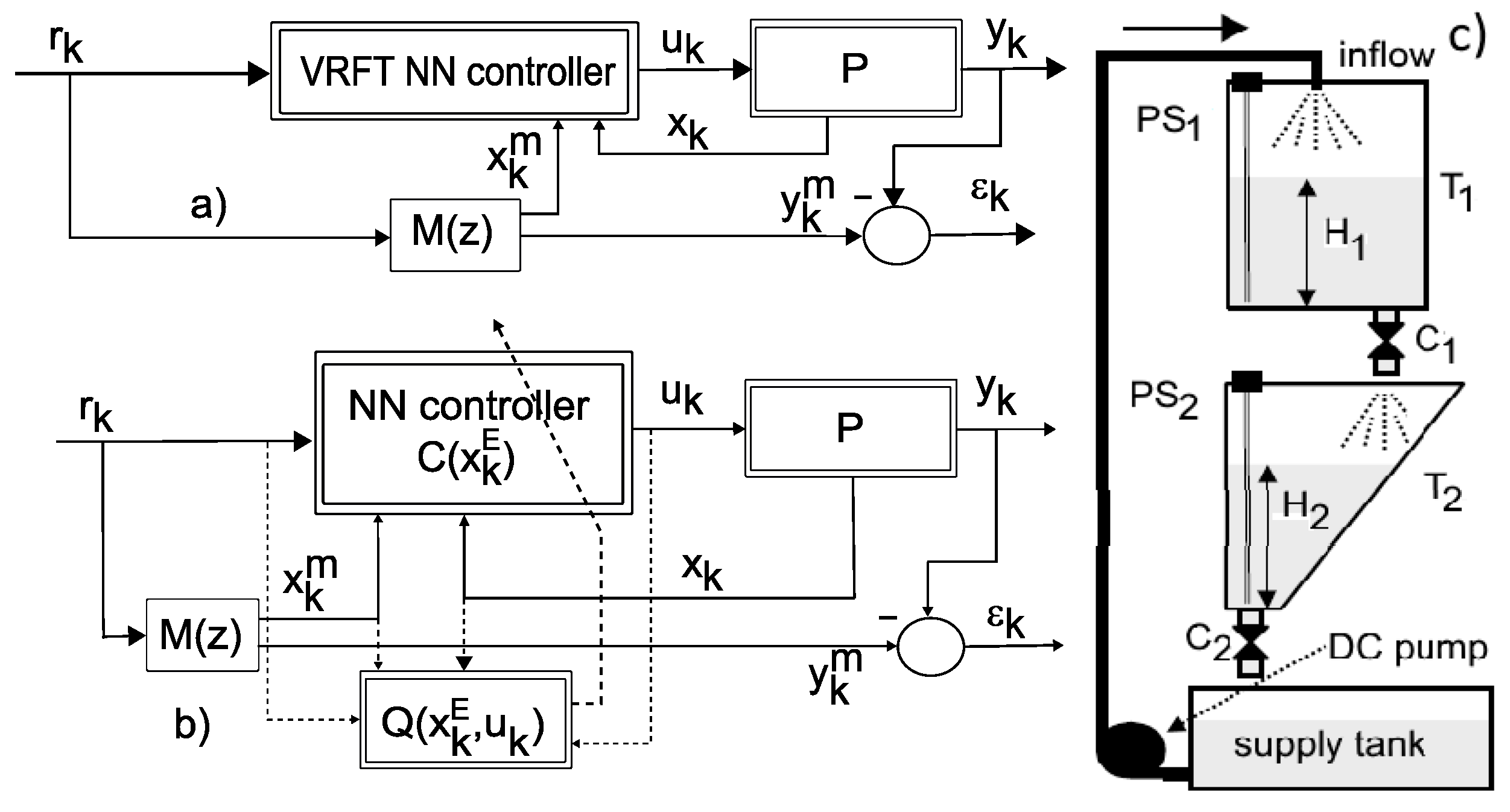
3. Nonlinear State-Feedback VRFT for Approximate ORM Tracking Control Using Neural Networks

An initial controller for the system (3) to achieve approximate ORM tracking employs the VRFT concept. Under assumptions A1 and A2, for tuning a nonlinear state-feedback controller, the designer may employ an input-state-output dataset of the form $\{{\tilde{u}}_k,{\tilde{x}}_k,{\tilde{y}}_k\},k=\overline{0,N-1}$, gathered from the process in an open-loop experiment lasting for N sample time steps, where persistently exciting ${\tilde{u}}_k$ excites all the significant process dynamics. To achieve linear ORM tracking for a nonlinear process, a nonlinear state-feedback controller is more suitable than a linear one, being able to cope with the process nonlinearities.

VRFT concept assumes that, if the controlled output y_k produced in an open-loop experiment conducted on the stable process is both the control system’s output and the ORM’s output, then the closed-loop control system will match the reference model [4,39,40,41,42]. Let ${\tilde{r}}_k=M{(z)}^{-1}{\tilde{y}}_k$ be the virtual reference input that generates ${\tilde{y}}_k$ when filtered through M(z) which is assumed to be invertible with respect to the inverse filtering operation. It is called virtual since it is never set as a reference input to the closed-loop control system and it is only used in the offline controller tuning. The virtual states of the ORM are computable from Equation (2) as ${\tilde{x}}_{k+1}^m=f^m({\tilde{x}}_k^m,{\tilde{r}}_k)$ serving to reconstruct the virtual extended state as ${\tilde{x}}_k^E={[{\left({\tilde{x}}_k\right)}^T {\left({\tilde{x}}_k^m\right)}^T {\left({\tilde{r}}_k\right)}^T]}^T$ A controller that produces ${\tilde{u}}_k$ when fed by ${\tilde{x}}_k^E$ achieves the ORM tracking. VRFT translates the model reference tracking c.f. in Equation (5) to a controller identification c.f. A finite-time controller identification c.f. is [4]

$$J_{VR}^N(\mathsf{\theta })={\displaystyle \sum _{k=0}^{N-1}{\Vert {\tilde{u}}_k^{}-C({\tilde{x}}_k^E,\mathsf{\theta })\Vert }^2}.$$

(6)

Let the optimal controller parameter vector θ^* be the solution to the optimization problem ${\mathsf{\theta }}^{*}=\arg \underset{\mathsf{\theta }}{\min }{J}_{VR}^N(\mathsf{\theta })$. Theorem 2 in [41] shows that if the controller parameterization is rich enough, then ${\mathsf{\theta }}^{*}$ also minimizes $J_{MR}^{\infty }$, proven for input-output models only. Motivated by [41], a formal proof is given as incentive for using state-feedback controllers tuned by nonlinear multi-input multi-output (MIMO) VRFT. Several other assumptions are considered:

A3: The process (1) has an equivalent input-output form $y_k=P(y_{k-1},\dots ,y_{k-ny},u_{k-1},\dots ,u_{k-nu}),$ where $ny$, $nu$ are unknown process orders and the nonlinear map $P$ is invertible with respect to $u$, meaning that for given $y_k$, $u_k$ is recoverable as $u_{k-1}=P^{-1}(y_k)$. Zero initial conditions are assumed at this point. Also, the ORM (2) has an equivalent input-output form $y_k^m=M(y_{k-1}^m,\dots ,y_{k-nym}^m,r_{k-1},\dots ,r_{k-nr})$ where $nym$, $nr$ are known ORM’s orders, M is a nonlinear invertible map with stable inverse, allowing the calculation of $r_{k-1}=M^{-1}(y_k^m)$. Zero initial conditions are also assumed.

A4: Let the process (1) and the ORM (2) be formally written as $y_k=s(x_k,u_{k-1})$ and $y_k^m=s^m(x_k^m,r_{k-1}^{})$, respectively, to capture simultaneously both the input-output dependence and the input-state-output one in a compact form. These expressions also reveal the relative degree one from input to output, without loss of generality. Assume zero initial conditions for (1) and assume the map s invertible with $x_k^{},u_{k-1}^{}$ computable from $y_k^{}$ as $x_k^{}={(s_x^{})}^{-1}(y_k^{})$, $u_{k-1}^{}={(s_u^{})}^{-1}(y_k^{})$. Further assume that $s^m$ is a continuously differentiable invertible map such that $x_k^m,r_{k-1}^{}$ are computable from $y_k^m$ as $x_k^m={(s_x^m)}^{-1}(y_k^m),r_{k-1}^{}={(s_r^m)}^{-1}(y_k^m)$ and assume there exists positive constants $B_{sx}^m>0,B_{sr}^m>0$ such that $\Vert \frac{\partial s^m(x_k^m,r_{k-1})}{\partial x_k^m}\Vert <B_{sx}^m,\Vert \frac{\partial s^m(x_k^m,r_{k-1})}{\partial r_{k-1}}\Vert <B_{sr}^m$. Let zero initial conditions hold for (2). These inversion assumptions are natural for state-space systems such as (1) and (2) that have equivalent input-output models according to A4. For example, for given output $y_k$ of (1), the input is uniquely determined as $u_{k-1}=P^{-1}(y_k)$, after which the state can be generated by recursion from $x_{k+1}=f(x_k,u_k)$ of Equation (1). This is the sense of $x_k^{}={(s_x^{})}^{-1}(y_k^{})$.

Moreover, let $s,{(s_x)}^{-1}$ be continuously differentiable and of bounded derivative to satisfy

$$\begin{array}{l}\Vert \frac{\partial s(x_k,u_{k-1})}{\partial x_k}\Vert <B_{sx},\Vert \frac{\partial s(x_k,u_{k-1})}{\partial u_{k-1}}\Vert <B_{su},\Vert \frac{\partial {(s_x)}^{-1}(y_k)}{\partial y_k}\Vert <B_{sy,}\\ 0<B_{sx}{B}_{sy}<1.\end{array}$$

(7)

A5: Let a finite open-loop trajectory collected from the process be $D=\{{\tilde{u}}_k,{\tilde{x}}_k,{\tilde{y}}_k\}\subset U\times X\times Y,k=\overline{0,N-1}$ where ${\tilde{u}}_k^{}$ is: (1) persistently exciting, for ${\tilde{y}}_k^{}$ to capture all process dynamics and (2) ensuring uniform exploration of the entire domain $U\times X\times Y$. Good exploration is achievable for large enough N.

A6: There exists a set of nonlinear parameterized state-feedback continuously differentiable controllers $\left\{C(x_k^E,\mathsf{\theta })\right\}$, a $\widehat{\mathsf{\theta }}$ for which ${\widehat{u}}_k^{}=C({\widehat{x}}_k^E,\widehat{\mathsf{\theta }})$, and an ε > 0 for which

$$J_{VR}^N(\widehat{\mathsf{\theta }})={\displaystyle \sum _{k=0}^{N-1}{\Vert {\tilde{u}}_k^{}-C({\tilde{x}}_k^E,\widehat{\mathsf{\theta }})\Vert }^2<{\mathsf{\epsilon }}^2},$$

(8)

$$\Vert \frac{\partial C(x_k^E,\mathsf{\theta })}{\partial x_k^E}\Vert <B_{cx},$$

(9)

where ${\tilde{x}}_k^E={[ {\left({\tilde{x}}_k\right)}^T {\left({\tilde{x}}_k^m\right)}^T {\left({\tilde{r}}_k\right)}^T]}^T$, ${\widehat{x}}_k^E={[ {\left({\widehat{x}}_k\right)}^T {\left({\tilde{x}}_k^m\right)}^T {\left({\tilde{r}}_k\right)}^T]}^T$ and ${\tilde{x}}_k^m={(s_x^m)}^{-1}({\tilde{y}}_k^{}),{\tilde{r}}_{k-1}^{}={(s_r^m)}^{-1}({\tilde{y}}_k^{})$. Technically, $\{{\widehat{u}}_k,{\widehat{x}}_k,{\widehat{y}}_k\}$ are generated with ${\widehat{u}}_k^{}=C({\widehat{x}}_k^E,\widehat{\mathsf{\theta }})$ in closed-loop, by processing the virtual signals ${\tilde{x}}_k^m,{\tilde{r}}_{k-1}^{}$ obtained from ${\tilde{y}}_k^{}$.

Theorem 1: Under assumptions A3–A6, there exists a finite B > 0 such that

$$J_{MR}^N(\widehat{\mathsf{\theta }})={\displaystyle \sum _{k=1}^N{\Vert {\widehat{y}}_k-{\tilde{y}}_k\Vert }_{}^2}={\displaystyle \sum _{k=1}^N{\Vert s({\widehat{x}}_k^{},{\widehat{u}}_{k-1})-s^m({\tilde{x}}_k^m,{\tilde{r}}_{k-1}^{})\Vert }_2^2}<B{\mathsf{\epsilon }}^2.$$

(10)

Proof: See Appendix A.

Corollary 1. The controller $C(x_k^E,\widehat{\mathsf{\theta }})$ obtained by minimizing the c.f. (6) is stabilizing and admissible for $J_{MR}^{\infty }$ in Equation (5) with $\mathsf{\gamma }<1$.

Proof. By Equation (8), properly identified $C(x_k^E,\widehat{\mathsf{\theta }})$ renders the finite-time $J_{MR}^N(\widehat{\mathsf{\theta }})$ (10) arbitrarily small. Secondly, a good exploration of U × X × Y ensured by $D=\{{\tilde{u}}_k,{\tilde{x}}_k,{\tilde{y}}_k\}$ reflects in good exploration of domains $R_m,X_m$ by ${\tilde{r}}_k^{},{\tilde{x}}_k^m$ respectively. In (10), ${\widehat{u}}_k,{\widehat{x}}_k,{\widehat{y}}_k,{\tilde{x}}_k^m,{\widehat{x}}_k^E,{\tilde{x}}_k^E$ are all generated from the same ${\tilde{r}}_k^{}$. If (10) holds for many combinations ${\tilde{r}}_k^{},{\tilde{x}}_k^m$ rendered form exploratory data, then by the arguments of continuous differentiability and bounded derivatives of the maps (7) and by assumption A4, they will hold for any possible combination of $r_k^{}$ and $x_k^m=f^m(x_{k-1}^m,r_{k-1})$ generated from any $r_k^{}$.

To show this, note that both ${\tilde{y}}_k=y_k^m=s^m({\tilde{x}}_k^m,{\tilde{r}}_{k-1}^{})$ and ${\widehat{y}}_k=y_k=s({\widehat{x}}_k,u_{k-1})=s({\widehat{x}}_k,C({\widehat{x}}_{k-1}^E,\widehat{\mathsf{\theta }}))$ in (10) can be generated from the same ${\tilde{r}}_k^{}$ (${\widehat{x}}_{k-1}^E$ contains ${\tilde{r}}_{k-1}^{}$). Using this fact, it follows from (10) that the ORM tracking errors $\Vert s({\widehat{x}}_k,C({\widehat{x}}_{k-1}^E({\tilde{r}}_{k-1}^{(1)})))-s_{}^m({\tilde{x}}_k^m,{\tilde{r}}_{k-1}^{(1)})\Vert$ and $\Vert s({\widehat{x}}_k,C({\widehat{x}}_{k-1}^E({\tilde{r}}_{k-1}^{(2)})))-s_{}^m({\tilde{x}}_k^m,{\tilde{r}}_{k-1}^{(2)})\Vert$ are bounded at each time step, for any two training pairs ${\tilde{r}}_{k-1}^{(1)}$ and ${\tilde{r}}_{k-1}^{(2)}$, since the sum in (10) is bounded. Then, for any $r_k^{}$ such that ${\tilde{r}}_{k-1}^{(1)}\le r_k\le {\tilde{r}}_{k-1}^{(2)}$ (component wise), since $s,s^m$ are differentiable with bounded derivatives with respect to their arguments, it must hold that $\Vert s({\widehat{x}}_k,C({\widehat{x}}_{k-1}^E(r_{k-1}^{})))-s_{}^m(x_k^m,r_{k-1}^{})\Vert =\Vert {\widehat{y}}_k-y_k^m\Vert$ is bounded. Which makes the controller $C(x_k^E,\widehat{\mathsf{\theta }})$ stabilizing for the control system in the sense of bounded output when $r_k^{}$ is bounded. Then, it is an admissible one for the infinite horizon c.f. $J_{MR}^{\infty }$ with γ < 1. This proves the claim.

An NN can be used as a controller for nonlinear state-feedback control learning. Nonlinear VRFT is proposed in [41,42] and successfully applied to NN controllers in [41,43,44,45] but only for output feedback control and not for state-feedback control as in here.

Notice that VRFT control does not need the entire extended state ${\tilde{x}}_k^E$ for feedback (i.e. including the virtual states of the ORM), the process’ initial states would suffice for this purpose. However, state extension is required for preserving the Markov property of the system (3) in order to ensure the correct collection of the transition samples; this is not possible otherwise without special collection design such as using a zero-order-hold for two-by-two consecutive time samples [43]. Correct transition samples collection is required for adaptive actor-critic tuning approach of the same NN controller that is initially tuned via VRFT.

Notice that in the proposed state-feedback VRFT design, knowledge of the output function $y_k=g(x_k)$ in Equation (1) is again not needed since ${\tilde{y}}_k$ is used to calculate the virtual reference ${\tilde{r}}_k$, while the controller only uses ${\tilde{x}}_k^E$ for feedback purposes.

4. Adaptive Actor-Critic Learning for ORM Tracking Control

If the system dynamics (3) is known, for a finite-time horizon version of the c.f. (4), numerical dynamic programming solutions can be employed backwards in time only with finite state and action spaces of moderate size, an issue referred to as the “curse of dimensionality”. For infinite horizon c.f.s, Policy Iteration and Value Iteration [23] can be used even for large and/or continuous state and action spaces, where FAs such as NNs are one option.

If the system dynamics in (3) is unknown, the minimization of the c.f. (4) becomes an RL problem. To solve it model-free, an informative c.f. for each state-action pair is defined, called the Q-function (or action-value function). With this respect, the action-value function of acting $u_k$ in state $x_k^E$ and then following the control (policy) $u_k=C(x_k^E)$ is defined as

$$Q^C(x_k^E,u_k)=V(x_k^E,u_k^{})+\mathsf{\gamma }{Q}^C(x_{k+1}^E,C(x_{k+1}^E)).$$

(11)

The optimal Q-function $Q^{*}(x_k^E,u_k^{*})$ satisfies Bellman’s optimality equation

$$Q^{*}(x_k^E,u_k^{*})=\underset{u_k^{}}{\min }\left(V(x_k^E,u_k^{})+\mathsf{\gamma }{Q}^{*}(x_{k+1}^E,u_{k+1}^{*})\right),$$

(12)

with the optimal controller and optimal Q-function

$$u_k^{*}=C^{*}(x_k^E)=\arg \underset{C}{\min }{Q}^C(x_k^E,u_k)=\arg \underset{u}{\min }{Q}^{*}(x_k^E,u).$$

(13)

Then $J^{*}(x_k^E)=Q^{*}(x_k^E,u_k^{*})$, where $J^{*}(x_k^E)=\underset{u}{\min }J(x_k^E,u)$ is the minimum value c.f. out of the c.f.s defined in Equation (4). Notice that c.f. (4) encompasses (5) thus making the ORM tracking problem consistent with the above equations. The optimal Q-function can be found using Policy Iteration or Value Iteration in a model-free manner, using, e.g., NNs as FAs. The optimal Q-function estimate and the optimal controller estimate can be updated from the transition samples in several ways: in online/offline mode, batch mode, or sample-by-sample update [23,46]. A particular class of online RL approaches is represented by the temporal difference-based AAC design that differs from the batch PI and VI approaches, as it avoids alternate batch back-up of the Q-function FA and of the controller FA.

4.1. Adaptive Actor-Critic Design

The proposed AAC design is a gradient-based scheme designed to converge to the optimal Q-function and optimal controller estimates. Let the temporal-difference error be measured from data as

$${\delta }_k(x_{k-1}^E,u_{k-1})=Ʋ(x_{k-1}^E,u_{k-1})+\mathsf{\gamma }{\widehat{Q}}_{k-1}(x_k^E,C_k(x_k^E))-{\widehat{Q}}_{k-1}(x_{k-1}^E,u_{k-1})$$

(14)

where the continuous function ${\widehat{Q}}_k(\cdot ,\cdot )$ in its arguments is the Q-function estimate at time k, time at which some controller C_k(x_k) is also available. From this point onward, for notation simplicity, x_k or plain x are used instead of x_k^E The proposed AAC design attempts the Q-function update to online minimize the c.f. E_{c, k} = 0.5 δ _k², while the controller attempts to online minimize the Q-function using gradient descent. Taxonomically, the proposed AAC belongs to the online Policy Iteration schemes where the policy evaluation step (of Bellman error residual minimization type) interleaves with the policy improvement step. The update laws for the AAC design from input-state data are:

$$u_k=C_k(x)=C_{k-1}(x)-{\mathsf{\alpha }}_a\cdot {\frac{\partial {\widehat{Q}}_{k-1}\left(x,u\right)}{\partial u}|}_{u_{k-1}},\forall x,$$

(15)

$$\begin{array}{l}{\widehat{Q}}_k\left(x_{k-1},u_{k-1}\right)={\widehat{Q}}_{k-1}\left(x_{k-1},u_{k-1}\right)+{\mathsf{\alpha }}_c{\mathsf{\delta }}_k=\\ ={\widehat{Q}}_{k-1}\left(x_{k-1},u_{k-1}\right)+{\mathsf{\alpha }}_c(Ʋ(x_{k-1},u_{k-1})+\mathsf{\gamma }{\widehat{Q}}_{k-1}(x_k,u_k=C_k(x_k))-{\widehat{Q}}_{k-1}(x_{k-1},u_{k-1})),\end{array}$$

(16)

where ${\mathsf{\alpha }}_a>0$, ${\mathsf{\alpha }}_c>0$ are learning rates. The controller $C(x_k)$ is imagined as a function (or as an infinitely dense table) mapping any state to a control action.

Comment 1: In particular, for any admissible controller $C_0$, repeated calls of (16), under proper exploration (translated to visiting all the pairs $(x_{k-1}^{},u_{k-1})\in X^E\times U$ often and to generating the sample $x_k^{}$), and under proper selection of ${\mathsf{\alpha }}_c>0$, will update ${\widehat{Q}}_k\left(x,u\right)$, $\forall x\in X^E$ until ${\mathsf{\delta }}_k^{}=0$ at which point (11) must hold and the converged $Q^{C_0}(x_k,u_k)$ evaluates $C_0$. This is an online off-policy model-free policy evaluation step. Then $Q_0\left(x,u\right)=Q^{C_0}\left(x,u\right)$ can be an initialization for AAC. Whereas, an initial admissible controller can be obtained for example using VRFT as shown later in the case study.

Comment 2: The converged Q-function of an admissible control C₀, be it Q^C₀(x_k, u_k), is positive by definition since it accumulates stage costs Ʋ > 0. Moreover, it is always greater than the optimal Q-function, i.e., Q^C₀(x_k, u_k) ≥ Q^*(x_k, u_k) > 0 and obeys the Bellman equation.

Comment 3: From (15), it follows that

$$Q_{k-1}(x,C_k(x))\le Q_{k-1}(x,C_{k-1}(x)),\forall x\in X^E$$

(17)

for a small enough ${\mathsf{\alpha }}_a>0$.

Lemma 1. Starting from an admissible controller C₀ with corresponding Q-function initialization ${\widehat{Q}}_0\left(x,u\right)=Q^{C_0}\left(x,u\right)$, the sequence $\{{\widehat{Q}}_k(x,u)\}$ is monotonic and non-increasing ensuring that

$${\widehat{Q}}_k(x,u)\le {\widehat{Q}}_{k-1}(x,u),(x,u)\in X^E\times U$$

(18)

Proof. ${\widehat{Q}}_0\left(x,u\right)$ is initialization for Equation (16) and obeys the Bellman Equation (11) for the admissible controller C₀, i.e.,

$${\widehat{Q}}_0(x_k^{},u_k)=Ʋ(x_k^{},u_k^{})+\mathsf{\gamma }{\widehat{Q}}_0(x_{k+1}^{},C_0(x_{k+1}^{})).$$

(19)

Starting the AAC update law from initial state $x_0$, $C_1(x)$ is updated first by Equation (15), then it follows that

$${\widehat{Q}}_1(x_0^{},u)={\widehat{Q}}_0(x_0^{},u)+{\mathsf{\alpha }}_c\left(\underset{\stackrel{(18)}{=}{\widehat{Q}}_0(x_0^{},C_0(x_0))}{\underbrace{Ʋ(x_0^{},u)+\mathsf{\gamma }{\widehat{Q}}_0(x_1^{},C_1(x_1))}}-{\widehat{Q}}_0(x_0^{},u)\right)={\widehat{Q}}_0(x_0^{},u)\le {\widehat{Q}}_0(x_0^{},u),\forall u.$$

(20)

Since x₀ can be any state x ∈ X^E, then Equation (18) holds for $k=1$. Assume by induction that (18) holds for some k. Using Comment 3, it follows that

$$\begin{array}{l}{\widehat{Q}}_{k+1}(x_k^{},u_k)={\widehat{Q}}_k(x_k^{},u_k)+{\mathsf{\alpha }}_c\left(Ʋ(x_k^{},u_k)+\mathsf{\gamma }{\widehat{Q}}_k(x_{k+1}^{},C_{k+1}(x_{k+1}))-{\widehat{Q}}_k(x_k^{},u_k)\right)\\ \le {\widehat{Q}}_k(x_k^{},u_k)+{\mathsf{\alpha }}_c\left(Ʋ(x_k^{},u_k)+\mathsf{\gamma }{\widehat{Q}}_k(x_{k+1}^{},C_k(x_{k+1}))-{\widehat{Q}}_k(x_k^{},u_k)\right)\le \\ \stackrel{(18)}{\le }{\widehat{Q}}_{k-1}(x_k^{},u_k)+{\mathsf{\alpha }}_c\left(Ʋ(x_k^{},u_k)+\mathsf{\gamma }{\widehat{Q}}_{k-1}(x_{k+1}^{},C_k(x_{k+1}))-{\widehat{Q}}_{k-1}(x_k^{},u_k)\right)={\widehat{Q}}_k(x_k^{},u_k),\end{array}$$

(21)

and since $x_k,u_k$ can be any pair (x, u) ∈ X^E × U, the conclusion of Lemma 1 follows.

Theorem 2. Let ${\widehat{Q}}_0\left(x,u\right)>0$, finite for any finite argument) be an initialization for the Q-function of an initial admissible controller C₀. Starting with any x₀ the control u₀ = C₀(x₀) is applied to the process. Specifically, the AAC update laws ((15), (16)) ensures that at time k = 1, C₁ is updated from C₀, ${\widehat{Q}}_0\left(x,u\right)$ is updated with (16) using u₁ = C₁(x₁) in the right-hand side, the control u₁ is sent to the process, and then k ← 2, with the above strategy repeated for subsequent times. Claim: The feedback control system under time-varying control C_k is stabilized for γ < 1 and asymptotically stabilized for γ = 1.

Proof. It is valid for the first three time steps that

$${\widehat{Q}}_1(x_0^{},u_0)\stackrel{(16)}{=}{\widehat{Q}}_0(x_0^{},u_0)+{\mathsf{\alpha }}_c[Ʋ(x_0^{},u_0^{})+\mathsf{\gamma }{\widehat{Q}}_0(x_1^{},u_1=C_1(x_1^{}))-{\widehat{Q}}_0(x_0^{},u_0)]\stackrel{(18)}{\le }{\widehat{Q}}_0(x_0,u_0).$$

(22a)

$${\widehat{Q}}_2(x_1^{},u_1)\stackrel{(16)}{=}{\widehat{Q}}_1(x_1^{},u_1)+{\mathsf{\alpha }}_c[Ʋ(x_1^{},u_1^{})+\mathsf{\gamma }{\widehat{Q}}_1(x_2^{},u_2=C_2(x_2^{}))-{\widehat{Q}}_1(x_1^{},u_1)]\stackrel{(18)}{\le }{\widehat{Q}}_1(x_1,u_1).$$

(22b)

$${\widehat{Q}}_3(x_2^{},u_2)\stackrel{(16)}{=}{\widehat{Q}}_2(x_2^{},u_2)+{\mathsf{\alpha }}_c[Ʋ(x_2^{},u_2^{})+\mathsf{\gamma }{\widehat{Q}}_2(x_3^{},u_3=C_3(x_3^{}))-{\widehat{Q}}_2(x_2^{},u_2)]\stackrel{(18)}{\le }{\widehat{Q}}_2(x_2,u_2).$$

(22c)

Cancelling the same terms in both sides of Equation (22a–c), since ${\mathsf{\alpha }}_c>0$, it follows that the sums in square parentheses are negative. These sums are further refined using Lemma 1 as

$$Ʋ(x_0^{},u_0^{})+\mathsf{\gamma }{\widehat{Q}}_0(x_1^{},u_1)\le {\widehat{Q}}_0(x_0,u_0),$$

(23a)

$$Ʋ(x_1^{},u_1^{})+\mathsf{\gamma }{\widehat{Q}}_1(x_2^{},u_2)\le {\widehat{Q}}_1(x_1,u_1)\stackrel{(18)}{\le }{\widehat{Q}}_0(x_1,u_1),$$

(23b)

$$Ʋ(x_2^{},u_2^{})+\mathsf{\gamma }{\widehat{Q}}_2(x_3^{},u_3)\le {\widehat{Q}}_2(x_2,u_2)\stackrel{(18)}{\le }{\widehat{Q}}_1(x_2,u_2),$$

(23c)

Using (23c) in (23b) it follows that $Ʋ(x_1^{},u_1^{})+\mathsf{\gamma }Ʋ(x_1^{},u_1^{})+{\mathsf{\gamma }}^2{\widehat{Q}}_2(x_3^{},u_3)\le {\widehat{Q}}_0(x_1,u_1)$, which used in (23a) results in$Ʋ(x_0^{},u_0^{})+\mathsf{\gamma }Ʋ(x_1^{},u_1^{})+{\mathsf{\gamma }}^2Ʋ(x_2^{},u_2^{})+{\mathsf{\gamma }}^3{\widehat{Q}}_2(x_3^{},u_3)\le {\widehat{Q}}_0(x_0,u_0)$. Extending the exemplified reasoning backwards from infinity it follows that

$$\underset{N\to \infty }{\lim }\left({\displaystyle \sum _{i=0}^{N-1}{\mathsf{\gamma }}^iƲ(x_i^{},u_i^{})}+{\mathsf{\gamma }}^N{\widehat{Q}}_{N-1}(x_N,u_N)\right)\le {\widehat{Q}}_0(x_0,u_0).$$

(24)

Since $\underset{N\to \infty }{\lim }{\mathsf{\gamma }}^N{\widehat{Q}}_{N-1}(x_N,u_N)=0$ because ${\widehat{Q}}_{N-1}(x_N,u_N)$ is bounded since resulting from a non-increasing sequence, it follows that $\underset{N\to \infty }{\lim }{\displaystyle \sum _{i=0}^{N-1}{\mathsf{\gamma }}^iƲ(x_i^{},u_i^{})}\le {\widehat{Q}}_0(x_0,u_0)$ is finite. The left term in the inequality is the cost of using the controller $u_0=C_0(x_0),u_1=C_1(x_1),\dots$. Then it follows that the control system remains stable under the time-varying control of the AAC updates. Moreover, for $\mathsf{\gamma }=1$, the sequence $\left\{\sqrt{Ʋ(x_i^{},u_i^{})}\right\},i=\overline{0,\infty }$ must be square-summable which implies that the control system is asymptotically stabilized by $C_k$, thus proving the claim of the theorem.

Comment 4: The above proof resembles the stabilizing action-dependent value iteration of [30], but here relies on gradient-based updates of the Q-function estimate and of the controller, rather than on its minimization. The stability result of the Theorem 2 is valid under continuous updates of the AAC laws (15), (16) under no exploration. It ensures that, starting from an admissible controller $C_0$, the AAC updates (15), (16) preserve the control system stability. Since exploratory controls $u_k$ are critical, a compromising solution is to perform the controller update (15) only for non- exploratory sampling instants, while the Q-function estimates are continuously updated per (16).

4.2. AAC Using Neural Networks As Approximators

In practice, specific FAs such as NNs are employed as approximators for the Q-function and for the controller, respectively. Using NNs as FAs (implying nonlinear features parameterization), the convergence of the learning scheme depends on a large extent to the selection of the learning parameters. However, the advantage of using generic NN architectures is that no manual or automatic feature selection is needed for parameterizing the Q-function and controller estimates.

The proposed AAC design herein uses two NNs to approximate the Q-function (critic, referred to herein as Q-NN), and the controller (actor, referred to herein as C-NN), respectively. Assume an initial admissible NN VRFT state-feedback controller exists. Let the critic NN FA and controller NN FA be parameterized as ${\widehat{Q}}_k(x_k^E,u_k,{\mathsf{\theta }}_k^c)$ and ${\mathbf{C}}_k(x_k^E,{\mathsf{\theta }}_k^a)$, respectively. With three-layer feed-forward NNs having one hidden layer, fully connected with bias, the critic and the controller are modeled by:

$${\widehat{Q}}_k=W_{c,n_{hc}+1}^k+{\displaystyle \sum _{i=1}^{n_{hc}}{W}_{c,i}^k{\mathsf{\sigma }}_i({\displaystyle \sum _{j=1}^{n_{ic}+1}{V}_{c,ji}^k{I}_j^k})},$$

(25)

$$u_k^l=W_{a,n_{ha}+1}^{k,l}+{\displaystyle \sum _{i=1}^{n_{ha}}{W}_{a,i}^{k,l}{\mathsf{\sigma }}_i({\displaystyle \sum _{j=1}^{n_{ia}+1}{V}_{a,ji}^k{I}_j^k}),} l=\overline{1,m},$$

(26)

with $W_c={[W_{{}_{c,1}}^k \dots W_{c,n_{hc}+1}^k]}^T$—the critic output layer weights having n_hc hidden neurons, $V_c={[V_{c,ji}^k]}_{i=1\dots n_{hc},j=1\dots n_{ic}+1}$—the critic hidden layer weights matrix, $I_c^k={[I_1^k\dots I_{n_{ic}+1}^k]}^T={[{\left(x_k^E\right)}^T {\left(u_k\right)}^T 1]}^T$—the critic input vector of size n_ic + 1 (the bias input is constant 1), $W_a^{k,l}={[W_{a,1}^{k,l} \dots W_{a,n_{ha}+1}^{k,l}]}^T,l=1..m$ – the output layer weights of the l-th controller output $u_k={[u_k^1\dots u_k^m]}^T$, having n_ha hidden neurons, and $V_a={[V_{a,ji}^k]}_{i=1\dots n_{ha},j=1\dots n_{ia}+1}$—the controller hidden layer weights matrix, $I_a^k={[I_1^k\dots I_{n_{ia}+1}^k]}^T={[{\left(x_k^E\right)}^T 1]}^T$ – the controller input vector of size n_ia + 1 (bias input 1 included). σ_i = tanh_i, is the hyperbolic tangent activation function at the output of i^th hidden neuron. The controller and critic are cascaded, with the actor output u_k as a part of the critic input alongside $x_k^E$ The actor and critic weights are formally parameterized as ${\mathsf{\theta }}_a^k={[{(W_a^{k,l})}^T {(V_a^k)}^T]}^T$ and ${\mathsf{\theta }}_c^k={[{(W_c^k)}^T {(V_c^k)}^T]}^T$, respectively.

The AAC’s gradient descent tuning rules for the critic (25) and controller (26) as parameterized variants of (15) and (16) are

$$\{\begin{array}{l}{\mathsf{\theta }}_k^c={\mathsf{\theta }}_{k-1}^c+{\mathsf{\alpha }}_c\cdot {\frac{\partial \widehat{Q}\left(x,u,\mathsf{\theta }\right)}{\partial \mathsf{\theta }}|}_{(x_{k-1}^E,u_{k-1},{\mathsf{\theta }}_c^{k-1})}\cdot {\mathsf{\delta }}_k, \text{detailed as}:\\ W_{c,i}^k=W_{c,i}^{k-1}+{\mathsf{\delta }}_k{\mathsf{\alpha }}_c\times \{\begin{array}{ll}{\mathsf{\sigma }}_i({\displaystyle \sum _{j=1}^{n_{ic}+1}{V}_{c,ji}^{k-1}{I}_j^{k-1}}),& if i\ne n_{hc}^{}+1,\\ 1,& \mathrm{if} i=n_{hc}^{}+1,\end{array}\\ V_{c,ji}^k=V_{c,ji}^{k-1}+{\mathsf{\delta }}_k{\mathsf{\alpha }}_c{W}_{c,i}^{k-1}{I}_j^{k-1}{\mathsf{\sigma }}_i^{\prime }({\displaystyle \sum _{j=1}^{n_{ic}+1}{V}_{c,ji}^{k-1}{I}_j^{k-1}}),\end{array}$$

(27)

$$\{\begin{array}{l}{\mathsf{\theta }}_k^a={\mathsf{\theta }}_{k-1}^a-{\mathsf{\alpha }}_a\cdot {\frac{\partial \widehat{Q}\left(x,u,\mathsf{\theta }\right)}{\partial u}|}_{(x_{k-1}^E,u_{k-1},{\mathsf{\theta }}_c^{k-1})}\cdot {\frac{\partial u\left(x,\mathsf{\theta }\right)}{\partial \mathsf{\theta }}|}_{(x_{k-1}^E,{\mathsf{\theta }}_a^{k-1})},\mathrm{as}:\\ W_{a,i}^{k,l}=W_{a,i}^{k-1,l}-{\mathsf{\alpha }}_a\underset{{\frac{\partial \widehat{Q}\left(x,u,\mathsf{\theta }\right)}{\partial u}|}_{(x_{k-1}^E,u_{k-1},{\mathsf{\theta }}_c^{k-1})}}{\underbrace{\left({\displaystyle \sum _{i=1}^{n_{hc}}{W}_{c,i}^{k-1}{V}_{c,\xi i}^{k-1}{\mathsf{\sigma }}_i^{\prime }({\displaystyle \sum _{j=1}^{n_{ic}+1}{V}_{c,ji}^{k-1}{I}_j^{k-1}})}\right)}}\times \{\begin{array}{ll}{\mathsf{\sigma }}_i({\displaystyle \sum _{j=1}^{n_{ia}+1}{V}_{a,ji}^{k-1}{I}_j^{k-1}}),& \mathrm{if} i\ne n_{ha}+1,\\ 1,& \mathrm{if} i\ne n_{ha}+1,\end{array}\\ V_{a,ji}^k=V_{a,ji}^k-{\mathsf{\alpha }}_a{\frac{\partial \widehat{Q}\left(x,u,\mathsf{\theta }\right)}{\partial u}|}_{(x_{k-1}^E,u_{k-1},{\mathsf{\theta }}_c^{k-1})}{W}_{a,i}^{k-1,l}{I}_j^{k-1}{{\mathsf{\sigma }}^{\prime }}_i({\displaystyle \sum _{j=1}^{n_{ia}+1}{V}_{a,ji}^{k-1}{I}_j^{k-1}}),\end{array}$$

(28)

with α_a, α_c—the learning rate magnitudes of the critic and controller training rules, respectively and ${\mathsf{\sigma }}_i^{\prime }$ is the derivative of σ_i w.r.t its argument and ξ is the index of $u_k^l$ in the $I_c^k$.

In many practical applications, the designer chooses to perform either full or partial adaptation of the NNs’ weights, the latter implying only output weights adaptation. In this latter case, the Q-NN and C-NN parameterizations are:

$$\begin{array}{l}{\widehat{Q}}_k(x_k^E,u_k)={\left(W_c^k\right)}^T\mathsf{\sigma }(V_c^k{[{\left(x_k^E\right)}^T {\left(u_k\right)}^T 1]}^T)={\left(W_c^k\right)}^T{\Phi }_c^k(x_k^E,u_k), \\ u_k=C_k(x_k^E)={\left(W_a^k\right)}^T\mathsf{\sigma }(V_a^k{[{\left(x_k^E\right)}^T 1]}^T)={\left(W_a^k\right)}^T{\Phi }_c^k(x_k^E),\end{array}$$

(29)

where ${\Phi }_c^k(x_k^E,u_k),{\Phi }_a^k(x_k^E)$ are the matrices of basis functions (or input features) and W_c^k, W_a^k are the tunable output weights parameters, rendering ${\widehat{Q}}_k,u_k$ as linear combination of basis functions. This linear parameterization simplifies the convergence analysis but also requires manual features selection and training as a disadvantage.

As it is well-known, the AAC architecture performs online with the C-NN sending controls to the process and the Q-NN serving both to estimate the Q-function and to adaptively tune the C-NN. The closed-loop control system with the process (3) combined with the AAC tuning rules (27), (28) has the unique property that its dynamics is mainly driven by the reference input r_k viewed as a particular state of the extended state vector and, possibly, by exogenous unknown disturbances. Since r_k is user selectable, it can be used to drive the control system in a wide operating range to ensure efficient exploration of the state space. Enhanced exploration of the domain X^E × U can be performed by trying random actions in every state, usually as additive uniform random actions.

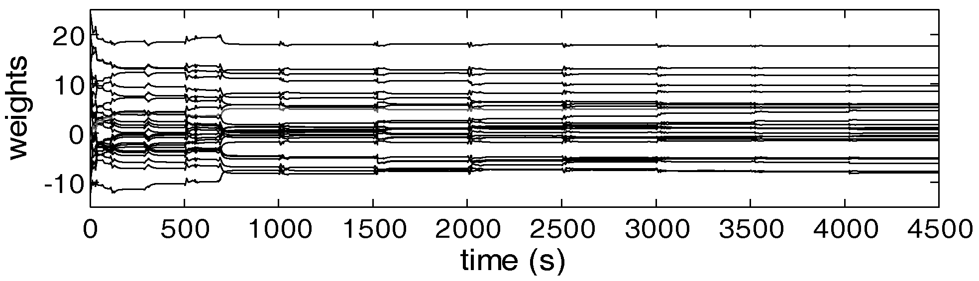
4.3. Convergence of the AAC Learning Scheme with NNs

While the results from Section 4.1 are formulated under generic functions for the Q-function and for the controller, the convergence to the optimal controller and optimal Q-function is not ensured. In the following, the convergence to of the AAC learning with NNs is shown. Linear parameterization is the most widely used and supports tractable analysis. Let the output weight parameterization (29) of the Q-NN and C-NN lead to the update laws

$$\begin{array}{l}{W}_c^k=W_c^{k-1}+{\mathsf{\alpha }}_c{\mathsf{\delta }}_k{\Phi }_c^k(x_{k-1}^E,u_{k-1}), \\ W_a^k=W_a^{k-1}-{\mathsf{\alpha }}_a{\Phi }_a^k(x_{k-1}^E){\left(W_c^{k-1}\right)}^T\frac{\partial {\Phi }_c}{\partial u}(x_{k-1}^E,u_{k-1}),\end{array}$$

(30)

be compactly written as

$$\begin{array}{l}{W}_c^k=W_c^{k-1}+{\mathsf{\alpha }}_c{\mathsf{\delta }}_k{\Phi }_c^{k-1}, \\ W_a^k=W_a^{k-1}-{\mathsf{\alpha }}_a{\Phi }_a^{k-1}{\left(W_c^{k-1}\right)}^T{\Phi }_{c,u}^{k-1},\end{array}$$

(31)

where ${\mathsf{\delta }}_k=\underset{U^{k-1}}{\underbrace{Ʋ(x_{k-1}^E,u_{k-1})}}+{\left(W_c^{k-1}\right)}^T\left(\mathsf{\gamma }{\Phi }_c^k-{\Phi }_c^{k-1}\right)$ Let the weights of the optimal Q-NN and optimal C-NN be W_c^*, W_a^*, the estimation errors being ${\tilde{W}}_c^k=W_c^k-W_c^{*},{\tilde{W}}_a^k=W_a^k-W_a^{*}$ that render the estimation error dynamics

$$\begin{array}{l}{\tilde{W}}_c^k={\tilde{W}}_c^{k-1}+{\mathsf{\alpha }}_c{\mathsf{\delta }}_k{\Phi }_c^{k-1}, \\ {\tilde{W}}_a^k={\tilde{W}}_a^{k-1}-{\mathsf{\alpha }}_a{\Phi }_a^{k-1}{\left(W_c^{k-1}\right)}^T{\Phi }_{c,u}^{k-1},\end{array}$$

(32)

Some assumptions follow:

A7. Let the estimation error of the critic be denoted as ${\mathsf{\zeta }}_c^{k-1}={\left({\tilde{W}}_c^{k-1}\right)}^T{\Phi }_c^{k-1}$, let the critic’s and actor’s hidden activation layers be bounded as ${\Vert {\Phi }_c^{k-1}\Vert }^2\le {\overline{\mathsf{\phi }}}_c,{\Vert {\Phi }_a^{k-1}\Vert }^2\le {\overline{\mathsf{\phi }}}_a$ and let the critic’s activation layer derivative w.r.t. u be bounded as ${\Vert {\Phi }_{c,u}^{k-1}\Vert }^2\le {\overline{\mathsf{\phi }}}_{c,u}$ where Frobenius norm was used, which is equivalent to the Euclidean norm when it is applied to vectors. The above upper bounds follow since the activation functions are bounded and so are their derivatives.

Theorem 3. Under A7, the AAC learning scheme converges to a vicinity of the optimal controller and optimal Q-function since the estimation errors ${\tilde{W}}_c^k,{\tilde{W}}_a^k$ are uniformly ultimately bounded provided that ${\mathsf{\alpha }}_c>4{\overline{\mathsf{\phi }}}_c^2-2{\overline{\mathsf{\phi }}}_c+1$, for ${\overline{\mathsf{\phi }}}_c>1$.

Proof: See Appendix B.

Comment 5. Notice that the temporal difference error ${\mathsf{\delta }}_k$ is calculated in terms of the Q-NN’s output. Then ${\mathsf{\delta }}_k$ is backpropagated to correct the Q-NN weights. Moreover, ${\mathsf{\delta }}_k$ is further backpropagated to correct the C-NN weights, since the C-NN output is an input to the Q-NN. Hence, the resulted AAC architecture belongs to the deep learning approaches (the architecture is presented in Figure 1b of the next Section).

4.4. Summary of the Mixed VRFT-AAC Design Approach

The steps of the VRFT-AAC design approach are summarized next:

S1. Collect input-state-output samples from the open-loop stable process (1) in a dataset $D=\{{\tilde{u}}_k,{\tilde{x}}_k,{\tilde{y}}_k\}\subset U\times X\times Y,k=\overline{0,N-1}$ where ${\tilde{u}}_k^{}$ persistently exciting, under conditions of A5.

S2. Obtain the initial state-feedback VRFT controller by minimizing the c.f. in Equation (6) as ${\mathsf{\theta }}_k^a=\arg \underset{\mathsf{\theta }}{\min }{J}_{VR}^N(\mathsf{\theta })$. When NNs are used, minimization of the c.f. (6) is equivalent to training the NN. The obtained controller is $C_k(x_k^E,{\mathsf{\theta }}_k^a)$, which is a controller for both the process (1) and for the extended process (3). It is also a close initialization to the optimal controller that minimizes $J_{MR}^{\infty }$ from (5), since VRFT identifies a controller that approximately minimizes $J_{MR}^N$ from (10) as a finite horizon version of $J_{MR}^{\infty }$. This is supported by Theorem 1.

S3. Close the control system loop on process (1) (it is equivalent to closing it on extended process (3)) using controller $C_k(x_k^E,{\mathsf{\theta }}_k^a)$. The architecture is presented in Figure 2b). Use update (16) (in explicitly parameterized form, use (28)) under an exploratory reference input $r_k$ in order to learn the Q-function of the controller $C_k(x_k^E,{\mathsf{\theta }}_k^a)$. This serves as properly initializing ${\widehat{Q}}_k(x_k^E,u_k,{\mathsf{\theta }}_k^c)$ for the subsequent AAC tuning.

S4. Use the updates (15), (16), (27), (28), in explicitly parameterized form), in this exact order and under an exploratory reference input $r_k$, to learn the optimal controller $C^{*}(x_k^E,{\mathsf{\theta }}_k^a{}^{*}=W_a^{*})$ and the optimal Q-function ${\widehat{Q}}^{*}(x_k^E,u_k,{\mathsf{\theta }}_k^c{}^{*}=W_c^{*})$. Using the above updates for a finite time on a random learning scenario is called a learning episode.

S5. After every learning episode, measure the tracking performance on a standard test scenario. When the prescribed number of maximum tests is reached or the tracking performance on the standard scenario is not improving anymore, the controller learning is stopped. Otherwise, proceed to the next learning episode.

All implementation details of the above VRFT-AAC design are presented in the following Section 5.1 when validation is performed on the complex multivariable tank system case study.

5. Validation Case Study

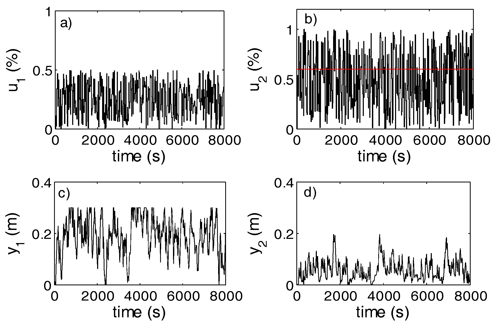
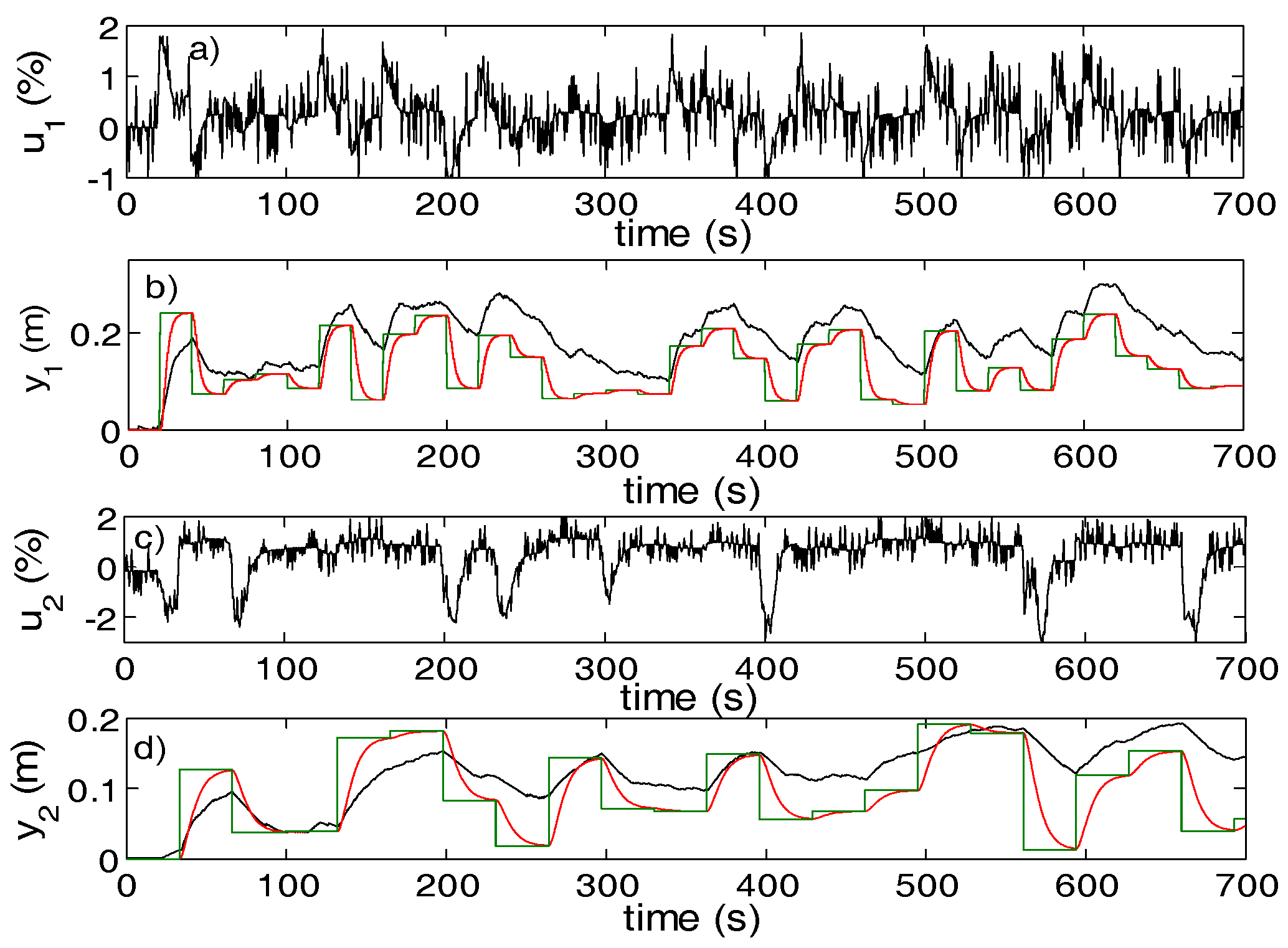
5.1. AAC Design for a MIMO Vertical Tank System

The controlled process is a vertical MIMO two-tank system (Figure 1c) built around a three-tank laboratory equipment [47] with the continuous-time state-space equations

$$\begin{array}{l}{\dot{H}}_1=\frac{k}{aw}{u}_1-\frac{1}{aw}{\overline{C}}_1{H}_1^{\mathsf{\alpha }1}(2.5{\tilde{u}}_2-0.5),\\ {\dot{H}}_2=\frac{1}{aw}{\overline{C}}_1{H}_1^{\mathsf{\alpha }1}(2.5{\tilde{u}}_2-0.5)-\frac{1}{cw+\frac{H_2}{H_{2\max }}bw}{\overline{C}}_2{H}_2^{\mathsf{\alpha }2},\\ \hspace{0.17em}\hspace{0.17em}\hspace{0.17em}\hspace{0.17em}\hspace{0.17em}\hspace{0.17em}\hspace{0.17em}\hspace{0.17em}\hspace{0.17em}\hspace{0.17em}\hspace{0.17em}{\tilde{u}}_2=\min (\max (u_2,0.6),1),\end{array}$$

(33)

with $a=0.25 [\mathrm{m}]$, $w=0.035 [\mathrm{m}]$, $c=0.1 [\mathrm{m}]$, $b=0.345 [\mathrm{m}]$ and $H_{1\max }=H_{2\max }=0.35 [\mathrm{m}]$. $x_1=y_1=H_1\in [0,H_{1\max }]$ and $x_2=y_2=H_2\in [0,H_{2\max }]$ are the water levels in the two tanks considered as system states and controlled outputs. The control inputs $u_1,u_2\in [0,1]$ (also expressible in [%]) are the duty cycles of the pump direct current (DC) motor and of the electrically controlled valve $C_1$, respectively. $k=1.66\cdot {10}^{-4}[m^3/(s\cdot \%)]$ is the gain from the pump input to the inflow, ${\overline{C}}_1=5.65\cdot {10}^{-5}[m^{3-\mathsf{\alpha }1}/s]$, ${\overline{C}}_2=8\cdot {10}^{-5}[m^{3-\mathsf{\alpha }2}/s]$ are the resistances of the outflow orifices of the first (upper) and second (lower) tank, called $T_1$ and $T_2$, respectively, and α₁ = 0.29, α₂ = 0.22. The third equality in Equation (33) reflects the dead-zone plus saturation in the second control input u₂.

Features of this process include: no water level setpoint for the tank $T_2$ can be set if the water level in $T_1$ is zero; the electrical valve controlling the outflow from $T_1$ (which is inflow to $T_2$) is changed by ${\tilde{u}}_2(u_2)$; no setpoint can be tracked for each tank if there is more outflow than inflow; $T_1$’s outflow has a minimum value and can be zero only when $H_1=0$, as per first equality in (33). $T_2$’s dynamics is slower than $T_1$’s. Proper selection of the parameters ${\overline{C}}_1,{\overline{C}}_2$ through manual valves allows feasible control trajectories in the constrained input-state-output space. Discretization of (33) reveals its Markov form. The water level is measured using piezoelectric sensors ($P{S}_1$ and $P{S}_2$ in Figure 1c). Protection logic disables the pump voltage when water level exceeds the upper bound. The sampling period used for control experiments is $T_s=0.5 \mathrm{s}$. Model (33) is not used for control design.

For VRFT-based control design, the ORM is selected as the ZOH discretization of $M(s)=diag(M_1(s),M_2(s))$. $M_1(s)={\mathsf{\omega }}_0^2/(s^2+2\mathsf{\varsigma }{\mathsf{\omega }}_{0}s+{\mathsf{\omega }}_0^2)$, with the damping factor $\mathsf{\varsigma }=1.0$ and the natural frequency ${\mathsf{\omega }}_0=0.5rad/s$ selects the speed and shape of the desired response $y_{k,1}^m$ while similar $M_2(s)$ with $\mathsf{\varsigma }=1.0$ and ${\mathsf{\omega }}_0=0.2rad/s$ describes $y_{k,2}^m$. For collecting the open-loop input-state-output data ${\{{\tilde{u}}_k,{\tilde{x}}_k,{\tilde{y}}_k\}}_{k=0\dots N-1}$, 16,000 samples have been generated from 16,000 samples of a uniformly random sequence of persistently exciting steps lasting for 20 s ${\tilde{u}}_k={[{\tilde{u}}_{k,1} {\tilde{u}}_{k,2}]}^T\in [0,0.5]\times [0,1]$, for an experiment of 8000 s. The collected data is displayed in Figure 2 and ensures the exploratory conditions from Assumption A5.

The controllable canonical state-space realizations (A₁, B₁, C₁, D₁) and $(A_2,B_2,C_2,D_2)$ and of $M_1(z)$ and $M_2(z)$ are, respectively:

$$\begin{array}{l}{A}_1=\left(\begin{array}{cc}1.5576& -0.6065\\ 1& 0\end{array}\right),B_1=\left(\begin{array}{c}1\\ 0\end{array}\right),C_1^{}={\left(\begin{array}{l}0.0265\\ 0.0224\end{array}\right)}^T,D_1=0,\\ A_2=\left(\begin{array}{cc}1.8097& -0.8187\\ 1& 0\end{array}\right),B_2=\left(\begin{array}{c}1\\ 0\end{array}\right),C_2^{}={\left(\begin{array}{l}0.0047\\ 0.0044\end{array}\right)}^T,D_2=0,\end{array}$$

(34)

The ORM state will then be $x_k^m={[x_{k,1}^m x_{k,2}^m x_{k,3}^m x_{k,4}^m]}^T$. The virtual reference ${\overline{r}}_k=M{(z)}^{-1}{\tilde{y}}_k$ is used as input to the state-space models (34) to obtain the ORM’s virtual states ${\tilde{x}}_k^m$. The extended virtual state vector ${\tilde{x}}_k^E={[ {\left({\tilde{x}}_k\right)}^T {\left({\tilde{x}}_k^m\right)}^T {\left({\tilde{r}}_k\right)}^T]}^T\in {\Re }^8$ is used to offline compute the C-NN via VRFT by fitting the inputs ${\tilde{x}}_k^E$ to the outputs ${\tilde{u}}_k$. Note that using two second order ORM’s produces four states in the extended state-space, which is disadvantageous. The ORM’s orders should to be as low as possible (usually one) but a second order model offers greater flexibility in output response shaping.

The VRFT C-NN architecture (Figure 1a) is a feedforward 8–10–2 fully connected one with biases having $n_{ha}=10$ hidden neurons with $\tanh ( )$ activation function and the output activation functions are linear. The weights are initialized with random uniform numbers in $[-1.5,1.5]$. Since the NN training is performed offline, standard gradient backpropagation training with Levernberg-Marquardt [48] is used for maximum 50 epochs to learn a stabilizing VRFT C-NN controller $C(x_k^E)$ for the MIMO control system, that minimizes $J_{VR}^N$. 80% of the data is effectively used for training while the rest of 20% serves as validation data. Early stopping is used after six consecutive increases in the mean sum of squared error evaluated on the validation data. Other offline training algorithms such as Broyden-Fletcher-Goldfarb-Shanno [49,50] and conjugate gradient [51,52] may be similarly efficient while their computational burden is prohibitive for online real-time training.

Results on a standard test scenario with the initial VRFT C-NN controller are shown in Figure 3. It is observed that the ORM tracking errors are bounded, since the VRFT controller is stabilizing (though not asymptotically) and validates the theoretical results of Theorem 1 and Corollary 1. Then it is an admissible controller for $J_{MR}^{\infty }$ in Equation (5) with $\mathsf{\gamma }<1$. The initial controller tuning using VRFT is attractive also because it has learned a feature matrix ${\Phi }_a(x_k^E)$, so from this point onwards, the designer can choose to perform either output weights adaptation or full weights adaptation.

The Q-function estimate of the VRFT C-NN (i.e., the critic Q-NN) is next learned in a policy evaluation step in order to serve as a good initial estimate of the Q-function that is needed for the following AAC learning and also to fulfil the requirements of Lemma 1. This step is possible since the VRFT controller is admissible and, for properly selected learning rate, the weights of the Q-NN will converge. The critic Q-NN approximating the Q-function has similar architecture with the C-NN, of size 10–25–1 (eight states and two controls), with $n_{hc}=25$. The critic Q-NN output weights are randomly drawn from a zero-mean normal distribution with variance ${\mathsf{\sigma }}^2=90$ while the hidden layer weighs are uniformly randomly initialized in $[-1.5,1.5]$. Setting $\mathsf{\gamma }=0.95$, the learning rates ${\mathsf{\alpha }}_c=0.01$ in (27) and ${\mathsf{\alpha }}_a=0$ in (28) (no controller tuning), all the Q-NN weights are updated using the gradient back-propagation in (27), by driving the MIMO control system with a sequence of uniformly random piecewise constant steps in $r_k={[r_{k,1} r_{k,2}]}^T\in [0.05,0.25]\times [0.01,0.2]$. This procedure also serves as a tuning step for ${\mathsf{\alpha }}_c$. With $r_{k,1}$ and $r_{k,2}$ lasting 20 s and 33 s, respectively, we ensure they do not switch simultaneously, to better reveal the coupling effects between the control channels. After 500 s, the critic weights stabilize, the output weights being shown in Figure 4 for 4500 s. This pre-tuned Q-NN will be used as initialization to the following case studies. After this intermediate tuning step of the Q-NN, the designer can choose for full weight adaptation of the Q-NN or only for output weights’ adaptation of the Q-NN while the features matrix ${\Phi }_c(x_k^E,u_k)$ is kept constant.

The C-NN is now further tuned (in the architecture from Figure 1b to improve the ORM control performance. Setting ${\mathsf{\alpha }}_a={10}^{-8}$ in (28) and ${\mathsf{\alpha }}_c=0.01$ in (27) (critic adaptation should generally be faster than actor adaptation), both the C-NN and Q-NN are adaptively trained online. Although carried out in an adaptive framework, the training unfolds on consecutive episodes where the feedback control system is driven by a sequence of random reference input steps for 700 s. The reference inputs are uniformly random piecewise constant steps in $r_k={[r_{k,1} r_{k,2}]}^T\in [0.05,0.25]\times [0.01,0.2]$, with $r_{k,1}$ and $r_{k,2}$ lasting 20 s and 33 s, respectively. Updates (27), (28) are skipped when either $r_{k,1}$ or $r_{k,2}$ switch, to preserve the Markov property of the extended model. The controller parameters at the end of an episode are the initial ones for the following episode, the Q-NN weights following the same transfer rule. To ensure enhanced exploration of the state-action space, the C-NN controller output is perturbed every third sample time with probing noise according to:

$$u_k=C(x_k^E)+\left(\begin{array}{l}rand\\ rand\end{array}\right)\cdot \mathrm{\Omega },\mathrm{\Omega }=\{\begin{array}{cc}1& \mathrm{if} \mathrm{mod}(k,3) = 0,\\ 0& \mathrm{otherwise},\end{array}$$

(35)

where $rand$ is a normally distributed random number with zero-mean and variance ${\mathsf{\sigma }}^2=3.56$ and $\mathrm{mod}(k,s)$ is the remainder after dividing k by s. This is in fact a form of ε⁰-greedy exploration strategy useful to try many actions in the vicinity of the current state. A typical learning episode is shown in Figure 5. After each learning episode, the learning is stopped and the C-NN performance is measured on the standard test scenario from Figure 3 and the decrease of a finite-time version of the c.f. $J_{MR}^{\infty }$ from Equation (5), namely $J_{MR}^{1400}$, is aimed. This standard test scenario is not seen during training. The learning then resumes with the next episode. After maximum 30 learning episodes (meaning 21,000 s and 42,000 samples), the C-NN and Q-NN adaptations are stopped and the learning trial (comprising of learning episodes) converges under Theorem 3. The final adaptively learned C-NN and the initial VRFT controller are shown performing in Figure 3. The episodic learning allows us to test the improvement in control performance between episodes. Figure 6 illustrates the $J_{MR\_AC}^{1400}$ decrease over episodes of a convergent learning trial. Throughout each learning episode, under the AAC update laws, the control system preserves its stability, ensured by Theorem 2.

For comparisons, a model-free approximated batch-fitted Q-learning (BFQ) controller [53,54] is also proposed, using the same Q-NN and C-NN architectures with the same sizes. BFQ alternates offline training of the C-NN and the Q-NN, using 12,000 transition samples collected under the randomly perturbed model-free single-input single-output VRFT linear controllers $C_1(z)=(2.6092+0.1184z^{-1}-2.3609z^{-2})/(1-z^{-1})$ and $C_2(z)=(1.5735+0.2405z^{-1}-1.3547z^{-2})/(1-z^{-1})$, independently designed for the two tanks, respectively. BFQ implements a Value Iteration algorithm. The training settings assume that the weights of both NNs are initialized to uniform random numbers in $[-1.5,1.5]$. Maximum 200 epochs are used for training with Levenberg-Marquardt on 80% effectively training data and 20% validation data. Early stopping is employed to prevent overfitting after six maximum increases of the mean sum of squared errors on the validation data. 200 iterations of BFQ take about 2 hours and the best controller is saved.

The value of $J_{MR}^{1400}$ for the initial VRFT controller is $J_{MR\_VRFT}^{1400}=1.58$, for the final adaptively learned controller is $J_{MR\_AAC}^{1400}=0.45$ and for the BFQ controller is $J_{MR\_MBBFQ}^{1400}=0.32$.

Additionally, a model-based approximated BFQ solution is also offered for comparisons. A first dimensionality reduction of the extended state space is performed by inspecting that, for both the ORMs, $x_{k+1,2}^m=x_{k,1}^m$ and $x_{k+1,4}^m=x_{k,3}^m$ from the state-space matrices in Equation (34) and, moreover, $y_{k,1}^m=C_1^{}{\left[x_{k,1}^m x_{k,2}^m\right]}^T\approx 2C_1(1)x_{k,1}^m$, $y_{k,2}^m=C_2^{}{\left[x_{k,3}^m x_{k,4}^m\right]}^T\approx 2C_2(1)x_{k,3}^m$. Then $x_{k,2}^m,x_{k,4}^m$ are considered approximate duplicates of $x_{k,1}^m,x_{k,3}^m$ and removed from the extended state vector, now defined as a reduced extended state vector $x_k^{ER}={[x_{k,1}^{},x_{k,2}^{},x_{k,1}^m,x_{k,3}^m,r_{k,1}, r_{k,2}]}^T\in {\Re }^6$ when used for feedback and controller learning. For $[0.05,0.25]\times [0.03,0.15]\times [0.5,4.5]\times [1,12]\times [0.05,0.25]\times [0.03,0.15]$ as the domain of $x_k^{ER}$ and $[0,1]\times [0.5,1]$ the domain of $u_k$, we generate a grid of $NP=5\times 5\times 7\times 7\times 6\times 6\times 3\times 3=396900$ linearly spaced points. 5 points for each of $x_{k,2}^m,x_{k,4}^m$ would have led to $NP$ of almost 10 million. Let the discrete domains be denoted $X_d^E$ and $U_d$, respectively. Domains of $x_{k,1}^m,x_{k,3}^m$ and $r_{k,1}^{},r_{k,2}^{}$ are found by simulating the ORMs offline such that $y_{k,1}^m,y_{k,2}^m$ overlap the constrained domains of $x_{k,1}^{}=y_{k,1},x_{k,2}^{}=y_{k,2}$. For a Q-NN of size 8–8–1, a C-NN of size 6–6–2 and $\mathsf{\gamma }=0.8$ found to ensure learning convergence, each iteration of the model-based BFQ trains both the Q-NN and the C-NN. For the Q-NN current iteration estimate (indexed by $iter$) denoted ${\widehat{Q}}_{iter}\left(x_k^{ER},u_k^{}\right)$, the inputs patterns are $\left\{{[{\left(x_k^{ER}\right)}^T{\left(u_k\right)}^T]}^T\right\}$ and the target patterns are $\left\{{Ʋ}_{\mathrm{MR}}(x_k^{ER})+\mathsf{\gamma }\underset{u\in U_d}{\min }{\widehat{Q}}_{iter-1}\left(F(x_k^{ER},u_k^{}),u\right)\right\}.$, evaluated for all the points in $X_d^E\times U_d$. For the current iteration C-NN $C_{iter}\left(x_k^{ER}\right)$, the input patterns are $\left\{\left(x_k^{ER}\right)\right\}$ and the target patterns are $\left\{u_k=\arg \underset{u\in U_d}{\min }{\widehat{Q}}_{iter}\left(x_k^{ER},u\right)\right\}$. Note that evaluation of $F(x_k^{ER},u_k^{})$ to get $x_{k+1}^{ER}$ uses the original extended state vector where $x_{k,2}^m,x_{k,4}^m$ are copies of generated $x_{k,1}^m,x_{k,3}^m$ and a piecewise constant reference input generative model is used where $r_{k+1,1}^{}=r_{k,1},r_{k+1,2}^{}=r_{k,2}$. To keep the training computationally tractable and timely, only one third of uniformly sampled data points form the training set are used, differently for each of the Q-NN and the C-NN. The weights of both NNs are initialized to uniform random numbers in $[-1.5,1.5]$. Maximum 200 epochs are used for training with Levenberg-Marquardt on 80% training data and 20% validation data. Early stopping is employed to prevent overfitting after six maximum increases of the mean sum of squared errors on the validation data. Just 14 iterations (taking about 20 min) of this approximate model-based BFQ produce the control results in Figure 3 (in magenta), with $J_{MR\_MFBFQ}^{1400}=0.25$ naturally the smallest, with the best ORM tracking performance, since it uses the process model.

5.2. Statistical Investigations of the AAC Control Performance

Several thorough investigation case studies are considered, for which the initial C-NN tuned by VRFT and the initial Q-NN are the same. The investigation concerns full vs. partial tuning of the Q-NN and C-NN weights, while measuring the probing noise effect on the convergence. All statistics are measured on learning trials of maximum 50 episodes. The minimal and average $J_{MR\_AAC}^{1400}$ values on 100 trials are measured along with the success percentage of convergent learning trials. The average number of episodes until reaching the minimal $J_{MR\_AAC}^{1400}$ of a successful learning trial together with the standard deviation of the number of episodes in a successful learning trial, are both rendered in

Table 1. AAC tuning statistics over maximum 50 episodes per trial.

Scenario		Avg. $J_{MR\_AAC}^{1400}$	Min. $J_{MR\_AAC}^{1400}$	Success Rate	Avg. Episodes	Std. Episodes
Full Tuning	Perturbed
yes	yes	0.48	0.46	88%	25	4.9
yes	no	0.76	0.45	53%	43	6.3
no	yes	0.64	0.59	100%	16	3.2
no	no	0.526	0.50	100%	10	2.1

.

Case 1. Under learning rates ${\mathsf{\alpha }}_c=0.01$ in (27) and ${\mathsf{\alpha }}_a={10}^{-8}$ in (28), with full adaptation of the Q-NN and of the C-NN, the learning process convergence starting from the initial C-NN tuned by VRFT and initial Q-NN is investigated. For a convergent learning trial, for the constant learning rates being used, the best performance did never drop below $J_{MR\_AAC}^{1400}=0.46$, which is inferior to the BFQ performance, suggesting that the proposed adaptive learning strategy is prone to getting stuck in local minima under the adaptive gradient-based update rules. In fact, BFQ is generally advertised as being more data-efficient, although actor-critic learning architectures also allow alternative updates of the C-NN and Q-NN for improving data usage efficiency. The learning trials converges in about 88% of the cases, comparable with other perturbed AAC designs [55,56] given the wide operating range used for the controlled process.

Case 2. For full weights adaptation of both Q-NN and C-NN, without random perturbation of the control action, with ${\mathsf{\alpha }}_c=0.01$ in (27) and ${\mathsf{\alpha }}_a={10}^{-7}$ in (28), the convergence rate drops to 53% and the best performance is $J_{MR\_AAC}^{1400}=0.45$.

Case 3. In the case of output weights only tuning of both Q-NN and C-NN, with random perturbation of the control action, with ${\mathsf{\alpha }}_c=0.01$ in (27) and ${\mathsf{\alpha }}_a={10}^{-6}$ in (28), 100% convergence rate was observed, but the performance never dropped below $J_{MR\_AAC}^{1400}=0.59$.

Case 4. With output weights only tuning of both the Q-NN and C-NN, starting from the initialized C-NN tuned by VRFT and the initial C-NN, in the absence of random perturbation of the control action, with ${\mathsf{\alpha }}_c=0.01$ in (27) and ${\mathsf{\alpha }}_a={10}^{-5}$ in (28), the AAC learning is 100% convergent in all trials but the performance never drops below $J_{MR\_AAC}^{1400}=0.50$. For ${\mathsf{\alpha }}_a={10}^{-6}$, the average number of episodes per trial increases only to 11.

The above four case studies are statistically characterized in Table 1. Concluding, full weight tuning of Q-NN and C-NN offers better performance (smaller $J_{MR\_AAC}^{1400}$) than when output weights only tuning is used. But full weight tuning lowers the convergence rate, as prone to stuck in local minima. In Case 1 vs. Case 2, the probing noise significantly improves the convergence, slightly improves the average $J_{MR\_AAC}^{1400}$ and decreases the average number of episodes per convergent trial. While full weights adaptation is more sensitive since even small corrections in the input-to-hidden layer weights may lead to learning divergence.

The output weights only tuning is more robust, with 100% convergence success rate to an improved solution, but with inferior achievable performance. The perturbing noise in this case worsens the average number of episodes per trial and the best achievable performance. Guaranteed convergence to an improved solution corresponding to a local minimum in Cases 3 and 4 is also caused by the good initial tuning offered by VRFT. Case 4 with output weights only tuning without probing noise offers the best compromise regarding convergence, performance and few episodes per trial (i.e., fewer transition samples until convergence).

The initial Q-function learning of the NN-VRFT controller is not necessary and learning convergence was obtained without this step also. For the selected critic learning rate, the weights converge fast enough, however, this step serves for tuning the critic learning rate and also for initialization of the features matrix when output weights only adaptation is sought. This tuning step is achievable exactly because an initially stabilizing VRFT controller exists.

5.3. Comments on the AAC Learning Performance

The AAC learning data efficiency is clearly inferior to the BFQ strategy as a comparable model-free approach. The BFQ control is learned from scratch just from transition samples, whereas the proposed AAC controller learns from a NN-VRFT controller delivering an initial suboptimal ORM tracking solution. Both AAC and model-free BFQ are inferior to the model-based BFQ solution which exploits the process model knowledge.

AAC is a form of Action Dependent Heuristic Dynamic Programming which is also less data-efficient than other similar approaches such as Dual Heuristic Programming, where the learned co-state vector carries more information than the Q-function. On the other hand, AAC is less computationally demanding and requires less memory than Dual Heuristic Programming, BFQ and model-based BFQ, owing to AAC’s adaptive implementation. However, AAC becomes competitive when used together with VRFT since the VRFT pre-tuning provides an initial controller close to the optimal one, which then can be fine-tuned using AAC. The initial NN VRFT controller ensures stabilized exploration over a wide operating range for ensuring ORM tracking in a wide range, which is equivalent to indirect feedback linearization. Then the combined VRFT-AAC design for ORM tracking is more attractive for practical data-driven applications [57,58].

6. Conclusions

A model-free combination of VRFT and AAC design approach was successfully validated to learn improved nonlinear state-feedback control for linear ORM tracking in a wide operating range. Learned controllers indirectly account for several nonlinearities such as actuator saturation plus dead-zone and output saturation, while they also show good decoupling abilities. AAC design shares similar conceptual framework with model-free techniques like Q-Learning, or SARSA, VRFT, Iterative Feedback Tuning and model-free Iterative Learning Control, by exploiting only the process model structure but not its parameters. The convergence of the proposed adaptive learning strategy relies on several key aspects: efficient exploration correlated with the size of the training dataset and with the process complexity, selected learning architecture and selection of the approximators with appropriate parameterizations. In a wider context, VRFT shows significant potential for obtaining close-to-optimal initially admissible controllers with respect to the ORM objective.

Future work targets the validation of the proposed tuning approach to other difficult nonlinear processes and its improvement using data-driven techniques.

References

1. Hou, Z.-S.; Wang, Z. From model-based control to data-driven control: Survey, classification and perspective. Inf. Sci. 2013, 235, 3–35. [Google Scholar] [CrossRef]
2. Fliess, M.; Join, C. Model-free control. Int. J. Control 2013, 86, 2228–2252. [Google Scholar] [CrossRef]
3. Hou, Z.-S.; Jin, S. Data-driven model-free adaptive control for a class of MIMO nonlinear discrete-time systems. IEEE Trans. Neural Netw. 2011, 22, 2173–2188. [Google Scholar] [PubMed]
4. Campi, M.C.; Lecchini, A.; Savaresi, S.M. Virtual reference feedback tuning: A direct method for the design of feedback controllers. Automatica 2002, 38, 1337–1346. [Google Scholar] [CrossRef]
5. Hjalmarsson, H. Iterative feedback tuning—An overview. Int. J. Adapt. Control Signal Process. 2002, 16, 373–395. [Google Scholar] [CrossRef]
6. Spall, J.C.; Cristion, J.A. Model-free control of nonlinear stochastic systems with discrete-time measurements. IEEE Trans. Autom. Control 1998, 43, 1198–1210. [Google Scholar] [CrossRef]
7. Butcher, M.; Karimi, A.; Longchamp, R. Iterative learning control based on stochastic approximation. In Proceedings of the 17th IFAC World Congress, Seoul, Korea, 6–11 July 2008; pp. 1478–1483. [Google Scholar]
8. Radac, M.-B.; Precup, R.-E.; Petriu, E.M. Optimal behaviour prediction using a primitive-based data-driven model-free iterative learning control approach. Comp. Ind. 2015, 74, 95–109. [Google Scholar] [CrossRef]
9. Li, Y.; Hou, Z.; Feng, Y.; Chi, R. Data-driven approximate value iteration with optimality error bound analysis. Automatica 2017, 78, 79–87. [Google Scholar] [CrossRef]
10. Radac, M.-B.; Precup, R.-E.; Petriu, E.M.; Preitl, S. Iterative data-driven tuning of controllers for nonlinear systems with constraints. IEEE Trans. Ind. Electron. 2014, 61, 6360–6368. [Google Scholar] [CrossRef]
11. Pang, Z.-H.; Liu, G.-P.; Zhou, D.; Sun, D. Data-based predictive control for networked nonlinear systems with network-induced delay and packet dropout. IEEE Trans. Ind. Electron. 2016, 63, 1249–1257. [Google Scholar] [CrossRef]
12. Radac, M.-B.; Precup, R.-E. Data-driven model-free slip control of anti-lock braking systems using reinforcement Q-learning. Neurocomputing 2018, 275, 317–329. [Google Scholar] [CrossRef]
13. Qiu, J.; Wang, T.; Yin, S.; Gao, H. Data-Based Optimal Control for Networked Double-Layer Industrial Processes. IEEE Trans. Ind. Electron. 2017, 64, 4179–4186. [Google Scholar] [CrossRef]
14. Chi, R.; Hou, Z.-S.; Jin, S.; Huang, B. An improved data-driven point-to-point ILC using additional on-line control inputs with experimental verification. IEEE Trans. Syst. Man Cybern. Syst. 2017, 49, 687–696. [Google Scholar] [CrossRef]
15. Liu, D.; Yang, G.-H. Model-free adaptive control design for nonlinear discrete-time processes with reinforcement learning techniques. Int. J. Syst. Sci. 2018, 49, 2298–2308. [Google Scholar] [CrossRef]
16. Chi, R.; Huang, B.; Hou, Z.; Jin, S. Data-driven high-order terminal iterative learning control with a faster convergence speed. Int. J. Robust Nonlinear Control 2018, 28, 103–119. [Google Scholar] [CrossRef]
17. Jeng, J.-C.; Ge, G.-P. Data-based approach for feedback–feedforward controller design using closed-loop plant data. ISA Trans. 2018, 80, 244–256. [Google Scholar] [CrossRef] [PubMed]
18. Sutton, R.S.; Barto, A.G. Reinforcement Learning: An Introduction; MIT Press: Cambridge, MA, USA, 1998. [Google Scholar]
19. Werbos, P.J. Approximate dynamic programming for real-time control and neural modeling. In Handbook of Intelligent Control: Neural, Fuzzy, and Adaptive Approaches; White, D.A., Sofge, D.A., Eds.; Van Nostrand Reinhold: New York, NY, USA, 1992; pp. 493–525. [Google Scholar]
20. Bertsekas, D.P.; Tsitsiklis, J.N. Neuro-Dynamic Programming; Athena Scientific: Belmont, MA, USA, 1996. [Google Scholar]
21. Watkins, C.; Dayan, P. Q-learning. Mach. Learn. 1991, 8, 279–292. [Google Scholar] [CrossRef]
22. Wang, F.-Y.; Zhang, H.; Liu, D. Adaptive dynamic programming: An introduction. IEEE Comput. Intell. Mag. 2009, 4, 39–47. [Google Scholar] [CrossRef]
23. Lewis, F.; Vrabie, D.; Vamvoudakis, K.G. Reinforcement learning and feedback control: Using natural decision methods to design optimal adaptive controllers. IEEE Control Syst. Mag. 2012, 32, 76–105. [Google Scholar]
24. Prokhorov, D.V.; Wunsch, D.C. Adaptive critic designs. IEEE Trans. Neural Netw. 1997, 8, 997–1007. [Google Scholar] [CrossRef]
25. Wei, Q.; Lewis, F.; Liu, D.; Song, R.; Lin, H. Discrete-time local value iteration adaptive dynamic programming: Convergence analysis. IEEE Trans. Syst. Man Cybern. Syst. 2018, 48, 875–891. [Google Scholar] [CrossRef]
26. Heydari, A. Revisiting approximate dynamic programming and its convergence. IEEE Trans. Cybern. 2014, 44, 2733–2743. [Google Scholar] [CrossRef] [PubMed]
27. Mu, C.; Ni, Z.; Sun, C.; He, H. Data-driven tracking control with adaptive dynamic programming for a class of continuous-time nonlinear systems. IEEE Trans. Cybern. 2017, 47, 1460–1470. [Google Scholar] [CrossRef]
28. Venayagamoorthy, G.K.; Harley, R.G.; Wunsch, D.C. Comparison of heuristic dynamic programming and dual heuristic programming adaptive critics for neurocontrol of a turbogenerator. IEEE Trans. Neural Netw. 2002, 13, 764–773. [Google Scholar] [CrossRef]
29. Ni, Z.; He, H.; Zhong, Z.; Prokhorov, D.V. Model-free dual heuristic dynamic programming. IEEE Trans. Neural Netw. Learn. Syst. 2015, 26, 1834–1839. [Google Scholar] [CrossRef] [PubMed]
30. Heydari, A. Optimal triggering of networked control systems. IEEE Trans. Neural Netw. Learn. Syst. 2018, 29, 3011–3021. [Google Scholar] [CrossRef] [PubMed]
31. Zhang, K.; Zhang, H.; Gao, Z.; Su, H. Online adaptive policy iteration based fault-tolerant control algorithm for continuous-time nonlinear tracking systems with actuator failures. J. Frankl. Inst. 2018, 355, 6947–6968. [Google Scholar] [CrossRef]
32. Mnih, V.; Kavukcouglu, K.; Silver, D.; Rusu, A.A.; Veness, J.; Bellemare, M.G.; Graves, A.; Riedmiller, M.; Fidjeland, A.K.; Ostrovski, G.; et al. Human-level control through deep reinforcement learning. Nature 2015, 518, 529–533. [Google Scholar] [CrossRef] [PubMed]
33. Lewis, F.L.; Vamvoudakis, K.G. Reinforcement learning for partially observable dynamic processes: Adaptive dynamic programming using measured output data. IEEE Trans. Syst. Man Cybern. B Cybern. 2011, 41, 14–25. [Google Scholar] [CrossRef]
34. Wang, Z.; Liu, D. Data-based controllability and observability analysis of linear discrete-time systems. IEEE Trans. Neural Netw. 2011, 22, 2388–2392. [Google Scholar] [CrossRef]
35. Ruelens, F.; Claessens, B.J.; Vandael, S.; de Schutter, B.; Babuška, R.; Belmans, R. Residential demand response of thermostatically controlled loads using batch reinforcement learning. IEEE Trans. Smart Grid 2017, 8, 2149–2159. [Google Scholar] [CrossRef]
36. Liu, D.; Javaherian, H.; Kovalenko, O.; Huang, T. Adaptive critic learning techniques for engine torque and air-fuel ratio control. IEEE Trans. Syst. Man Cybern. B Cybern. 2008, 38, 988–993. [Google Scholar]
37. Radac, M.-B.; Precup, R.-E.; Petriu, E.M. Model-free primitive-based iterative learning control approach to trajectory tracking of MIMO systems with experimental validation. IEEE Trans. Neural Netw. Learn. Syst. 2015, 26, 2925–2938. [Google Scholar] [CrossRef]
38. Campestrini, L.; Eckhard, D.; Bazanella, A.S.; Gevers, M. Data-driven model reference control design by prediction error identification. J. Frankl. Inst. 2017, 354, 2628–2647. [Google Scholar] [CrossRef]
39. Campestrini, L.; Eckhard, D.; Gevers, M.; Bazanella, A. Virtual reference feedback tuning for non-minimum phase plants. Automatica 2011, 47, 1778–1784. [Google Scholar] [CrossRef]
40. Formentin, S.; Savaresi, S.M.; Del Re, L. Non-iterative direct data-driven controller tuning for multivariable systems: Theory and application. IET Control Theory Appl. 2012, 6, 1250–1257. [Google Scholar] [CrossRef]
41. Yan, P.; Liu, D.; Wang, D.; Ma, H. Data-driven controller design for general MIMO nonlinear systems via virtual reference feedback tuning and neural networks. Neurocomputing 2016, 171, 815–825. [Google Scholar] [CrossRef]
42. Campi, M.C.; Savaresi, S.M. Direct nonlinear control design: The virtual reference feedback tuning (VRFT) approach. IEEE Trans. Autom. Control 2006, 51, 14–27. [Google Scholar] [CrossRef]
43. Esparza, A.; Sala, A.; Albertos, P. Neural networks in virtual reference tuning. Eng. Appl. Artif. Intell. 2011, 24, 983–995. [Google Scholar] [CrossRef]
44. Radac, M.-B.; Precup, R.-E. Three-level hierarchical model-free learning approach to trajectory tracking control. Eng. Appl. Artif. Intell. 2016, 55, 103–118. [Google Scholar] [CrossRef]
45. Radac, M.-B.; Precup, R.-E.; Roman, R.-C. Model-free control performance improvement using virtual reference feedback tuning and reinforcement Q-learning. Int. J. Syst. Sci. 2017, 48, 1071–1083. [Google Scholar] [CrossRef]
46. Busoniu, L.; Ernst, D.; de Schutter, B.; Babuska, R. Approximate reinforcement learning: An overview. In Proceedings of the 2011 IEEE Symposium on Adaptive Dynamic Programming and Reinforcement Learning, Paris, France, 11–15 April 2011; pp. 1–8. [Google Scholar]
47. Inteco Ltd. Multitank System, User’s Manual; Inteco Ltd.: Krakow, Poland, 2007. [Google Scholar]
48. Hagan, M.T.; Menhaj, M.B. Training feed-forward networks with the Marquardt algorithm. IEEE Trans. Neural Netw. 1994, 5, 989–993. [Google Scholar] [CrossRef]
49. Liu, Q.; Liu, J.; Sang, R.; Li, J.; Zhang, T.; Zhang, Q. Fast neural network training on FPGA using quasi-Newton optimisation method. IEEE Trans. Very Large Scale Integr. Syst. 2018, 26, 1575–1579. [Google Scholar] [CrossRef]
50. Livieris, I.E. Improving the classification efficiency of an ANN utilizing a new training methodology. Informatics 2019, 6, 1. [Google Scholar] [CrossRef]
51. Møller, M.F. A scaled conjugate gradient algorithm for fast supervised learning. Neural Netw. 1993, 6, 525–533. [Google Scholar] [CrossRef]
52. Livieris, I.E.; Pintelas, P. A new conjugate gradient algorithm for training neural networks based on a modified secant equation. Appl. Math. Comput. 2013, 221, 491–502. [Google Scholar] [CrossRef]
53. Radac, M.-B.; Precup, R.-E. Data-driven MIMO model-free reference tracking control with nonlinear state-feedback and fractional order controllers. Appl. Soft Comput. 2018, 73, 992–1003. [Google Scholar] [CrossRef]
54. Radac, M.-B.; Precup, R.-E.; Roman, R.-C. Data-driven model reference control of MIMO vertical tank systems with model-free VRFT and Q-Learning. ISA Trans. 2018, 73, 227–238. [Google Scholar] [CrossRef] [PubMed]
55. He, H.; Ni, Z.; Fu, J. A three-network architecture for on-line learning and optimization based on adaptive dynamic programming. Neurocomputing 2012, 78, 3–13. [Google Scholar] [CrossRef]
56. Zhao, D.; Wang, B.; Liu, D. A supervised actor-critic approach for adaptive cruise control. Soft Comput. 2013, 17, 2089–2099. [Google Scholar] [CrossRef]
57. Radac, M.-B.; Precup, R.-E.; Petriu, E.M.; Preitl, S.; Dragos, C.-A. Data-driven reference trajectory tracking algorithm and experimental validation. IEEE Trans. Ind. Inf. 2013, 9, 2327–2336. [Google Scholar] [CrossRef]
58. Radac, M.-B.; Precup, R.-E. Data-based two-degree-of-freedom iterative control approach to constrained non-linear systems. IET Control Theory Appl. 2015, 9, 1000–1010. [Google Scholar] [CrossRef]
59. Yang, Q.; Jagannathan, S. Reinforcement learning controller design for affine nonlinear discrete-time systems using online approximators. IEEE Trans. Syst. Man Cybern. B Cybern. 2012, 42, 377–390. [Google Scholar] [CrossRef] [PubMed]
Figure 1. (a) control system with the VRFT controller; (b) control system with the VRFT NN controller further tuned by AAC design in a deep learning architecture; (c) the vertical tank system.
Applsci 09 01807 g001
Figure 2. VRFT initial experiment data collection. Red line in (b) is the dead-zone threshold for u 2 .
Applsci 09 01807 g002
Figure 3. The initial VRFT controller (black dotted), the final adaptively learned controller (black solid), the BFQ controller (blue), the model-based BFQ controller (magenta) and the ORM outputs (red).
Applsci 09 01807 g003
Figure 4. Q-NN output weights in Q-function learning of VRFT control.
Applsci 09 01807 g004
Figure 5. Typical training and learning episode. The perturbed control (black), the reference inputs to the CS (green) and the RM outputs (red).
Applsci 09 01807 g005
Figure 6. Evolution of J M R _ A C 1400 with each episode for a typical trial of 30 episodes.
Applsci 09 01807 g006