1. Introduction
Over 70% of the Earth’s surface is covered by ocean, and yet the underwater still remains largely unknown and unexplored. Various applications of increasing relevance in the modern world, such as offshore operations, naval surveillance, environmental exploration and monitoring, and disaster prevention, increase the need for a better understanding of the marine environment.
In recent decades, deployment and use of Underwater Acoustic Sensor Networks (UASNs) [
1,
2,
3,
4,
5,
6] has been growing in popularity. Where traditional underwater monitoring systems utilise expensive and complex individual agents and subsystems for data collection, UASNs replace these individual monitoring systems with smaller and less expensive underwater sensor nodes housing a wide variety of sensors—temperature, pressure, turbidity, and salinity sensors, among others. Additionally, these underwater nodes use acoustic methods of communication and localisation.
The EU Horizon 2020 FET project subCULTron [
7] concerns itself with developing such a system and deploying it on an unsupervised mission of long-term marine monitoring and exploration, as presented in
Figure 1. The subCULTron multi-agent system was envisioned as an artificial marine ecosystem. It is heterogeneous and consists of three agent types: five Autonomous Surface Vehicles (ASVs) called artificial lily pads (aPads), a small swarm of highly mobile artificial fish (aFish), and more than 100 underwater sensor nodes called artificial mussels (aMussels). Within the scope of this paper, we will focus on the use cases, interactions, and interfaces of the aPads and aMussels.
The aPad surface vehicles are equipped with a propulsion system capable of omni-directional movement, GPS providing absolute localisation in the Earth’s coordinate system, WiFi modems and powerful antennae enabling communication between agents while above water, and a low-cost acoustic modem enabling acoustic underwater communication and localisation. In addition to the exchange of information, the aPads also have the ability to exchange energy with other types of agents via the use of specially designed mechanical docking stations. The aPad grabs aMussel in the docking station in order to recharge their batteries or be transported to another location.
The aMussel underwater sensor nodes come equipped with a variety of sensors for collecting relevant data, an acoustic modem for underwater communication and localisation, and an active buoyancy system that enables vertical motion and thus provides them with their sole independent movement method. Since they have no other actuators, for most complex movement they must rely on assistance from the aPads.
Initial deployment of the aMussel underwater sensor nodes within a chosen area of interest is also executed with the help of the aPad surface vehicles. Once released in the proper location, the aMussels will sink to the seabed, where they remain stationary while collecting data and occasionally communicate their findings to the surface, as well as amongst themselves. A variety of scenarios and behaviours are being developed and tested for the swarm agents, including trust and consensus-based decision making, deciding when to surface and request relocation, and how to determine and further explore points of particular interest.
In [
8] the authors demonstrated a similar underwater swarm system consisting of heterogeneous robots used for ocean exploration. Underwater sensor nodes use buoyancy control for depth control and underwater localisation is aided by acoustic-capable surface buoys. While the swarm described in [
8] passively explores the environment relying exclusively on ocean currents, the approach described in this paper places greater focus on the ability to dynamically relocate the swarm for planned exploration. Furthermore, the subCULTron system is capable of collective decision making enabled by underwater communication. Due to energy sharing between surface and underwater robots, the longevity of deployment can be prolonged. In project Argo [
9] a system for ocean profiling was developed. It uses underwater robots capable of depth control using a variable buoyancy system. The robots have the capability of acquiring underwater measurements while drifting in the ocean. Data transfer to a remote data hub is done through satellite communication allowing wide deployment coverage. Each robot is a standalone unit with no interaction between the agents or swarm behaviours.
The paper is organised as follows. In
Section 2, vehicles in the monitoring system are described along with detailed explanations of developed and integrated hardware.
Section 3 explains which types of communication are used in the swarm and their implementation.
Section 4 describes the capabilities of the agents required for more complex behaviours.
Section 5 presents developed algorithms for swarm behaviours. In
Section 6, some concluding remarks and notes about planned future work are given.
2. Distributed Marine Monitoring System
In this section, the design and hardware systems of the aMussel and aPad robots as well as their roles within the swarm are described in detail.
Table 1 gives an overview of the basic capabilities of the heterogeneous robotic swarm and their distribution over agent types, while also showing their dependencies on specific hardware modules. The general capabilities listed in the table can be used as a basis for developing more complex algorithms and elaborate behaviours, especially ones featuring collaboration between agents.
Hardware present on the robots can be divided into three categories: sensors, actuators, and modules. While sensors and actuators are used as tools for robots perceiving and interacting with their environment, modules enable interactions between two or more robots, facilitating the exchange of information and energy.
The more complex functionalities of the subCULTron multi-agent system involve multiple marine agents interacting in various ways.
Table 2 shows how these higher-level interactions depend on the more basic capabilities of the swarm. Furthermore, the interactions are divided into intraspecies and interspecies interactions, and the involvement of specific agent species is noted.
The robotic species—agent types that make up the heterogeneous swarm, as well as the development and realisation of mechanisms and algorithms related to specific capabilities of the system, are described in detail in the following sections.
2.1. aMussel
The aMussel robots (
Figure 2) act as underwater sensory nodes and are a key to the stated goals of distributed underwater monitoring and data collection. As can be seen in
Table 1, most of the perception capabilities of the swarm are unique to the aMussel.
For the purpose of long-term autonomy, the aMussel was developed with low energy consumption in mind. The main “brain” of the aMussel is a Cypress PSoC4 microcontroller, capable of deep hibernation with minimal energy consumption. The aMussel electronics were developed and connected in a way that gives the microcontroller the ability to disable the power supply of individual modules and sensors, thus reducing the power consumption of the robot and significantly prolonging the duration of monitoring missions and experiments.
The downside of the used microcontroller is its lack of computational power. To counteract this, the aMussel is also equipped with a Raspberry Pi unit (RPi), capable of taking and processing images, WiFi communication, storing large amounts of data, and complex calculations. Due to its high energy consumption, the RPi is only powered in rare occasions when its superior computation and storing abilities are needed.
2.1.1. Modules
Since the main idea of the subCULTron project is to have a swarm of heterogeneous units interacting and collaborating, each aMussel is equipped with several communication interfaces. These interfaces can be divided into two groups: interfaces for surface communication and interfaces for underwater communication. Surface communication includes WiFi and GSM, with an additional Bluetooth Low Energy module for diagnostic and logistics-related purposes. Available modes of underwater communication include acoustic communication and short-range modulated light communication using green light modules.
The aMussel has a WiFi dongle plugged into its Raspberry Pi board giving it access to the swarm wireless network. A GSM module exists in its top cap, allowing it to send and receive SMS messages for communication over greater distances.
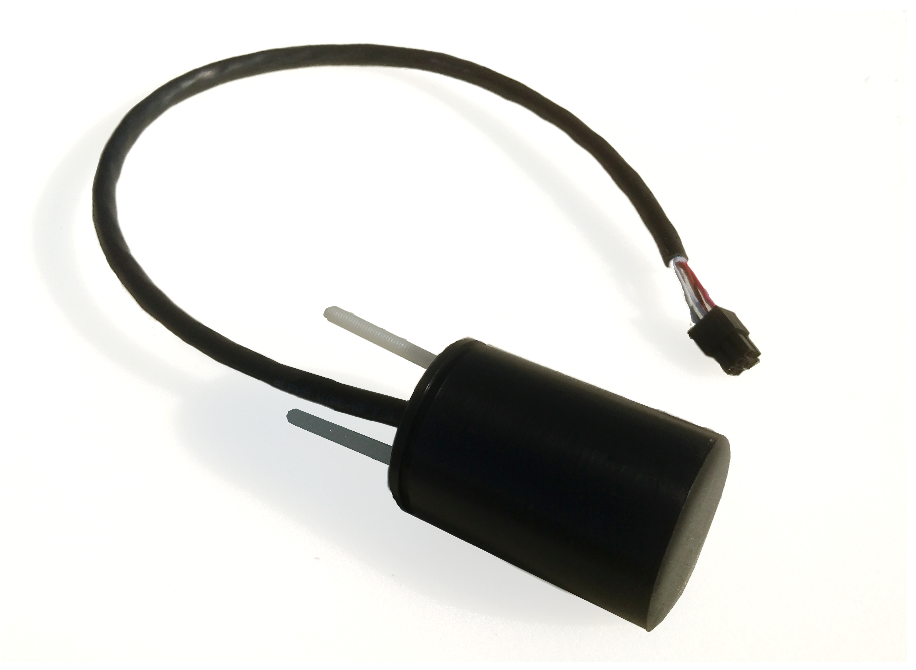
The acoustic modems installed in all members of the swarm are a low-cost miniature acoustic communication and ranging device for underwater vehicles, divers, and subsea instruments developed in Intelligent Sensing and Communications research group at the University of Newcastle, shown in
Figure 3. Communication with the modems is achieved using chirp signal modulation in the 24–28 kHz frequency range, allowing for short data messages of up to 7 bytes to be exchanged between units at a transfer rate of 40 bits per second. Furthermore, an efficient “ping” protocol is implemented for two-way travel time range measurement between units. The farthest distance the communication was successfully established was around 500 m.
Additionally, the acoustic modems have a submodule for acquiring information about the moment of arrival and successful reception of an acoustic packet. The former is useful for acquiring time difference of arrival (TDoA) measurements, and the latter for waking the aMussel up from a low-powered sleep state.
Since the underwater sensor nodes are power limited, there is a significant motivation for implementing energy sharing technologies. The aMussel possesses inductive charging coils which enable battery recharging during mission execution. Together with the low-powered sleep modes mentioned earlier, this can significantly prolong the autonomy of the sensor network.
Wireless energy transfer is realised using a system based on inductive charging [
10,
11], consisting of a power supply on the transmitter side, a set for wireless energy transfer, a battery charger, and a battery. The used wireless charging set is shown in
Figure 4. It consists of a transmitter coil, connected to the appropriate printed circuit board (PCB), which is connected to the power supply and receiver coil connected to the PCB, which is connected to the aMussel battery charger.
The aMussel itself houses two batteries and two independent battery chargers. The primary battery is charged from two wireless receiver coils, while the secondary battery is charged from one wireless charging coil. Charging stops when the wireless receiver stops transferring energy to the chargers or when batteries are full. Monitoring of the charging process is accomplished by tracking the voltages and the currents of the batteries, as well as the digital status pins of each battery.
2.1.2. Actuators
A variable buoyancy system provides the aMussel with its one degree of freedom of movement. It consists of a chamber of variable volume at the bottom of the aMussel, which makes it possible to increase or decrease the total buoyancy of the robot. The actuator controlling this movement is a piston covered with an impermeable membrane, shown in
Figure 5. The volume and the buoyancy of the aMussel are largest when the piston is completely pushed out. In the case where the piston is completely retracted, the aMussel has the smallest volume and the smallest buoyancy. Zero buoyancy is set (using weights) to be somewhere in between, enabling the aMussel to float when the piston is out and to sink when the piston is in. The movement of the piston is accomplished by three electric motors working in tandem, with an incremental encoder present for control purposes. The buoyancy system and the aMussel itself are designed for depths up to 20 m.
2.1.3. Sensors
In line with its primary sensing role, the aMussel is equipped with a variety of sensors capable of monitoring different environmental variables. A sensor for measuring water turbidity and the amount of ambient light is mounted on the aMussel top cap. The top cap also contains a temperature sensor and a pressure sensor used for measuring depth. The aMussel is also equipped with an inertial measurement unit (IMU) located in the top section. The acrylic glass middle section of the aMussel contains a camera with LED lights capable of taking photographs while the aMussel is on the seabed. An additional feature of the aMussel is the electric sense (e-sense) which can serve as a proximity sensor for objects of various materials and shapes, as described in [
12]. The swarm contains several units equipped with sensors for detecting dissolved oxygen. While on the surface, the aMussel can determine its position using its GPS system. This system is also used for clock synchronisation.
2.2. aPad
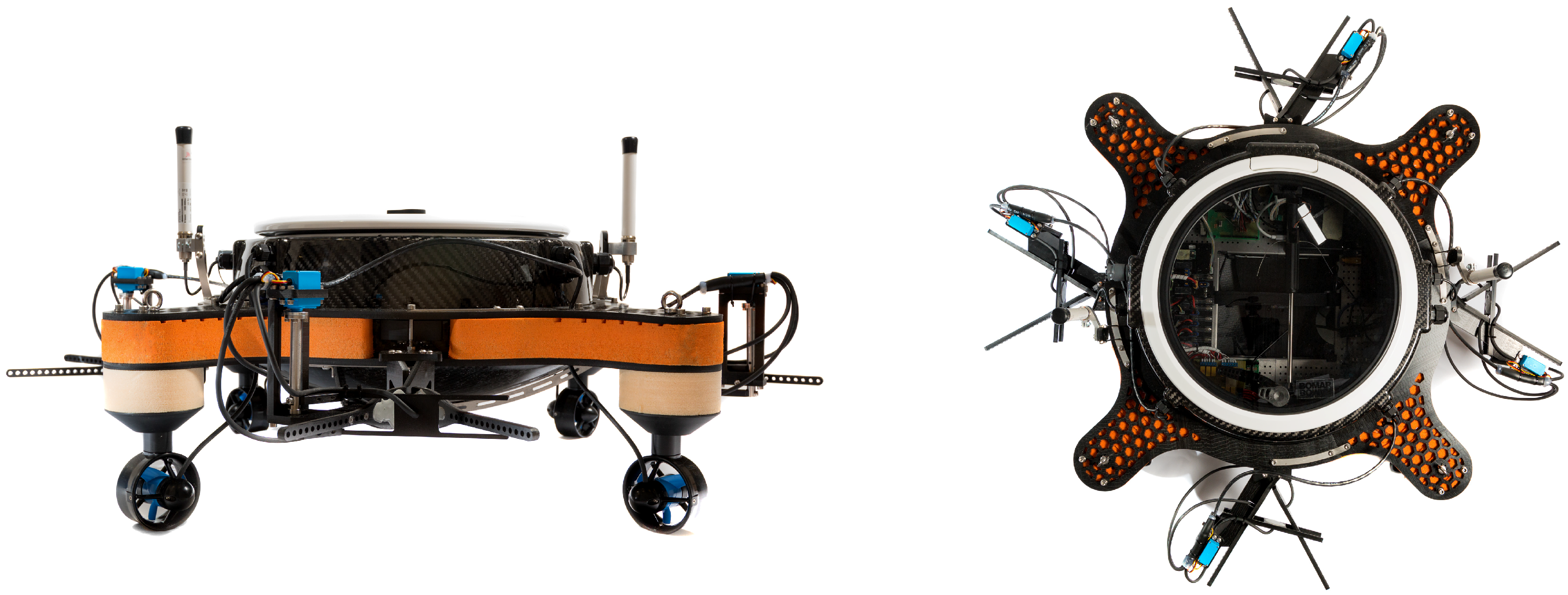
The aPad, shown in
Figure 6, is an overactuated Autonomous Surface Vehicle (ASV). The role of each of the five aPad units present in the subCULTron swarm is that of an energy and information sharing hub. They provide a connection to the terrestrial world—a bridge between the robotic ecosystem and a potential human observer and operator—as well as computational power. They also serve as anchors in the process of underwater localisation.
Equipped with specially developed mechanical docking stations and inductive charging coils, each aPad has the ability to transport and charge up to four aMussels in parallel.
Additionally, the aPads need to be able to adapt to a changing realistic marine environment (
Figure 7), both fighting and exploiting the influence of phenomena such as water currents and wind. One of the energy-efficient aPad behaviours being explored in the system, adapting to changes in their environment even when in a mostly idle state (i.e., not actively performing tasks), is outlined in [
13].
2.2.1. Modules
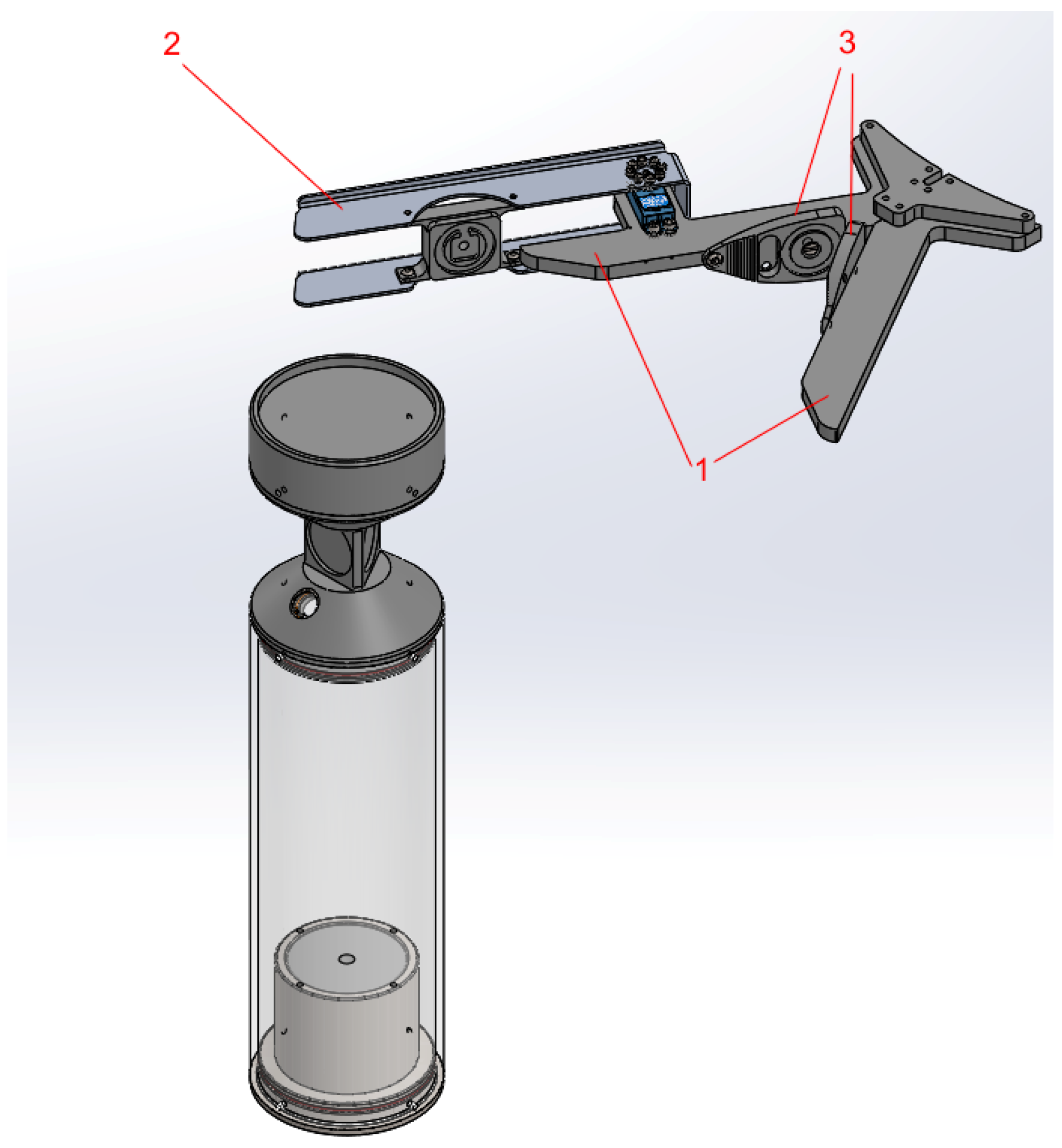
The aPad is equipped with a docking mechanism realised as a mechanical lever system which forces the aMussel into a funnel-shaped slot, as seen in
Figure 8. The aMussel itself has a specially designed docking section shaped as two inverted cones to provide some tolerance for vertical displacement to the docking mechanism and also provide levelling with the charging dock while being forced with the motorised shutter.
The charging dock contains three charging coils encapsulated in waterproof resin which provide wireless energy transfer, and is also shaped in a way to provide tolerance in vertical aMussel angle at approach, as well as mechanical locking once the aMussel is in the slot. The docking principle is purely mechanical with quite high tolerances to offsets with the approaching aMussel, including vertical shift tolerance of mm, and horizontal shift tolerance of mm.
For surface communication purposes, the aPads are equipped with an Ubiquiti UniFi Mesh wireless router. The router operates on two different frequency bands (2.4 GHz and 5 GHz) using a separate antenna for each.
For underwater communication purposes, the aPads contain acoustic modems identical to the ones installed in each aMussel.
2.2.2. Actuators
The aPad has four thrusters in an X-shaped configuration (
Figure 9) which give it significant freedom of movement (in contrast to the aMussel, with regards to actuators limited entirely to its buoyancy system). The platform is capable of omnidirectional movement, and is overactuated.
More on aPad guidance and control is given in
Section 4.1.
2.2.3. Sensors
For localisation and positioning, the aPad uses an IMU and a u-blox C94-M8P GPS module with the capability of using the Real-time kinematic (RTK) positioning technique. This technique can greatly enhance the precision of satellite-based position data using signals from a reference station positioned at a known location. In the absence of the reference station, it acts like a classical GPS unit.
As part of its docking system, the aPad uses both the infra-red and the RGB camera capabilities of the Microsoft Kinect sensor. The Kinect sensor is mounted on the top of the aPad in a sealed vertical tube set upon a servo motor powered pan mechanism. Using the pan mechanism, the Kinect can turn up to 270 degrees, thus offering view on all four aPad docking stations. This setup is shown in
Figure 10.
The aPad has a voltage and current sensor on its power management board which provides information about the vehicle’s battery state.
3. Communication
Communication plays a crucial role in swarms due to multiple factors. No advanced swarm behaviour is possible without communication among the swarm members, both those belonging to the same species and those of different species. Furthermore, monitoring systems utilise synchronous reporting about the state of the environment, asynchronously reporting about occurring events, or offloading measured sensor data to a data hub. Specifically, within the subCULTron swarm, the aMussels periodically report on the current status of the underwater environment, notify other agents if an event has occurred, and transfer collected sensor data to aPads after they surface. These features require the aMussels to be capable of information exchange both while submerged and on the water surface. Communication in the swarm can be split into two categories: surface and underwater communication.
3.1. Surface Wireless Communication
Primary surface information exchange between aPads and aMussels is based on WiFi communication. Since the goal of the system is long-term monitoring, robustness plays a key role in maintaining the usability of the system. Usually, WiFi communication is set up in an Access Point—Client configuration, meaning that several clients connect to one available access point. This introduces a single point of failure in which surface communication in the swarm could fail if the access point were to stop working. Additionally, in order to communicate over WiFi, all agents would need to be in the communication range of the single access point, thus reducing the operating area of the monitoring system.
For these reasons a decentralised approach to mobile networking using a wireless mesh network (WMN) solution was chosen and implemented. WMN is a form of wireless ad-hoc network (WANET), meaning that it does not rely on a fixed network infrastructure [
15] such as the aforementioned access points. Instead, it relies on each node in the network routing the network traffic for itself as well as all other nodes.
Custom firmware based on OpenWRT 17.01.04 was implemented on the aPad’s dual-interface WiFi router. OpenWRT is an operating system targeted for embedded devices allowing custom user configuration easily tailored for any application. Since the aMussel does not have the capability of using mesh routing protocols, each aPad is configured to operate as an access point on the 2.4 GHz interface, giving the aMussels access to the network. Meanwhile, the 5 GHz interface is kept separate and reserved for mesh routing for the aPads, providing better throughput. All traffic between agents which are not connected to the same access point needs to be routed over the mesh interface. The implemented network topology is shown in
Figure 11.
Routing—specifying how wireless routers communicate and establish routes that packets take on their way to their destination—is governed by the mesh routing protocol, and the implementation used on the aPad is open80211s, chosen by analysing the results of authors in [
16]. With a smaller mesh network size as present here with only five aPad nodes, the proposed routing protocol noticeably outperforms similar routing protocols.
3.2. Underwater Acoustic Communication
Currently, the only truly viable option for long range underwater communication is using acoustic signals. Other types of signals used in terrestrial networking rely on electromagnetic waves of high frequency which attenuate rapidly in water [
3]. While greatly increasing the range of communication, the drawbacks of using acoustic communication are low data throughput, large delays in packet delivery, and high probability of transfer failure. These issues are due to the relatively low bandwidth of the signal, slow propagation of sound through water, and a high chance of signal multipath and attenuation.
Successful acoustic communication within a swarm of robots is much more complex than merely supplying them with acoustic modems. Since water is the transmission medium through which all signals propagate during acoustic transmission, collisions can occur during data transfer attempts if two or more agents try to communicate at the same time. To prevent signal collision issues and allow successful communication between all agents sharing the same transmission medium, a communication protocol was developed and implemented.
Multiple access methods are generally divided into the following categories [
17]: frequency division multiple access (FDMA), time division multiple access (TDMA), and code division multiple access (CDMA). Due to the limited capabilities of the acoustic modem used in the swarm, implementing a TDMA-based communication protocol is the only viable option. TDMA allows multiple agents to share the same frequency channel by dividing the signal into different time slots. Each agent can send data to other agents or request data from them within its assigned time slot.
Several different modes of communication were implemented in order to provide the best possible utilisation of the available communication system. The communication protocol was modelled as a finite-state machine (FSM), where each state represents one mode of acoustic communication, shown in
Figure 12.
3.2.1. Scheduling Modes
Since aPads are on the surface and thus easily accessible via wireless communication, they act as masters in acoustic communication by initiating transitions between the FSM states-communication modes. There are four modes of communication: Setup, Default, Priority, and Localisation.
When working with underwater acoustic networks in a real-world experimental environment, the deployment of the system is equally as important as the monitoring phase. None of the sensors should start broadcasting data over the acoustic channel while the system is still in the deployment state, nor should they broadcast if changes are made to the configuration of the sensor network. The first mode of communication addresses this issue by silencing all scheduled communication. In Setup mode, only surface vehicles are allowed to broadcast data or commands. No time scheduling is implemented, and it is the operator’s task not to send commands over the acoustic channel from multiple surface vehicles at the same time. None of the underwater vehicles may initiate communication, but they can respond to requests issued by surface vehicles. This mode achieves the fastest response time from underwater vehicles, which can be useful for issuing urgent commands or reconfiguring the system parameters of the swarm.
In the Default mode, time scheduling is configured using the widely-used round-robin principle [
18]. Time slots are assigned equally among all agents in a circular order, handling communication without priority as can be seen from
Figure 13a. This is the main operating communication mode. Each of the agents in the swarm has an equal amount of time for data sharing, which is well suited to periodically reporting a desired measured environmental variable, for example, monitoring the value of water temperature in the area of deployment.
During mission execution in a real-world environment, it is sometimes desirable for surface agents to issue commands to the underwater agents. A Priority mode was added, in which time slots alternate between each distinctive group of agents by using the round-robin approach, meaning time slots of all aPads and time slots of all aMussels alternate. Within the time slots of each respective group, each individual agent is again scheduled via the round-robin approach. An example of time slot order in this communication mode can be seen in
Figure 13b.
Finally, in the Localisation mode all underwater vehicles are silent and are listening for localisation messages sent from the surface vehicles, i.e., anchors. Time scheduling is implemented using the round-robin principle and is shown in
Figure 13c.
3.2.2. Clock Synchronisation
One of the drawbacks of using TDMA is that great importance must be placed on clock synchronisation. Due to clocks drifting over time, synchronisation needs to be re-executed periodically. Clock synchronisation between aPads is a trivial problem, since they are all on the surface and can easily use their GPS sensor to provide sufficient time precision at any time during mission execution. While the aMussels also have a GPS sensor, they do not have access to GPS signal for most of their deployment as they are underwater.
The RTC module on the aMussel has a time accuracy of ppm, meaning that the clock drift is within s per day. Due to increased energy consumption, it is not a viable solution for aMussels to periodically surface to synchronise their clocks. Initial synchronisation at the time of deployment may be performed via GPS signal, but each subsequent synchronisation is executed using acoustic signals from aPads.
To achieve clock synchronisation via acoustic signal from surface agents, one of the aPads transmits the clock synchronisation sequence containing current epoch time over the acoustic channel. Each of the aMussels on the receiving end stores the time into its RTC after adding known message transmission time . If the area of deployment is constricted to be within the range of a single aPad’s acoustic signal (≈500 m), the worst clock offset of an aMussel is equal to maximal signal propagation time s.
3.2.3. Time Slot Size
The size of communication time slots can be defined during the transition to a specific state of the time scheduling state machine. For selecting time slot size to ensure successful communication with prevention of collisions between transmissions, multiple factors should be taken into account. The most influential factors are the longest message transmission time , maximal signal propagation time based on the range of the acoustic modem , clock synchronisation offset , maximum allowed clock drift time , and guard time . Maximum allowed clock drift time is determined by the RTC module specifications and rate of periodical clock synchronisation. Guard time is defined as a constant and serves to separate subsequent slots in the case of uncertainties in signal propagation time.
Communication between agents can be divided into two categories: data transmission, which requires no response, and data exchange, which requires a response. The longest duration of a single transmission will belong to the second category. The time slot of the agent must therefore be capable of accommodating two longest message transmission times
, a round-trip time based on the range of the modem
, one worst case clock synchronisation offset equal to
, and a guard time of
. This leads to a minimal time slot size for elimination of collisions between transmissions given by:
Since the time slot is large enough for two data transmissions, if an agent does not require a response from the receiving end—such as an aMussel reporting on the status of an environmental variable—it can send twice the amount of data within its timeslot.
Expected time necessary for completing the transmission can be calculated for each specific transmission or exchange, which is useful for determining when in the agent’s time slot a message can be sent. If the time left in the current time slot is shorter than the expected completion time, the message needs to be sent queued up for sending in the next time slot.
The longest single message that can be sent using the equipped acoustic modem is 7 bytes long. The transmission time of a message is defined by
and is heavily dependent on message size. Minimal time slot size with a guard time of
s calculated using (
1) is
s. Since minimal time slot size is calculated based on a worst case scenario, more consideration while choosing time slot size may improve acoustic channel utilisation. For example, the choice of time slot size may be approached statistically by determining the mean value of message size being sent using usual communication patterns while deployed. While time slot size cannot be shortened without making the longest messages cause transmission collision, it can be expanded to better accommodate multiple shorter messages.
4. Agent Capabilities
In this section agent capabilities and functionalities required for successful swarm collaboration are described. The more complex capabilities of the swarm achieved through interaction are also presented. The dependencies of these capabilities on the more basic functionalities of the swarm are shown in
Table 2.
4.1. Guidance and Control
A detailed examination and explanation of the dynamic and kinematic models of the platform, as well as developed low-level control structures, are given in ([
14]). A brief overview is given here for completeness.
The dynamic model of the platform in the horizontal plane can be described using a velocity vector and a vector of actuating forces and moments acting on the platform.
The velocity vector is given by where u, v and r are surge, sway and yaw speed, respectively.
The vector of actuating forces and moments acting on the platform is given by where X, Y are surge and sway forces and N is yaw moment. Both of these vectors are defined in the body–fixed (mobile) coordinate frame.
The platform is designed to be symmetrical with respect to the
x and
y axes in the body-fixed frame. Thus, the uncoupled dynamic model in the horizontal plane is given with (
2) where
is a diagonal matrix with mass and added mass terms for each component expressed with
, and
is a diagonal matrix consisting of nonlinear hydrodynamic damping terms, component-wise
.
The kinematic translatory equations for the platform motion in the horizontal plane on the sea surface are given with (
3), where
x and
y are the position and
is the orientation of the platform in the Earth–fixed coordinate frame and
is the rotation matrix.
An additional equation present in the kinematic model is . The platform is overactuated, i.e., it can move in any direction in the horizontal plane by modifying its surge and sway speed, while attaining arbitrary orientation.
For the low–level speed controller on the aPad, a PI controller was chosen, given with (
4), where
are the desired linear and angular speeds of the platform,
and
are diagonal matrices with proportional and integral gains for individual degrees of freedom, respectively.
The tilde sign marks estimated values—the vehicle’s speeds are often estimated since they are either difficult to measure or any available measurements are fairly unreliable. The
term represents additional action introduced in the controller to improve the closed loop behaviour [
19]. This action can be in the form
which results in the feedback linearisation procedure, in which measured or estimated speeds are used to compensate for the nonlinearity in the process. It is more usual and convenient to use the feedforward term
. Controller parameters
and
can be calculated based on the desired closed loop characteristic equation as shown in [
19].
Notable higher-level control primitives used by the aPads include a go to point manoeuvre and dynamic positioning for station keeping.
4.2. Depth Control
In order to take various measurements at different depths, there is a need for the aMussel to be capable of holding a set depth for a certain amount of time. For this reason, a method for controlling the aMussel depth based on readings from the pressure sensor was implemented. Pressure
p on an object at depth
in a fluid with density
is defined with the following well-known formula:
where
is atmospheric pressure and
g is the gravitational constant. The water density
depends on different factors including temperature and salinity which can be seen in
Figure 14, but since its value in normal conditions will be around
, we have assumed that 1 mbar corresponds to 1 cm of depth.
The aMussel buoyancy system has been modelled as a triple integrator:
where
is depth
,
is velocity
,
is acceleration
,
u is motor PWM reference and
k is a constant. To control the system, a state feedback controller designed using Ackermann’s pole placement formula is used. aMussel depth control responses are shown in
Figure 15, where it can be seen that the aMussel is capable of controlling its depth with the accuracy of a few centimetres, which is more than accurate enough for most applications. Further details about aMussel buoyancy modelling and depth control are given in [
20].
4.3. Underwater Data Acquisition
One of the uses for the aMussel underwater robot, as an example of fusion of perception and movement, is sea environment monitoring. A set of experiments conducted in realistic conditions in Biograd na Moru, Croatia is presented here as an example of some advantages inherent in the robot.
The experiment procedure after the aMussel has been released into the sea is as follows:
Sink to the bottom
Take sensor measurements every 10 s
Surface after 10 min
Turn on GPS
Transfer data to raspberry Pi
Take sensor measurements every 10 s
After 10 min turn off GPS and go back to step 1
When the aMussel is on the surface it is floating freely, carried by the sea currents, while during its time on the bottom the aMussel holds its position.
Figure 16 shows the path of the aMussel recorded by its GPS and shown on Google Earth [
21]. From this figure it can be seen that the sea currents far from the coast are different than the currents when the aMussel is close to the coast.
Figure 17 shows pressure and temperature responses during the experiments, making it possible to observe the water temperature in each individual location where the aMussel sank to the bottom.
Figure 18 shows responses of the aMussel accelerometer and gyroscope, which show that it is possible to register and classify waves when the aMussel is on the surface.
4.4. Docking and Energy Sharing
Once an aMussel has completed a part of its monitoring mission, it surfaces and requests recharging from the aPads.
A detailed description of mechanical modules and algorithms developed for the purpose of enabling energy sharing between two types of robotic agents, as well as an account of experimental procedures used to test the implemented system, is given in [
22].
Autonomous docking is achieved by having the aPad search for and track the top cap of the aMussel using visual servoing and a rotating Kinect sensor looking down on the chosen unoccupied docking unit. The aMussel top cap has been covered in bright red IR reflective tape, enabling use of both RGB and infra-red capabilities of the Kinect sensor. This makes it possible for docking to occur in a wide variety of lighting conditions.
The Kinect image processing algorithm first crops the image to a fixed “horizon” distance, in order to preserve a region of interest where the aMussel might actually be located, thus minimising the chances of false positive detections. Currently, the aPad is capable of observing objects within a radius of 4 m. The algorithm in RGB camera mode uses colour thresholding in the HSV colour space, after applying Contrast-limited Adaptive Histogram Equalization (CLAHE) to the cropped image in order to improve robustness of detection in varying conditions [
23,
24]. In IR camera mode, greyscale thresholding is used. A comparison of a raw and a processed Kinect RGB camera image is given in
Figure 19.
A bounding box is placed around the largest cluster of pixels remaining in the image after thresholding. Visual servoing is accomplished by passing the coordinates of this bounding box to the controller, with the assumption that the origin of the coordinate system is in the centre of the image, both vertically and horizontally. Coordinates are scaled to a range of [−1, 1] for aPad yaw and surge speed control purposes, with −1 corresponding to the left edge and bottom of the image, and 1 being the right edge and top.
A state machine representation of the high-level control of the aPad docking algorithm is given in
Figure 20.
The aPad docking control algorithm loop consists of three active phases:
Search—The aPad rotates at a set rate until it registers a camera frame containing the top cap of an aMussel.
Approach—The aPad moves towards the detected aMussel, turning in order to keep it centered in view and thus properly aligned with the mechanism for docking. Should the aMussel be lost from view during this phase, the aPad will recommence Search.
Grasp—The aPad closes the servo-actuated gripper on its docking mechanism once the reported position of the aMussel is close enough, i.e., below the set height threshold. Charging is started.
The gripper on the docking mechanism is closed once the y coordinate of the located top cap falls below a certain vertical threshold, indicating that the mussel is close to the camera—and the docking point underneath it. This value has been calibrated with regards to the camera angle and the buoyancy and height of the fully surfaced aMussel in order to ensure a timely closing.
The docking and charging setup was tested both in indoor testbeds as well as outside in real-world conditions. Charging status and current measured from both batteries present in the aMussel for the duration of one experiment are shown in
Figure 21.
Negative measured current signifies that the battery is receiving charge, making the start and end of charging easily visible in the resulting plots. Charging status is an indicator which is reported as 0 when there is no charging, and 1 when charging is happening. As expected, the measured current jumps into positive values as soon as charging is stopped. As noted earlier, primary battery A receives more charge than backup battery B (its current measurements reach larger negative values: −750 mA average as opposed to −300 mA average), since it is connected to two of the three inductive coils.
Should the aMussel not need charging, but merely desires to be moved to another location, it will request assistance from a nearby aPad and the docking procedure will happen as described, with the only difference being the aPad not activating its inductive charging coils.
Undocking, or deployment of aMussels, is done simply by the aPad opening the motorised arm of the appropriate dock when it has reached the desired position and moved for several seconds in the opposite direction of the one the chosen dock is facing. This will allow the aMussel to slip out of the docking mechanism even in unfavourable circumstances such as a strong water current hindering its movement, and will put space between the aPad and the now free-floating aMussel. Thus, the aMussel can once again sink to the seabed to continue its measurements, and the aPad can proceed with its other tasks.
5. Swarm Behaviours
Previous sections dealt with describing functionalities and capabilities of the swarm which are not dependent on any type of collective decision making. In order to demonstrate swarm behaviour by executing collaborative tasks, algorithms dependent on information exchange and collective decision making are presented in this section.
5.1. Formation Control
As the developed underwater monitoring system is used for data collection or the detection of underwater events, effective interpretation of collected sensor data relies on knowing the positions of all agents in the system while submerged. Therefore, it stands to reason that long-term monitoring system deployment requires an autonomous method of underwater localisation.
As previously mentioned, aPads can be used as a type of localisation anchor within the subCULTron swarm. In underwater sensor localisation, anchors positioned at known locations provide the source of information necessary for the localisation of unlocalised underwater nodes. In range-based types of localisation, unlocalised nodes collect measurements to gather information about the ranges between them and anchors with known positions. Then, using these measurements and simple algorithms such as multilateration, the unknown node positions can be calculated. In the process of underwater node localisation, it is advantageous to ensure proper spatial configuration of the anchors [
25,
26]. For this reason, a formation control algorithm based on achieving information consensus was developed.
The formation control algorithm used in this paper is based on the algorithm proposed in [
13]. The collision avoidance algorithm used virtual force as expressed with (
7) to repel neighbouring vehicles if they were within the repelling radius.
where
is the sum of virtual forces between vehicle
i and other vehicles in its formation,
and
are regulation parameters,
is the Euclidean distance between vehicle
j and
i, and
is the radius of the repelling zone around the vehicle.
is the normalised vector which points from vehicle
i to vehicle
j, the mathematical expression of which is:
where
is the position of a vehicle in the x-y coordinate plane.
The simulation results for formation control experiments without collision avoidance and experiments with collision avoidance added are shown in
Figure 22. Let us say that the largest width of the aPad is not larger than 1 m, which is then defined as the collision radius. For safety reasons, the repelling radius for collision avoidance is set to 2 m. It can be seen from the experiment shown in
Figure 22a that the distance between vehicles falls below 1 m during the rotation of the formation, which means that collision would happen in a real life experiment. In
Figure 22b the same experiment was reproduced with a collision avoidance algorithm added. During the simulation, the distances between vehicles noticeably do not fall below the defined collision radius, instead oscillating around the repelling radius while the vehicles were circling around each other.
In order to quantify results and enable comparison, formation stabilisation time is introduced. Stabilisation time is defined as the time it takes for all errors in desired distances between agents to fall and stay below a threshold of m, called a victory radius, after a change in formation shape reference. This time is heavily dependent on the differences between the original and new formation shape, meaning the distance each agent needs to traverse in order to change formation shape greatly impacts stabilisation time. For that reason, normalised stabilisation time is defined by dividing determined stabilisation time with the longest distance between the starting and ending points of an agent’s trajectory.
While the collisions were mitigated by introducing virtual force as described in [
13], the stabilisation time increased from
s to
s, while normalised stabilisation time increased from
s/m to
s/m. In the case where agents were instructed to rotate the shape of their formation around its centre by
, the formation control algorithm generated velocity signals to achieve the shortest path to the destination. Subsequently, the superposition of forces generated by the collision avoidance algorithm acted in the opposite direction, leading to oscillations in agent movement visible in
Figure 22b. In other words, when the formation control algorithm set a vehicle velocity which would have caused the agents to collide, the collision avoidance algorithm generated velocity in the opposite direction. Hence a modification of the virtual force formula to generate additional force perpendicular to the repelling force is proposed. With this addition, collision avoidance favours left-hand vehicle passing and situations where the system is stuck oscillating are avoided. The following vector is introduced:
where
is a rotation matrix (
9) providing counterclockwise rotation by 90° used in generating the perpendicular vector.
The proposed modified virtual force replaces
with
, resulting in the following expression:
Using the same starting conditions and formation shape reference as in the previous simulations, experiments were reproduced using the modified collision avoidance algorithm and the results are shown in
Figure 23. The modification to the algorithm reduced the aforementioned oscillations, shortening normalised stabilisation time to
s/m and making it closer in performance to results using the formation control algorithm without collision avoidance. In the following section, experimental results acquired using formation control with the modified collision avoidance algorithm on real vehicles will be presented.
Experimental Results and Discussion
Experimental results collected during field trials in Biograd na Moru, Croatia using three vehicles are shown in
Figure 24.
Figure 24a shows a decrease in normalised stabilisation time in comparison to simulations using the same algorithm, as well as an overall reduction in oscillatory behaviour. During the experiment, the aPads did not collide with each other as distances between them did not fall below the collision radius.
Figure 24b shows a differently shaped formation rotating around its centre by
. Stabilisation time increased to
s from the
s shown in
Figure 24a, but normalised stabilisation time was smaller at
s/m compared to
s/m. These results validate the simulation results and the feasibility of using the formation control algorithm on actual vehicles in a real life environment.
Additionally, experiments with four vehicles were conducted. The results of the experiments using different formation shape references are shown in
Figure 25. The task given was the rotation of a four vehicle formation around its centre by
. The results show noisier position measurements compared to previous experiments which negatively impact stabilisation time. For the experiment in
Figure 25a, stabilisation time and normalised stabilisation time are
s and
s/m respectively. Increasing the victory radius to 1 m (as opposed to the originally selected
m) helps compensate for the higher position noise present in the four vehicle system and leads to the stabilisation time and normalised stabilisation time being reduced to
s and
/m respectively. For the experiment in
Figure 25b, stabilisation time and normalised stabilisation time are
s and
s/m respectively. For the larger victory radius of 1 m, the stabilisation time and normalised stabilisation time were
s and
/m respectively. The results of the experiments with four vehicles show a better normalised stabilisation time compared to earlier experiments with three vehicles, but this is mostly due to the collision avoidance algorithm not needing to intervene as much during the chosen rotation of the formation.
The demonstrated results validate the feasibility of the formation control algorithm successfully controlling the formation shape of four vehicles in a real life environment. A video of the real life experiments can be found at the following link:
https://www.youtube.com/watch?v=-HOWM5OUVXA.
Table 3 shows a summary of results collected in simulation and real life experiments. It can be seen that normalised stabilisation time decreased in real life experiments using three vehicles compared to simulation experiments using three vehicles, which may be due to errors in the estimation of the aPad control model.
5.2. Information Consensus
There are many decisions aMussels will have to make during their operation, such as identifying sensor failures, dividing into subgroups, and managing their energy balance (deciding when to float up for charging). Since there is a large number of agents making joint decisions, one algorithm type that has been considered for their resolution is the well-known consensus algorithms.
Consensus algorithms in the control of multi-agent systems are particularly compelling for their simplicity and a wide range of applications. The foundation of consensus protocols in multi-agent systems lies in the field of distributed computing. In networks of agents,
consensus means to “reach an agreement regarding a certain quantity of interest that depends on the state of all agents” [
27]. A consensus algorithm (protocol) is a series of rules that define information exchange between an agent and all of its neighbours in the network.
Recently, there has been a surge of interest among scientists from different fields in problems related to consensus in networked multi-agent systems. Some of the most interesting problems include the collective behaviour of flocks and swarms [
28], formation control for MRS [
29], optimisation-based cooperative control [
30], sensor fusion [
31], synchronisation of coupled oscillators, asynchronous distributed algorithms, and many more.
However, there have not been many advancements in the area of underwater consensus protocols. To the best of the authors’ knowledge, the only underwater consensus applications include formation control of tethered and untethered underwater vehicles [
32,
33,
34] and tracking of underwater targets using acoustic sensor networks (ASN) [
35]. Both of those approaches have been validated only in the simulation environment, using ideal communication channels.
In the subCULTron swarm application, the problem of operation under the conditions of poor communication is tackled. Although each aMussel has two underwater communication devices—green light and acoustic modem—only the latter and its implications on consensus algorithms is considered. Other considerations of application of consensus algorithms to the swarm have been presented in the authors’ previous works [
36,
37], but are beyond the scope of this paper.
5.2.1. Consensus Protocol for Sequenced Communication
A distributed system of
n integrator agents with dynamics
is being considered, where
represents agent
i’s state, whereas
is the control input. The goal of consensus protocols, in general, is to design a control algorithm that enables agents to reach a homogeneous stationary state
, that is,
State variables
can correspond to some physical property. Initial states of all agents are represented by a vector
.
Agents update their values based on the information exchanged via local communication with their neighbours. The underlying communication graph is defined as with the set of nodes and edges .
An iterative form of the discrete-time consensus algorithm for reaching the average value of
n integrator agents [
27] is stated as follows:
where
k and
denote discrete time steps of the algorithm, and
represents a set of all nodes adjacent to the
ith node, and
is the step-size.
The collective dynamics of the network under this algorithm can be written as
with
.
I is the identity matrix and
L is known as
graph Laplacian of G. Matrix
L is defined as
where
is the degree matrix of
G with elements
and zero off-diagonal elements.
is the adjacency matrix of the graph G.
The consensus algorithm (
12) assumes synchronous information exchange at every time step k with no time delays, and its convergence into the average value of all initial states is mathematically proven [
27]. Although some algorithms take into account systems with delayed and asynchronous communication [
38], there are none to the authors’ knowledge that operate under the scheduled sequenced communication. The following algorithm has been developed in [
39] and is in short outlined below.
The described behaviour is modelled through manipulating the Laplacian matrix to switch the communication topology depending on the current state of the system. The modified Equation (
13) is given by
with
, where
represents the graph Laplacian calculated as
. Both
and
are calculated using a specially devised vector
m used as a
mask of the underlying communication topology. Assuming a communication scheme as defined earlier and round-robin scheduling of time slots in a system of
n agents, elements of vector
are defined as
where
, and
i represents the index of the time slot. Each change of the vector
m triggers the execution of the algorithm described with (
15). Degree and adjacency matrices are defined as
5.2.2. Experimental Results
A series of experiments was conducted on a real system of four aMussel robots in the Venetian Arsenal. All robots are equipped with acoustic communication devices. The optimal period of message transmission was empirically defined to be . Smaller periods have displayed interference in the signals. Moreover, having a somewhat longer communication period ensures correctness of each transmission even after a slight drift in the robots’ clocks.
The initial values of the variable states and the expected stationary state were set to
and
, respectively. The gain was set to
. The results are provided in
Figure 26. As is seen in the graph, the values converge to 110 after
of the experiment runtime.
6. Conclusions
In this paper an implementation of a heterogeneous robotic swarm designed for long-term autonomous monitoring of marine environments was described. The capabilities and roles of two different agent types were given in detail, as well as the interactions possible between them.
Insight was given into the surface and underwater modes of communication developed for the purpose of allowing the swarm to engage in advanced behaviours. On the surface, a dual network topology consisting of a mesh network and a system of access points was implemented. In underwater communication, inexpensive acoustic modems have proven to be reliable in providing necessary information exchange during experiments by following an acoustic communication protocol based on Time Division Multiple Access. Individual and collaborative capabilities of the robotic swarm were demonstrated through experiments in real-world environments and conditions.
As part of the further development of the swarm, advanced underwater localisation algorithms will be implemented. The scalability of current algorithms and behaviours will be extensively tested. High-level evolutionary decision-making, task allocation, and scheduling algorithms will be incorporated into the swarm’s collaborative behaviours, increasing the range and efficiency of its autonomous exploration and monitoring capabilities.
Author Contributions
Conceptualisation, N.M., S.B. and T.P.; Methodology, A.B., B.A., G.V. and I.L.; Software, A.B., B.A., G.V., I.L. and T.P.; Validation, A.B., B.A., G.V. and I.L.; Formal analysis, A.B., B.A., G.V. and I.L.; Supervision, N.M., S.B. and T.P.
Funding
This work was supported in part by the Croatian Science Foundation under Project IP-2016-06-2082 “Cooperative robotics in marine monitoring and exploration” and in part by the European Union through the EU H2020 FET-Proactive project “subCULTron,” No. 640967. The work of doctoral students Barbara Arbanas and Ivan Lončar has been supported in part by the “Young researchers’ career development project—training of doctoral students” of the Croatian Science Foundation funded by the European Union from the European Social Fund.
Acknowledgments
The authors wish to thank the members of the consortium of the project ‘subCULTron’ consisting of Artificial Life Lab—University of Graz, Unit of Social Ecology—Université Libre de Bruxelles, Cybertronica Research, IRCCyN—Ecole des Mines de Nantes, BioRobotics Institute—Scuola Superiore Sant’Anna, CORILA: Consortium for coordination of research activities concerning the Venice lagoon system and ISMAR Istituto di Scienze Marine.
Conflicts of Interest
The authors declare no conflict of interest.
Abbreviations
The following abbreviations are used in this manuscript:
| ASV | Autonomous surface vehicle |
| CDMA | Code-Division Multiple Access |
| FDMA | Frequency-Division Multiple Access |
| FSM | Finite-state machine |
| GPS | Global Positioning System |
| IMU | Inertial measurement unit |
| IR | Infra-red |
| LED | Light emitting diode |
| RTC | Real-time clock |
| RTK | Real-time kinematic |
| TDMA | Time-Division Multiple Access |
| UASN | Underwater acoustic sensor network |
| WANET | Wireless ad-hoc network |
| WMN | Wireless mesh network |
References
- Akyildiz, I.F.; Pompili, D.; Melodia, T. Underwater acoustic sensor networks: Research challenges. Ad Hoc Netw. 2005, 3, 257–279. [Google Scholar] [CrossRef]
- Akyildiz, I.F.; Pompili, D.; Melodia, T. State-of-the-art in Protocol Research for Underwater Acoustic Sensor Networks. In Proceedings of the 1st ACM International Workshop on Underwater Networks, Los Angeles, CA, USA, 25 September 2006; ACM: New York, NY, USA, 2006; pp. 7–16. [Google Scholar] [CrossRef]
- Tan, H.P.; Diamant, R.; Seah, W.K.; Waldmeyer, M. A survey of techniques and challenges in underwater localization. Ocean Eng. 2011, 38, 1663–1676. [Google Scholar] [CrossRef]
- Tuna, G.; Gungor, V.C. A survey on deployment techniques, localization algorithms, and research challenges for underwater acoustic sensor networks. Int. J. Commun. Syst. 2017, 30, e3350. [Google Scholar] [CrossRef]
- Bian, T.; Venkatesan, R.; Li, C. Design and Evaluation of a New Localization Scheme for Underwater Acoustic Sensor Networks. In Proceedings of the GLOBECOM 2009—2009 IEEE Global Telecommunications Conference, Honolulu, HI, USA, 30 November–4 December 2009; pp. 1–5. [Google Scholar] [CrossRef]
- Liu, B.; Chen, H.; Zhong, Z.; Poor, H.V. Asymmetrical Round Trip Based Synchronization-Free Localization in Large-Scale Underwater Sensor Networks. IEEE Trans. Wirel. Commun. 2010, 9, 3532–3542. [Google Scholar] [CrossRef]
- Thenius, R.; Moser, D.; Varughese, J.C.; Kernbach, S.; Kuksin, I.; Kernbach, O.; Kuksina, E.; Mišković, N.; Bogdan, S.; Petrović, T.; et al. subCULTron—Cultural Development as a Tool in Underwater Robotics. In Artificial Life and Intelligent Agents; Lewis, P.R., Headleand, C.J., Battle, S., Ritsos, P.D., Eds.; Springer International Publishing: Cham, Switzerland, 2018; pp. 27–41. [Google Scholar]
- Jaffe, J.S.; Franks, P.J.S.; Roberts, P.L.D.; Mirza, D.; Schurgers, C.; Kastner, R.; Boch, A. A swarm of autonomous miniature underwater robot drifters for exploring submesoscale ocean dynamics. Nat. Commun. 2017, 8, 14189. [Google Scholar] [CrossRef]
- Roemmich, D.; Owens, W.B. The Argo Project: Global ocean observations for understanding and prediction of climate variability. Oceanography 2000, 13, 45–50. [Google Scholar] [CrossRef]
- Kan, T.; Mai, R.; Mercier, P.P.; Mi, C. Design and Analysis of a Three-Phase Wireless Charging System for Lightweight Autonomous Underwater Vehicles. IEEE Trans. Power Electron. 2017, 33, 6622–6632. [Google Scholar] [CrossRef]
- McGinnis, T.; Henze, C.P.; Conroy, K. Inductive Power System for Autonomous Underwater Vehicles. In Proceedings of the OCEANS’07 MTS/IEEE Conference, Vancouver, BC, Canada, 29 September–4 October 2007; pp. 1–5. [Google Scholar] [CrossRef]
- Lebastard, V.; Boyer, F.; Lanneau, S. Reactive underwater object inspection based on artificial electric sense. Bioinspir. Biomim. 2016, 11, 045003. [Google Scholar] [CrossRef]
- Babić, A.; Lončar, I.; Mišković, N.; Vukić, Z. Energy-efficient environmentally adaptive consensus-based formation control with collision avoidance for multi-vehicle systems. IFAC-PapersOnLine 2016, 49, 361–366. [Google Scholar] [CrossRef]
- Nađ, D.; Mišković, N.; Mandić, F. Navigation, guidance and control of an overactuated marine surface vehicle. Annu. Rev. Control 2015, 40, 172–181. [Google Scholar] [CrossRef]
- Han, L. Wireless ad-hoc networks. Wirel. Pers. Commun. J. 2004, 4. Available online: https://pdfs.semanticscholar.org/cbd2/9938dd4cbeb8aec3c21ddb60f0f20a4356cb.pdf (accessed on 2 April 2019).
- Pojda, J.; Wolff, A.; Sbeiti, M.; Wietfeld, C. Performance analysis of mesh routing protocols for UAV swarming applications. In Proceedings of the 2011 8th International Symposium on Wireless Communication Systems, Aachen, Germany, 6–9 November 2011; pp. 317–321. [Google Scholar] [CrossRef]
- Doukkali, H.; Nuaymi, L. Analysis of MAC protocols for underwater acoustic data networks. In Proceedings of the 2005 IEEE 61st Vehicular Technology Conference, Stockholm, Sweden, 30 May–1 June 2005; Volume 2, pp. 1307–1311. [Google Scholar] [CrossRef]
- Miao, G.; Zander, J.; Sung, K.; Slimane, S. Fundamentals of Mobile Data Networks; Cambridge University Press: Cambridge, UK, 2016; pp. 1–304. [Google Scholar] [CrossRef]
- Caccia, M.; Bibuli, M.; Bono, R.; Bruzzone, G. Basic navigation, guidance and control of an Unmanned Surface Vehicle. Auton. Robot. 2008, 25, 349–365. [Google Scholar] [CrossRef]
- Vasiljevic, G.; Arbanas, B.; Bogdan, S. Ambient light based depth control of underwater robotic unit aMussel. In Proceedings of the IEEE International Conference on Robotics and Automation, Montreal, ON, Canada, 20–24 May 2019. accepted. [Google Scholar]
- Google Earth. 2018. Available online: https://www.google.com/earth/ (accessed on 25 October 2018).
- Babić, A.; Mandić, F.; Vasiljević, G.; Mišković, N. Autonomous docking and energy sharing between two types of robotic agents. IFAC-PapersOnLine 2018, 51, 406–411. [Google Scholar] [CrossRef]
- Kumar Rai, R.; Gour, P.; Singh, B. Underwater image segmentation using clahe enhancement and thresholding. Int. J. Emerg. Technol. Adv. Eng. 2012, 2, 118–123. [Google Scholar]
- Reza, A.M. Realization of the Contrast Limited Adaptive Histogram Equalization (CLAHE) for Real-Time Image Enhancement. J. VLSI Signal Process. Syst. Signal Image Video Technol. 2004, 38, 35–44. [Google Scholar] [CrossRef]
- Bishop, A.N.; Fidan, B.; Anderson, B.D.O.; Dogancay, K.; Pathirana, P.N. Optimality Analysis of Sensor-Target Geometries in Passive Localization: Part 1—Bearing-Only Localization. In Proceedings of the 2007 3rd International Conference on Intelligent Sensors, Sensor Networks and Information, Melbourne, Australia, 3–6 Decemebr 2007; pp. 7–12. [Google Scholar] [CrossRef]
- Moreno-Salinas, D.; Pascoal, A.; Aranda, J. Optimal Sensor Placement for Acoustic Underwater Target Positioning with Range-Only Measurements. IEEE J. Ocean. Eng. 2016, 41, 620–643. [Google Scholar] [CrossRef]
- Olfati-Saber, R.; Fax, J.A.; Murray, R.M. Consensus and Cooperation in Networked Multi-Agent Systems. Proc. IEEE 2007, 95, 215–233. [Google Scholar] [CrossRef]
- Olfati-Saber, R.; Jalalkamali, P. Coupled Distributed Estimation and Control for Mobile Sensor Networks. IEEE Trans. Autom. Control 2012, 57, 2609–2614. [Google Scholar] [CrossRef]
- Fax, J.A.; Murray, R.M. Information flow and cooperative control of vehicle formations. IEEE Trans. Autom. Control 2004, 49, 1465–1476. [Google Scholar] [CrossRef]
- Alighanbari, M.; How, J.P. Decentralized Task Assignment for Unmanned Aerial Vehicles. In Proceedings of the 44th IEEE Conference on Decision and Control, Seville, Spain, 12–15 December 2005; pp. 5668–5673. [Google Scholar] [CrossRef]
- Olfati-Saber, R. Distributed Kalman filtering for sensor networks. In Proceedings of the 2007 46th IEEE Conference on Decision and Control, New Orleans, LA, USA, 12–14 December 2007; pp. 5492–5498. [Google Scholar] [CrossRef]
- Joordens, M.A.; Jamshidi, M. Consensus Control for a System of Underwater Swarm Robots. IEEE Syst. J. 2010, 4, 65–73. [Google Scholar] [CrossRef]
- Putranti, V.; Ismail, Z.H.; Namerikawa, T. Robust-formation control of multi-Autonomous Underwater Vehicles based on consensus algorithm. In Proceedings of the 2016 IEEE Conference on Control Applications (CCA), Buenos Aires, Argentina, 19–22 September 2016; pp. 1250–1255. [Google Scholar]
- Mirzaei, M.; Meskin, N.; Abdollahi, F. Robust distributed consensus of autonomous underwater vehicles in 3D space. In Proceedings of the 2016 International Conference on Control, Decision and Information Technologies (CoDIT), Paris, France, 23–26 April 2016; pp. 399–404. [Google Scholar]
- Yan, J.; Pu, B.; Tian, X.; Luo, X.; Li, X.; Guan, X. Distributed target tracking using consensus-based Bayesian filtering by underwater acoustic sensor networks. In Proceedings of the 2017 36th Chinese Control Conference (CCC), Dalian, China, 26–28 July 2017; pp. 8789–8794. [Google Scholar]
- Arbanas, B.; Petrovic, T.; Bogdan, S. Consensus Protocol for Underwater Multi-Robot System Using Two Communication Channels. In Proceedings of the 2018 26th Mediterranean Conference on Control and Automation (MED), Zadar, Croatia, 19–22 June 2018; pp. 358–363. [Google Scholar]
- Mazdin, P.; Arbanas, B.; Haus, T.; Bogdan, S.; Petrovic, T.; Miskovic, N. Trust Consensus Protocol for Heterogeneous Underwater Robotic Systems. IFAC-PapersOnLine 2016, 49, 341–346. [Google Scholar] [CrossRef]
- Xiao, F.; Wang, L. Asynchronous Consensus in Continuous-Time Multi-Agent Systems with Switching Topology and Time-Varying Delays. IEEE Trans. Autom. Control 2008, 53, 1804–1816. [Google Scholar] [CrossRef]
- Arbanas, B.; Petrovic, T.; Bogdan, S. Consensus Protocol for Underwater Multi-Robot System Using Scheduled Acoustic Communication. In Proceedings of the 2018 OCEANS—MTS/IEEE Kobe Techno-Oceans (OTO), Kobe, Japan, 28–31 May 2018; pp. 1–5. [Google Scholar] [CrossRef]
Figure 1.
subCULTron Underwater Acoustic Sensor Networks (UASN) concept.
Figure 1.
subCULTron Underwater Acoustic Sensor Networks (UASN) concept.
Figure 2.
The aMussel marine robot and underwater sensor node.
Figure 2.
The aMussel marine robot and underwater sensor node.
Figure 3.
Acoustic modem Nanomodem.
Figure 3.
Acoustic modem Nanomodem.
Figure 4.
Wireless charging set.
Figure 4.
Wireless charging set.
Figure 5.
aMussel buoyancy system. Left image shows aMussel with piston completely in, and right shows it with piston completely out.
Figure 5.
aMussel buoyancy system. Left image shows aMussel with piston completely in, and right shows it with piston completely out.
Figure 6.
The artificial lily pad (aPad) autonomous surface platform, front view (left) and top view (right).
Figure 6.
The artificial lily pad (aPad) autonomous surface platform, front view (left) and top view (right).
Figure 7.
Members of the subCULTron swarm operating in real-world conditions, Venice, Italy.
Figure 7.
Members of the subCULTron swarm operating in real-world conditions, Venice, Italy.
Figure 8.
Illustration of docking mechanism mounted on aPad, consisting of two immovable delrin levers (1) mounted on the aPad which act as a guiding rail funnelling the aMussel towards the charging dock, a motorised aluminium shutter (2) that pushes on the aMussel while closing, and a charging dock (3).
Figure 9.
X-shaped thruster configuration present on the aPad, enabling omnidirectional motion in the horizontal plane, [
14].
Figure 9.
X-shaped thruster configuration present on the aPad, enabling omnidirectional motion in the horizontal plane, [
14].
Figure 10.
Kinect sensor and pan mechanism mounted on the aPad platform-design (left) and realisation (right).
Figure 10.
Kinect sensor and pan mechanism mounted on the aPad platform-design (left) and realisation (right).
Figure 11.
Swarm network topology. Green lines represent mesh network traffic routed over the 5 GHz interface, while red lines represent Access Point—Client traffic over the 2.4 GHz interface.
Figure 11.
Swarm network topology. Green lines represent mesh network traffic routed over the 5 GHz interface, while red lines represent Access Point—Client traffic over the 2.4 GHz interface.
Figure 12.
State machine representation of modes of communication.
Figure 12.
State machine representation of modes of communication.
Figure 13.
Time scheduling modes of communication.
Figure 13.
Time scheduling modes of communication.
Figure 14.
Water density depending on water temperature and salinity.
Figure 14.
Water density depending on water temperature and salinity.
Figure 15.
Depth control pressure response.
Figure 15.
Depth control pressure response.
Figure 16.
Floating experiment aMussel path.
Figure 16.
Floating experiment aMussel path.
Figure 17.
Floating experiment aMussel temperature and pressure responses.
Figure 17.
Floating experiment aMussel temperature and pressure responses.
Figure 18.
Floating experiment aMussel inertial measurement unit (IMU) responses for x, y and z component.
Figure 18.
Floating experiment aMussel inertial measurement unit (IMU) responses for x, y and z component.
Figure 19.
Examples of the aPad Kinect RGB image, original (left) and processed (right). The green rectangle superimposed on the camera image represents a bounding box around the derived position of the aMussel top cap used to control the aPad’s approach.
Figure 19.
Examples of the aPad Kinect RGB image, original (left) and processed (right). The green rectangle superimposed on the camera image represents a bounding box around the derived position of the aMussel top cap used to control the aPad’s approach.
Figure 20.
State machine representation of the aPad controller running the docking algorithm.
Figure 20.
State machine representation of the aPad controller running the docking algorithm.
Figure 21.
Battery current and charging status of batteries A (left) and B (right).
Figure 21.
Battery current and charging status of batteries A (left) and B (right).
Figure 22.
Simulation results of rotating a formation around its centre by without (a) and with (b) collision avoidance.
Figure 22.
Simulation results of rotating a formation around its centre by without (a) and with (b) collision avoidance.
Figure 23.
Simulation results of rotating a formation around its centre by with the modified collision avoidance algorithm.
Figure 23.
Simulation results of rotating a formation around its centre by with the modified collision avoidance algorithm.
Figure 24.
Experimental results of rotating a three vehicle formation around its centre by .
Figure 24.
Experimental results of rotating a three vehicle formation around its centre by .
Figure 25.
Experimental results of rotating a four vehicle formation around its centre by .
Figure 25.
Experimental results of rotating a four vehicle formation around its centre by .
Figure 26.
Results of the consensus algorithm applied to four aMussel robots using acoustic communication.
Figure 26.
Results of the consensus algorithm applied to four aMussel robots using acoustic communication.
Table 1.
Swarm capabilities.
Table 1.
Swarm capabilities.
| | | Perception | Information
Exchange | Energy
Sharing | Navigation and
Movement |
|---|
| Modules | Acoustic modem | | ⨂ | | |
| Docking station | | | × | |
| Green Light | | ◯ | | |
| GSM | | ◯ | | |
| Inductive charging | | | ⨂ | |
| WiFi modem | | ⨂ | | |
| Actuators | Buoyancy system | | | | ◯ |
| Propulsion system | | | | × |
| Sensors | Ambient light | ◯ | | | |
| Battery state | ⨂ | | ⨂ | |
| E-Sense | ◯ | | | |
| GPS | ⨂ | | | × |
| IMU | ⨂ | | | ⨂ |
| IR camera | × | | | |
| Oxygen | ◯ | | | |
| Pressure | ◯ | | | ◯ |
| RGB camera | ⨂ | | | |
| RTC | ⨂ | ⨂ | | |
| Temperature | ◯ | | | |
| Turbidity | ◯ | | | |
Table 2.
Swarm interactions.
Table 2.
Swarm interactions.
| | Interactions |
|---|
| | Intraspecies | Interspecies |
|---|
| | Information
Consensus | Formation
Control | Underwater
Localisation | Distributed
Sensing | Sensor Node
Recharging | Sensor Node
Relocation |
|---|
| Perception | ◯ | × | ⨂ | ◯ | ⨂ | ⨂ |
| Information Exchange | ◯ | × | ⨂ | ⨂ | ⨂ | ⨂ |
| Energy sharing | | | | | ⨂ | |
| Navigation and movement | | × | | | × | ⨂ |
Table 3.
Comparison of stabilisation times for conducted simulation and real experiments.
Table 3.
Comparison of stabilisation times for conducted simulation and real experiments.
| | Simulation | Real Experiments |
|---|
| | no CA | CA | modified CA |
|---|
| | 3 Vehicles | 4 Vehicles |
|---|
| Shape | Triangle | Triangle | Triangle | Triangle | Line | Triangle | Square |
| Rotation amount | | | | | | | |
| Stabilisation time (s) | 10.6 | 32.7 | 16.6 | 12.2 | 23.8 | 11.4 | 8.5 |
| Normalised stabilisation time (s/m) | 2.8 | 8.6 | 4.2 | 3.1 | 2.8 | 2.8 | 2.9 |
© 2019 by the authors. Licensee MDPI, Basel, Switzerland. This article is an open access article distributed under the terms and conditions of the Creative Commons Attribution (CC BY) license (http://creativecommons.org/licenses/by/4.0/).

 ,
, 


