High-Precision Light Spot Position Detection in Low SNR Condition Based on Quadrant Detector

Abstract

In free space optical communications, long-distance transmission leads to the attenuation of beacon light, where we adopt a quadrant detector (QD) to receive the weak signal. However, the background light interferes so strongly that the output signal-to-noise ratio (SNR) of QD is at a low level, which causes a decrease in accuracy of the direct detection method. This requires finding a new light spot detection method, so an improved detection method is proposed. Because the dark current noise and the background light noise are both white noise, we adopt a Kalman filter to estimate the real output of four electric signals of QD. Unfortunately, running these through an amplifier introduces some direct current (DC) offsets into the signals. In order to balance the effect of the DC offsets, we consider using the modulation method, where we employ a sine signal to modulate the intensity of the beacon light at the transmitting end, after which we can give an inverse gain to move the center of signals to near zero to eliminate the DC offsets when we calculate the data. In Kalman filtering, we use the peak values of the signals in every period after the analog to digital converter (ADC) as the elements of the measurement matrix. Experimental results show that even when QD output SNR is about −10 dB, the detection root-mean-square errors decrease by 51.5% using the improved detection method compared with the direct detection method. Moreover, Kalman filtering does not require a large amount of data, which means it works efficiently, can reduce the cost of hardware resources, and is available for the real-time calculation of spot position.

1. Introduction

Free space optical (FSO) communication, working as the main mode of satellites to ground communication, has received increasing attention from scientists from all over the world. It is a combination of wireless communication and optical fiber communication, which means it has the advantages of both communication modes to help us realize point-to-point transmission. However, it is not an easy task to keep the transmitting end and the receiving end aimed at and tracking each other [1,2]. The high detecting accuracy of light spot detection can guarantee high performance of FSO systems, which brings us a stable communication link between the satellites end and ground end.

A laser beam of 1550 nm wavelength is widely applied to laser communication systems because it is weakly affected by atmosphere turbulence compared with other laser wavelengths [3]. We usually use a charged coupled device (CCD) as the position feedback device, but the low quantum efficiency of CCD at 1550 nm limits its use [4,5]. This is especially true when the distance between satellites and the ground increases; considering the effect of atmosphere channel, the energy of the beacon light decreases considerably. Here, we apply a quadrant detector (QD) as our detector because of its high resolution, which can help us acquire the signals whose energy are at the nanowatt (nW) level. What is more, its natural noise is low and response speed fast, all of which indicating that it can play the role as the detector of satellites to ground communication well.

Wu and colleagues analyzed the nonlinear characteristics of QD and proposed a linear correction method based on the Boltzmann function [4]. When they received the position of a light spot, it could be calculated by the Boltzmann function, whose parameters were known by experiment. Dang and colleagues analyzed the characteristics of the detector output signal [6]. The estimated spot position values and the real spot position values were calibrated by Chen and colleagues, the calibrated values then fitted to the polynomial [7]. This method is similar to the Boltzmann function method, the main difference being the greater complexity of the function employed in the method proposed by Chen and colleagues.

In a word, the scientists above adopted the direct detection method, which directly detects the amplitude of the output photocurrents of QD to correct the non-linearity. The methods they proposed are used in the situations when the QD output signal is greater than the noise, or almost at the same. That is to say, when the SNR is at a low level, the methods do not work well. Therefore, we propose using a Kalman filter to distinguish the signals from the noise.

However, when the output photocurrents of QD are sent to the amplifiers, some DC offsets are brought into the signal, affecting the values of the useful signals. In order to solve this problem, we suggest using a modulation method, where we use a sine signal to modulate the intensity of the beacon light at the transmitting end, after which we can give an inverse gain to move the center of signals to zero to eliminate the DC offsets before the data are sent to the Kalman filter. After the signals are run through a ADC, we use the peak values of the output signals in every period as the elements of the measurement matrix, which already contains measurement noise. Using the Kalman method can help us filter out the white noise and improve the detecting accuracy. What is more, the method requires few steps of iteration, which helps us to realize real-time processing.

In the following sections of the paper, we first introduce the description of QD characteristics in order to get the output signal form of QD. Then, we compare the working process of the direct detection method with the improved detection method. Finally, we set up an experimental platform to verify the effects of the Kalman filtering method.

2. Description of QD Characteristics

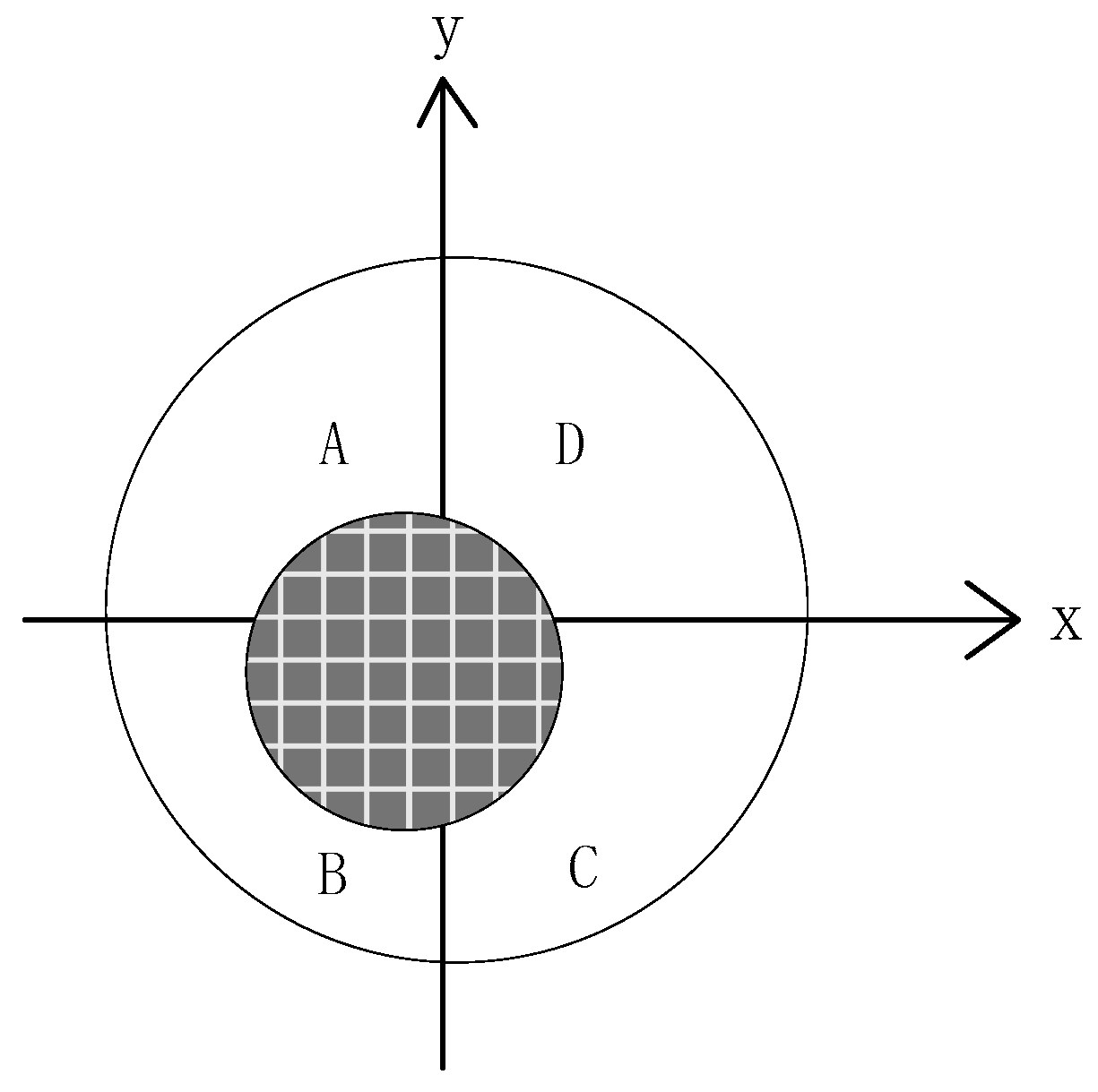
As Figure 1 shows, QD consists of four identical p-n junction photo-diodes, which can turn optical signals into electric signals through the photoelectric effect when a beacon light is received.

The outputs of QD are four electric signals, which are independent of one another, whose amplitude is closely related to the energy of the four parts of the optical signals that illuminate each photo-diode and their transition gain [8]. The photoelectric effect can be expressed as follows.

If the incident light obeys normal distribution, its power density can be written as [9,10]:

$$\overline{p}\left(x,y\right)=\frac{2p_0}{\pi {\omega }^2}\exp \left\{-\frac{2\left[{\left(x-x_0\right)}^2+{\left(y-y_0\right)}^2\right]}{{\omega }^2}\right\}$$

(1)

Here: $\omega$ is the spot radius, $\left(x_0,y_0\right)$ is the coordinate of the spot center, $p_0$ is the power of the incident light, and the center of the QD is the origin of the coordinates.

So in one quadrant, the energy of the light in one second can be written as:

$$E={\displaystyle \underset{S}{\iint }p\left(x,y\right)dxdy}$$

(2)

After the photoelectric effect, optical signals are transformed into photocurrents, which can be expressed as [11]:

$$I=KE=\frac{e\eta }{h\nu }{\displaystyle \underset{S}{\iint }p\left(x,y\right)dxdy}$$

(3)

Here: $K$ is the transition gain of the diode, $e$ is the elementary charge, $\eta$ is the transfer efficiency, $h$ is the planck constant, and $\nu$ is the frequency of the incident light.

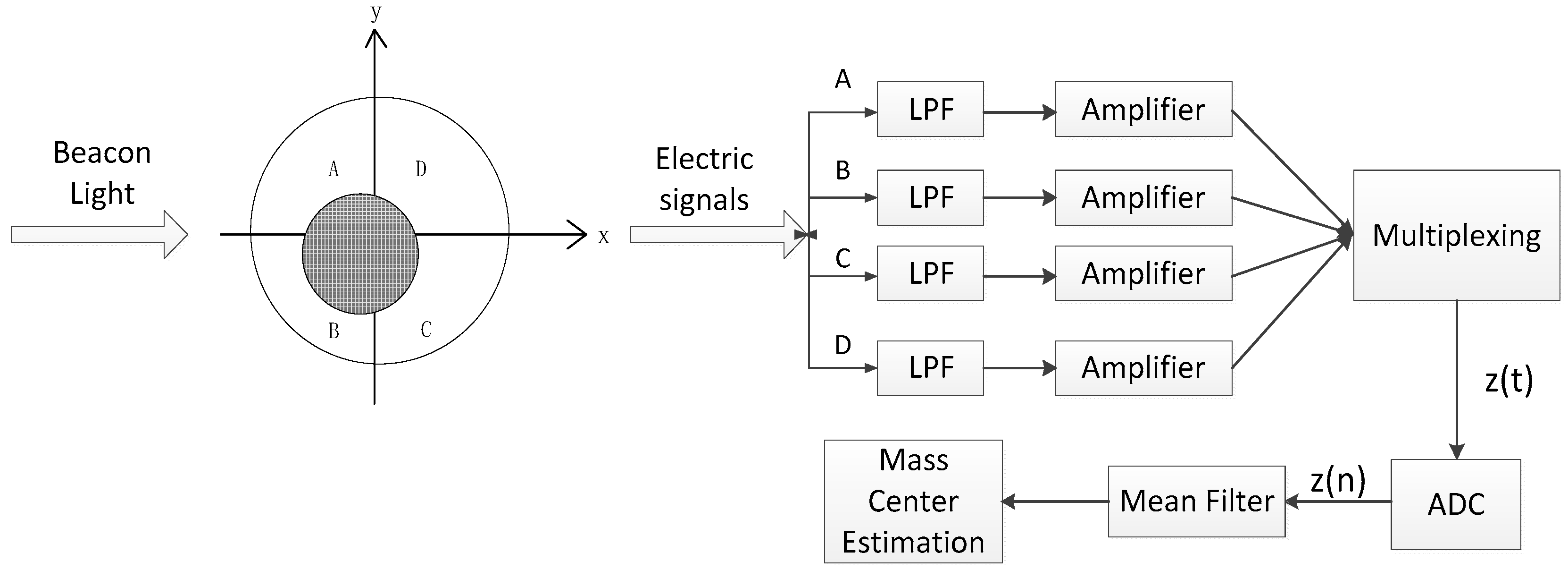
3. Direct Detection Method

The traditional direct detection method, as described previously in References [4,6,7], is shown in Figure 2.

As we can see in Figure 2, the four output electrical signals are sent to low pass filters (LPF) first. Then they pass through amplifiers to increase the amplitudes. After analog to digital conversion, the data are put into a mean filter. Finally, the mass center estimation described as the following expression (4) can calculate the deviation of the light spot.

When the center position of the beacon spot is [x, y], we can express it as follows directly using the expression of mass center [12]:

$$x=\frac{\left(I_C+I_D\right)-\left(I_A+I_B\right)}{I_A+I_B+I_C+I_D},y=\frac{\left(I_A+I_D\right)-\left(I_B+I_C\right)}{I_A+I_B+I_C+I_D}$$

(4)

Here: $I_A$, $I_B$, $I_C$, and $I_D$ are respectively the photocurrent outputs from four quadrants of QD.

However, when the electric signals pass through the amplifiers, DC offsets are brought in.

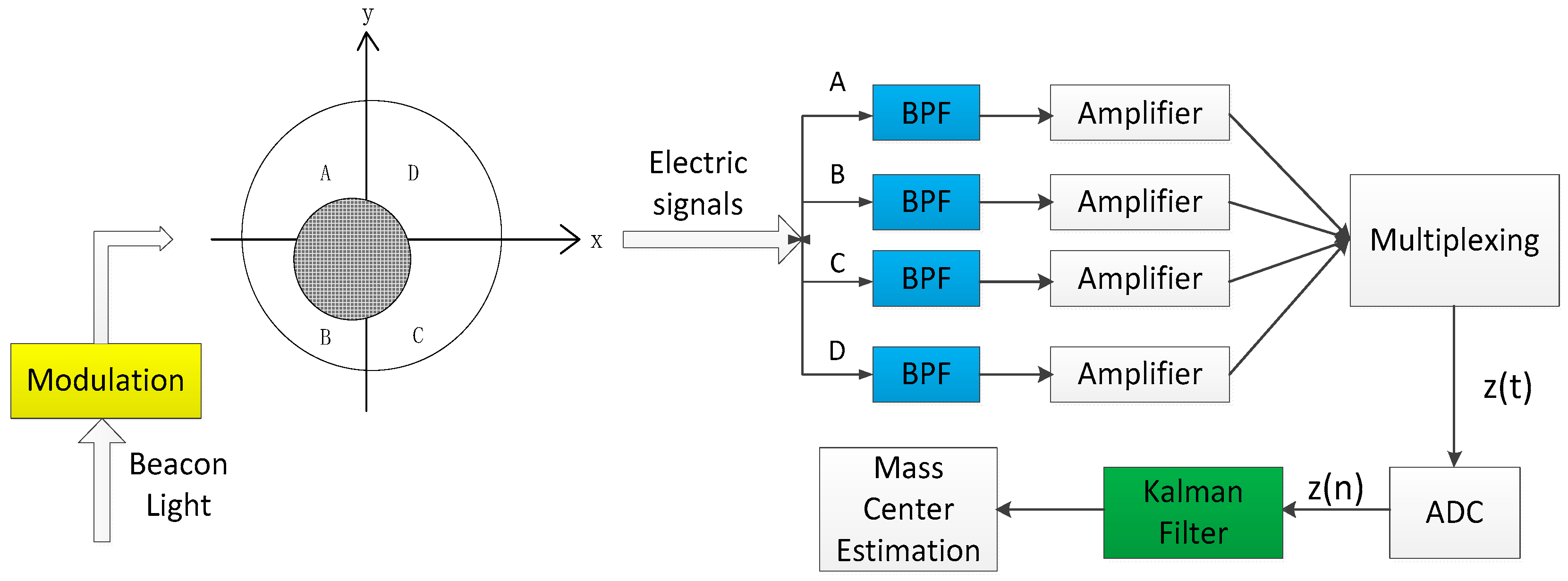
4. Improved Detection Method

The improved detection method can be described as seen in Figure 3.

In Figure 3 we can see, firstly, modulation is added before the beacon light is illustrated on QD. Secondly, low pass filters (LPF) are replaced with band pass filters (BPF) because the modulating signal pulls the frequency spectrum from base frequency to medium frequency. Finally, we use Kalman filtering to eliminate the effect of white noise.

4.1. Modulation of Beacon Light

The direct detection method produces errors because when the electric signals pass through the amplifiers, direct current offsets are brought in. In order to solve this problem, we can adopt the modulation method.

When we apply intensity modulation to the beacon light in the transmitter, we can get the following expressions [13]:

$$E_s\left(t\right)=A\left[1+d\left(t\right)\right]\cos \omega t$$

(5)

$$P_s=\overline{E_s^2\left(t\right)}=\frac{A^2}{2}\left[1+2d\left(t\right)+d^2\left(t\right)\right]$$

(6)

Here, $E_s$ represents the beacon light field, and $P_s$ represents the average power of light field. A is the intensity of beacon light; $d(t)$ is the modulating signal.

After the photoelectric effect and passing through BPF, the photocurrent can be expressed as:

$$I=\frac{e\eta A^2}{hv}d\left(t\right)=Kd\left(t\right)+n\left(t\right)$$

(7)

4.2. Kalman Filtering

Kalman filtering is a time domain method which involves the conception of state space into stochastic estimation theory [14]. It regards the signal transformation as the output of a linear system under the effect of white noise [15]. Using the system state equation, measurement equation, process noise, and measurement noise to describe the input and output makes it become a filtering algorithm [16]. In general, Kalman filtering is used to forecast or filter in the situations we deal with time sequence and white noise or the system, which can be described as the similar model [12].

In Kalman filtering, we consider describing the dynamic system using the following equation [17]:

$$X\left(k+1\right)=\mathsf{\Phi }X\left(k\right)+\mathsf{\Gamma }W\left(k\right)$$

(8)

$$Y\left(k\right)=\mathrm{H}X\left(k\right)+V\left(k\right)$$

(9)

Here, k is the discrete time, and the system state at time k is $X\left(k\right)\in R^n$; $Y\left(k\right)\in R^m$ is the measurement signal of the corresponding state; $W\left(k\right)\in R^r$ is the input white noise; $V\left(k\right)\in R^m$ is the measurement noise. Equation (8) is called state equation and (9) is called the measurement equation. $\mathsf{\Phi }$ is called state transition matrix and $\mathsf{\Gamma }$ is called measurement matrix. The recursion of Kalman filter is described as follows [18].

$$\mathrm{One}\mathrm{step}\mathrm{forecasting}\mathrm{of}\mathrm{state}:\widehat{X}\left(k+1|k\right)=\mathsf{\Phi }\widehat{X}\left(k|k\right)$$

(10)

$$\mathrm{State}\mathrm{updating}:\widehat{X}\left(k+1|k+1\right)=\widehat{X}\left(k+1|k\right)+K\left(k+1\right)\epsilon \left(k+1\right)$$

(11)

$$\mathrm{Filtering}\mathrm{gain}\mathrm{matrix}:K\left(k+1\right)=P\left(k+1|k\right)H^T{\left[HP\left(k+1|k\right)H^T+R\right]}^{-1}$$

(12)

$$\mathrm{One}\mathrm{step}\mathrm{forecasting}\mathrm{of}\mathrm{covariance}\mathrm{matrix}:P\left(k+1|k\right)=\mathsf{\Phi }P\left(k|k\right){\mathsf{\Phi }}^{\mathrm{T}}+\mathsf{\Gamma }Q{\mathsf{\Gamma }}^T$$

(13)

$$\mathrm{Covariance}\mathrm{matrix}\mathrm{updating}:P\left(k+1|k+1\right)=\left[I-K\left(k+1\right)H\right]P\left(k+1|k\right)$$

(14)

$$\widehat{X}\left(0|0\right)={\mu }_0,\widehat{P}\left(0|0\right)=P_0$$

(15)

In one period, Kalman filtering have two information updating processes; these are the time updating process and the measurement updating process. Equation (10) shows the method to estimate and forecast the state of time k using the state of time k − 1; Equation (13) gives a quantified description for the quality being good or bad. Equation (10) and Equation (13) together describe the process of Kalman filtering updating. That is to say, we use the state k − 1 to forecast state k using Equation (10), but the forecasting is not accurate, so we use the variance and some known parameters to estimate the value of the state, which is closer to the real state value. With the increase of k, which means an increase in the iteration steps, the values of state are slowly convergent. All the above steps describe the Kalman filtering method, where we reasonably use measurement value to estimate state value, which is unknown.

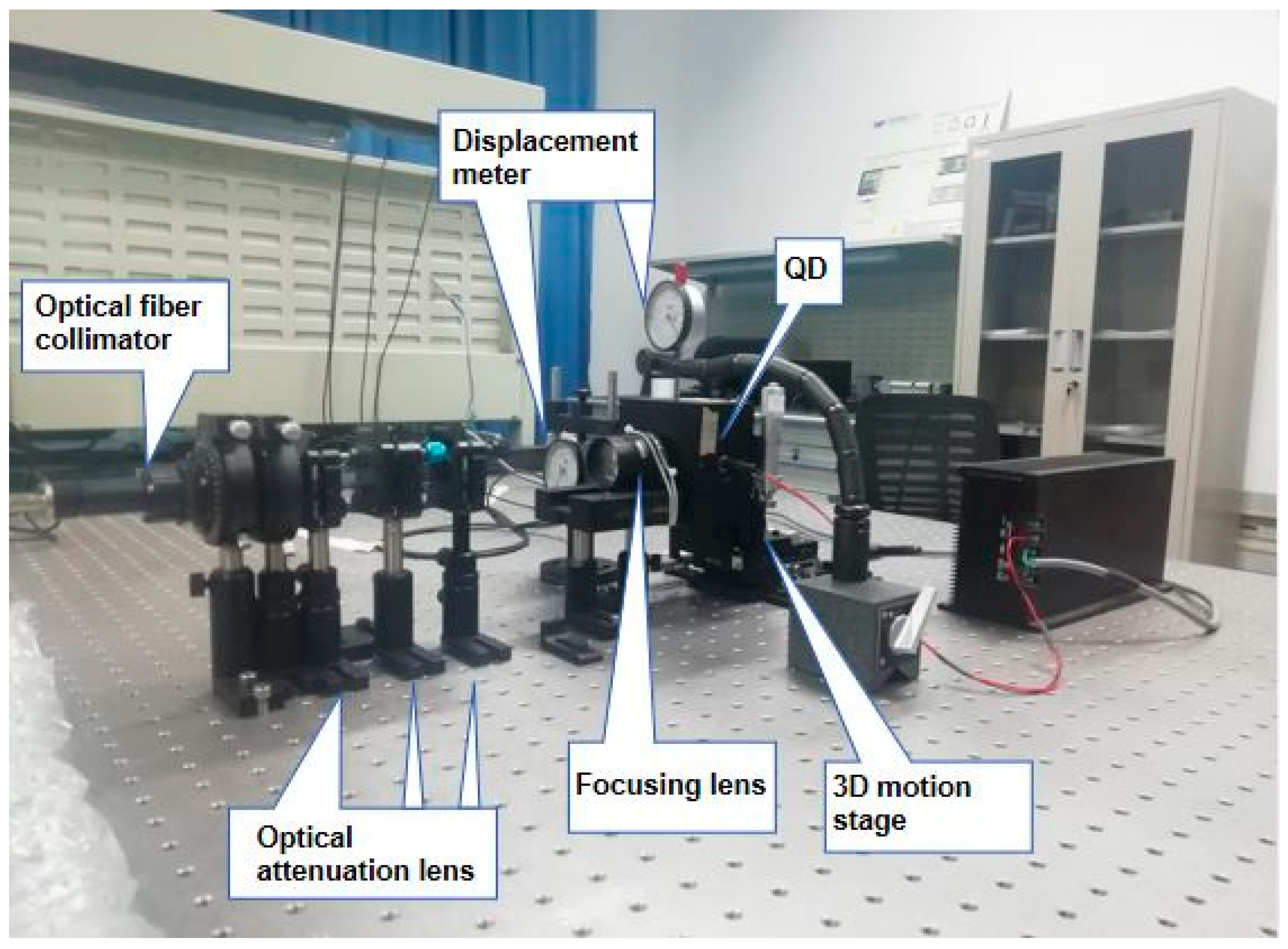
5. Experiment Results

The experiment platform is shown in Figure 4. The laser source we use in the experiment is a modulated laser source with a wavelength of 1550 nm, whose output laser is intensity modulated by a cosine signal of 125 kHz. The data width of the ADC output is 16 bits, and the sampling frequency of the ADC is 100 MHz. The QD, whose active radius of 0.5 mm with a gap width of 0.1 mm, is mounted on a 3-dimensional micro-displacement motion stage in order to get the accurate position of the spot light.

We recorded that the spot radius was 0.42 mm, and the QD output SNR is −10 dB. Here we define that $x_0$ is the calculated x coordinate, and X is the real x coordinate; then we can get the deviation of the spot position (here we regard the coordinate y having the same distribution as x, so we only use the x coordinate for calculation):

$${\delta }_x=x_0-X$$

(16)

There are 800 data points in one period after ADC. Here, we take one period of photocurrent data output from QD using the direct method. For the proposed method, the four electric signals are separately processed in Kalman filters. Before Kalman filtering, we calculate the DC offsets and give an inverse gain to eliminate them.

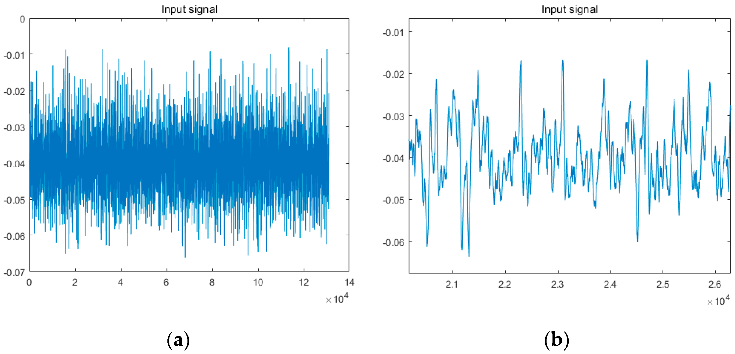
The input modulated signals of one quadrant are shown in Figure 5.

In Figure 5a, the input signal is so dense that in order to see the details, we need to zoom in, as seen in Figure 5b. However, it is also not obvious for us to find out the distribution of the input signals in Figure 5b.

Here, we use the peak values of the signals in every period after ADC as the measurement values. Then we take the peak values of every period, which are directly proportional to the amplitude illustrated on QD, into the iterative formula to estimate the position. The measurement signals contain the real position signals and the noise, where the real position signals should be the same in theory. Therefore, we presume that the variance of the measurement noise is the same as the variance of the measurement signals. In addition, we assume the initial value of the state X(0) is the mean value of the measurement matrix, and then we can calculate the initial covariance P(0). Finally, we use Kalman filtering to estimate the amplitude of the beacon light.

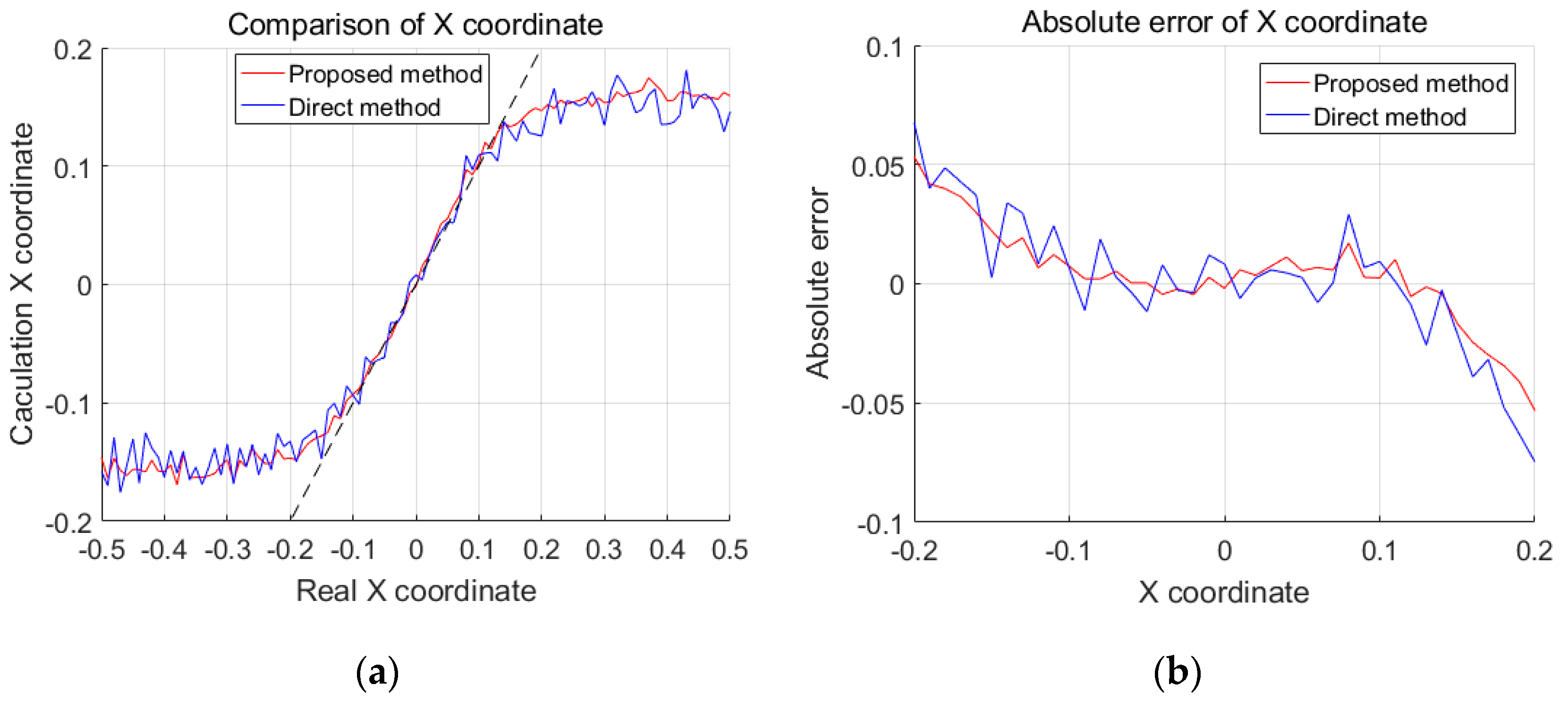
We first take 10 points of peak values into calculation, After the calculation, we can compare the performance of the two processing methods. The experiment results are shown in Figure 6.

In Figure 6a, the black dotted line represents the ideal situations, where the calculated coordinate is the same as the real coordinate. However, there are gaps between the diodes, causing the non-linearity of the QDs between measurement values and real values. The blue solid line represents the direct detection method, and the red solid line represents the proposed improved detection method. The two lines show that the proposed method improves the linearity of QD over the direct method. In Figure 6b, the absolute errors of the proposed method are also smaller than the direct method.

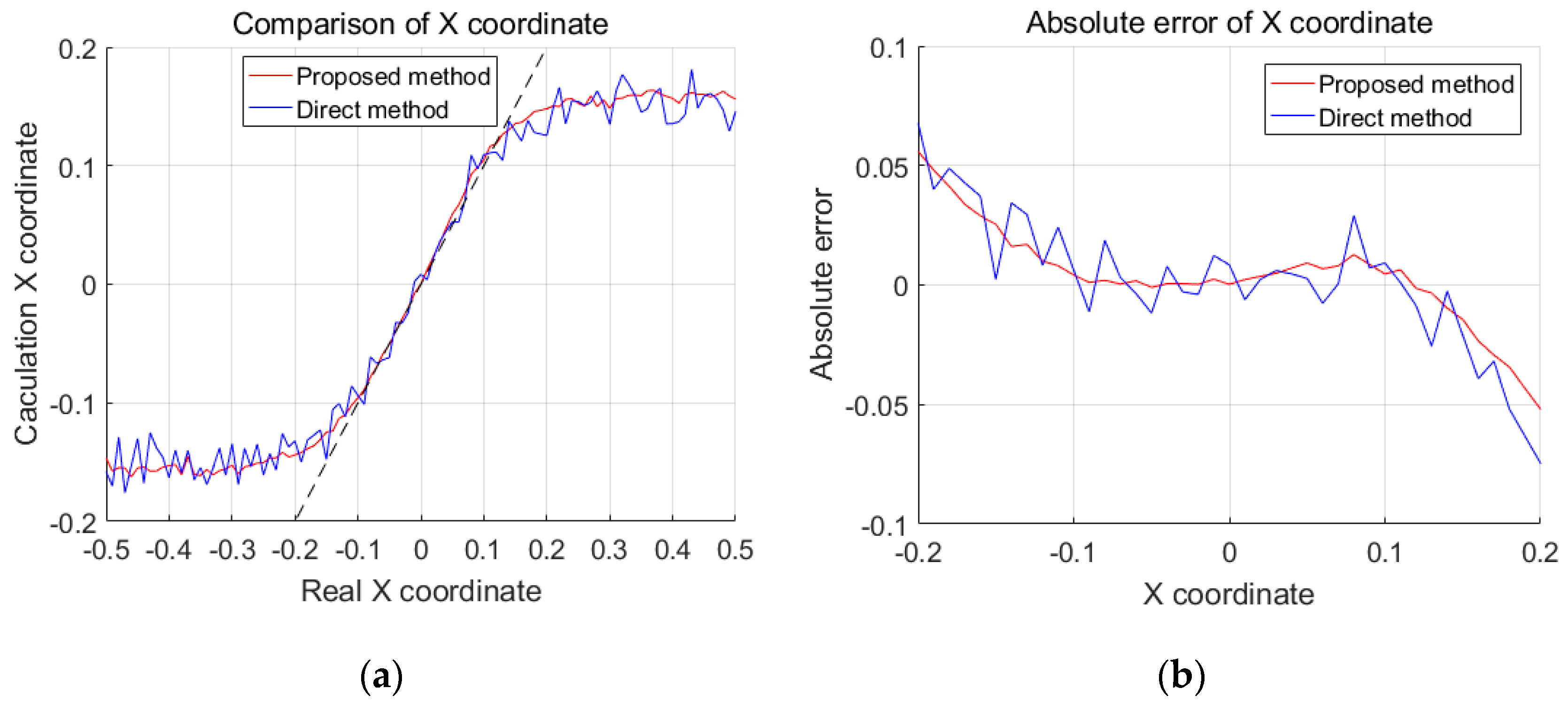
We then add the measurement values up to 40 points, with the experiment results shown in Figure 7.

In Figure 7, we can see that the linearity is almost the same, but the absolute errors decrease compared with Figure 6.

We continue adding the measurement values up to 80 points until the absolute errors do not change, which means the filtering algorithm is already convergent. The experiment results are shown in Figure 8. The decreases in absolute errors are not obvious, so we apply quantified calculation later. Here, we use root-mean-square (RMS) errors to express the result:

$${\delta }_R=\sqrt{{\displaystyle \sum _{i=1}^N{\delta }_i^2/N}}$$

(17)

In Figure 8, the two solid lines show that the method proposed has improved the linearity of QD; it is smoother than the direct detection method. The proposed method can guarantee good linearity within the interval [−0.2, 0.2]. In addition, Figure 8b shows that the absolute errors of the calculated coordinate are smaller using the proposed method rather than the direct method.

Because of the linearity of the QD, if we want to compare the performance of the two methods, we should choose the linearity area. Therefore, we choose the interval [−0.1, 0.1], which is the most linear part, to compare the RMS errors of the two methods. After calculation, the RMS errors are 0.0049 for the proposed method with 80 points Kalman filtering and 0.0101 for the direct method with a period data, which means the RMS error decreases by 51.5%. We list the RMS errors of all the situations in

Table 1. Comparison of the root-mean-square (RMS) errors in different points of iteration.

Points	Proposed Method	Direct Method
10	0.0062 mm	0.0101 mm
40	0.0053 mm
80	0.0049 mm

.

6. Conclusions

In light spot position detection, we use a QD as the detector. However, in the traditional direct detection method, after signals are run through the amplifier, some DC offsets are brought into the QD output electric signals. In order to solve the problem, we considered to use a modulation method and replaced the low pass filters with band pass filters. For white noise, we used a Kalman filter to eliminate it. Then, we made an experimental verification, and the results showed that after using the improved detection method, the linearity of QD was improved and the root-mean-square errors decreased 51.5% compared to the direct detection method. In addition, the QD output SNR was about −10 dB, which means the improved detection method can work in low SNR condition. What is more, Kalman filtering does not require a large amount of data, which means it works efficiently.

References

- Nikulin, V.V.; Khandeka, R.M.; Agile, J.S. Acousto-optic tracking system for free space optical communications. Opt. Eng. 2008, 47, 064301. [Google Scholar] [CrossRef]
- Fan, X.; Zhang, L.; Tong, S.; Song, Y.; Jiang, L. Influence of sky background light on space laser communication system. Laser Optoelectron. Prog. 2017, 54, 102–110. [Google Scholar]
- Fitzsimons, E.D.; Bogenstahl, J.; Hough, J.; Killow, C.J.; Perreur-Lloyd, M.; Robertson, D.I.; Ward, H. Precision absolute positional measurement of laser beams. Appl. Opt. 2013, 52, 2527–2530. [Google Scholar] [CrossRef] [PubMed]
- Wu, J.; Zhao, B.; Wu, Z. Improved measurement accuracy of the spot position on an InGaAs quadrant detector by introducing Boltzmann function. In Proceedings of the International Conference on Optoelectronics and Microelectronics (ICOM), Changchun, China, 16–18 July 2015; pp. 183–185. [Google Scholar]
- Liu, Z.; Steele, J.M.; Lee, H.; Zhang, X. Tuning the focus of a plasmonic lens by the incident angle. Appl. Phys. Lett. 2006, 88, 171108. [Google Scholar] [CrossRef]
- Dang, L.P.; Tang, S.G.; Zhou, Z. Characteristic Analysis and Optimization of Quadrant Detector Output Signal. Opto-Electron. Eng. 2010, 37, 1–6. [Google Scholar]
- Chen, M.; Yang, Y.; Jia, X.; Gao, H. Investigation of positioning algorithm and method for increasing the linear measurement range for four-quadrant detector. Optik 2013, 124, 6806–6809. [Google Scholar] [CrossRef]
- Zhu, Y.; Li, M.; Tang, G.; Jiang, W. Noise analysis of photon counting quadrant detector. Opto-Electron. Eng. 1999, 26, 1–7. [Google Scholar]
- Wang, G. Optical Axis Deviation Detection Technique based on the Balanced Detector. Ms.C. Thesis, Institute of Optics and Electronics, Chinese Academy of Sciences, Beijing, China, 2017. (In Chinese). [Google Scholar]
- Anssi, M. Position-Sensitive Devices and Sensor Systems for Optical Tracking and Displacement Sensing Application. Ph.D. Thesis, Faculty of Technology, University of Oulu, Oulu, Finland, 2000. Available online: http://jultika.oulu.fi/files/isbn9514257804.pdf (accessed on 20 March 2019).
- Shen, C. The Development of Photon Beam Position Monitor System Based on Four-Quadrant Detector; University of Science and Technology of China: Hefei, China, 2009. [Google Scholar]
- Zhao, X.; Tong, S.; Jiang, H. Experimental testing on characteristics of four-quadrant detector. Opt. Precis. Eng. 2010, 18, 2164–2170. [Google Scholar]
- Li, Q.; Xu, S.; Yu, J.; Yan, L.; Huang, Y. An Improved Method for the Position Detection of a Quadrant Detector for Free Space Optical Communication. Sensors 2019, 19, 175. [Google Scholar] [CrossRef]
- Talebi, S.P.; Kanna, S.; Mandic, D.P. A distributed quaternion Kalman filter with applications to smart grid and target tracking. IEEE Trans. Signal Inf. Process. Netw. 2016, 2, 477–488. [Google Scholar] [CrossRef]
- Olfati-Saber, R. Distributed Kalman filtering for sensor networks. In Proceedings of the 46th IEEE Conference on Decision and Control, New Orleans, LA, USA, 12–14 December 2007; pp. 5492–5498. [Google Scholar]
- Qi, W.-J.; Zhang, P.; Nie, G.-H.; Deng, Z.-L. Robust weighted fusion kalman predictors with uncertain noise variances. Digit Signal Process. 2014, 30, 37–54. [Google Scholar] [CrossRef]
- Cattivelli, F.; Sayed, A.H. Diffusion distributed Kalman filtering with adaptive weights. In Proceedings of the Asilomar Conference on Signals, Systems and Computers, Pacific Grove, CA, USA, 1–4 November 2009. [Google Scholar]
- Jiang, T.; Matei, I.; Baras, J.S. A trust based distributed Kalman filtering approach for mode estimation in power systems. In Proceedings of the Workshop on Secure Control Systems, Stockholm, Sweden, 12 April 2010. [Google Scholar]
© 2019 by the authors. Licensee MDPI, Basel, Switzerland. This article is an open access article distributed under the terms and conditions of the Creative Commons Attribution (CC BY) license (http://creativecommons.org/licenses/by/4.0/).