Quantum Classification Algorithm Based on Competitive Learning Neural Network and Entanglement Measure

Abstract

In this paper, we develop a novel classification algorithm that is based on the integration between competitive learning and the computational power of quantum computing. The proposed algorithm classifies an input into one of two binary classes even if the input pattern is incomplete. We use the entanglement measure after applying unitary operators to conduct the competition between neurons in order to find the winning class based on wining-take-all. The novelty of the proposed algorithm is shown in its application to the quantum computer. Our idea is validated via classifying the state of Reactor Coolant Pump of a Risky Nuclear Power Plant and compared with other quantum-based competitive neural networks model.

1. Introduction

Quantum neural networks (QNNs) is a research domain that proposes neural network models based on quantum computing postulates [1]. One of the main advantages of classical artificial neural networks (CANNs) is its ability to perform computations in parallel [2]. However implementing CANNs on traditional computers does not offer this advantage. Traditional computers allow computations based on the bit value that is either “$0$” or “$1$”. R. Feynman suggested that performing that quantum computation is also perfectly possible at the quantum bit (qubit) level [3] on the grounds of the superposition phenomenon. In fact, quantum computations are based on quantum correlations [4,5,6,7], particularly, quantum entanglement [8]. Therefore, the learning phase is expected to be much faster than CANNs due to quantum parallelism.

The birth of QNNs was in 1995 with Kak who tried to link CANNs to quantum mechanics [9]. Consequently, several researchers proposed various models and algorithms of CANNs that attempt to harness the principles of quantum computing and quantum information theory [1]. These algorithms are classified into three main categories. The first category is called QNN’s algorithms [10,11,12,13,14,15,16,17,18,19,20,21]. They are based on quantum mechanics postulates [1] and can be implemented only on quantum computers. The second category is ANNs that are inspired by quantum computing, and exploits some mathematical aspects of quantum information and quantum computation to speed up the learning process of CANNs [22,23,24,25,26,27,28,29,30,31,32,33,34]. However, this kind of ANNs can be implemented only on classical computers rather than physical quantum computers. Finally, the third category of these algorithms is a hybrid model that combines QNNs and CANNs in such a way that some calculations are performed on quantum computers, then based on the outputs of measurement operations, the remaining calculations are performed on classical computers [35,36,37,38].

Competitive learning is one of the unsupervised learning techniques that is inspired by biological brains [2]. This type of learning allows for competition among neurons, and ends with a single winner neuron. The winning neuron has the most similar pattern to an input test pattern. Because this competition allows only one neuron to be a winner, it is called winner-take-all competition. This competition is often used in Hamming neural networks [2,39] which is used to solve some classification problems intractable for other CANNs. There are four models proposed to implement quantum competitive learning, two of these models are not applicable on physical quantum systems [23,38], while the other two models have unreliable results [21,40]. To overcome the defects of the previous models, we exploit the power of quantum computing to propose a novel quantum classifier by harnessing both the superposition and entanglement to implement competitive learning on quantum systems. In this paper, we propose a novel quantum classification model that exploits the superposition property to allow the competition between the neurons by applying the CNOT-gate, between the register of the input pattern and the register that stores prototypes patterns, and applying the quantum NOT-gate on the register that stores prototypes patterns. Then the Toffli-gate is used to mark the wining neuron that represents that class. This winning neuron could have zero value state, $|0\rangle$, or one value state, $|1\rangle$. So, in order to find the value of the wining neuron, we need to implement the winner-take-all technique. To implement this technique, we propose to use one of the entanglement measures called concurrence, so that if the wining neuron has zero value state $|0\rangle$, then the corresponding value of concurrence is zero. Conversely, if the wining neuron has one value state $|1\rangle$, then the value of concurrence is one. Due to the proposed classification model harnesses the superposition property of quantum mechanics, it outperforms the classical model in two ways. First, it performs the competition between neurons exponentially faster than classical competitive neural networks. Second, the proposed model uses Zhou’s storage model [20] to store the prototypes patterns, therefore the storage capacity is increased exponentially compared to classical models. The proposed model also recognizes the wining class by quantifying the concurrence value that is more accurate than Zhou’s quantum model [21] that recalls the state of the wining pattern with probability $\frac{1}{M}$, where M is the number of the prototypes patterns. The efficiency of the proposed model is verified by using the dataset of Risky Nuclear Power Plant to identify the state of the Reactor Coolant Pump (RCP), and to classify it into one of two classes, low-risk (labeled as class “0”) or high-risk (labeled as class “1”). Then, the classification accuracy of the proposed model is compared with the classification accuracy of Zhou’s model [21].

This paper is organized as follows: Section 2 reviews the related work of quantum competitive learning. In Section 3, we briefly review some basic quantum concepts and the quantum gates that will be used to propose the quantum competitive model. In Section 4, we demonstrate the methodology used to apply winner-take-all using quantum aspects. Section 5 explains the proposed algorithm and shows how can be applied on a case study. Section 6 discusses the experimental results and shows the effectiveness of the proposed algorithm to classify a real-world dataset based on the principle of competitive learning. Finally, Section 7 concludes the paper and presents some possible research perspectives.

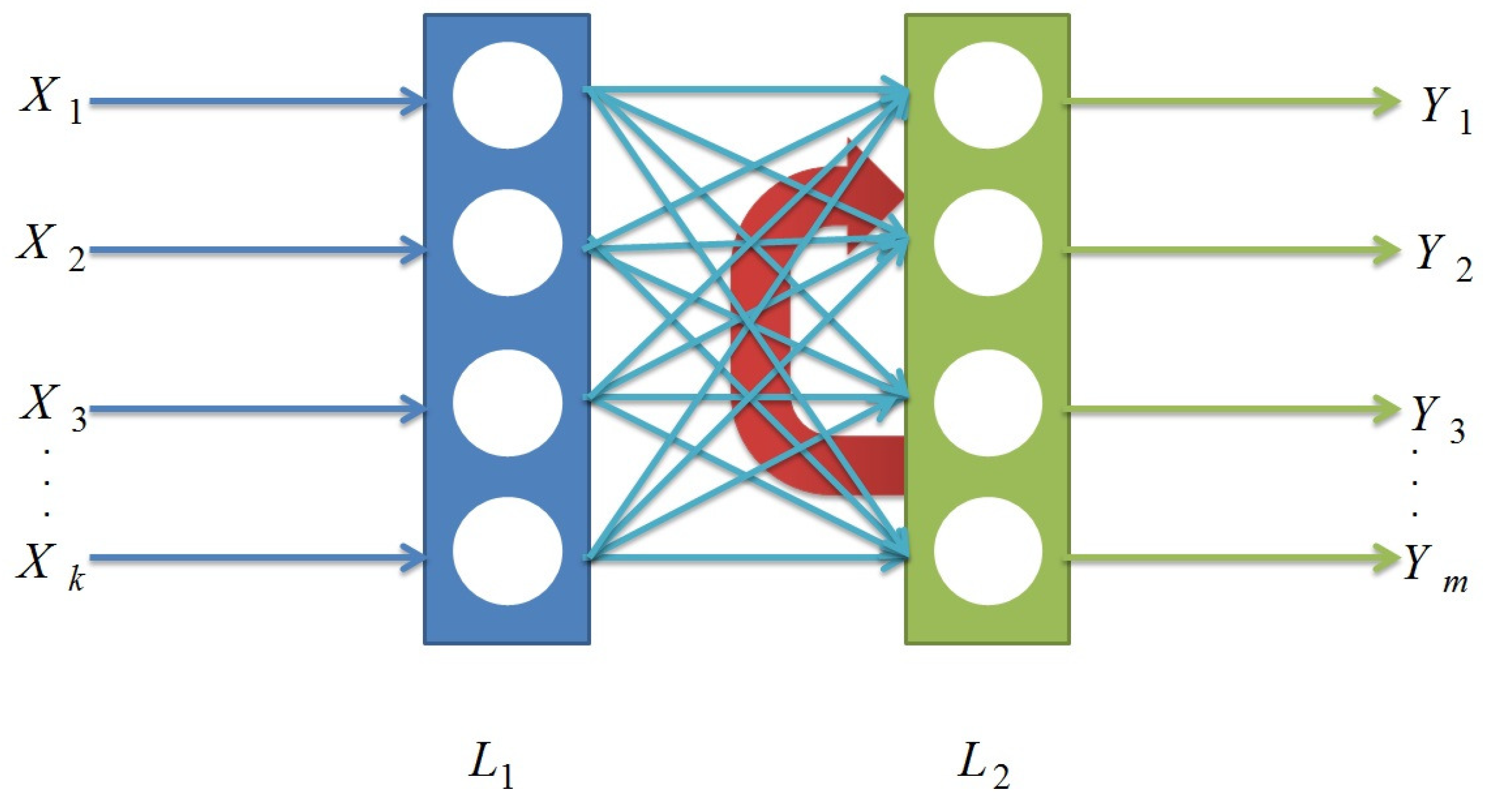
2. Quantum Competitive Learning

A well-known learning technique in ANNs is competitive learning. The technique is useful for classification applications and has the potential to implement associative memory for a set of predefined patterns. Competitive learning is inspired in biological neural networks, and accommodates ANNs based on a neural configurations where only one neuron fires, winner-take-all, at a tine at a given iteration. In competitive learning, a neuron will be a winner if it has the largest weighted input compared with the other neurons in the competitive layer. Several neural network algorithms based on the competitive learning were proposed such as the Hamming neural network (HNN), self-organizing feature map (SOM) and learning vector quantization (LVQ) [2].

HNN is used to find the degree of similarity between an input vector and the weight vector of each neuron in the network. HNN consists of two layers L1 and L2. L1 is called the input matching layer, while L2 is called the competitive layer. The Hamming distance between an input pattern and prototype patterns is calculated via Layer, whereas the most matched storage pattern to the input pattern is obtained based on the rule of minimum distance, via L2 layer. Figure 1 shows the topology structure of the classical HNN.

Four models of competitive learning based on quantum properties have been proposed to maximize the efficiency of classical competitive neural networks. The first model was developed in 1999 by Ventura [23], who proposed a competitive learning algorithm inspired by the properties of quantum computing to be implemented on traditional computers only. Moreover, the learning algorithm of this model requires to be adapted with threshold parameter depending on the application at hand. The second model, developed by Zhou [20,21] in 2007, established the quantum algorithm that stores a set of predefined patterns in the memory of n neurons. This model increases the storage capacity of the neurons exponentially in contrast to classical neurons. Then, in 2010, Zhou proposed a quantum version of competitive CANNs that comprised two phases. The first phase is the storing phase, and is used to store the patterns in the neurons of the competitive ANNs. In the second phase, the competitive phase, Zhou proposed a quantum algorithm that allows the competition between neurons when an input pattern is presented to the network [21]. The primary defect of Zhou’s competitive model [21] that the wining pattern is decided with low probability, because this model recalls the wining pattern based on decreased probability of the undesired patterns. Therefore, the probability of the wining pattern is decreased as the number of the stored patterns increases in the storing phase [38]. Zhong and Yuan proposed the third model of quantum competitive learning using Grover’s algorithm [41]. This is in order to perform the competition between the neurons to recall the wining pattern when an incomplete pattern is presented to their model [40]. They showed that recalling pseudo-patterns is inevitable on their competitive model [40]. The final model was developed in 2015 is called HQNN model [38]. In this model, competitive learning is conducted as a hybrid of quantum and classical computation so that the competitive phase is performed on two competitive layers. The first layer allows competitions between neurons using quantum gates, where the second layer uses nonlinear operation to find the winning neuron based on the winner-take-all technique. Unlike the Ventura model [23], HQNN model [38] does not have a threshold parameter, and unlike Zhou’s model [21], it recalls the winning pattern only and discards the undesired patterns. Additionally, HQNN model does not recall pseudo patterns as Zhong’s and Yuan’s model does [38], however, it cannot be fully implemented in real quantum computers because the winning pattern is only retrievable using classical operation.

3. Qubits and Quantum Gates

3.1. Qubit

The fundamental element in quantum computer is called quantum bit (qubit). It stores information based on the superposition phenomena [1] of “0” and “1”, in the form

$$|\varphi \rangle =\mu |0\rangle +\lambda |1\rangle ,$$

the coefficients $\mu$,$\lambda$ are complex numbers where ${\left|\mu \right|}^2+{\left|\lambda \right|}^2=1$. After the measurement process, the state of the qubit $|\varphi \rangle$ collapses into a state $|0\rangle$ or a state $|1\rangle$ with probability ${\left|\mu \right|}^2$ or ${\left|\lambda \right|}^2$, respectively.

3.2. Quantum Gates

According to quantum mechanics postulates [1], the evolution of the quantum systems is allowed only through unitary operators. An arbitrary operator A is unitary if and only if AA${}^{†}=A^{†}A=I$, where $A^{†}={(A^{*})}^T$. So, quantum gates are unitary operators. So far, quantum computations are performed practically through the quantum circuit model. The proposed competitive algorithm uses quantum negation gate X, CNOT gate and finally the Toffoli-gate. The quantum negation gate, $X=|1\rangle \langle 0|+|0\rangle \langle 1|$, negates the state of a qubit. CNOT gate, $CNOT|u,v\rangle =|u,(u+v)mod2\rangle$, is acting on two qubits together one of them is the control qubit, and the other is the target qubit. This gate negates the state of the target qubit only if the state of the control qubit is “$1$”. On the other hand, Toffoli gate ($T^2$) acts up on three qubits, two of which are used as control qubits, and the third is the target qubit. The whole gate is described as follows [42]:

$$T^2|uvw>=|uv,(w+(u.v))mod2\rangle ,$$

In other words, Toffoli gate ($T^2$) negates the third qubit only if the first two qubits are in the state $|11\rangle$. The general form of applying the Toffoli gate ($T^j$) on $j+1$ qubits is defined as:

$$T^j|u_1{u}_2\dots u_j{u}_{j+1}>=|u_1{u}_2\dots u_j,(u_{j+1}+\prod _{p=1}^j{u}_p)mod2\rangle ,$$

(1)

where the superscript j represents the number of control qubits. Toffoli ($T^j$) gate negates the indexed qubit $u_{j+1}$ only if the first j qubits are in the state $|11\dots 1\rangle$. These gates will be used to propose the quantum classification algorithm based on competitive neural network (see Section 5).

4. Methodology

Entanglement is a type of the quantum correlations [6,43,44,45,46,47,48] that distinguishes the behavior of quantum mechanics. A two-qubit system becomes an entangled states if the state of one qubit cannot be separated from the state of the other. Entanglement cannot be detected directly, so entanglement measures [49,50,51] were proposed to determine the degree of entanglement in a quantum system. Various measurements are proposed to measure the strength of the entanglement between two-qubit systems such as concurrence, witness, and negativity among others [50,52,53]. However, the strength of entanglement in a two-qubit system is often measured using concurrence measure [50,51]. An arbitrary, pure two-qubit state has the form

$$|\psi \rangle =\alpha |00\rangle +\beta |01\rangle +\gamma |10\rangle +\delta |11\rangle ,$$

(2)

its concurrence measure is defined theoretically as follows [54]:

$$C=2|\alpha \delta -\gamma \beta |,$$

(3)

where $0\le C\le 1$. It is obvious that if the state of the two-qubit system is defined by the state $\alpha |00\rangle +\beta |11\rangle$, the concurrence value becomes $2|\alpha \beta |$[55]. Concurrence measure operator, denoted $M_z$, was proposed to solve some quantum computation problems [56]. For example, some researchers used this operator to increase the computational speed for testing junta variables [57] and measuring the Hamming distance between boolean functions [58] quantum mechanically. The circuit model of $M_z$ operator was proposed as shown in Figure 2 when applied on arbitrary two qubits $|u\rangle$ and $|v\rangle$. The state of the qubit $|v\rangle$ is initialized in the vacuum state $|0\rangle$ and the state of the qubit $|u\rangle$ is arbitrary. The $M_z$ is a unitary operator that applies the $CNOT$ gate between the qubits $|u\rangle$ and $|v\rangle$ followed by measuring the degree of entanglement in between through the operator D. The $M_z$ operator creates the entangled state $|uv\rangle =\alpha |00\rangle +\delta |11\rangle$, then it measures the concurrence between the qubits $|u\rangle$ and $|v\rangle$ as $C>0$ through the operator D only if the input qubit $|u\rangle$ is in the state $|u\rangle =\alpha |0\rangle +\delta |1\rangle$, while it leaves them disentangled in the state $|uv\rangle =|00\rangle$, then it measures the concurrence value in between as $C=0$ through the operator D only if the input qubit $|u\rangle$ is in the state $|u\rangle =|0\rangle$.

Some suggestions to implement the operator D using experimental setups are depicted in [51,55,59]. However, concretely in this paper, we propose to implement the operator D in the operator $M_z$ using Romero et al. protocol [54]. This protocol implements Equation (3) quantum mechanically, and the circuit model of this protocol is depicted in Figure 3. This protocol requires two copies of the two-qubit pure state given by Equation (2). This protocol is summarized in the following steps:

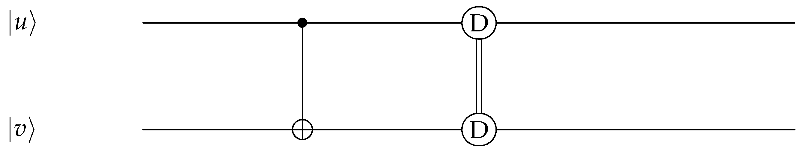
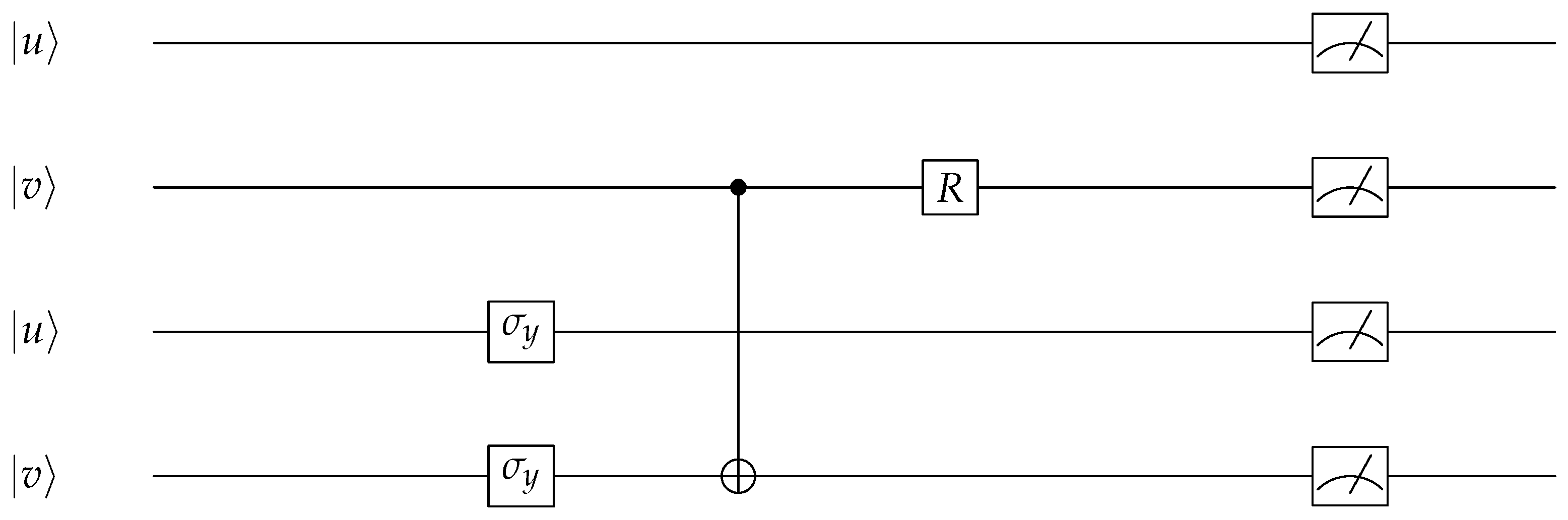
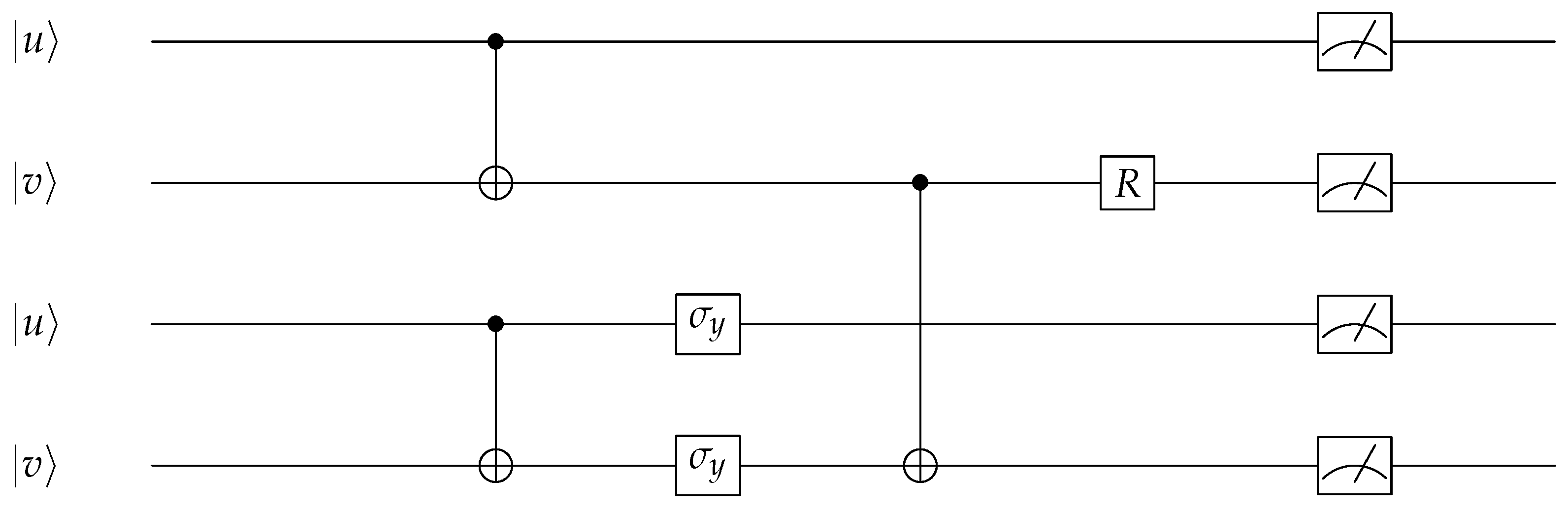
• Prepare two copies of the two-qubit state given by Equation (2) as follows:

  $$|{\eta }_0\rangle =|\psi \rangle ({\sigma }_y\otimes {\sigma }_y|\psi \rangle ).$$
• $CNOT$ gate is applied between the second and the forth qubits, respectively, followed by the rotation R gate as follows:

  $$|{\eta }_1\rangle =RCNO{T}_{{\eta }_{0_2}{\eta }_{0_4}}|{\eta }_0\rangle ,$$

  where the subscripts in the $CNO{T}_{{\eta }_{0_2}{\eta }_{0_4}}$ gate represent the control and the target gate, respectively. However, the unitary R gate rotate the state of the qubit as follows:

  $$R|0\rangle =\frac{|0\rangle -|1\rangle }{\sqrt{2}},R|1\rangle =\frac{|0\rangle +|1\rangle }{\sqrt{2}}.$$

  Therefore, the state of the system is as follows:

  $$\begin{array}{ccc}\hfill |{\eta }_1\rangle =\frac{1}{\sqrt{2}}& \{& (\beta \gamma -\alpha \delta )|0000\rangle +(\beta \gamma +\alpha \delta )|0100\rangle +(\alpha \gamma -\beta \delta )|0001\rangle -(\alpha \gamma +\beta \delta )|0101\rangle +2\gamma \delta |1100\rangle \hfill \\ & & -2\alpha \beta |0110\rangle +({\beta }^2-{\alpha }^2)|0011\rangle +({\beta }^2+{\alpha }^2)|0111\rangle +({\gamma }^2-{\delta }^2)|1001\rangle -({\gamma }^2+{\delta }^2)|1101\rangle \hfill \\ & & +(\beta \gamma -\alpha \delta )|1010\rangle -(\beta \gamma +\alpha \delta )|1110\rangle +(\alpha \gamma +\beta \delta )|1111\rangle -(\alpha \gamma -\beta \delta )|1011\rangle \}.\hfill \end{array}$$

  (4)

  Comparing Equation (3) and Equation (4), we obtain

  $$C=2\sqrt{2P_{0000}}orC=2\sqrt{2P_{1010}},$$

  (5)

  where $P_{0000}$ and $P_{1010}$ are the success probability for obtaining the state $|0000\rangle$ and $|1010\rangle$, respectively.

end.

So, taking this into account, our proposal to implement the operator D using Romero et al. circuit [54], transforms the circuit model of the $M_z$ operator from Figure 2, Figure 3 and Figure 4. It is obvious that $M_z$ operator applies two main operations. In the first operation, the $CNOT$ gate is applied on each replica of the two-qubit systems $|u\rangle$ and $|v\rangle$ as the control qubit and as a target qubit, respectively. Accordingly, there are two cases:

(i) The state of each replica of the two-qubit $|uv\rangle$ system will be entangled, $|uv\rangle =\alpha |00\rangle +\delta |11\rangle$, only if $|u\rangle =\alpha |0\rangle +\delta |1\rangle$. Consequently, when the second operation of the operator $M_z$ operator is applying the operator D on the state $|uv\rangle \otimes |uv\rangle$ as shown in Figure 4. Therefore, the state of the system is as follows:

$$|{\eta }_1\rangle =\frac{1}{\sqrt{2}}\{-\alpha \delta |0000\rangle +\alpha \delta |0100\rangle -{\alpha }^2|0011\rangle -\alpha \delta |1010\rangle +{\alpha }^2|0111\rangle -{\delta }^2|1001\rangle -{\delta }^2|1101\rangle -\alpha \delta |1110\rangle \}.$$

(6)

Comparing Equation (3) and Equation (6), we obtain

$$C=2\sqrt{2P_{0000}},C=2\sqrt{2P_{0100}},C=2\sqrt{2P_{1010}}orC=2\sqrt{2P_{1110}}.$$

(7)

Then the concurrence can be estimated using one of the formulas shown in Equation (7).

(ii) On the other hand, the state of the system will be separable in the state $|uv\rangle =|00\rangle$ if the state of the qubit $|u\rangle$ is $|0\rangle$. Again, when the second operation of the operator $M_z$ operator is applying the operator D on the state $|uv\rangle \otimes |uv\rangle$ as shown in Figure 4. Therefore, the state of the system is as follows:

$$|{\eta }_1\rangle =\frac{1}{\sqrt{2}}\{-{\alpha }^2|0011\rangle +{\alpha }^2|0111\rangle \}.$$

(8)

So, in this case the concurrence value is $C=0$. Eventually, the operator D in $M_z$ operator measures the concurrence value between the two qubits $|u\rangle$ and $|v\rangle$, by estimating the probability of obtaining the probability of the state $|0000\rangle$, $|0100\rangle$, |$1010\rangle$, or $|1110\rangle$, therefore the concurrence value is given by Equation (7). $M_z$ will be used in the last step int the proposed algorithm (see Section 5).

5. The proposed Quantum Classification Algorithm Based on Competitive Learning and Entanglement Measure: Case Study

Quantum competitive neural networks consists of two layers namely quantum-storing layer and quantum-competitive layer [21,38]. Quantum-storing layer stores M defined prototype patterns in advance with equal probabilities via n neurons using the Zhou’s storage model (for more details see Section 5.1). Here, we propose the quantum classification algorithm based on competitive neural network. As for the quantum-competitive layer, the QCPNN algorithm classifies the input pattern into one of two classes “$0$” or “$1$”. In this layer, the steps of the QCPNN algorithm conduct a competition between the prototype patterns to mark, by entanglement, the class of the closest prototype pattern to the input pattern. Eventually, to determine the winning class based on winner-take-all property, $M_z$ operator output only the winning class based on the value of the concurrence. The steps of the QCPNN algorithm are shown in Algorithm 1. According to step 1, the quantum system is initialized by three quantum registers, arranged as $|inp,qn,uv\rangle$. In step 2, when an input pattern is presented to QCPNN algorithm via register $|inp\rangle$, the competition process is performed by detecting the overlapping qubits between the register $|inp\rangle$ and the register $|qn\rangle$, by applying the $CNOT$ gate followed by the negation quantum gate X. Hence, the winning class, which is entangled with the matched pattern, is marked by entanglement via applying the Toffoli-gate $T^{j+1}$ in step 3. This gate flips the state of the qubit $|u\rangle$ to state $|1\rangle$ if the winning class is “1”, therefore, the state of the qubit $|u\rangle =\sqrt{\frac{M-1}{M}}|0\rangle +\sqrt{\frac{1}{M}}|1\rangle$. On the other hand, the gate $T^{j+1}$ leaves the state of the qubit $|u\rangle$ with no effect if the winning class is “0”, therefore, the state of the qubit $|u\rangle =|0\rangle$.

Algorithm 1 The proposed Quantum Classification Algorithm based on Competitive Learning and Entanglement Measure (QCPNN).

For an input pattern $inp$ do{ 1. Initialization Step: $|{\psi }_0\rangle =|inp,qn,uv\rangle .$ Here, the quantum system is initialized by three quantum registers $|inp\rangle$, $|qn\rangle$ and $|uv\rangle$ of size n, $n+1$ and 2 qubits, respectively. The register $|qn\rangle$ represents the memory register that holds the prototype patterns, while $|u\rangle$ and $|v\rangle$ are the states of the other qubits. The first n qubits of the register $|qn\rangle$ store the M prototype patterns, and the last qubit stores the class of the associated pattern. The input pattern that has a set h of j elements, where (j≤n) is presented to the network via the register $|inp\rangle$. The set h contains the indices of the qubits that have well known values. Finally, $|uv\rangle$ is a two-qubit control register which are initialized by state $|00\rangle$. 2. Apply the competitive detection operator between the input register $|inp\rangle$ and the prototype register $|qn\rangle$ as follows: $$|{\psi }_1\rangle =\prod _{i\in h}{X}_{q{n}_i}CNO{T}_{in{p}_{i}q{n}_i}|{\psi }_0\rangle .$$ In this step, the $CNOT$ gate is applied between each qubit $i\in h$, of the resiter $inp$ as a control qubit and the corresponding qubit i in the register $qn$ as a target qubit. Then the negation gate X is applied on each qubit $i\in h$ in the register $qn$. 3. Apply the Toffoli gate between $j+1$ qubits of the register $|qn\rangle$ as control qubits and the qubit $|u\rangle$ as target qubit as follows: $$|{\psi }_2\rangle =T_{({\prod }_{i\in h}q{n}_{i}q{n}_{n+1}u)}^{j+1}|{\psi }_1\rangle .$$ In this step, the Toffoli gate ($T^{j+1}$) is applied on $j+2$ qubits, where the superscript $j+1$ represents the number of control qubits. Toffoli gate ($T^{j+1}$) negates the qubit u if the state of each qubit i belongs to the h and the state of the qubit $q{n}_{n+1}$ are in the state $|1\rangle$. 4. Repeat the steps 1, 2 and 3 to get another copy of $|uv\rangle$ because $M_z$ operator needs two copies to quantify the degree of concurrence in between (see Section 4). Remark: this step does not violate the non-cloning theorem [60] because when steps 1, 2 and 3 are repeated, a new different system is initialized in the first step and when the second and third steps are applied then a new copy of $|uv\rangle$ is created, independently, without cloning the original state. 5. Apply the operator $M_z$, shown in Figure 4, on the two copies of the state $|uv\rangle$ and quantify the probability of the state $|0000\rangle$, $|0100\rangle$, $|1010\rangle$ or $|1110\rangle$ and use Equation (7) to quantify the concurrence value C.    if $C=0$ then    inp ∈ class label "0".    Else if  $C>0$  then    inp $\in 1$ class label "1". } End.

In step 4, steps 1, 2 and 3 are repeated to generate a duplicate of the two-qubit system $|uv\rangle$ that does not violate the non-cloning theorem [60], because $M_z$ operator requires two copies to quantify the degree of concurrence between the qubits $|u\rangle$ and $|v\rangle$ as explained in Section 4. Finally, in step 5, the $M_z$ operator is applied on the two copies of $|uv\rangle$ to test the presence of entanglement between $|u\rangle$ and $|v\rangle$ by estimating the probability of the state $|0000\rangle$, $|0100\rangle$, $|1010\rangle$ or $|1110\rangle$ and use Equation (7) to quantify the concurrence value C. If the concurrence is $C=0$, then the winning class is “0”. On the other hand, if the value of the concurrence is $C>0$, then the label of the winning class is “1”.

5.1. Case Study

To explain the proposed algorithm in more detail, we will explain the proposed algorithm on the following synthesis data set. Suppose that we have a data set from two classes that are labeled “0” and “1”. The prototype patterns of the class that is labelled by class “1” are three patterns in four attributes given as 1110, 1100 and 1011, while the prototype patterns of the class label “0”, also, are three patterns in four attributes given as 0100, 0010 and 0001. So, the set of the prototype patterns can be written as follows:

$$Pt=\left\{11101,11001,10111,01000,00100,00010\right\},$$

(9)

where in each pattern in the set Pt the first four values represent the attributes of the pattern, while the last value represents the class label. Assume that we have an incomplete input pattern that has missing attributes, e.g. $inp=1?0?$, the sign “?” means that this pattern is incomplete in the second and the fourth qubits. To store M, where $M=6$, predefined prototype patterns which are given by Equation (9) with equal probabilities in the quantum-storing layer, we use Zhou’s storage model.

5.1.1. Quantum-Storing Layer Using Zhou’s Storage Model

Zhou’s storage model is initialized by three disentangled registers as follows: $|p\rangle$, $|qn\rangle$, and $|c\rangle$, the first and the second registers are composed of n qubit, while the third register is called the quantum control register that is a two-qubit system is initialized with the state $|01\rangle$. The register $|p\rangle$ is called the input register that stores the the classical prototype pattern $p\in Pt$ into the quantum register $|qn\rangle$. Now lets processed to summarize the “quantum-sorting” in the following eight steps [20,38]:

• Step 1: The quantum system is initialized by the three registers $|p\rangle$, $|qn\rangle$ and $|c\rangle$ as $|{\psi }_0\rangle$= $|p,qn,c\rangle$. Assuming that the input state is given by $p=11101$, where the first pattern in Equation (9) is considered, so the initial state can be described as $|{\psi }_0\rangle$= $|11101,00000,01\rangle$.
• Step 2: $|{\psi }_1\rangle$ = ${\prod }_{i=1}^{n=5}{T}_{p_i{c}_{2}q{n}_i}^2|{\psi }_0\rangle =|11101,11101,01\rangle ,$ where $T^2$ is the toffli gate (Equation (1)).
• Step 3: $|{\psi }_2\rangle$ = ${\prod }_{i=1}^{n=5}NO{T}_{q{n}_i}XO{R}_{p_{i}q{n}_i}|{\psi }_1\rangle =|11101,11111,01\rangle .$
• Step 4: $|{\psi }_3\rangle$ = $T_{q{n}_{1}q{n}_{2}q{n}_{3}q{n}_{4}q{n}_5{c}_1}^{n=5}|{\psi }_2\rangle =|11101,11111,11\rangle .$
• Step 5: $|{\psi }_4\rangle$ = $S_{c_1{c}_2}^6|{\psi }_3\rangle =\frac{1}{\sqrt{6}}|11101,11111,10\rangle +\sqrt{\frac{5}{6}}|11101,11111,11\rangle$, where S is a Venture and Martinez’s gate operator [10,20] that is defined as follows:

  $$S^J=\left[\begin{array}{cccc}1& 0& 0& 0\\ 0& 1& 0& 0\\ 0& 0& \sqrt{\frac{J-1}{J}}& \frac{1}{\sqrt{J}}\\ 0& 0& \frac{-1}{\sqrt{J}}& \sqrt{\frac{J-1}{J}}\end{array}\right]$$

  (10)

  where J is the index of the pattern in the patterns set $pt$.
• Step 6: $|{\psi }_5\rangle$ = $T_{q{n}_{1}q{n}_{2}q{n}_{3}q{n}_{4}q{n}_5{c}_1}^{n=5}|{\psi }_4\rangle =\frac{1}{\sqrt{6}}|11101,11111,00\rangle +\sqrt{\frac{5}{6}}|11101,11111,01\rangle .$
• Step 7: $|{\psi }_6\rangle$ = ${\prod }_{i=1}^{n=5}XO{R}_{p_{i}q{n}_i}NO{T}_{q{n}_i}|{\psi }_7=\frac{1}{\sqrt{6}}|11101,11101,00\rangle +\sqrt{\frac{5}{6}}|11101,11101,01\rangle .$
• Step 8: $|{\psi }_7\rangle$ = ${\prod }_{i=1}^{n=5}{T}_{p_i{c}_{2}q{n}_i}^2|{\psi }_6\rangle =\frac{1}{\sqrt{6}}|11101,11101,00\rangle +\sqrt{\frac{5}{6}}|11101,00000,01\rangle .$

So, it is clear that the pattern $|11101\rangle$ is stored in the first term of the quantum system ($|{\psi }_7\rangle$). Since, the value of $|c\rangle$ register is $|01\rangle$ in the second term of the quantum system $|{\psi }_7\rangle$, consequently the second pattern $|11001\rangle$ will be stored in the second term of the quantum system $|{\psi }_7\rangle$ when the quantum-storing algorithm is repeated again. The same procedure will be performed for the remaining prototype patterns. At the end of this storing phase, we will find both of the registers $|p\rangle$ and $|c\rangle$ are separable with the register memory $|qn\rangle$. That means the output of the quantum-storing layer using Zhou’s storage model is the register $|qn\rangle$ that stores the prototype patterns of the set $Pt$ in a uniform superposition as follows:

$$|qn\rangle =\frac{1}{\sqrt{6}}(|11101\rangle +|11001\rangle +|10111\rangle +|01000\rangle +|00100\rangle +|00010\rangle ).$$

(11)

5.1.2. Classification an Input Using the Proposed Algorithm

Here, we processed to classify the incomplete pattern $inp=1?0?$ using the proposed algorithm in Section 5 according to the following steps

• Initialization Step: $|{\psi }_0\rangle =|inp,qn,uv\rangle .$
  Here, the input register is $|inp\rangle =|1?0?\rangle$, $|qn\rangle$ is the memory register that holds the prototypes patterns and its state is given by Equation (11), and $|uv\rangle$ is initialized by the state $|00\rangle$. Due to the input, test, pattern $|inp\rangle =|1?0?\rangle$ has two well known values in the first and third qubits, so $h=\{1,3\}$. Therefore, the state of the system is described as follows:
  $|{\psi }_0\rangle =\frac{1}{\sqrt{6}}(|1?0?,11101,00\rangle +|1?0?,11001,00\rangle +|1?0?,10111,00\rangle +|1?0?,01000,00\rangle +|1?0?,00100,00\rangle +|1?0?,00010,00\rangle ).$
• Apply the competitive detection operator between the input register $|inp\rangle$ and the prototype register $|qn\rangle$ as $|{\psi }_1\rangle ={\prod }_{i\in h=\{1,3\}}{X}_{q{n}_i}CNO{T}_{in{p}_{i}q{n}_i}|{\psi }_0\rangle$.
  $|{\psi }_1\rangle =\frac{1}{\sqrt{6}}(|1?0?,11001,00\rangle +|1?0?,11101,00\rangle +|1?0?,10011,00\rangle +|1?0?,01100,00\rangle +|1?0?,00000,00\rangle +|1?0?,00110,00\rangle ).$
• Apply the Toffoli-gate between $j+1$ qubits of the register $|qn\rangle$ and the qubit $|u\rangle$ as control qubits and target qubit, respectively.

  $$|{\psi }_2\rangle =T_{({\prod }_{i\in h=\{1,3\}}q{n}_{i}q{n}_{n+1}u)}^{j+1}|{\psi }_1\rangle =T_{(q{n}_{1}q{n}_{3}q{n}_{5}u)}^3|{\psi }_1\rangle .$$
  $|{\psi }_2\rangle =\frac{1}{\sqrt{6}}(|1?0?,11001,00\rangle +|1?0?,11101,10\rangle +|1?0?,10011,00\rangle +|1?0?,01100,00\rangle +|1?0?,00000,00\rangle +|1?0?,00110,00\rangle ).$ Hence, the state of the two-qubit system $|uv\rangle$ is

  $$|uv\rangle =\sqrt{\frac{5}{6}}|00\rangle +\frac{1}{\sqrt{6}}|10\rangle .$$
• Repeat the steps 1, 2 and 3 to get another decoupled copy of the state $|uv\rangle$.
• Apply the operator $M_z$ on the state $|uv\rangle \otimes |uv\rangle$ yields the state:

  $$\begin{array}{c}\hfill \frac{1}{\sqrt{2}}\{-\frac{\sqrt{5}}{6}|0000\rangle +\frac{\sqrt{5}}{6}|0100\rangle -\frac{5}{6}|0011\rangle -\frac{\sqrt{5}}{6}|1010\rangle +\frac{5}{6}|0111\rangle -\frac{1}{6}|1001\rangle -\frac{1}{6}|1101\rangle -\frac{\sqrt{5}}{6}|1110\rangle \}.\end{array}$$
  Here, it is obvious that the probability of the state $|0000\rangle$, $|0100\rangle$,$|1010\rangle$ or $|1110\rangle$ is non-zero, so according to Equation (7) the concurrence value $C>0$. Then, the test pattern $inp=1?0?$ belongs to the class label “1”.

6. Application

To evaluate the efficiency of the proposed algorithm, we conducted a fair comparison with some of other reported state-of-the-art classification algorithms to classify the state of Reactor Coolant Pump (RCP) in a risky Nuclear Power Plant (NPP). In the case of plant transients, the process of optimizing the outage gets more complex based on the neutronic parameters inside the reactor’s core, and the thermal-hydraulic processes of primary and secondary coolant loops that are governing all the reactor’s processes. These processes produce a massive stream of data that is processed simultaneously in a short time. Three Mile Island (TMI) accident is a typical example to illustrate the interference among the massive number of signals [61]. In TMI accident, the Loss Of Coolant Accident (LOCA) caused 500 alarms to appear in the first minute and 800 in the second-minute [61]. Instantly, the large number of alarms affects the psychological control of the human operator, and consequently his/her ability to reach the correct decision will be impaired. This leads to the operator’s inability to determine the source of the failure precisely. To minimize the interference caused by these alarms, attention has been given to provide an intelligent support system [62]. This has been applied in a crucial part of the reactor’s operation, i.e Reactor Coolant system (RCS) which is the primary cooling system in NPPs. RCS consists of four major components: a reactor vessel, the steam generator (SG), RCP and pressurizer. Here, the efficiency of the proposed QCPNN algorithm is validated via classifying the state of RCP in a risky NPP.

The state of RCP is characterized via 12 sensors that are reported in

Table 1. Alarming signals sensors of RCP.

Alarm Signal	Description
$s_1$	Bearing flow low
$s_2$	Thermal barrier flow low
$s_3$	No.1 seal differential pressure low
$s_4$	Standpipe level low
$s_5$	Charging pump flow low
$s_6$	No.1 seal leak off flow low
$s_7$	Bearing temperature high
$s_8$	Seal injection flow low
$s_9$	No.1 Seal leak off flow high
$s_{10}$	Seal injection filter differential pressure high
$s_{11}$	Standpipe level high
$s_{12}$	Thermal barrier temperature high

. According to the history that was recorded in real time during the accident of the Kori-2 PWR, these sensors transmitted fault signals that were recorded via 41 patterns of different faults. In this experiment, these patterns are used as prototypes to classify various faults into two type of classes: the high risk and low-risk mode. The current application requires 26 qubits of a real quantum computer which it is not available for research so far. So, the experiments are simulated using Java tool on a PC with a configuration 3.1 GHz Intel(R) Xeon(R) E5-2687 v3, and 64.00 GB RAM on 64-bit OS operating system. We have considered testing the classification accuracy when the patterns of alarms may appear incomplete assuming that there is sensors failure.

The classification rate of QCPNN is compared with Zhou’s quantum competitive neural network (QCNN) approach [21], where both techniques are tested under unified experimental conditions. Since the outcome of both models is stochastic, so we conducted the experiments for 30 runs, each run consisted of one batch of simulations, and yielded one value for the classification rate. The classification rate is defined as follows:

$$\begin{array}{c}\hfill Classificationrate=\frac{t_p+t_n}{t_p+f_p+f_n+t_n},\end{array}$$

where $t_p$, $f_p$, $t_n$, and $f_n$ indicate the true positive, false positive, true negative and false negative, respectively. The mean and standard deviation of the classification rate for the proposed model (QCPNN), and Zhou’s model (QCNN) are reported in Figure 5. In this figure, red bars indicate mean values averaged over $N=30$ runs, error bars indicate the corresponding standard deviations. It is clear from Figure 5 that the classification rate of the QCPNN algorithm based on entanglement measure outmatches the QCNN algorithm. Where, QCNN achieved a classification rate of $3.1\%$ with standard deviation $2.3\%$. Conversely, QCPNN achieved $51.0\%$ with standard deviation $2.4\%$ in the classification rate. Then, we performed t-test between the results of the two models, we got p-value $=3.1753\times {10}^{-34}$, which is $<0.001$, so the difference is highly significant. In this regard, it is lucid from the results of the classification rate reported in Figure 5, and according to the t-test that the proposed QCPNN model is highly significantly better and more reliable compared with the competitor model QCNN [21] to perform pattern classification based on competitive learning quantum mechanically. Consequently, in this context, four essential remarks may be inferred. The first remark is that the proposed QCPNN model does not demand the designer to optimize any parameters values to accomplish the learning process efficiently. In contrast, this is the case in Ventura’s [23] and Zhou’s [21] competitive learning models, where the threshold parameter $\alpha$ and the number of control qubits, respectively, must be optimized in advance. The optimal values of these parameters depend on both the presented data set and the input patterns. In this regard, this remark assures the generalization of the proposed QCPNN learning model compared Ventura’s [23] and Zhou’s [21] competitive learning models. The proposed QCPNN model performs better than that of QCNN [21] in the classification rate. This better performance of the QCPNN compared to QCNN [21] is because the QCPNN algorithm finds the winning class by quantifying the degree of entanglement between the two qubits $|u\rangle$ and $|v\rangle$ which is an accurate measurement regardless of the value of the coefficients of the basis $|00\rangle$ and $|11\rangle$. On the other hand, QCNN finds the wining pattern, which is stored with the probability amplitude $\sqrt{\frac{1}{M}}$, by minimizing the probabilities of the other patterns. So, as the number of stored patterns M increases, the probability of the wining pattern decreases. The third remark is that the HQNN model [38] cannot be implemented completely on real quantum computer in contrast with QCPNN that can be fully implemented on real quantum computers. The final remark is that the QCPNN model does not recall pseudo state(s), which is the main defect of Zhong’s and Yuan’s model [40]. As a result, the superiority of QCPNN is remarkable compared to other Quantum competitive algorithms [21,23,38,40].

7. Conclusions

We have proposed a novel algorithm to perform competitive learning which can be implemented in quantum computer. The proposed algorithm classifies the state of the incomplete pattern presented to the network using unitary operations and measuring the degree of the entanglement. Based on the entanglement measure, the proposed algorithm implements winner-take-all property to classify the state of the input pattern to one of two classes “$0$” and “$1$”. The proposed QCPNN algorithm avoids the defects of other quantum competitive learning algorithms reported in the literature and applicable to quantum computers. The efficiency of the proposed QHNN algorithm has been tested via fair evaluation of a classification application. We found that QCPNN is a reliable quantum model of competitive learning compared to other quantum competitive algorithms [21,23,38,40].

References

1. Nielsen, M.A.; Chuang, I.L. Quantum Computation and Quantum Information; Cambridge University Press: Cambridge, UK, 2000. [Google Scholar]
2. Hagan, M.; Demuth, H.; Beale, M. Neural Network Design; PWS publishing Company: Boston, MA, USA, 1996. [Google Scholar]
3. Feynman, R. Simulating Physics with Computers. Int. J. Theor. Phys. 1982, 21, 467. [Google Scholar] [CrossRef]
4. Jha, P.K.; Eleuch, H.; Rostovtsev, Y.V. Coherent control of Atomic Excitation using Off-resonant Strong Few-cycle Pulses. Phys. Rev. 2010, 82, 045805. [Google Scholar] [CrossRef]
5. Mohamed, A.-B.; Eleuch, H. Non-classical effects in cavity QED containing a nonlinear optical medium and a quantum well: Entanglement and non-Gaussanity. Eur. Phys. J. D 2015, 69, 191. [Google Scholar] [CrossRef]
6. Sete, E.A.; Svidzinsky, A.A.; Rostovtsev, Y.V.; Eleuch, H.; Jha, P.K.; Suckewer, S.; Scully, M.O. Using Quantum Coherence to Generate Gain in the XUV and X-Ray: Gain-Swept Superradiance and Lasing Without Inversion. IEEE J. Sel. Top. Quantum Electron. 2012, 18, 541–553. [Google Scholar] [CrossRef]
7. Sete, E.A.; Eleuch, H.; Das, S. Semiconductor cavity QED with squeezed light: Nonlinear regime. Phys. Rev. 2011, 84, 053817. [Google Scholar] [CrossRef]
8. Berrada, K.; Abdel-Khalek, S.; Eleuch, H.; Hassouni, Y. Beam splitting and entanglement generation: Excited coherent states. Quantum Inf. Process. 2013, 12, 69–82. [Google Scholar] [CrossRef]
9. Kak, S.C. Quantum Neural Computing. Adv. Imaging Electron. Phys. 1995, 94, 259–314. [Google Scholar]
10. Ventura, D.; Martinez, T. Quantum Associative Memory. Inf. Sci. 2000, 124, 273–296. [Google Scholar] [CrossRef]
11. Trugenberger, C.A. Probabilistic quantum memories. Phys. Rev. 2001, 87, 067901. [Google Scholar] [CrossRef]
12. Guptaa, S.; Ziab, R.K.P. Quantum Neural Networks. J. Comput. Syst. Sci. 2001, 63, 355–383. [Google Scholar] [CrossRef] [Green Version]
13. De Paula Neto, F.M.; Ludermir, T.B.; de Oliveira, W.R.; da Silva, A.J. Quantum Perceptron with Dynamic Internal Memory. In Proceedings of the 2018 International Joint Conference on Neural Networks (IJCNN), Rio de Janeiro, Brazil, 8–13 July 2018; pp. 1–8. [Google Scholar]
14. Xu, Y.; Zhang, X.; Gai, H. Quantum Neural Networks for Face Recognition Classifier. Procedia Eng. 2011, 15, 1319–1323. [Google Scholar] [CrossRef] [Green Version]
15. Siomau, M. A quantum model for autonomous learning automata. Quantum Inf. Process. 2014, 13, 1211–1221. [Google Scholar] [CrossRef] [Green Version]
16. Paparo, G.D.; Dunjko, V.; Makmal, A.; Martin-Delgado1, M.A.; Briegel, H.J. Quantum Speedup for Active Learning Agents. Phys. Rev. 2014, 4, 031002. [Google Scholar] [CrossRef]
17. Schuld, M.; Sinayshiy, I.; Petruccione, F. The quest for a quantum Neural Network. Quantum Inf. Process. 2014, 13, 2567–2586. [Google Scholar] [CrossRef]
18. Schuld, M.; Sinayskiy, I.; Petruccione, F. Simulating a perceptron on a quantum computer. Phys. Lett. 2015, 379, 660–663. [Google Scholar] [CrossRef] [Green Version]
19. Da Silva, A.J.; Ludermir, T.B.; de Oliveira, W.R. Quantum perceptron over a field and neural network architecture seclection in a quantum computer. Neural Netwo. 2016, 76, 55–64. [Google Scholar] [CrossRef] [PubMed]
20. Zhou, R.; Cao, Y.; Yang, S.; Xu, X. Quantum Storage Network. In Proceedings of the 3rd International Conference on Natural Computation (ICNC), Haikou, Hainan, China, 24–27 August 2007. [Google Scholar]
21. Zhou, R. Quantum Competitive Neural Network. Int. J. Theor. Phys. 2010, 49, 110–119. [Google Scholar] [CrossRef]
22. Altaisky, M.V. Quantum Neural Networks. Available online: https://arxiv.org/abs/quant-ph/0107012 (accessed on 5 July 2001).
23. Ventura, D. Implementing competitive learning in a quantum system. In Proceedings of the International Joint Conference on Neural Networks (IJCNN’99), Washington, DC, USA, 10–16 July 1999; pp. 462–466. [Google Scholar]
24. Fei, L.; Baoyu, Z. A study of quantum neural networks. Neural Netw. Signal Process. IEEE 2003, 1, 539–542. [Google Scholar]
25. Zhou, R.; Qin, L.; Jiang, N. Quantum perceptron network. LNCS 2006, 4131, 651–657. [Google Scholar]
26. Zhou, R.; Ding, Q.; Quantum, M.P. Neural network. Int. J. Theor. Phys. 2007, 46, 3209–3215. [Google Scholar] [CrossRef]
27. Li, P.; Xiao, H. Model and algorithm of Quantum-inspired Neural Network with Sequence Input based on Controlled Rotation Gates. Appl. Intell. 2014, 40, 107. [Google Scholar] [CrossRef]
28. Shang, F. Quantum-inspired neural network with quantum weights and real Weights. Open J. Appl. Sci. 2015, 5, 609–617. [Google Scholar] [CrossRef]
29. Cao, M.; Li, P. Quantum-inspired neural networks with applications. Int. J. Comput. Inf. Technol. 2014, 3, 83–92. [Google Scholar]
30. Li, Z.; Li, P. Quantum-Inspired Neural Network with Sequence Input. Open J. Appl. Sci. 2015, 5, 259–269. [Google Scholar] [CrossRef]
31. Mahajan, R.P. Hybrid Quantum Inspired Neural Model for Commodity Price Prediction. In Proceedings of the ICACT, Seoul, Korea, 13–16 February 2011; pp. 1353–1357. [Google Scholar]
32. Bhattacharyya, S.; Bhattacharjee, S.; Mondal, N.K. A Quantum Backpropagation Multilayer Perceptron (QBMLP) for Predicting Iron Adsorption Capacity of Calcareous Soil from Aqueous Solution. Appl. Soft Comput. 2015, 27, 299–312. [Google Scholar] [CrossRef]
33. Sagheer, A.; Zidan, M. Autonomous Quantum Perceptron Neural Network. arXiv 2013, arXiv:1312.4149. Available online: https://arxiv.org/abs/1312.4149 (accessed on 15 December 2013).
34. Zidan, M.; Abdel-Aty, A.; El-Sadek, A.; Zanaty, E.A.; Abdel-Aty, M. Low-Cost Autonomous Perceptron Neural Network Inspired by Quantum Computation. AIP Conf. Proc. 2017, 1905, 020005. [Google Scholar]
35. Li, P.; Xiao, H.; Shang, F.; Tong, X.; Li, X.; Cao, M. A hybrid quantum-inspired neural networks with sequence inputs. Neurocomputing 2013, 117, 81–90. [Google Scholar] [CrossRef]
36. Xiao, H.; Cao, M. Hybrid Quantum Neural Networks Model Algorithm and Simulation. In Proceedings of the 5th International Conference on Natural Computation, Tianjin, China, 14–16 August 2009; pp. 164–168. [Google Scholar]
37. Panchi, L.; Shiyong, L. Learning Algorithm and Application of Quantum BP Neural Networks based on universal quantum gates. Syst. Eng. Electron. 2008, 19, 167–174. [Google Scholar] [CrossRef]
38. Zidan, M.; Sagheer, A.; Metwally, N. An Autonomous Competitive Learning Algorithm using Quantum Hamming Neural Networks. In Proceedings of the 2015 International Joint Conference on Neural Networks (IJCNN), Killarney, Ireland, 12–17 July 2015; pp. 1–7. [Google Scholar]
39. Rojas, R. Unsupervised Learning and Clustering Algorithms, Neural Networks; Springer-Verlag: Berlin, Germany, 1996. [Google Scholar]
40. Zhong, Y.; Yuan, C. Quantum Competition Network Model Based On Quantum Entanglement. J. Comput. 2012, 7, 2312–2317. [Google Scholar] [CrossRef]
41. Grover, L.K. Quantum Mechanics Helps in Searching for a Needle in a Haystack. Phys. Rev. Lett. 1997, 79, 325. [Google Scholar] [CrossRef]
42. Sagheer, A.; Metwally, N. Communication via Quantum Neural Networks. In Proceedings of the 2nd World Congress on Nature and Biologically Inspired Computing, NaBIC, Fukuoka, Japan, 15–17 December 2010; pp. 418–422. [Google Scholar]
43. Huang, Z.M.; Qiu, D.W. Geometric quantum discord under noisy environment. Quantum Inf. Process. 2016, 15, 1979. [Google Scholar] [CrossRef]
44. Mohamed, A.B. Non-local correlation and quantum discord in two atoms in the non-degenerate model. Ann. Phys. 2012, 327, 3130–3137. [Google Scholar] [CrossRef]
45. Luo, S. Using measurement-induced disturbance to characterize correlations as classical or quantum. Phys. Rev. 2008, 77, 022301. [Google Scholar] [CrossRef]
46. Ollivier, H.; Zurek, W.H. Quantum discord: A measure of the quantumness of corre- lations. Phys. Rev. Lett. 2001, 88, 017901. [Google Scholar] [CrossRef]
47. Luo, S.; Fu, S. Geometric measure of quantum discord. Phys. Rev. 2010, 82, 034302. [Google Scholar] [CrossRef]
48. Barzanjeh, S.; Eleuch, H. Dynamical behavior of entanglement in semiconductor microcavities. Phys. E 2010, 42, 2091–2096. [Google Scholar] [CrossRef]
49. Hill, S.; Wootters, W.K. Entanglement of a Pair of Quantum Bits. Phys. Rev. Lett. 1997, 78, 5022. [Google Scholar] [CrossRef]
50. Wootters, W.K. Entanglement of Formation of an Arbitrary State of Two Qubits. Phys. Rev Lett. 1998, 80, 2245. [Google Scholar] [CrossRef]
51. Zhou, L.; Sheng, Y.B. Concurrence Measurement for the Two-Qubit Optical and Atomic States. Entropy 2015, 17, 4293. [Google Scholar] [CrossRef]
52. Vidal, G.; Werner, R.F. Computable measure of entanglement. Phys. Rev. 2002, 65, 032314. [Google Scholar] [CrossRef]
53. Islam, R.; Ma, R.; Preiss, P.M.; Tai, M.E.; Lukin, A.; Rispoli, M.; Greine, M. Measuring entanglement entropy in a quantum many-body system. Nature 2015, 528, 48. [Google Scholar] [CrossRef]
54. Romero, G.; López, C.E.; Lastra, F.; Solano, E.; Retamal, J.C. Direct measurement of concurrence for atomic two-qubit pure states. Phys. Rev. 2007, 75, 032303. [Google Scholar] [CrossRef]
55. Walborn, S.P.; Ribeior, P.H.S.; Davidovich, L.; Mintert, F.; Buchleitner, A. Experimental determination of entanglement with a single measurement. Nature 2006, 440, 1022. [Google Scholar] [CrossRef] [PubMed]
56. Zidan, M.; Abdel-Aty, A.; Younes, A.; Zanaty, E.A.; El-khayat, I.; Abdel-Aty, M. A Novel Algorithm based on Entanglement Measurement for Improving Speed of Quantum Algorithms. Appl. Math. Inf. Sci. 2018, 12, 265–269. [Google Scholar] [CrossRef]
57. El-Wazan, K.; Younes, A.; Doma, S.B. A Quantum Algorithm for Testing Junta Variables and Learning Boolean Functions via Entanglement Measure. arXiv, 2017; arXiv:1710.10495. [Google Scholar]
58. El-Wazan, K. A Measuring Hamming Distance between Boolean Functions via Entanglement Measure. arXiv, 2019; arXiv:1903.04762. [Google Scholar]
59. Hong-Fu, W.; Shou, Z. Application of quantum algorithms to direct measurement of concurrence of a two-qubit pure state. Chin. Phys. B 2009, 18, 2642. [Google Scholar] [CrossRef]
60. Wootters, W.K.; Zurek, W.H. A Single Quantum Cannot be Cloned. Nature 1982, 299, 802–803. [Google Scholar] [CrossRef]
61. Cheon, S.W.; Chang, S.H.; Chung, H.Y.; Bien, Z.N. Application of neural networks to multiple alarm processing and diagnosis in nuclear power plants. IEEE Trans. Nucl. Sci. 1993, 40, 11–20. [Google Scholar] [CrossRef]
62. Maa, J.; Jiang, J. Applications of fault detection and diagnosis methods in nuclear power plants: A review. Prog. Nucl. Energy 2011, 53, 255–266. [Google Scholar] [CrossRef]
Figure 1. The topology structure of classical hamming neural networks.
Applsci 09 01277 g001
Figure 2. Quantum circuit of M z operator when applied on two qubits u and v, where u is the control qubit and v is the target qubit.
Applsci 09 01277 g002
Figure 3. The circuit model of Romero et al. [54] protocol to measure the entanglement between two qubits defined by the state given by Equation (2). By feeding two copies of the state given by Equation (2) to this circuit model. The protocol applies a controlled-not ( C N O T ) gate between the qubits indexed by 2 and 4, respectively. The σ y gate is applied on the third and fourth qubits and followed by the rotation gate R, therefore the measurement process is performed on the four qubits.
Applsci 09 01277 g003
Figure 4. The circuit model of M z operator using Romero et al. [54] protocol for implementing the operator D.
Applsci 09 01277 g004
Figure 5. Comparison of the classification rates of the proposed model QCPNN and the QCNN model [21], for classifying the state of RCP in a risky NPP. Red bars indicate mean values averaged over N = 30 runs, error bars indicate the corresponding standard deviations. The difference is highly significant ( p = 3.1753 × 10 34 < 0.001 ). For both models the number of neurons was set to 13.
Applsci 09 01277 g005